Experimental demonstration and analysis of random field effects in ferromagnet/antiferromagnet bilayers
Abstract
More than 30 years ago, Malozemoff (Phys. Rev. B 35, 3679 (1987)) hypothesized that exchange interaction at the interface between a ferromagnet (F) and an antiferromagnet (AF) can act as an effective random field, which can profoundly affect the magnetic properties of the system. However, until now this hypothesis has not been directly experimentally tested. We utilize magnetoelectronic measurements to analyze the effective exchange fields at Permalloy/CoO interface. Our results cannot be explained in terms of quasi-uniform effective exchange fields, but are in agreement with the random-field hypothesis of Malozemoff. The presented approach opens a new route for the quantitative analysis of effective exchange fields and anisotropies in magnetic heterostructures for memory, sensing and computing applications.
I Introduction
The exploration of ferromagnet/antiferromagnet (F/AF) heterostructures started over 60 years ago with the discovery, by Meiklejohn and Bean, of exchange bias (EB) effect - asymmetry of the ferromagnetic hysteresis loop that emerges below a certain blocking temperature Meiklejohn and Bean 1957. EB can be utilized for “pinning” the magnetization of Fs, which has found extensive applications in magnetoelectronic sensors and memory devices Heck 2013; Åkerman 2005; Hu et al. 2011; Hu et al. 2011; Chappert et al. 2010. A recent resurgence of interest in the fundamental properties of F/AF heterostructures has been motivated by the emergence of AF spintronics - a research field that aims to take advantage of the vanishing magnetization of AFs, their high characteristic dynamical frequencies, and weak coupling to external fields to develop efficient, fast, and stable magnetic nanodevices Jungwirth et al. 2016. While some of the implementations of such AF-based devices rely on standalone AFs Sinova and Žutić 2012; Nishitani et al. 2010; Ghosh and Manchon 2017, many others utilize auxiliary Fs, usually in F/AF heterostructures, to generate spin currents for nanodevice operation, detect the state of AFs, and/or directly control this state via exchange interaction Scholl et al. 2004; Reichlová et al. 2015; Zhang et al. 2014; Fukami et al. 2016; Lin and Chien 2017; Prakash et al. 2016; Khymyn et al. 2017.
Extensive studies of F/AF heterostructures have revealed complex behaviors that sensitively depend on a variety of experimental and material parameters, which could not be explained by naïve models assuming perfectly magnetically ordered materials and interfaces Nogués and Schuller 1999. This has lead to the realization that inhomogeneous magnetization states are likely formed in AF and/or F to minimize the exchange energy at the F/AF interfaces. Several models have been developed to account for this possibility. For instance, some of the observed magnetic properties were attributed to the magnetic domain walls formed in AF to reduce the interfacial exchange energy Mauri et al. 1987; Nowak et al. 2002. It was also proposed that spin glass-like magnetically disordered states can be formed near the F/AF interface Schlenker et al. 1986; Yamada et al. 2007; Ding et al. 2013.
Even atomic-scale imperfections can reverse the exchange interaction across the F/AF interface, which led Malozemoff Malozemoff 1987 to suggest that the effects of this interaction can be approximated by an uncorrelated random effective field acting on AF at its interface with F. Analysis based on the extension of the Imry-Ma argument Imry and Ma 1975 suggested that as a result, AF breaks up into domains. This model predicted EB magnitude qualitatively consistent with the experimental observations. Extending this analysis to ultrathin AF films, Malozemoff also predicted a crossover to the “Heisenberg domain state” (HDS), wherein AF magnetic domains shrink to sizes below the AF domain wall width Malozemoff 1988. The magnetization of AF is then envisioned to become twisted everywhere, and the long-range magnetic ordering of AF is lost.
The implications of these predictions for the fundamental properties of F/AF heterostructures have so far received relatively little attention Araújo et al. 2002; Jiménez et al. 2009. Recent time-domain measurements of magnetization states in F/AF bilayers utilizing several common AF materials have revealed universal power law aging Urazhdin and Danilenko 2015; Ma et al. 2016; Ma and Urazhdin 2018. Aging was observed only for AF films with thickness below a certain material-dependent value. Thus, aging was attributed to the emergence of a HDS. Based on the analysis of the dependence of aging on the magnetic history and temperature, it was conjectured that in terms of the dynamical properties, the HDS is a correlated spin glass Ma and Urazhdin 2018. This conjecture was supported by measurements of ac susceptibility, which demonstrated that the temperature dependence of the dynamical response is consistent with the glass transition at the EB blocking temperature Urazhdin et al. 2019. In particular, the magnetization exhibited viscous dynamics above and elastic dynamics below , with viscosity varying by several orders of magnitude close to this temperature. These recent results highlighted the potential significance of the random-field effects proposed by Malozemoff, but have not directly demonstrated the existence of random effective exchange fields at F/AF interfaces.
If the effects of exchange interaction across the F/AF interface can be described by an effective random field exerted on AF, then its reciprocal effects on F can be similarly described by an effective random field. Indeed, the Heisenberg exchange interaction preserves rotational symmetry, and therefore the local exchange torques exerted across F/AF interface on AF should be opposite to the local torques exerted by AF on F. Theoretical studies have shown that random fields acting on Fs produce an inhomogeneous magnetization state, with the magnitude of deviations from the saturated state related to the external field by certain scaling exponents dependent on the system dimensionality Chudnovsky 1983; Garanin et al. 2013; Proctor et al. 2014; Garanin and Chudnovsky 2015.
Here, we present experimental characterization and analysis of effective exchange fields in Permalloy(Py)/CoO bilayers, one of the “classic” F/AF bilayer systems extensively studied in the context of EB. In the next section, we introduce our approach. In Section III, we present measurements of the effects of the applied field on the magnetization states for different thicknesses of Py, and show that our results for one of the field directions are inconsistent with the approximation of quasi-uniform effective exchange field produced by CoO. In Section IV, we present an analytical model for the effects of uncorrelated random field on 2d systems. In Section V, we utilize a combination of scaling arguments and micromagnetic simulations to extend our analysis to the thin-film geometry of our experiment. In Section VI, we use the developed approach to show that our experimental results can be explained in terms of the uncorrelated effective random exchange field exerted on Py at its interface with CoO. We also analyze the temperature dependences of the characteristics extracted from our analysis, and show that they are consistent with prior measurements of similar systems. We conclude with a discussion of the scientific and technological relevance of our results.
II Our approach
Our approach to characterizing the exchange interaction at F/AF interfaces is based on the extension of an idea that the spatial characteristics of effective fields acting on a magnetic system determine the functional form of the magnetization curves, as was demonstrated for the effective anisotropy field by Tejada et al. Tejada et al. 1991. We consider the interactions defining the equilibrium state of the magnetization of F with thickness in an F/AF bilayer. We assume that is confined to the film plane (the xy plane) by the demagnetizing effects. We neglect the small magnetocrystalline anisotropy of F=Py, which is negligible compared to the other effects discussed here. We also neglect the effects of dipolar magnetic fields, since the analysis of the data presented below excludes highly inhomogeneous magnetization states where these effects may be significant. This set of approximations is commonly referred to as the standard xy spin model.
The Zeeman interaction of with the in-plane external field is characterized by the magnetic energy density , where is the vacuum permeability. The exchange interaction within F can be described by the Heisenberg energy density , where is the exchange stiffness. Finally, our analysis must include the effects of exchange interaction at the F/AF interface. At the microscopic level, the Heisenberg exchange energy per atom at the interface is , where is the Heisenberg exchange constant characterizing the strength of the interaction across the interface, is the spin of the F atom at the interface, and is the spin of the nearest-neighbor AF atom. Different local atomic arrangements at the interface introduce a correction factor of order one, which can be absorbed in the definition of .
The interfacial contribution to the energy density can be interpreted, in the spirit of Weiss’s molecular field theory, as an effective field exerted on the interfacial F spins due to the exchange interaction across the interface. Here, is the g-factor for Py, and is the Bohr magneton. This contribution can be also approximated as an effective spatially-varying field acting on the entire F, if we assume that is sufficiently small so that the magnetic configuration of F does not significantly vary through its thickness. This approximation is relaxed in the computational analysis presented later in this paper. For F=Py with fcc crystal structure characterized by the cubic lattice constant nm, the area per atom at the (111)-textured interface is . The magnetic energy density associated with the exchange interaction across the F/AF interface can then be written as , where
| (1) |
is the effective exchange field dependent on the in-plane position but uniform through the thickness of F. The magnetic energy density of F is then
| (2) |
Following the notations of Garanin et al. Garanin et al. 2013, who analyzed the 3d version of a similar xy model, we introduce the angle between the magnetization and the field , and the angle between and . Minimizing the energy with respect to , we obtain
| (3) |
This equation can be simplified for sufficiently large , when the magnetization is almost saturated, and is small. We note that even in this limit, often described as the weak random field approximation Garanin et al. 2013, the magnitude of needs not be small compared to . In particular, the component parallel to can be large (both locally and on average), as is the case for F/AF bilayers, where this component determines the unidirectional and the uniaxial anisotropies associated with exchange bias Koon 1997; Schulthess and Butler 1998. The component perpendicular to may also be large if it rapidly varies in space, since its effects on the magnetization are averaged out by the exchange stiffness. Separating the contributions of and in Eq. (3), we obtain
| (4) |
We assume that neither the preparation of the magnetic system (such as field-cooling) nor its magnetocrystalline properties favor any particular in-plane direction non-collinear with . The symmetry with respect to the direction of implies that the average of over a sufficiently large area must vanish, and therefore this quantity must vary in space, changing sign over some characteristic length scale .

Malozemoff’s uncorrelated random-field approximation is based on the assumption that effective field varies randomly on the atomic lengthscale, i.e. . While the effective field itself is uncorrelated, the exchange stiffness of the ferromagnet defines the magnetic correlation length . This is illustrated in Figs. 1(a),(b) by the micromagnetic simulations for a Py(6) film subjected to an uncorrelated random field kOe. Here, the number in parenthesis is the thickness in nanometers. The statistical properties of the magnetization state in this limit are analyzed in Sections IV and V. We note that because of the negligible anisotropy of Py, the local magnetic configuration in such a state is determined entirely by the competition between the random field and the exchange stiffness. Therefore, the magnetization in such a state is twisted everywhere, i.e. it is an xy version of the HDS predicted by Malozemoff.
Here, we consider the opposite limit of quasi-uniform , , such that the first term in Eq.(4) can be neglected. This limit may provide a good description for the exchange-spring behaviors of thin-film polycrystalline AFs, where the characteristic length scales for the variation of interfacial exchange torques, determined by the “winding” of the exchange spring, are expected to be determined by the size of AF grains Stiles and McMichael 1999; Scholl et al. 2004.
In this limiting case, , i.e. is simply aligned with the local net effective field , as illustrated by the simulations in Figs. 1(c),(d). For the average magnitude of deviation from saturation, we obtain
| (5) |
where we have neglected the higher-order effects associated with the spatial variations of . This approximation is justified, for example, for .
By fitting the experimentally determined dependence of on with Eq.(5), one can determine the parameters and . In the discussion and figures presented in the next section, we will for brevity use the notation when referring to . For , both and are expected to scale inversely with the thickness of the ferromagnet [see Eq. (1)]. Some of the data discussed below exhibit significant deviations from this expected dependence. We will present analysis based on a combination of analytical calculations, simulations, and scaling, to show that these results are consistent with Malozemoff’s hypothesis of uncorrelated random effective exchange field.
III Experiment
Multilayer films with the structure CoO(6)Py()Ta(5) were deposited on mm mm silicon substrates at room temperature, in a high vacuum sputtering system with the base pressure of Torr. The numbers in parenthesis are thicknesses in nanometers, the thickness of Py was varied between nm and nm, and Ta(5) served as a capping layer protecting the films from oxidation. The multilayers were deposited in Oe in-plane magnetic field, which is known to facilitate magnetic ordering in CoO. Py and Ta were deposited by dc sputtering from the stoichiometric targets, in mTorr of ultrapure Ar, while CoO was deposited from a Co target by reactive sputtering in ultrapure oxygen atmosphere, with the partial pressure of oxygen optimized as in our previous studies of CoO-based systems Urazhdin et al. 2008; Ma et al. 2016; Urazhdin et al. 2019.
To characterize the unsaturated magnetization state of the Py films in the studied heterostructures, we utilized electronic measurements of the variations of resistance due to the anisotropic magnetoresistance (AMR), using ac current with rms amplitude of A and lock-in detection in the four-probe van der Pauw geometry. The AMR exhibits a -periodic sinusoidal dependence on the angle between the magnetization of Py and the direction of current, as was verified by measurements at temperature K above the Neel temperature of CoO, K [inset in Fig. 2(a)].
Measurements described below were performed for two orientations of the external field, one collinear and the other perpendicular to the direction of current, so that in the saturated state the AMR was maximized and minimized, respectively. Any deviations from saturation resulted in resistance decrease in the first configuration, and increase in the other. These were the signals detected in our magnetoelectronic measurements to characterize the inhomogeneous states. Data analysis was limited only to resistance ranges deviating by less than of the full magnetoresistance from the saturation value, ensuring the small-angle limit for . For the measurements performed at , the sample was cooled through in field kOe. The cooling field was aligned with the positive direction of the field utilized in the subsequent measurements.

At high temperature , CoO is a paramagnet, and is not expected to significantly affect the state of Py. The magnetization of Py is expected to become saturated at small fields determined by the magnetocrystalline anisotropy of Py. Indeed, magnetoelectronic hysteresis loop measurements show negligible variations of , aside from a sharp peak at small associated with the reversal of , as shown in Fig. 2(a) for Py(7.5)/CoO(6). In contrast, at K, the vs curves exhibit gradual variations and do not saturate even at kOe, Fig. 2(b).
These data clearly indicate the presence of a large transverse component of the effective exchange field, resulting in the deviations of magnetization from the saturated state even at large . The curves labeled a,c were acquired using the field direction collinear with the current direction, such that the resistance is maximized when is saturated along the field. Meanwhile, the curves labeled b,d were acquired with the field perpendicular to the current, resulting in the resistance minimum in the saturated state. These two complementary sets of measurements are necessary for the quantitative data analysis, as discussed below.
The peaks in the hysteresis curves correspond to the magnetization reversal points. These points are shifted in the negative-field direction in Fig. 2(b), as expected due to the exchange bias effect. We note that the values of do not exactly coincide for two opposite directions of field sweep. The difference can be attributed to the aging phenomena in AF, as demonstrated by recent time-domain measurements Ma et al. 2016. Aging effects were shown to be large for CoO thicknesses below nm, and become rapidly reduced for larger thicknesses. To minimize their possible influence on our analysis, we focus below only on the hysteresis branches obtained with the field swept from larger to smaller magnitudes.
To directly relate our data to the analysis presented above, we note that AMR provides direction information about the local deviations of the magnetization state from saturation, according to for perpendicular to the current, and for parallel to the current. Here, and are the minimum and the maximum of resistance due to AMR, respectively, , and is the angle between and . For characterized by a large correlation length , we obtain from Eq.(5) for small
| (6) |
for the external field direction parallel to current, and
| (7) |
for the external field perpendicular to current. We emphasize that Eqs. (6), (7) are valid only in the limit of large correlation length of , so that the magnetization locally follows the direction of the total effective field.
The curves in Fig. 2(b) show the results of data fitting with Eqs.(6) and (7), with and treated as independent parameters for each of the four branches, but with the same fitting values of , , and . By fitting all the four branches of the hysteresis loops obtained for different thicknesses of Py with Eqs. (6) and (7), the dependence of and on was determined. Since both of these quantities represent the effects of exchange interaction at the F/AF interface averaged over the thickness of Py, they are expected to scale inversely with [see Eq. (1)]. To assess the validity of this expectation, we plot the dependences of and on in Figs. 2(c),(d) and Figs. 2(e),(f), respectively.
The dependence is well described by a linear fit with zero intercept for all four branches [Figs. 2(c),(d)], consistent with our analysis. We emphasize that this result is expected regardless of the correlation length of the effective exchange field, because the spatial average of is finite. Similarly, is also well described by a linear fit with zero intercept, for the hysteresis branches c,d corresponding to the magnetization state reversed relative to the field-cooling, Fig. 2(f). This result indicates that the correlation length of the effective exchange field is large in this reversed state, consistent with the picture of AF exchange spring “wound” by the reversal of magnetization, with the same “winding” direction over a significant volume of CoO the may include the entire grains of the polycrystalline CoO film Stiles and McMichael 1999; Scholl et al. 2004.
In contrast, for the two branches a,b corresponding to the magnetization aligned with the field-cooling direction, the dependence is strongly nonlinear [Fig. 2(e)], demonstrating that the correlated effective exchange field approximation underlying Eqs.(6) and (7) is invalid. We emphasize that the linear fits in this panel are included only to highlight the nonlinear variations of the data. These fits are not used in this work to determine any physically meaningful parameters of the studied system.
The values of extracted from our analysis increase superlinearly with increasing . This result can be qualitatively expected for the effects of random field with a small correlation length, because at large (small ), magnetic correlations within F are less efficient in averaging the short-scale variations of the field. To quantitatively analyze our results, in the next sections we will extend our analysis of the magnetization state of F in F/AF bilayer to include the effects of random uncorrelated effective fields, and show that the results of Fig. 2(d), for the field parallel to the cooling field, are consistent with the presence of uncorrelated random effective exchange field at the Py/CoO interface.
IV 2d xy model of uncorrelated random field effects
In this section, we analyze the effects of an uncorrelated random field on a 2d magnetic system. This analysis is expected to be applicable to magnetic films with sufficiently small thickness , such that their magnetization is uniform through the thickness. In the next section, we present realistic 3d micromagnetic simulations of thin films, and show that their results asymptotically approach our analytical predictions for 2d systems in the limit of vanishing film thicknesses.
Since Py is characterized by negligible magnetocrystalline anisotropy, and its magnetization in the studied films remains in-plane due to the large demagnetizing field, the system can be described by the 2d xy model. We follow the approaches of Chudnovsky, who analyzed the effects random field on the 2d Heisenberg model Chudnovsky 1983, and of Garanin et al., who analyzed the 3d version of a similar random-field xy model Garanin et al. 2013. The system is characterized by the position-dependent angle between the magnetization and the external field, which is determined by the distribution of the effective field according to Eq. (4). The average of the component of the effective field parallel to , which is nonzero in the experimental system discussed in this paper, is absorbed into the definition of . Thus, in the analysis below, we assume that both and form the same random distributions with zero averages. Since is small at sufficiently large , the term in Eq. (4) can be neglected, giving
| (8) |
The random field is assumed to be uncorrelated among different lattice sites , . In the micromagnetic simulations discussed in the next section, the simulation cells play the role of the lattice sites. To capture the effects of random field, the cubic cell size must be smaller than the magnetic correlation length . The magnitude of the random field is then scaled between the two descriptions according to , where is the area per site of the 2d lattice, for square lattices, and for the (111) face of the fcc lattice. In the continuous limit discussed in this section,
| (9) |
Using , we rewrite Eq. (8) as
| (10) |
The solution in terms of the Green’s function of the operator is
| (11) |
The Green’s function can be expressed in terms of the modified Bessel function of the second kind, , . The average of over the realizations of random field is
| (12) |
Using the correlation relation Eq. (9), we obtain
| (13) |
Finally, we use the relation to obtain
| (14) |
In comparison, Garanin et al. Garanin et al. 2013 obtained for the 3d xy random field model, and our correlated-random-field result, Eq. (9), is . In all cases, . This can be expected from the general Eq. (8) for the magnetization distribution, which is invariant under the scaling transformation , . Thus, this result is expected to generally hold regardless of the system geometry or the spatial properties of . On the other hand, these expressions contain different powers of external field , dependent on the random field distribution and the dimensionality of the system. All these relations can be written in an explicitly dimensionless form as
| (15) |
where the numeric coefficient and the power-law exponent are dependent on the system realization. For the correlated random field, , while for the uncorrelated random field in 2d (3d), (). Based on the scaling arguments for the random field, we expect for the uncorrelated random field in dimensions. In the next section, we use Eq. (15) as an ansatz with treated as a fitting parameter, to analyze the micromagnetic simulations of interfacial exchange effects in F/AF bilayers.
V Simulations of uncorrelated random field effects
The analytical model introduced in the previous section is expected to quantitatively describe the effects of uncorrelated random field only for atomically-thin F. For finite thickness of F in F/AF bilayers, magnetic moments away from the F/AF interface experience only indirect effects of effective exchange field averaged over their neighbors, introducing spatial correlations that are not accounted for by the model. In this section, we use 3d micromagnetic simulations and an extension of the scaling arguments presented above to analyze a more realistic model where random field is applied only to one of the surfaces of a thin Py film. We also show that the results are consistent with the analytical model in the limit of ultrathin films.
We performed micromagnetic simulations with the mumax3 software Vansteenkiste et al. 2014, using the standard parameters for Py, the magnetization T, Gilbert damping , and exchange stiffness J/m. The simulated volume was , with varied thickness . This volume was discretized into cubic cells, whose size was varied from nm to nm to evaluate the discretization effects, as described below. Periodic boundary conditions were used to eliminate edge effects. Random uncorrelated field with fixed magnitude was generated by selecting a random variable uniformly distributed over the interval . In all the simulations discussed below, this field was applied only to the bottom layer of the simulation mesh.
In the limit of vanishing film thickness, and only one layer present in the simulation mesh, this system maps onto the analytical model described in the previous section via . The magnitude of can be related to the effective exchange field experienced by the atoms at the interface, according to for the (111)-textured surface of fcc ferromagnet with a cubic lattice constant .

The simulations were performed with the magnetic system initialized in a uniform state aligned with the field , and were continued until the dynamics became negligible for all the simulation cells. The distribution was then analyzed to determine . Figs. 1(a),(b) illustrate a representative random field distribution and the resulting magnetization map in the equilibrium state, for nm, kOe, kOe. While the random field distribution is uncorrelated, the resulting magnetization distribution exhibits correlations on the length scale nm. For the correlated field with the correlation length , the magnetization is expected to simply follow the local direction of the net effective field, as was verified by the simulation using random field with correlation length nm [Figs. 1(c),(d)].
To determine the optimal simulation cell size that does not significantly distort the magnetization response to the random field, we performed simulations with different values of ranging from nm to nm, Fig. 3(a). To facilitate direct comparison, the value of was adjusted so that remained independent of , in accordance with the scaling relations expected for the random field. The value of monotonically decreases with increasing , as expected due to the filtering effect of larger cells on the short-scale random field variations. In the simulations discussed below, we use a sufficiently small cell size nm so that these filtering effects are small, while keeping the simulations of thicker films manageable.
Figure 3(b) shows the dependence of on , with all the other parameters fixed. This dependence is precisely described by the quadratic relation expected from Eq. (15). Thus, it is sufficient to perform simulations only for one value of small enough to satisfy the weak random field approximation .
The central goal of our simulations was to determine the dependence of random field effects on the film thickness. To this end, we performed simulations of the dependence of the magnetization state on the external bias field kOe for thicknesses nm, with fixed at Oe. In all cases, the dependence of on could be precisely fitted by Eq. (15), or equivalently
| (16) |
with the power-law exponent and the constant used as fitting parameters. In this expression, we scaled by the cell size, so that the constant becomes independent of . Figure 3(c) shows the fits for two representative thicknesses nm and nm, yielding the best-fit values and , respectively. We note that these two representative dependences are substantially different, demonstrating that precise fitting requires the value of to be varied with .
Figure 3(d) shows the dependence of the power-law exponent on the film thickness, extracted from the vs curves such as those shown in Fig. 3(c). This dependence extrapolates to in the limit of vanishing film thickness, consistent with the results of the analytical 2d xy model described in the previous section. The value of increases with , reaching for nm, and becomes constant at larger . Qualitatively, these behaviors can be interpreted in terms of the crossover from the effective 2d regime to the effective “bulk” regime, where the effects of random field become almost completely averaged out far enough from the interface, such that increasing simply rescales due to averaging over the larger volume, without changing the functional relation. We emphasize that random field is applied only to one of the film surfaces. Thus, this regime is not equivalent to the 3d random-field model considered by Garanin et al. Garanin et al. 2013. Indeed, the saturation value is different from obtained in the latter case.
VI Analysis of experimental results
We now show that Eq. (15), with the power-law exponent determined from the micromagnetic simulations, provides an explanation of our experimental data, supporting Malozemoff’s uncorrelated random-field hypothesis.
If the effects of the exchange field at the Py/CoO interface can be approximated by a random field uncorrelated on the atomic scale, then the dependence of on can be inferred from Eq. (16), with the power-law exponent and the scaling constant determined from the simulations discussed above, offset by , and replaced by ,
| (17) |
for the external field parallel to current, and
| (18) |
for the external field perpendicular to current.
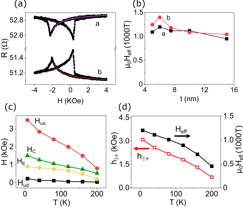
Figure 4(a) shows the same data as in Fig. 2(b), but now fitted using Eqs. (17), (18), with the power-law exponent for Py(7.5) determined from the micromagnetic simulations described above. Both this fitting and the fitting with in Fig. 2(b) provide good fits for the data. This shows that, in contrast to the micromagnetic simulations, the power-law exponent cannot be accurately determined from the experimental data. The reason for this discrepancy is that the values and of resistance in the saturated states with the magnetization perpendicular and parallel to current, respectively, as well as the parallel component of the effective exchange field, cannot be independently determined, and must be thus treated as additional fitting parameters. The experimental data do not provide sufficient information to accurately determine these parameters together with .
While fitting the experimental vs curves does not allow us to determine , we can still establish whether the observed behaviors are consistent with the uncorrelated random field approximation. We use the approach similar to that described in Section III, where we have shown that the correlated effective field approximation cannot describe the magnetization state for the field aligned with the cooling field [see Fig. 2(d)]. We fit the curves for different thicknesses of Py with Eqs. (17), (18), using the thickness-dependent values of and obtained from the micromagnetic simulations. Each such fitting independently yields the value of the effective exchange field . The uncrorrelated random field approximation is valid if the obtained values of are independent of . However, if the effective exchange field is correlated, then the values of extracted from such fitting should increase with , because in contrast to the uncorrelated field, the effects of the correlated field are not averaged out by larger thickness.
Figure 4(b) shows the values of determined from the fits of for different Py thicknesses. The values exhibit modest variations around the average value of T, and appear to slightly decrease at large , but clearly do not increase, as would be expected for the correlated field. We note that our procedure for calculating the values of involves multiple sources of random and systematic errors, including the uncertainty of the thicknesses of Py, slight variations of the deposition conditions resulting in the variation of among different samples, as well as the uncertainty of the fitting itself. These uncertainties are difficult to estimate a priori, warranting more detailed studies of multiple similar samples to assess them statistically. Nevertheless, the results shown in Fig. 4(b) for five samples with different thicknesses provide strong evidence for the validity of random-field approximation. Furthermore, the magnitude of of about T is about 10 times smaller than the typical strength of the nearest-neighbor exchange interactions in magnetic materials O’Handley 2000, as would be expected given that the spin-flop of AF spins at the F/AF interface results in their partial alignment Koon 1997; Schulthess and Butler 1998.
Our approach to quantifying the effective exchange fields in F/AF bilayers is validated by the analysis of the relationship between these fields and the essential characteristics of the magnetic hysteresis loop, the coercivity and the exchange bias field . Here, () is the magnetization reversal field on the down (up) sweep, signified by the sharp peaks in vs curves [see Fig. 4(b)]. The exchange bias field is generally attributed to the unidirectional anisotropy, while the enhanced coercivity is attributed to the uniaxial anisotropy acquired by F due to the exchange interaction at the F/AF interface.
Our approach allowed us to determine the value of , the net effective exchange field experienced by Py, separately for the magnetization orientation parallel to the cooling field [by fitting branches a,b with Eqs. (17), (18)], and for the magnetization orientation opposite to the cooling field [by fitting branches c,d with Eqs. (6), (7)]. We label the corresponding two values and . The effective unidirectional and uniaxial anisotropy fields can be then directly determined as and , respectively. We emphasize that these values are determined by fitting the curves for small deviations from saturation at large fields, completely independently from , that characterize magnetization reversal at small fields.
Figure 4(c) shows the temperature dependences of all four characteristics , , , and , for the Py(6)/CoO(6) sample at K. At higher temperatures, the deviations from saturation were too small to reliably determine by fitting the curve. The relations among , , , and are consistent with the results for a similar Py/CoO bilayer system, obtained by a completely different technique of transverse ac susceptibility Urazhdin et al. 2019. In particular, that study showed that the unidirectional anisotropy in this system is much smaller than the effective exchange bias field, and does not follow the temperature dependence of the latter. The data in Fig. 4(c) are consistent with this observation. Transverse ac susceptibility measurements also showed that and are about half of , and approximately follow the temperature dependence of the latter. These observations are also confirmed by the results in Fig. 4(c). While these results may seem surprising, they are consistent with the analysis of Ref. Urazhdin et al. 2019, which suggested that the asymmetry of the hysteresis loop for the Py/CoO bilayers is predominantly caused not by the unidirectional anisotropy, but rather by the different mechanisms of magnetization reversal between the two opposite magnetization states stabilized by the uniaxial anisotropy. We discuss the underlying mechanism in Section VII.
The random field , determined by fitting branches and of the curve with Eqs. (17) and (18), decreases with increasing temperature [solid symbols and right scale in Fig. 4(d)], following the same overall trends as [open symbols and left scale in Fig. 4(d)]. The similarity between the behaviors of these two quantities is a manifestation of their common origin from the exchange interaction at the Py/CoO interface.
VII Summary and conclusions
To summarize our findings, we have developed a new method for studying random effective exchange fields at magnetic interfaces, which extends the previously developed approaches to analyzing the effects of bulk random effective fields on 2d and 3d systems Chudnovsky 1983; Tejada et al. 1991; Garanin et al. 2013. Our method utilizes measurements of deviations from saturation characterized by - the average of the square of the angle between the magnetization and the external field - which follows a power-law dependence on the applied field with the exponent dependent on the characteristics of the exchange field. For the random effective exchange field correlated on the length scales exceeding the magnetic correlation length, the exponent is different from that for the uncorrelated random field, allowing one to distinguish between these two limiting cases. Moreover, the power-law exponent varies as a function of the film thickness, due to the correlations associated with averaging of the effective random field through the magnetic film thickness. By extension, we expect that the specific value of the power-law exponent for a given film thickness, if known precisely, can be utilized to determine the correlation length of random field. We leave analysis of this possibility to future studies.
We have employed our method to study effective exchange fields at the interfaces of Permalloy/CoO bilayers, a classic ferromagnet/antiferromagnet (F/AF) bilayer system extensively studied in the context of exchange bias. We utilizied magnetoelectronic measurements, in which resistance variations provide direct information about deviations from the saturated magnetization state. Analysis of our measurements required that several additional unknown parameters are determined from the data fitting, which did not allow us to directly determine the power-law exponent characterizing the correlations of random effective exchange field. Nevertheless, using the fact that the strength of the interaction at the interface must be independent of the film thickness, we showed that the results for the applied field parallel to the cooling field cannot be explained in terms of a correlated random effective field, but are consistent with the uncorrelated field approximation. In contrast, the results for the magnetic field direction antiparallel to the cooling field were in a reasonable agreement with the correlated effective exchange field approximation.
Qualitatively, we attribute the surprising difference between the characteristics for the two opposite field directions to the exchange-spring effects in CoO, which may produce quasi-uniform exchange torques over length scales comparable to the grain sizes of polycrystalline CoO. We also note that our surprising observations are consistent with a recent observation, for similar Permalloy/CoO bilayers, of qualitatively different reversal mechanisms between the two opposite directions of Py magnetization Urazhdin et al. 2019. Specifically, transverse ac susceptibility measurements showed that magnetization reversal from the magnetization direction opposite to the field-cooling direction into the direction aligned with the latter, occurs as soon as its energy becomes higher. Because of the large magnetic anisotropy barrier, such reversal must occur via inhomogeneus intermediate magnetization states, for example by domain wall motion.
On the other hand, reversal from the field-cooling direction was shown to occur only when the anisotropy barrier was almost compensated by the external field, indicating that the domain wall propagation is suppressed in this state, and reversal proceeds via quasi-uniform rotation. Our results complement this picture, providing additional clues about the underlying mechanisms. Indeed, uncorrelated random effective field is expected to result in efficient domain wall pinning, suppressing domain wall propagation. On the other hand, correlated random field, inferred from the analysis for the reversed magnetization state and attributed to the formation of AF exchange spring, may be expected to facilitate reversal through inhomogeneous magnetization state, consistent with the prior observations.
We now discuss the broader impact of our results on the studies and applications of thin magnetic film systems. First, the effective exchange field in F/AF bilayers, which is the focus of our study, is just one specific case of many magnetic interfacial effects extensively researched and commonly utilized in the existing and emerging technologies. Those include the Ruderman–Kittel–Kasuya–Yosida (RKKY) interaction commonly employed in magnetic multilayer sensors and in artificial antiferromagnets, interfacial magnetic anisotropies commonly utilized to induce perpendicular magnetic anisotropy in magnetic heterostructures, and the interfacial Dzyaloshinski-Moriya interaction Heck 2013; Chappert et al. 2010; O’Handley 2000. Understanding the spatial characteristics of these effects is crucial for the development of efficient and reproducible nanodevices. We note that the magnetic anisotropy is equivalent to effective fields for small-angle variations of magnetization, and therefore can be analyzed using the same approach as introduced above.
Our method becomes particularly effective if the saturation magnetization of the studied magnetic films is known, and if measurements of deviations from saturation utilize magnetometry, instead of the less direct magnetic characterization by magnetoelectronic techniques used in our study. For almost saturated states, magnetometry provides the value of , which allows one to directly extract , without any additional fitting parameters that were required in our magnetoelectronic measurements. This makes it possible to determine the power-law exponent characterizing the magnetic hysteresis curves, and thus the correlation length of the effective exchange fields, for a single magnetic heterostructure with a specific thickness of the magnetic layer.
Finally, we mention some of the projected fundamental insights that can become facilitated by our work. Our demonstration of uncorrelated effective random field effects in F/AF heterostructures opens the possibility to explore important fundamental consequences of these effects, such as topologically nontrivial magnetization states Proctor et al. 2014; Garanin et al. 2013. Such states can profoundly affect the magnetic properties, but to the best of our knowledge, their effects in F/AF heterostructures have not yet been explored. Another potentially profound consequence of magnetic frustration associated with uncorrelated effective random fields is the possibility to engineer magnetic energy landscapes whose energy scale is determined by the exchange interaction, rather than the magnetic anisotropy as in unfrustrated magnetic systems. The former is three to four orders of magnitude larger than the latter, providing a unique opportunity to develop ultrasmall thermally stable nanomagnetic devices.
The contributions to this work by G.C. and D.C. were supported by the NSF grant No. ECCS-1804198, the contribution by S.U. was supported by the U.S. Department of Energy (DOE), Basic Energy Sciences (BES), under Award # DE-SC0018976.
References
- Meiklejohn and Bean (1957) W. H. Meiklejohn and C. P. Bean, Phys. Rev. 105, 904 (1957).
- Heck (2013) C. Heck, Magnetic materials and their applications (Elsevier, 2013).
- Åkerman (2005) J. Åkerman, Science 308, 508 (2005), https://science.sciencemag.org/content/308/5721/508.full.pdf .
- Hu et al. (2011) J.-M. Hu, Z. Li, L.-Q. Chen, and C.-W. Nan, Nature communications 2, 553 (2011).
- Chappert et al. (2010) C. Chappert, A. Fert, and F. N. Van Dau, in Nanoscience And Technology: A Collection of Reviews from Nature Journals (World Scientific, 2010) pp. 147–157.
- Jungwirth et al. (2016) T. Jungwirth, X. Marti, P. Wadley, and J. Wunderlich, Nature Nanotechnology 11, 231 (2016).
- Sinova and Žutić (2012) J. Sinova and I. Žutić, Nature materials. 11, 368 (2012).
- Nishitani et al. (2010) J. Nishitani, K. Kozuki, T. Nagashima, and M. Hangyo, Applied Physics Letters 96, 221906 (2010).
- Ghosh and Manchon (2017) S. Ghosh and A. Manchon, Phys. Rev. B 95, 035422 (2017).
- Scholl et al. (2004) A. Scholl, M. Liberati, E. Arenholz, H. Ohldag, and J. Stöhr, Phys. Rev. Lett. 92, 247201 (2004).
- Reichlová et al. (2015) H. Reichlová, D. Kriegner, V. Holý, K. Olejník, V. Novák, M. Yamada, K. Miura, S. Ogawa, H. Takahashi, T. Jungwirth, and J. Wunderlich, Phys. Rev. B 92, 165424 (2015).
- Zhang et al. (2014) W. Zhang, M. B. Jungfleisch, W. Jiang, J. E. Pearson, A. Hoffmann, F. Freimuth, and Y. Mokrousov, Phys. Rev. Lett. 113, 196602 (2014).
- Fukami et al. (2016) S. Fukami, C. Zhang, S. DuttaGupta, A. Kurenkov, and H. Ohno, Nature Materials 15, 535 (2016).
- Lin and Chien (2017) W. Lin and C. L. Chien, Phys. Rev. Lett. 118, 067202 (2017).
- Prakash et al. (2016) A. Prakash, J. Brangham, F. Yang, and J. P. Heremans, Phys. Rev. B 94, 014427 (2016).
- Khymyn et al. (2017) R. Khymyn, I. Lisenkov, V. Tiberkevich, B. A. Ivanov, and A. Slavin, Scientific Reports 7, 43705 (2017).
- Nogués and Schuller (1999) J. Nogués and I. K. Schuller, Journal of Magnetism and Magnetic Materials 192, 203 (1999).
- Mauri et al. (1987) D. Mauri, H. C. Siegmann, P. S. Bagus, and E. Kay, Journal of Applied Physics 62, 3047 (1987).
- Nowak et al. (2002) U. Nowak, K. D. Usadel, J. Keller, P. Miltényi, B. Beschoten, and G. Güntherodt, Phys. Rev. B 66, 014430 (2002).
- Schlenker et al. (1986) C. Schlenker, S. Parkin, J. Scott, and K. Howard, Journal of Magnetism and Magnetic Materials 54-57, 801 (1986).
- Yamada et al. (2007) T. K. Yamada, E. Martínez, A. Vega, R. Robles, D. Stoeffler, A. L. V. de Parga, T. Mizoguchi, and H. van Kempen, Nanotechnology 18, 235702 (2007).
- Ding et al. (2013) J. Ding, O. Lebedev, S. Turner, Y. Tian, W. Hu, J. Seo, C. Panagopoulos, W. Prellier, G. Van Tendeloo, and T. Wu, Physical Review B 87, 054428 (2013).
- Malozemoff (1987) A. Malozemoff, Physical review B 35, 3679 (1987).
- Imry and Ma (1975) Y. Imry and S.-k. Ma, Phys. Rev. Lett. 35, 1399 (1975).
- Malozemoff (1988) A. P. Malozemoff, Phys. Rev. B 37, 7673 (1988).
- Araújo et al. (2002) A. E. P. d. Araújo, F. L. A. Machado, A. R. Rodrigues, A. Azevedo, F. M. de Aguiar, J. R. L. de Almeida, S. M. Rezende, and W. F. Egelhoff, Journal of Applied Physics 91, 7754 (2002).
- Jiménez et al. (2009) E. Jiménez, J. Camarero, J. Sort, J. Nogués, N. Mikuszeit, J. M. García-Martín, A. Hoffmann, B. Dieny, and R. Miranda, Physical Review B 80, 014415 (2009).
- Urazhdin and Danilenko (2015) S. Urazhdin and U. Danilenko, Physical Review B 92, 174416 (2015).
- Ma et al. (2016) T. Ma, X. Cheng, S. Boettcher, S. Urazhdin, and L. Novozhilova, Phys. Rev. B 94, 024422 (2016).
- Ma and Urazhdin (2018) T. Ma and S. Urazhdin, Phys. Rev. B 97, 054402 (2018).
- Urazhdin et al. (2019) S. Urazhdin, W. Li, and L. Novozhilova, Journal of Magnetism and Magnetic Materials 476, 75 (2019).
- Chudnovsky (1983) E. M. Chudnovsky, Journal of Magnetism and Magnetic Materials 40, 21 (1983).
- Garanin et al. (2013) D. A. Garanin, E. M. Chudnovsky, and T. Proctor, Phys. Rev. B 88, 224418 (2013).
- Proctor et al. (2014) T. C. Proctor, D. A. Garanin, and E. M. Chudnovsky, Phys. Rev. Lett. 112, 097201 (2014).
- Garanin and Chudnovsky (2015) D. A. Garanin and E. M. Chudnovsky, The European Physical Journal B 88, 81 (2015).
- Tejada et al. (1991) J. Tejada, B. Martinez, A. Labarta, and E. M. Chudnovsky, Physical Review B 44, 7698 (1991).
- Koon (1997) N. C. Koon, Phys. Rev. Lett. 78, 4865 (1997).
- Schulthess and Butler (1998) T. C. Schulthess and W. H. Butler, Phys. Rev. Lett. 81, 4516 (1998).
- Stiles and McMichael (1999) M. D. Stiles and R. D. McMichael, Phys. Rev. B 59, 3722 (1999).
- Urazhdin et al. (2008) S. Urazhdin, P. Tabor, and W.-L. Lim, Phys. Rev. B 78, 052403 (2008).
- Vansteenkiste et al. (2014) A. Vansteenkiste, J. Leliaert, M. Dvornik, M. Helsen, F. Garcia-Sanchez, and B. Van Waeyenberge, AIP advances 4, 107133 (2014).
- O’Handley (2000) R. C. O’Handley, Modern magnetic materials:principles and applications (Wiley, New York, 2000).