跳到论文正文
W Papers独立论文阅读器 arXiv:2003.06218 论文正文 计算阅读时间 · 0%
引用这篇论文根据当前论文元数据生成,正式投稿前建议核对。


License: arXiv.org perpetual non-exclusive license
arXiv:2003.06218v1 [q-fin.CP] 13 Mar 2020

Asymptotic expansion for the transition densities of stochastic differential equations driven by the gamma processes

Fan Jiang Thanks: School of Mathematical Sciences, Peking University, China, Email: jiangfmath@pku.edu.cn    Xin Zang Thanks: Corresponding author. School of Mathematical Sciences, Peking University, China, Email: xzang@pku.edu.cn    Jingping Yang Thanks: School of Mathematical Sciences, Peking University, China, Email: yangjp@math.pku.edu.cn
August 11, 2026
Abstract

In this paper, enlightened by the asymptotic expansion methodology developed by Li 2013b and Li and Chen 2016, we propose a Taylor-type approximation for the transition densities of the stochastic differential equations (SDEs) driven by the gamma processes, a special type of Lévy processes. After representing the transition density as a conditional expectation of Dirac delta function acting on the solution of the related SDE, the key technical method for calculating the expectation of multiple stochastic integrals conditional on the gamma process is presented. To numerically test the efficiency of our method, we examine the pure jump Ornstein–Uhlenbeck (OU) model and its extensions to two jump-diffusion models. For each model, the maximum relative error between our approximated transition density and the benchmark density obtained by the inverse Fourier transform of the characteristic function is sufficiently small, which shows the efficiency of our approximated method.

1 Introduction

It is known that Lévy-driven stochastic differential equations (SDEs) have been discussed in detail (Applebaum 2009; Kunita 2019; Kohatsu-Higa and Takeuchi 2019). The jump-diffusion SDE driven by the gamma process, as one important type of the Lévy-driven SDEs, has been widely used in finance. For instance, the Ornstein–Uhlenbeck (OU) type SDEs driven by the gamma processes were applied for modeling the short rate (Eberlein et al. 2013) and the returns of S&P 500 index (James et al. 2017). The various sensitivity indices for the asset price dynamics driven by the gamma processes were discussed in Kawai and Takeuchi 2010 and Kawai and Takeuchi 2011. Note that the gamma process is a pure-jump increasing Lévy process (Yor 2007; Cont and Tankov 2004; Applebaum 2009). Starting from the gamma process, the variance gamma process was defined (Madan and Seneta 1990; Madan et al. 1998).

For the financial applications mentioned above, the transition densities of the related SDEs play a vital role (Barndorff-Nielsen et al. 2001; Schoutens 2003). However, except for some special cases, the transition densities or even characteristic functions of the SDEs usually do not admit closed-form formulas, which brings difficulties for related applications. In this paper, enlightened by the asymptotic expansion method presented in Li 2013b and Li and Chen 2016, we propose a Taylor-type closed-form expansion for the transition density of the jump-diffusion SDE driven by the gamma process.

For the jump-diffusion SDE driven by the gamma process, we start from representing its transition density as a conditional expectation of a Dirac delta function acting on the solution of the related SDE, by applying the theory of Malliavin calculus (Kanwal 2004; Hayashi 2008; Ishikawa 2013; Kunita 2019). The main challenge in our method is to calculate the expectation of the product of the values of a gamma process at different intermediate times, conditional on the value of this gamma process at the terminal time. Consequently, through the distributional property of gamma bridge discussed in Ribeiro and Webber 2004, we express this type of conditional expectation as a polynomial function of the value of this gamma process at the terminal time. In this context, the expansion term of the transition density for any finite order can be analytically calculated in an efficient manner.

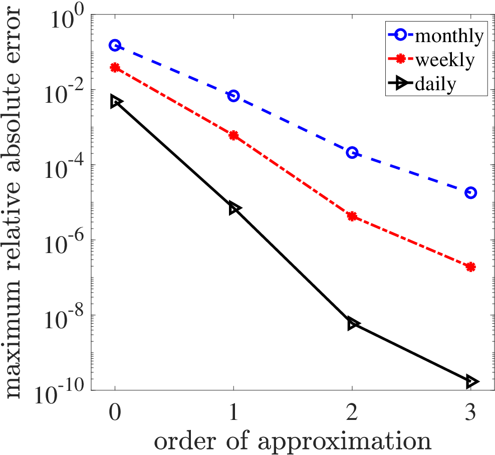
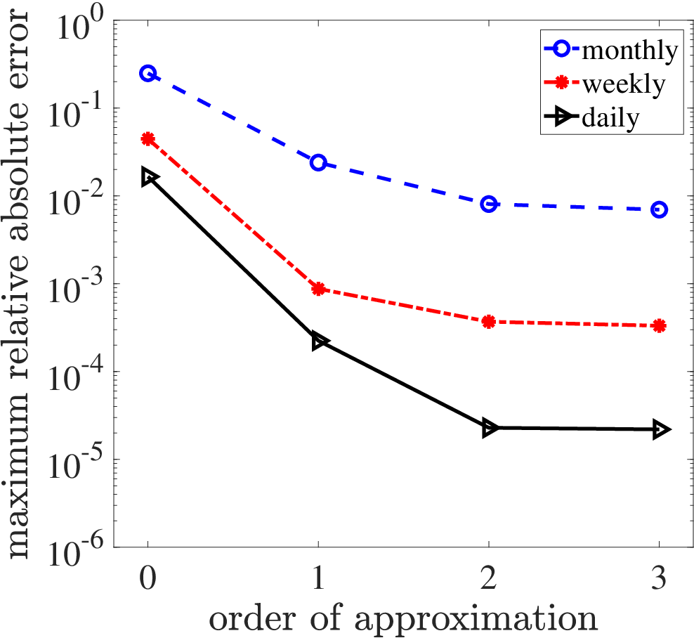
To illustrate the efficiency of our method, we conduct numerical analyses through three examples of the SDEs driven by the gamma processes, i.e., the pure jump OU model, along with its extensions to the constant diffusion and the square-root diffusion models. For each model, we compare the true transition density obtained by the inverse Fourier transform of its characteristic function with the approximated density obtained by our proposed asymptotic expansion method. The numerical results show that our approximated transition density can be efficiently calculated and converge rapidly to the true density.

The rest of this paper is organized as follows. Section 2 lays our model setup and gives the general expression of the asymptotic expansion. Section 3 provides detailed procedures for explicitly representing the expansion terms. Section 4 exhibits the numerical performance of our expansion method through three concrete examples. Section 5 concludes the paper.

2 The model setup and approximation methodology

2.1 Preliminaries of Dirac delta function

Before introducing our asymptotic expansion methodology, we first give a brief introduction of the Dirac delta function. Please refer to Kanwal 2004, Hayashi 2008, Ishikawa 2013 and Kunita 2019 for more details.

For ease of exposition later, we introduce the following notations and concepts. Denote by 𝒮′​(ℝ)\mathcal{S}^{\prime}(\mathbb{R}) the set of all real-valued tempered distributions. According to Section 6.2 in Kanwal 2004, the Dirac delta function denoted as δ⁡(⋅)\delta\left(\cdot\right) and its associated derivative operators dℓ​δ​(⋅)d​xℓ\frac{d^{\ell}\delta\left(\cdot\right)}{dx^{\ell}}\ for ℓ≥1\ell\geq 1 belong to 𝒮′​(ℝ)\mathcal{S}^{\prime}(\mathbb{R}). Here, for each ℓ≥1\ell\geq 1, the derivative operator dℓ​δ​(⋅)d​xℓ\frac{d^{\ell}\delta\left(\cdot\right)}{dx^{\ell}} is defined through an inner product with an indefinitely differentiable function f⁡(⋅)f(\cdot) with compact support on ℝ\mathbb{R}, i.e.,

⟨dℓ​δ​(x−y)d​xℓ,f⁡(x)⟩x=(−1)ℓ​⟨δ⁡(x−y),dℓ​fd​xℓ​(x)⟩x\left\langle\frac{d^{\ell}\delta(x-y)}{dx^{\ell}},f(x)\right\rangle_{x}=(-1)^{\ell}\left\langle\delta(x-y),\frac{d^{\ell}f}{dx^{\ell}}(x)\right\rangle_{x} (1)

for a fixed y∈ℝy\in\mathbb{R}, where the inner product ⟨f⁡(x),g⁡(x)⟩x:=∫−∞∞f⁡(x)​g​(x)​𝑑x\left\langle f\left(x\right),g\left(x\right)\right\rangle_{x}:=\int_{\mathbb{-\infty}}^{\infty}f(x)g(x)dx, see Section 2.6 in Kanwal 2004 for more details.

Let D∞​(ℝ)D_{\infty}(\mathbb{R}) be the set of all real-valued smooth Wiener-Poisson functionals and D∞′​(ℝ)D_{\infty}^{\prime}(\mathbb{R}) be the set of all real-valued generalized Wiener-Poisson functionals (Kunita 2019). According to Theorem 5.12.1 and equation (5.175) in Kunita 2019, for a tempered distribution Φ∈𝒮′​(ℝ)\Phi\in\mathcal{S}^{\prime}(\mathbb{R}), a regular nondegenerate Wiener-Poisson functional F∈D∞​(ℝ)F\in D_{\infty}(\mathbb{R}) and a smooth Wiener-Poisson functional G∈D∞​(ℝ)G\in D_{\infty}(\mathbb{R}), the generalized expectation 𝔼⁡[⋅]\mathbb{E}\left[\cdot\right] is defined as

𝔼⁡[Φ⁡(F)⋅G]:=12​π​∫−∞+∞∫−∞+∞e−i​v​x​Φ​(x)​E​[G​ei​v​F]​𝑑x​𝑑v,\mathbb{E}\left[\Phi\left(F\right)\cdot G\right]:=\frac{1}{2\pi}\int_{-\infty}^{+\infty}\int_{\mathbb{-\infty}}^{+\infty}e^{-ivx}\Phi\left(x\right)E\left[Ge^{ivF}\right]dxdv, (2)

where FF and GG can be treated as the random variables on the Wiener-Poisson space and the expectation in the right-hand side of (2) is the usual expectation in common sense. Hereafter, the notations 𝔼⁡[⋅]\mathbb{E}\left[\cdot\right] and E⁡[⋅]E\left[\cdot\right] represent the generalized expectation and usual expectation respectively.

For a fixed y∈ℝy\in\mathbb{R}, when we take Φ(⋅)=δ(⋅−y)\Phi(\cdot)=\delta(\cdot-y) and G≡1G\equiv 1 in (2), from the equation

∫−∞+∞e−i​v​x​δ​(x−y)​𝑑x=e−i​v​y,\int_{\mathbb{-\infty}}^{+\infty}e^{-ivx}\delta(x-y)dx=e^{-ivy}, (3)

we obtain that

𝔼⁡[δ⁡(F−y)]=12​π​∫−∞∞e−i​v​y​E​[ei​v​F]​𝑑v.\mathbb{E}\left[\delta\left(F-y\right)\right]=\frac{1}{2\pi}\int_{\mathbb{-\infty}}^{\infty}e^{-ivy}E\left[e^{ivF}\right]dv. (4)

Moreover, the regular nondegenerate Wiener-Poisson functional FF in (4) can also be taken as the strong solution of a homogeneous jump-diffusion SDE satisfying the nondegenerate bounded (NDB) condition, see Sections 3.5 – 3.6 in Ishikawa 2013 for more details. Especially, taking F≡0F\equiv 0 in (4), we can obtain that

δ⁡(y)=12​π​∫−∞+∞ei​v​y​𝑑v.\delta\left(y\right)=\frac{1}{2\pi}\int_{-\infty}^{+\infty}e^{ivy}dv. (5)

Given a parameter ϵ>0\epsilon>0, let F⁡(ϵ)F(\epsilon) be a regular Wiener-Poisson functional in D∞​(ℝ)D_{\infty}(\mathbb{R}). For example, F⁡(ϵ)F\left(\epsilon\right) can be taken as the strong solution of some jump-diffusion SDE with a parameter ϵ>0\epsilon>0. In the remaining of this section, for a fixed y∈ℝy\in\mathbb{R}, we introduce some theoretical results about the asymptotic expansion of δ⁡(F⁡(ϵ)−y)\delta(F(\epsilon)-y) with respect to the parameter ϵ\epsilon (see Section 4.1 of Ishikawa 2013). We assume that the functional F⁡(ϵ)F(\epsilon) satisfies the uniformly nondegenerate condition (Definition 4.1 in Ishikawa 2013), and has an expansion

F⁡(ϵ)=∑j=0∞fj​ϵjF\left(\epsilon\right)=\sum_{j=0}^{\infty}f_{j}\epsilon^{j} (6)

with respect to the norm in D∞​(ℝ)D_{\infty}(\mathbb{R}), where f0,f1,f2,…f_{0},f_{1},f_{2},\ldots are smooth Wiener-Poisson functionals.

According to Theorem 4.1 of Ishikawa 2013, for each fixed y∈ℝy\in\mathbb{R}, δ⁡(F⁡(ϵ)−y)\delta\left(F\left(\epsilon\right)-y\right) belongs to D∞′​(ℝ)D_{\infty}^{\prime}(\mathbb{R}) and has an asymptotic expansion

δ⁡(F⁡(ϵ)−y)=∑m=0MΦm​(y)​ϵm+𝒪⁡(ϵM+1)\delta\left(F\left(\epsilon\right)-y\right)=\sum_{m=0}^{M}\Phi_{m}(y)\epsilon^{m}+\mathcal{O}(\epsilon^{M+1}) (7)

with respect to the norm in D∞′​(ℝ)D_{\infty}^{\prime}(\mathbb{R}), where M∈ℕM\in\mathbb{N} denotes an arbitrary order of the expansion. Given the functionals {f0,f1,f2,…}\left\{f_{0},f_{1},f_{2},\ldots\right\} defined by (6), the coefficients Φm​(y)∈D∞′​(ℝ)\Phi_{m}(y)\in D_{\infty}^{\prime}(\mathbb{R}) for m≥0m\geq 0 can be expressed as

Φ0​(y)=δ⁡(f0−y)​ and ​Φm​(y)=∑(ℓ,(j1,j2,⋯,jℓ))∈𝒮m1ℓ!​dℓ​δ​(f0−y)d​xℓ​∏i=1ℓfji​ for ​m≥1,\Phi_{0}(y)=\delta\left(f_{0}-y\right)\text{ and }\Phi_{m}(y)=\sum_{\left(\ell,\left(j_{1},j_{2},\cdots,j_{\ell}\right)\right)\in\mathcal{S}_{m}}\frac{1}{\ell!}\frac{d^{\ell}\delta\left(f_{0}-y\right)}{dx^{\ell}}\prod\limits_{i=1}^{\ell}f_{j_{i}}\text{ for }m\geq 1, (8)

where the index set 𝒮m\mathcal{S}_{m} is defined as

𝒮m\displaystyle\mathcal{S}_{m} :={(ℓ,𝐣(ℓ))|ℓ=1,2,…, 𝐣(ℓ)=(j1,j2,…,jℓ) with j1,j2,…,jℓ≥1\displaystyle:=\left\{\left.\left(\ell,\mathbf{j}\left(\ell\right)\right)\right|\ell=1,2,\ldots,\text{ }\mathbf{j}\left(\ell\right)=\left(j_{1},j_{2},\ldots,j_{\ell}\right)\text{ with }j_{1},j_{2},\ldots,j_{\ell}\geq 1\right.
and j1+j2+⋯+jℓ=m}.\displaystyle\text{ \ \ \ \ }\left.\text{and }j_{1}+j_{2}+\cdots+j_{\ell}=m\right\}. (9)

For example, the coefficients Φ1​(y)\Phi_{1}(y) and Φ2​(y)\Phi_{2}(y) are given by

Φ1​(y)=f1​d​δ​(f0−y)d​x​ and ​Φ2​(y)=f2​d​δ​(f0−y)d​x+12​f12​d2​δ​(f0−y)d​x2.\Phi_{1}(y)=f_{1}\frac{d\delta\left(f_{0}-y\right)}{dx}\text{ and }\Phi_{2}(y)=f_{2}\frac{d\delta\left(f_{0}-y\right)}{dx}+\frac{1}{2}f_{1}^{2}\frac{d^{2}\delta\left(f_{0}-y\right)}{dx^{2}}.

According to Section 4 in Ishikawa 2013, by taking the generalized expectation defined in (2) on both sides of equation (7), we can obtain that

𝔼⁡[δ⁡(F⁡(ϵ)−y)]=∑m=0M𝔼⁡[Φm​(y)]​ϵm+𝒪⁡(ϵM+1).\mathbb{E}\left[\delta\left(F\left(\epsilon\right)-y\right)\right]=\sum_{m=0}^{M}\mathbb{E}\left[\Phi_{m}(y)\right]\epsilon^{m}+\mathcal{O}(\epsilon^{M+1}). (10)

For example, the terms 𝔼​[Φ0​(y)]\mathbb{E}\left[\Phi_{0}(y)\right] and 𝔼​[Φ1​(y)]\mathbb{E}\left[\Phi_{1}(y)\right] in (10) can be evaluated via (1), (2) and (3) as

𝔼⁡[Φ0​(y)]=𝔼⁡[δ⁡(f0−y)]=12​π​∫−∞+∞e−i​v​y​E​[ei​v​f0]​𝑑v\mathbb{E}\left[\Phi_{0}(y)\right]=\mathbb{E}[\delta\left(f_{0}-y\right)]=\frac{1}{2\pi}\int_{-\infty}^{+\infty}e^{-ivy}E[e^{ivf_{0}}]dv

and

𝔼⁡[Φ1​(y)]=𝔼⁡[f1​d​δ​(f0−y)d​x]=12​π​∫−∞+∞i​v​e−i​v​y​E​[f1​ei​v​f0]​𝑑v.\mathbb{E}\left[\Phi_{1}(y)\right]=\mathbb{E}[f_{1}\frac{d\delta\left(f_{0}-y\right)}{dx}]=\frac{1}{2\pi}\int_{-\infty}^{+\infty}ive^{-ivy}E[f_{1}e^{ivf_{0}}]dv.

In the subsequent calculation of the expansion terms for the transition density, by using equation (2), we will transform some specific generalized expectations like 𝔼​[Φm​(y)]\mathbb{E}\left[\Phi_{m}(y)\right] into the usual expectations.

2.2 The model setup

In this paper, we consider the following homogeneous jump-diffusion SDE driven by a gamma process

dX(t)=μ(X(t);𝜽)dt+σ(X(t);𝜽)dW(t)+dL(t), X(0)=x0,dX(t)=\mu(X(t);\bm{\theta})dt+\sigma(X(t);\bm{\theta})dW(t)+dL(t),\text{ }X\left(0\right)=x_{0}, (11)

where the functions μ⁡(x,𝜽)\mu\left(x;\bm{\theta}\right) and σ⁡(x,𝜽)\sigma(x;\bm{\theta}) are assumed to depend on some parameter vector 𝜽\bm{\theta} belonging to an open bound set Θ\Theta, {W⁡(t),t≥0}\left\{W(t),t\geq 0\right\} is a Brownian motion and {L⁡(t),t≥0}\left\{L(t),t\geq 0\right\} is a gamma process. Moreover, we assume that the gamma process {L⁡(t),t≥0}\left\{L(t),t\geq 0\right\} starts at L⁡(0)=0L(0)=0 with the density function

pL⁡(t)(x)=ba​t​xa​t−1​e−b​xΓ⁡(a​t), x≥0p_{L\left(t\right)}\left(x\right)=\frac{b^{at}x^{at-1}e^{-bx}}{\Gamma\left(at\right)},\text{ }x\geq 0 (12)

at time t>0t>0, where aa and bb are positive constants, and Γ⁡(⋅)\Gamma(\cdot) denotes the gamma function. The two processes {W⁡(t),t≥0}\left\{W(t),t\geq 0\right\} and {L⁡(t),t≥0}\left\{L(t),t\geq 0\right\} are independent. The characteristic function of the gamma process L⁡(t)L(t) is calculated as

E​ei​λ​L​(t)=(1−i​λb)−a​t≜exp⁡[t​ψL​(λ)],Ee^{i\lambda L(t)}=\left(1-\frac{i\lambda}{b}\right)^{-at}\triangleq\exp\left[t\psi_{L}\left(\lambda\right)\right], (13)

where ψL​(λ)=−a​log⁡(1−i​λ/b)\psi_{L}\left(\lambda\right)=-a\log\left(1-i\lambda/b\right) is the characteristic exponent of L⁡(t)L(t).

To guarantee the existence and uniqueness of the strong solution X⁡(t)X(t) of SDE (11) and obtain other desirable properties for implementing our method, the following standard and technical assumptions are assumed in this paper:

Assumption 1.

The diffusion function σ⁡(x,𝛉)\sigma\left(x;\bm{\theta}\right) satisfies that infx∈ℝσ⁡(x,𝛉)>0\inf_{x\in\mathbb{R}}\sigma\left(x;\bm{\theta}\right)>0 for any 𝛉∈Θ\bm{\theta}\in\Theta.

Assumption 2.

For each k∈ℕ+k\in\mathbb{N}_{+}, the kk-th order partial derivatives in xx of μ⁡(x,𝛉)\mu\left(x;\bm{\theta}\right) and σ⁡(x,𝛉)\sigma(x;\bm{\theta}) are uniformly bounded for any (x,𝛉)∈ℝ×Θ\left(x,\bm{\theta}\right)\in\mathbb{R}\times\Theta.

Assumption 3.

The functions μ⁡(x,𝛉)\mu\left(x;\bm{\theta}\right) and σ⁡(x,𝛉)\sigma(x;\bm{\theta}) satisfy the linear growth conditions

|μ⁡(x,𝜽)|≤c1​(1+|x|)​ and ​|σ⁡(x,𝜽)|≤c2​(1+|x|),\left|\mu\left(x;\bm{\theta}\right)\right|\leq c_{1}\left(1+\left|x\right|\right)\text{ and }\left|\sigma\left(x;\bm{\theta}\right)\right|\leq c_{2}\left(1+\left|x\right|\right),

for some c1,c2∈ℝ+c_{1},c_{2}\in\mathbb{R}_{+} and any (x,𝛉)∈ℝ×Θ\left(x,\bm{\theta}\right)\in\mathbb{R}\times\Theta.

Assumption 1 and Assumption 2 guarantee the NDB condition and uniformly nondegenerate condition for justifying the validity and convergence of our proposed asymptotic expansion method, which will be shown in section 2.3. Assumption 2 and Assumption 3 guarantee the existence and uniqueness of the strong solution X⁡(t)X(t) of SDE (11).

2.3 The expansion of the transition density

For the jump-diffusion SDE (11), by the time-homogeneity nature, the transition density of X⁡(t+Δ)X\left(t+\Delta\right) given X⁡(t)=x0X\left(t\right)=x_{0} can be expressed as

ℙ(X(t+Δ)∈dx|X(t)=x0;𝜽)=pX⁡(Δ)(x|x0;𝜽)dx,\mathbb{P}\left(\left.X\left(t+\Delta\right)\in dx\right|X\left(t\right)=x_{0};\bm{\theta}\right)=p_{X\left(\Delta\right)}\left(x|x_{0};\bm{\theta}\right)dx, (14)

where Δ\Delta denotes the time interval. For most SDEs defined in (11), their transition densities do not admit closed-form expressions. Even for some special cases with closed-form conditional characteristic functions, the inversion to transition densities may not be easy, especially for the pure jump processes (Barndorff-Nielsen et al. 2001; Schoutens 2003). In the following, we propose a closed-form expansion for approximating the transition density pX⁡(Δ)​(x|x0;𝜽)p_{X\left(\Delta\right)}\left(x|x_{0};\bm{\theta}\right) of the jump-diffusion SDE (11).

To start with, we parameterize the dynamics of X⁡(t)X(t) in (11) via a parameter ϵ∈(0,1]\epsilon\in\left(0,1\right] as

dX(ϵ,t)=ϵ[μ(X(ϵ,t);𝜽)dt+σ(X(ϵ,t);𝜽)dW(t)+dL(t)], X(ϵ,0)=x0.dX(\epsilon,t)=\epsilon\left[\mu(X(\epsilon,t);\bm{\theta})dt+\sigma\left(X(\epsilon,t);\bm{\theta}\right)dW(t)+dL(t)\right],\text{ }X(\epsilon,0)=x_{0}. (15)

Note that the solution X⁡(ϵ,t)X(\epsilon,t) of (15) satisfies X⁡(ϵ,t)|ϵ=1=X⁡(t)\left.X(\epsilon,t)\right|_{\epsilon=1}=X(t). By regarding ϵ∈(0,1]\epsilon\in\left(0,1\right] as an extra element of the parameter vector, we see that the SDE (15) still satisfies Assumption 2 and Assumption 3, which implies the existence and uniqueness of the strong solution X⁡(ϵ,t)X(\epsilon,t) (Platen and Bruti-Liberati 2010). The transition density of X⁡(ϵ,t)X(\epsilon,t) in (15) can be expressed as

ℙ(X(ϵ,t+Δ)∈dx|X(ϵ,t)=x0;𝜽)=pX⁡(ϵ,Δ)(x|x0;𝜽)dx.\mathbb{P}\left(\left.X(\epsilon,t+\Delta)\in dx\right|X\left(\epsilon,t\right)=x_{0};\bm{\theta}\right)=p_{X\left(\epsilon,\Delta\right)}\left(x|x_{0};\bm{\theta}\right)dx. (16)

Once we obtain an asymptotic expansion of pX⁡(ϵ,Δ)​(x|x0;𝜽)p_{X\left(\epsilon,\Delta\right)}\left(x|x_{0};\bm{\theta}\right) as a series of ϵ\epsilon, the transition density pX⁡(Δ)(x|x0;𝜽)p_{X\left(\Delta\right)}\left(\left.x\right|x_{0};\bm{\theta}\right) in (14) can be obtained by letting ϵ=1\epsilon=1.

To derive the asymptotic expansion of pX⁡(ϵ,Δ)​(x|x0;𝜽)p_{X\left(\epsilon,\Delta\right)}\left(x|x_{0};\bm{\theta}\right) in (16), we first claim that X⁡(ϵ,t)X(\epsilon,t) satisfies the NDB condition introduced in Section 2.1, which will justify the representation of the transition density pX⁡(ϵ,Δ)​(x|x0;𝜽)p_{X\left(\epsilon,\Delta\right)}\left(x|x_{0};\bm{\theta}\right) as a conditional expectation shown below. Note that for X⁡(ϵ,t)X(\epsilon,t), the NDB condition introduced from Definition 3.5 in Ishikawa 2013 is transformed to the condition that σ⁡(x,𝜽)≠0\sigma\left(x;\bm{\theta}\right)\neq 0 for any (x,𝜽)∈ℝ×Θ\left(x,\bm{\theta}\right)\in\mathbb{R}\times\Theta, which is guaranteed by Assumption 1.

Based on the NDB condition and the time-homogeneity nature of X⁡(ϵ,t)X(\epsilon,t), we represent
pX⁡(ϵ,Δ)​(x|x0;𝜽)p_{X\left(\epsilon,\Delta\right)}\left(x|x_{0};\bm{\theta}\right) as a conditional expectation of Dirac delta function acting on X⁡(ϵ,Δ)−xX\left(\epsilon,\Delta\right)-x by

pX⁡(ϵ,Δ)(x|x0;𝜽)=𝔼[δ(X(ϵ,Δ)−x)|X(ϵ,0)=x0;𝜽].p_{X\left(\epsilon,\Delta\right)}\left(\left.x\right|x_{0};\bm{\theta}\right)=\mathbb{E}\left[\left.\delta\left(X\left(\epsilon,\Delta\right)-x\right)\right|X(\epsilon,0)=x_{0};\bm{\theta}\right]. (17)

The validity of (17) will be verified in Remark 1 below in detail. For brevity, we omit the initial condition X⁡(ϵ,0)=x0X(\epsilon,0)=x_{0} and drop the dependence of 𝜽\bm{\theta} in the dynamics of (11) and (15) hereafter, unless especially noted. The starting point of the expansion for (17) lies in that X⁡(ϵ,Δ)X\left(\epsilon,\Delta\right) admits the pathwise Taylor-type expansion

X⁡(ϵ,Δ)=∑m=0MXm​(Δ)​ϵm+𝒪⁡(ϵM+1),X\left(\epsilon,\Delta\right)=\sum_{m=0}^{M}X_{m}(\Delta)\epsilon^{m}+\mathcal{O}(\epsilon^{M+1}), (18)

where M∈ℕM\in\mathbb{N} denotes an arbitrary order of expansion, see, e.g., Chapter 4 in Platen and Bruti-Liberati 2010 for the validity of this expansion.

In the following, we first derive the expressions of the expansion terms Xm​(Δ)X_{m}(\Delta) in (18). We rewrite (15) in integrated form as

X⁡(ϵ,Δ)=x0+ϵ⁡[∫0Δμ⁡(X⁡(ϵ,s))​𝑑s+∫0Δσ⁡(X⁡(ϵ,s))​𝑑W​(s)+L⁡(Δ)].X(\epsilon,\Delta)=x_{0}+\epsilon\left[\int_{0}^{\Delta}\mu(X(\epsilon,s))ds+\int_{0}^{\Delta}\sigma\left(X(\epsilon,s)\right)dW(s)+L(\Delta)\right]. (19)

Letting ϵ↓0\epsilon\downarrow 0 on both sides in (19), we have

X⁡(0,Δ)=x0X(0,\Delta)=x_{0} (20)

for any fixed Δ≥0\Delta\geq 0. Further, from the expansion of X⁡(ϵ,Δ)X\left(\epsilon,\Delta\right) in (18), we can obtain that

μ⁡(X⁡(ϵ,t)):=∑m=0Mμm​(t)​ϵm+𝒪⁡(ϵM+1)\mu\left(X(\epsilon,t)\right):=\sum_{m=0}^{M}\mu_{m}(t)\epsilon^{m}+\mathcal{O}(\epsilon^{M+1}) (21)

and

σ⁡(X⁡(ϵ,t)):=∑m=0Mσm​(t)​ϵm+𝒪⁡(ϵM+1)\sigma\left(X(\epsilon,t)\right):=\sum_{m=0}^{M}\sigma_{m}(t)\epsilon^{m}+\mathcal{O}(\epsilon^{M+1}) (22)

in the SDE (15), where

μm​(t):=1m!​dm​μ​(X⁡(ϵ,t))d​ϵm|ϵ=0=∑(ℓ,(j1,j2,⋯,jℓ))∈𝒮m1ℓ!​dℓ​μ​(x0)d​xℓ​∏i=1ℓXji​(t)\mu_{m}(t):=\frac{1}{m!}\left.\frac{d^{m}\mu\left(X(\epsilon,t)\right)}{d\epsilon^{m}}\right|_{\epsilon=0}=\sum_{\left(\ell,\left(j_{1},j_{2},\cdots,j_{\ell}\right)\right)\in\mathcal{S}_{m}}\frac{1}{\ell!}\frac{d^{\ell}\mu\left(x_{0}\right)}{dx^{\ell}}\prod\limits_{i=1}^{\ell}X_{j_{i}}\left(t\right) (23)

and

σm​(t):=1m!​dm​σ​(X⁡(ϵ,t))d​ϵm|ϵ=0=∑(ℓ,(j1,j2,⋯,jℓ))∈𝒮m1ℓ!​dℓ​σ​(x0)d​xℓ​∏i=1ℓXji​(t)\sigma_{m}(t):=\frac{1}{m!}\left.\frac{d^{m}\sigma\left(X(\epsilon,t)\right)}{d\epsilon^{m}}\right|_{\epsilon=0}=\sum_{\left(\ell,\left(j_{1},j_{2},\cdots,j_{\ell}\right)\right)\in\mathcal{S}_{m}}\frac{1}{\ell!}\frac{d^{\ell}\sigma\left(x_{0}\right)}{dx^{\ell}}\prod\limits_{i=1}^{\ell}X_{j_{i}}\left(t\right) (24)

with the index set 𝒮m\mathcal{S}_{m} defined by (9) and the condition X⁡(0,t)=x0X(0,t)=x_{0} as in (20). Plugging (18), (21), and (22) into (19), we have

∑m=0MXm​(Δ)​ϵm+𝒪⁡(ϵM+1)\displaystyle\sum_{m=0}^{M}X_{m}(\Delta)\epsilon^{m}+\mathcal{O}(\epsilon^{M+1})
=\displaystyle= x0+∑m=0M(∫0Δμm​(s)​𝑑s+∫0Δσm​(s)​𝑑W​(s))​ϵm+1+ϵ​L​(Δ)+𝒪⁡(ϵM+2).\displaystyle x_{0}+\sum_{m=0}^{M}\left(\int_{0}^{\Delta}\mu_{m}(s)ds+\int_{0}^{\Delta}\sigma_{m}(s)dW(s)\right)\epsilon^{m+1}+\epsilon L(\Delta)+\mathcal{O}(\epsilon^{M+2}).

By comparing the coefficients of ϵm\epsilon^{m} for m=0,1,2,…m=0,1,2,\ldots, we conclude that X0​(Δ)≡x0X_{0}\left(\Delta\right)\equiv x_{0},

X1​(Δ)=μ⁡(x0)​Δ+σ⁡(x0)​W​(Δ)+L⁡(Δ),X_{1}\left(\Delta\right)=\mu\left(x_{0}\right)\Delta+\sigma(x_{0})W(\Delta)+L\left(\Delta\right), (25)

and

Xm​(Δ)=∫0Δμm−1​(s)​𝑑s+∫0Δσm−1​(s)​𝑑W​(s)​ for ​m≥2,X_{m}(\Delta)=\int_{0}^{\Delta}\mu_{m-1}(s)ds+\int_{0}^{\Delta}\sigma_{m-1}(s)dW(s)\text{ for }m\geq 2, (26)

where μm−1​(s)\mu_{m-1}(s) and σm−1​(s)\sigma_{m-1}(s) are defined in equations (23) and (24) respectively. As the expressions μm−1​(s)\mu_{m-1}(s) and σm−1​(s)\sigma_{m-1}(s) involved in the right-hand side of (26) are determined by the expansion terms X0​(s),X_{0}\left(s\right), X1​(s),…,Xm−1​(s)X_{1}(s),\ldots,X_{m-1}(s) in (18) with orders at most m−1m-1, we notice that Xm​(Δ)X_{m}(\Delta) is fully determined by Xi​(s),i=0,1,2,…,m−1X_{i}(s),i=0,1,2,\ldots,m-1 for all 0≤s≤Δ0\leq s\leq\Delta.

Next, we illustrate the expansion of pX⁡(ϵ,Δ)​(x|x0;𝜽)p_{X\left(\epsilon,\Delta\right)}\left(x|x_{0};\bm{\theta}\right) in (17) as a convergent series of ϵ\epsilon. To do this, we standardize X⁡(ϵ,Δ)X(\epsilon,\Delta) into

Y⁡(ϵ,Δ)=X⁡(ϵ,Δ)−x0σ⁡(x0)​Δ​ϵ,Y(\epsilon,\Delta)=\frac{X(\epsilon,\Delta)-x_{0}}{\sigma(x_{0})\sqrt{\Delta}\epsilon}, (27)

from which the transition density pX⁡(ϵ,Δ)​(x|x0;𝜽)p_{X\left(\epsilon,\Delta\right)}\left(x|x_{0};\bm{\theta}\right) in (17) can be represented in terms of Y⁡(ϵ,Δ)Y\left(\epsilon,\Delta\right) as

pX⁡(ϵ,Δ)​(x|x0;𝜽)=1σ⁡(x0)​Δ​ϵ​𝔼​[δ⁡(Y⁡(ϵ,Δ)−y)]|y=x−x0σ⁡(x0)​Δ​ϵ.p_{X\left(\epsilon,\Delta\right)}\left(x|x_{0};\bm{\theta}\right)=\left.\frac{1}{\sigma(x_{0})\sqrt{\Delta}\epsilon}\mathbb{E}\left[\delta\left(Y\left(\epsilon,\Delta\right)-y\right)\right]\right|_{y=\frac{x-x_{0}}{\sigma(x_{0})\sqrt{\Delta}\epsilon}}. (28)

According to Hayashi and Ishikawa 2012 and Definition 4.1 in Ishikawa 2013, Y⁡(ϵ,Δ)Y(\epsilon,\Delta) in (27) satisfies the uniformly nondegenerate condition which is guaranteed by Assumption 1 and Assumption 2. Then the expectation in the right-hand side of (28) admits a convergent series of ϵ\epsilon. To obtain an expansion of 𝔼⁡[δ⁡(Y⁡(ϵ,Δ)−y)]\mathbb{E}\left[\delta\left(Y\left(\epsilon,\Delta\right)-y\right)\right] in (28) with respect to ϵ\epsilon, we notice from (18), (27) and X0​(Δ)≡x0X_{0}\left(\Delta\right)\equiv x_{0} that

Y⁡(ϵ,Δ)=∑m=0MYm​(Δ)​ϵm+𝒪⁡(ϵM+1),Y\left(\epsilon,\Delta\right)=\sum_{m=0}^{M}Y_{m}(\Delta)\epsilon^{m}+\mathcal{O}(\epsilon^{M+1}), (29)

where

Ym(Δ)=Xm+1​(Δ)σ⁡(x0)​Δ, for m=0,1,2,….Y_{m}(\Delta)=\frac{X_{m+1}(\Delta)}{\sigma(x_{0})\sqrt{\Delta}},\text{ for }m=0,1,2,\ldots. (30)

Since the functional δ(⋅−y)\delta\left(\cdot-y\right) belongs to 𝒮′​(ℝ)\mathcal{S}^{\prime}(\mathbb{R}), according to (7), we obtain a Taylor-type expansion of δ⁡(Y⁡(ϵ,Δ)−y)\delta\left(Y\left(\epsilon,\Delta\right)-y\right) as

δ⁡(Y⁡(ϵ,Δ)−y)=∑m=0MΦm​(y)​ϵm+𝒪⁡(ϵM+1)\delta\left(Y\left(\epsilon,\Delta\right)-y\right)=\sum_{m=0}^{M}\Phi_{m}(y)\epsilon^{m}+\mathcal{O}(\epsilon^{M+1}) (31)

for any M∈ℕM\in\mathbb{N}. Here in (31), it follows from (8), (29) and (30) that

Φ0​(y)=δ⁡(Y0​(Δ)−y)\Phi_{0}\left(y\right)=\delta\left(Y_{0}(\Delta)-y\right) (32)

and

Φm​(y)=∑(ℓ,(j1,j2,⋯,jℓ))∈𝒮m1ℓ!​1(σ⁡(x0)​Δ)ℓ​dℓ​δ​(Y0​(Δ)−y)d​xℓ​∏i=1ℓXji+1​(Δ)\Phi_{m}(y)=\sum_{\left(\ell,\left(j_{1},j_{2},\cdots,j_{\ell}\right)\right)\in\mathcal{S}_{m}}\frac{1}{\ell!}\frac{1}{(\sigma(x_{0})\sqrt{\Delta})^{\ell}}\frac{d^{\ell}\delta\left(Y_{0}(\Delta)-y\right)}{dx^{\ell}}\prod\limits_{i=1}^{\ell}X_{j_{i}+1}(\Delta) (33)

for m≥1m\geq 1, with the index set 𝒮m\mathcal{S}_{m} defined in (9) and Y0​(Δ)=X1​(Δ)σ⁡(x0)​ΔY_{0}(\Delta)=\frac{X_{1}(\Delta)}{\sigma(x_{0})\sqrt{\Delta}}. Further, based on (10), we take the generalized expectation on both sides of (31) to obtain that

𝔼⁡[δ⁡(Y⁡(ϵ,Δ)−y)]=∑m=0MΩm​(y)​ϵm+𝒪⁡(ϵM+1),\mathbb{E}\left[\delta\left(Y\left(\epsilon,\Delta\right)-y\right)\right]=\sum_{m=0}^{M}\Omega_{m}(y)\epsilon^{m}+\mathcal{O}(\epsilon^{M+1}), (34)

where the generalized expectation Ωm​(y):=𝔼​Φm​(y)\Omega_{m}\left(y\right):=\mathbb{E}\Phi_{m}\left(y\right) for m≥0m\geq 0 will be explicitly derived and transformed into some usual expectation below.

For simplicity, we name Ω0​(y)\Omega_{0}\left(y\right) and Ωm​(y)\Omega_{m}\left(y\right) for m≥1m\geq 1 in (34) the leading term and the higher-order terms respectively. Combining (28) and (34) by letting ϵ=1\epsilon=1, the approximated transition density of X⁡(Δ)X(\Delta) up to the MM-th order is proposed as

pX⁡(Δ)(M)(x|x0;𝜽):=1σ⁡(x0)​Δ∑m=0MΩm(x−x0σ⁡(x0)​Δ).p_{X\left(\Delta\right)}^{\left(M\right)}\left(\left.x\right|x_{0};\bm{\theta}\right):=\frac{1}{\sigma(x_{0})\sqrt{\Delta}}\sum_{m=0}^{M}\Omega_{m}\left(\frac{x-x_{0}}{\sigma(x_{0})\sqrt{\Delta}}\right). (35)

Consequently, to approximate the transition density pX⁡(Δ)(x|x0;𝜽)p_{X\left(\Delta\right)}\left(\left.x\right|x_{0};\bm{\theta}\right) in (14) up to any finite order, it suffices to specify the functions Ω0​(y)\Omega_{0}\left(y\right) and Ωm​(y)\Omega_{m}\left(y\right) for m≥1m\geq 1 in (35), which will be investigated in Section 2.4.

Remark 1.

The equation (17) can be verified as follows. According to Section 6.4 in Kunita 2019, under the initial condition X⁡(ϵ,0)=x0X\left(\epsilon,0\right)=x_{0}, the strong solution X⁡(ϵ,t)X\left(\epsilon,t\right) of SDE (15) is uniquely tied to a stochastic flow, which is a regular Wiener-Poisson functional belonging to the set D∞​(ℝ)D_{\infty}(\mathbb{R}) (Section 3.1 in Kunita 2019). Thus, by noting that X⁡(ϵ,t)X(\epsilon,t) satisfies the NDB condition, under the initial condition X⁡(ϵ,0)=x0X\left(\epsilon,0\right)=x_{0}, we take F=X⁡(ϵ,Δ)F=X\left(\epsilon,\Delta\right) in (4) to obtain that

𝔼[δ(X(ϵ,Δ)−x)|X(ϵ,0)=x0;𝜽]\displaystyle\mathbb{E}\left[\left.\delta\left(X\left(\epsilon,\Delta\right)-x\right)\right|X(\epsilon,0)=x_{0};\bm{\theta}\right]
=\displaystyle= 12​π∫−∞+∞e−i​v​xE[ei​v​X​(ϵ,Δ)|X(ϵ,0)=x0;𝜽]dv=pX⁡(ϵ,Δ)(x|x0;𝜽),\displaystyle\frac{1}{2\pi}\int_{-\infty}^{+\infty}e^{-ivx}E\left[\left.e^{ivX\left(\epsilon,\Delta\right)}\right|X(\epsilon,0)=x_{0};\bm{\theta}\right]dv=p_{X\left(\epsilon,\Delta\right)}\left(x|x_{0};\bm{\theta}\right),

which verifies (17).

Remark 2.

The above closed-form expansion method can also be applied to the special case of SDE (11) with σ⁡(X⁡(t),𝜽)≡0\sigma(X(t);\bm{\theta})\equiv 0. In this context, we only adjust the above algorithm to standardize X⁡(ϵ,Δ)X\left(\epsilon,\Delta\right) defined by (15) into

Y⁡(ϵ,Δ)=X⁡(ϵ,Δ)−x0ϵY\left(\epsilon,\Delta\right)=\frac{X\left(\epsilon,\Delta\right)-x_{0}}{\epsilon}

instead of (27), which implies that

𝔼⁡[δ⁡(X⁡(ϵ,Δ)−x)]=1ϵ​𝔼​[δ⁡(Y⁡(ϵ,Δ)−y)]|y=x−x0ϵ.\mathbb{E}\left[\delta\left(X\left(\epsilon,\Delta\right)-x\right)\right]=\left.\frac{1}{\epsilon}\mathbb{E}\left[\delta\left(Y\left(\epsilon,\Delta\right)-y\right)\right]\right|_{y=\frac{x-x_{0}}{\epsilon}}.

The remaining procedures are performed in a similar manner. Therefore, the approximated transition density of X⁡(Δ)X(\Delta) up to the MM-th order can be obtained by

pX⁡(Δ)(M)(x|x0;𝜽)=∑m=0MΩm(x−x0),p_{X\left(\Delta\right)}^{\left(M\right)}\left(\left.x\right|x_{0};\bm{\theta}\right)=\sum_{m=0}^{M}\Omega_{m}\left(x-x_{0}\right), (36)

where Ωm​(y)=E​Φm​(y)\Omega_{m}(y)=E\Phi_{m}\left(y\right) and the terms Φm​(y)\Phi_{m}\left(y\right) are calculated by

Φ0​(y)=δ⁡(Y0​(Δ)−y)\Phi_{0}\left(y\right)=\delta\left(Y_{0}(\Delta)-y\right)

and

Φm​(y)=∑(ℓ,(j1,j2,⋯,jℓ))∈𝒮m1ℓ!​dℓ​δ​(Y0​(Δ)−y)d​xℓ​∏i=1ℓXji+1​(Δ)\Phi_{m}(y)=\sum_{\left(\ell,\left(j_{1},j_{2},\cdots,j_{\ell}\right)\right)\in\mathcal{S}_{m}}\frac{1}{\ell!}\frac{d^{\ell}\delta\left(Y_{0}(\Delta)-y\right)}{dx^{\ell}}\prod\limits_{i=1}^{\ell}X_{j_{i}+1}(\Delta)

for m≥1m\geq 1, with the index set 𝒮m\mathcal{S}_{m} defined in (9) and Y0​(Δ)=X1​(Δ)Y_{0}(\Delta)=X_{1}(\Delta).

2.4 General expressions of the leading term and high-order terms

In this part, we give the explicit expression of the leading term Ω0​(y)\Omega_{0}\left(y\right) and the general representations of the higher-order terms Ωm​(y)\Omega_{m}\left(y\right) for m≥1m\geq 1 defined in (34). Throughout this section, we denote by ϕ⁡(⋅)\phi\left(\cdot\right) the density function of a standard normal variable and recall that pL⁡(t)​(⋅)p_{L\left(t\right)}\left(\cdot\right) is the density function of the gamma process L⁡(t)L(t) given by (12).

From (32), the leading term Ω0​(y)\Omega_{0}\left(y\right) is expressed as

Ω0​(y)=𝔼⁡[δ⁡(Y0​(Δ)−y)],\Omega_{0}(y)=\mathbb{E}\left[\delta\left(Y_{0}(\Delta)-y\right)\right], (37)

which is exactly the density function of Y0​(Δ)Y_{0}(\Delta) evaluated at yy. The explicit expression of Ω0​(y)\Omega_{0}(y) is given in the following proposition.

Proposition 1.

The leading term Ω0​(y)\Omega_{0}\left(y\right) in (35) admits the following explicit expression

Ω0​(y)=∫0+∞ϕ⁡(y−μ⁡(x0)​Δ+uσ⁡(x0)​Δ)​pL⁡(Δ)​(u)​𝑑u,\Omega_{0}(y)=\int_{0}^{+\infty}\phi\left(y-\frac{\mu\left(x_{0}\right)\Delta+u}{\sigma(x_{0})\sqrt{\Delta}}\right)p_{L\left(\Delta\right)}\left(u\right)du,

where pL⁡(Δ)​(⋅)p_{L\left(\Delta\right)}(\cdot) is the density function of the gamma process L⁡(Δ)L(\Delta) given by (12).

Proof.

From (4) and (37), we obtain that

Ω0​(y)\displaystyle\Omega_{0}(y) =𝔼⁡[δ⁡(Y0​(Δ)−y)]\displaystyle=\mathbb{E}\left[\delta\left(Y_{0}(\Delta)-y\right)\right]
=12​π​∫−∞+∞e−i​v​y​E​[ei​v​Y0​(Δ)]​𝑑v\displaystyle=\frac{1}{2\pi}\int_{-\infty}^{+\infty}e^{-ivy}E\left[e^{ivY_{0}\left(\Delta\right)}\right]dv
=E[12​π∫−∞+∞e−i​v​yE[ei​v​Y0​(Δ)|L(Δ)]dv].\displaystyle=E\left[\frac{1}{2\pi}\int_{-\infty}^{+\infty}e^{-ivy}E\left[\left.e^{ivY_{0}\left(\Delta\right)}\right|L\left(\Delta\right)\right]dv\right]. (38)

We notice from (25) and (30) that Y0​(Δ)Y_{0}(\Delta) in (38) can be represented as

Y0​(Δ)=X1​(Δ)σ⁡(x0)​Δ=W⁡(Δ)Δ+μ⁡(x0)​Δ+L⁡(Δ)σ⁡(x0)​Δ.Y_{0}(\Delta)=\frac{X_{1}(\Delta)}{\sigma(x_{0})\sqrt{\Delta}}=\frac{W(\Delta)}{\sqrt{\Delta}}+\frac{\mu\left(x_{0}\right)\Delta+L\left(\Delta\right)}{\sigma(x_{0})\sqrt{\Delta}}. (39)

Here, conditioned on the jump term L⁡(Δ)L\left(\Delta\right), the variable Y0​(Δ)Y_{0}(\Delta) in (39) follows a normal distribution. Therefore, the inner term of the expectation in the last equation of (38) can be calculated as

12​π∫−∞+∞e−i​v​yE[ei​v​Y0​(Δ)|L(Δ)]dv\displaystyle\frac{1}{2\pi}\int_{-\infty}^{+\infty}e^{-ivy}E\left[\left.e^{ivY_{0}\left(\Delta\right)}\right|L\left(\Delta\right)\right]dv
=\displaystyle= E[12​π∫−∞+∞e−i​v​yei​v​(W⁡(Δ)Δ+μ⁡(x0)​Δ+L⁡(Δ)σ⁡(x0)​Δ)dv|L(Δ)]\displaystyle E\left[\left.\frac{1}{2\pi}\int_{-\infty}^{+\infty}e^{-ivy}e^{iv\left(\frac{W(\Delta)}{\sqrt{\Delta}}+\frac{\mu\left(x_{0}\right)\Delta+L\left(\Delta\right)}{\sigma(x_{0})\sqrt{\Delta}}\right)}dv\right|L\left(\Delta\right)\right]
=\displaystyle= ∫−∞∞E[12​π∫−∞+∞e−i​v​yei​v​(x+μ⁡(x0)​Δ+L⁡(Δ)σ⁡(x0)​Δ)dv|L(Δ)]ϕ(x)dx\displaystyle\int_{-\infty}^{\infty}E\left[\left.\frac{1}{2\pi}\int_{-\infty}^{+\infty}e^{-ivy}e^{iv\left(x+\frac{\mu\left(x_{0}\right)\Delta+L\left(\Delta\right)}{\sigma(x_{0})\sqrt{\Delta}}\right)}dv\right|L\left(\Delta\right)\right]\phi\left(x\right)dx
=\displaystyle= E[∫−∞∞(12​π∫−∞+∞e−i​v​yei​v​(x+μ⁡(x0)​Δ+L⁡(Δ)σ⁡(x0)​Δ)dv)ϕ(x)dx|L(Δ)].\displaystyle E\left[\left.\int_{-\infty}^{\infty}\left(\frac{1}{2\pi}\int_{-\infty}^{+\infty}e^{-ivy}e^{iv\left(x+\frac{\mu\left(x_{0}\right)\Delta+L\left(\Delta\right)}{\sigma(x_{0})\sqrt{\Delta}}\right)}dv\right)\phi\left(x\right)dx\right|L\left(\Delta\right)\right]. (40)

By the relation (5), we obtain that

12​π​∫−∞+∞e−i​v​y​ei​v​(x+μ⁡(x0)​Δ+L⁡(Δ)σ⁡(x0)​Δ)​𝑑v=δ⁡(x+μ⁡(x0)​Δ+L⁡(Δ)σ⁡(x0)​Δ−y).\frac{1}{2\pi}\int_{-\infty}^{+\infty}e^{-ivy}e^{iv\left(x+\frac{\mu\left(x_{0}\right)\Delta+L\left(\Delta\right)}{\sigma(x_{0})\sqrt{\Delta}}\right)}dv=\delta\left(x+\frac{\mu\left(x_{0}\right)\Delta+L\left(\Delta\right)}{\sigma(x_{0})\sqrt{\Delta}}-y\right).

Then plugging the above equation into (40) by noting the definition of the Dirac delta function, we obtain that

12​π∫−∞+∞e−i​v​yE[ei​v​Y0​(Δ)|L(Δ)]dv\displaystyle\frac{1}{2\pi}\int_{-\infty}^{+\infty}e^{-ivy}E\left[\left.e^{ivY_{0}\left(\Delta\right)}\right|L\left(\Delta\right)\right]dv =E[∫−∞∞δ(x+μ⁡(x0)​Δ+L⁡(Δ)σ⁡(x0)​Δ−y)ϕ(x)dx|L(Δ)]\displaystyle=E\left[\left.\int_{-\infty}^{\infty}\delta\left(x+\frac{\mu\left(x_{0}\right)\Delta+L\left(\Delta\right)}{\sigma(x_{0})\sqrt{\Delta}}-y\right)\phi\left(x\right)dx\right|L\left(\Delta\right)\right]
=E[ϕ(y−μ⁡(x0)​Δ+L⁡(Δ)σ⁡(x0)​Δ)|L(Δ)].\displaystyle=E\left[\left.\phi\left(y-\frac{\mu\left(x_{0}\right)\Delta+L\left(\Delta\right)}{\sigma(x_{0})\sqrt{\Delta}}\right)\right|L\left(\Delta\right)\right]. (41)

Plugging (41) into (38), the leading term Ω0​(y)\Omega_{0}(y) can be finally calculated as

Ω0(y)=E[E[ϕ(y−μ⁡(x0)​Δ+L⁡(Δ)σ⁡(x0)​Δ)|L(Δ)]]=∫0+∞ϕ(y−μ⁡(x0)​Δ+uσ⁡(x0)​Δ)pL⁡(Δ)(u)du.\Omega_{0}(y)=E\left[E\left[\left.\phi\left(y-\frac{\mu\left(x_{0}\right)\Delta+L\left(\Delta\right)}{\sigma(x_{0})\sqrt{\Delta}}\right)\right|L\left(\Delta\right)\right]\right]=\int_{0}^{+\infty}\phi\left(y-\frac{\mu\left(x_{0}\right)\Delta+u}{\sigma(x_{0})\sqrt{\Delta}}\right)p_{L\left(\Delta\right)}\left(u\right)du.

∎

To calculate the higher-order terms Ωm​(y)\Omega_{m}\left(y\right) for m≥1m\geq 1, we introduce the following notations. For ℓ≥1\ell\geq 1 and 𝐣⁡(ℓ)=(j1,j2,…,jℓ)\mathbf{j}\left(\ell\right)=\left(j_{1},j_{2},\ldots,j_{\ell}\right) with ji≥1j_{i}\geq 1, we define

K(ℓ,𝐣⁡(ℓ))(z1,z2):=E(∏i=1ℓXji+1(Δ)|W(Δ),L(Δ))|W⁡(Δ)=z1​Δ,L⁡(Δ)=z2.K_{\left(\ell,\mathbf{j}\left(\ell\right)\right)}\left(z_{1},z_{2}\right):=\left.E\left(\left.\prod\limits_{i=1}^{\ell}X_{j_{i}+1}(\Delta)\right|W(\Delta),L\left(\Delta\right)\right)\right|_{W\left(\Delta\right)=z_{1}\sqrt{\Delta},L\left(\Delta\right)=z_{2}}. (42)

Meanwhile, for any bivariate differentiable function u⁡(x,y)u(x,y) defined on ℝ2\mathbb{R}^{2}, we introduce the following partial differential operators with respect to the first variable:

𝒟1(1)​(u⁡(x,y)):=∂u⁡(x,y)∂x−x​u​(x,y)​ and ​𝒟1(n)​(u⁡(x,y)):=𝒟1(1)​(𝒟1(n−1)​(u⁡(x,y)))​ for ​n≥2.\mathcal{D}_{1}^{(1)}\left(u(x,y)\right):=\frac{\partial u(x,y)}{\partial x}-xu(x,y)\text{ and }\mathcal{D}_{1}^{(n)}\left(u(x,y)\right):=\mathcal{D}_{1}^{(1)}\left(\mathcal{D}_{1}^{(n-1)}\left(u(x,y)\right)\right)\text{ for }n\geq 2. (43)

The representations of Ωm​(y)\Omega_{m}\left(y\right) for m≥1m\geq 1 are given in the following theorem.

Theorem 1.

For any integer m≥1m\geq 1, the high-order term Ωm​(y)\Omega_{m}\left(y\right) in (35) admits the following expression:

Ωm​(y)=∑(ℓ,(j1,j2,⋯,jℓ))∈𝒮m(−1)ℓℓ!​1(σ⁡(x0)​Δ)ℓ​∫0+∞𝒟1(ℓ)​(K(ℓ,𝐣⁡(ℓ))​(z1,z2))⋅ϕ⁡(z1)⋅pL⁡(Δ)​(z2)​d​z2,\Omega_{m}(y)=\sum_{\left(\ell,\left(j_{1},j_{2},\cdots,j_{\ell}\right)\right)\in\mathcal{S}_{m}}\frac{(-1)^{{}^{\ell}}}{\ell!}\frac{1}{(\sigma(x_{0})\sqrt{\Delta})^{\ell}}\int_{0}^{+\infty}\mathcal{D}_{1}^{(\ell)}\left(K_{\left(\ell,\mathbf{j}\left(\ell\right)\right)}\left(z_{1},z_{2}\right)\right)\cdot\phi(z_{1})\cdot p_{L\left(\Delta\right)}(z_{2})dz_{2}, (44)

where the index set 𝒮m\mathcal{S}_{m} is defined in (9), pL⁡(Δ)​(⋅)p_{L\left(\Delta\right)}(\cdot) is the density function of the gamma process L⁡(Δ)L(\Delta) given by (12) and

z1=y−μ⁡(x0)​Δ+z2σ⁡(x0)​Δ.z_{1}=y-\frac{\mu\left(x_{0}\right)\Delta+z_{2}}{\sigma(x_{0})\sqrt{\Delta}}. (45)
Proof.

We see from the definition of Φm​(y)\Phi_{m}(y) in (33) that

Ωm​(y)\displaystyle\Omega_{m}(y) =𝔼​Φm​(y)=∑(ℓ,(j1,j2,⋯,jℓ))∈𝒮m𝔼⁡[1ℓ!​1(σ⁡(x0)​Δ)ℓ​dℓ​δ​(Y0​(Δ)−y)d​xℓ​∏i=1ℓXji+1​(Δ)]\displaystyle=\mathbb{E}\Phi_{m}(y)=\sum_{\left(\ell,\left(j_{1},j_{2},\cdots,j_{\ell}\right)\right)\in\mathcal{S}_{m}}\mathbb{E}\left[\frac{1}{\ell!}\frac{1}{(\sigma(x_{0})\sqrt{\Delta})^{\ell}}\frac{d^{\ell}\delta\left(Y_{0}(\Delta)-y\right)}{dx^{\ell}}\prod\limits_{i=1}^{\ell}X_{j_{i}+1}(\Delta)\right]
=∑(ℓ,(j1,j2,⋯,jℓ))∈𝒮m1ℓ!​1(σ⁡(x0)​Δ)ℓ​𝔼​[dℓ​δ​(Y0​(Δ)−y)d​xℓ​∏i=1ℓXji+1​(Δ)].\displaystyle=\sum_{\left(\ell,\left(j_{1},j_{2},\cdots,j_{\ell}\right)\right)\in\mathcal{S}_{m}}\frac{1}{\ell!}\frac{1}{(\sigma(x_{0})\sqrt{\Delta})^{\ell}}\mathbb{E}\left[\frac{d^{\ell}\delta\left(Y_{0}(\Delta)-y\right)}{dx^{\ell}}\prod\limits_{i=1}^{\ell}X_{j_{i}+1}(\Delta)\right]. (46)

For the generalized expectation in the last line of (46), according to (2), we have

𝔼⁡[dℓ​δ​(Y0​(Δ)−y)d​xℓ​∏i=1ℓXji+1​(Δ)]\displaystyle\mathbb{E}\left[\frac{d^{\ell}\delta\left(Y_{0}(\Delta)-y\right)}{dx^{\ell}}\prod\limits_{i=1}^{\ell}X_{j_{i}+1}(\Delta)\right]
=\displaystyle= 12​π​∫−∞+∞∫−∞+∞e−i​v​x​dℓ​δ​(x−y)d​xℓ​E​[∏i=1ℓXji+1​(Δ)⋅ei​v​Y0​(Δ)]​𝑑x​𝑑v\displaystyle\frac{1}{2\pi}\int_{-\infty}^{+\infty}\int_{-\infty}^{+\infty}e^{-ivx}\frac{d^{\ell}\delta\left(x-y\right)}{dx^{\ell}}E\left[\prod\limits_{i=1}^{\ell}X_{j_{i}+1}(\Delta)\cdot e^{ivY_{0}(\Delta)}\right]dxdv
=\displaystyle= ∫−∞+∞(12​π​∫−∞+∞e−i​v​x​dℓ​δ​(x−y)d​xℓ​𝑑x)​E​[∏i=1ℓXji+1​(Δ)⋅ei​v​Y0​(Δ)]​𝑑v.\displaystyle\int_{-\infty}^{+\infty}\left(\frac{1}{2\pi}\int_{-\infty}^{+\infty}e^{-ivx}\frac{d^{\ell}\delta\left(x-y\right)}{dx^{\ell}}dx\right)E\left[\prod\limits_{i=1}^{\ell}X_{j_{i}+1}(\Delta)\cdot e^{ivY_{0}(\Delta)}\right]dv.

By the relations (1) and (3), the above equation is further calculated as

𝔼⁡[dℓ​δ​(Y0​(Δ)−y)d​xℓ​∏i=1ℓXji+1​(Δ)]\displaystyle\mathbb{E}\left[\frac{d^{\ell}\delta\left(Y_{0}(\Delta)-y\right)}{dx^{\ell}}\prod\limits_{i=1}^{\ell}X_{j_{i}+1}(\Delta)\right]
=\displaystyle= ∫−∞+∞(12​π​(−1)ℓ​∫−∞+∞δ⁡(x−y)​dℓ​e−i​v​xd​xℓ​𝑑x)​E​[∏i=1ℓXji+1​(Δ)⋅ei​v​Y0​(Δ)]​𝑑v\displaystyle\int_{-\infty}^{+\infty}\left(\frac{1}{2\pi}\left(-1\right)^{\ell}\int_{-\infty}^{+\infty}\delta\left(x-y\right)\frac{d^{\ell}e^{-ivx}}{dx^{\ell}}dx\right)E\left[\prod\limits_{i=1}^{\ell}X_{j_{i}+1}(\Delta)\cdot e^{ivY_{0}(\Delta)}\right]dv
=\displaystyle= ∫−∞+∞12​π​(i​v)ℓ​e−i​v​y⋅E⁡[∏i=1ℓXji+1​(Δ)⋅ei​v​Y0​(Δ)]​𝑑v.\displaystyle\int_{-\infty}^{+\infty}\frac{1}{2\pi}\left(iv\right)^{\ell}e^{-ivy}\cdot E\left[\prod\limits_{i=1}^{\ell}X_{j_{i}+1}(\Delta)\cdot e^{ivY_{0}(\Delta)}\right]dv. (47)

Then following the definition of Y0​(Δ)Y_{0}\left(\Delta\right) in (39) and using the independence between Brownian motion W⁡(t)W(t) and gamma process L⁡(t)L(t), the expectation in the last line of (47) is calculated as

E⁡[∏i=1ℓXji+1​(Δ)⋅ei​v​Y0​(Δ)]\displaystyle E\left[\prod\limits_{i=1}^{\ell}X_{j_{i}+1}(\Delta)\cdot e^{ivY_{0}(\Delta)}\right]
=\displaystyle= E⁡[∏i=1ℓXji+1​(Δ)⋅ei​v​(W⁡(Δ)Δ+μ⁡(x0)​Δ+L⁡(Δ)σ⁡(x0)​Δ)]\displaystyle E\left[\prod\limits_{i=1}^{\ell}X_{j_{i}+1}(\Delta)\cdot e^{iv\left(\frac{W(\Delta)}{\sqrt{\Delta}}+\frac{\mu\left(x_{0}\right)\Delta+L\left(\Delta\right)}{\sigma(x_{0})\sqrt{\Delta}}\right)}\right]
=\displaystyle= ∫0∞∫−∞∞E[∏i=1ℓXji+1(Δ)⋅ei​v​(z1+μ⁡(x0)​Δ+z2σ⁡(x0)​Δ)|W(Δ),L(Δ)]|W⁡(Δ)=z1​Δ,L⁡(Δ)=z2\displaystyle\int_{0}^{\infty}\int_{-\infty}^{\infty}E\left.\left[\left.\prod\limits_{i=1}^{\ell}X_{j_{i}+1}(\Delta)\cdot e^{iv\left(z_{1}+\frac{\mu\left(x_{0}\right)\Delta+z_{2}}{\sigma(x_{0})\sqrt{\Delta}}\right)}\right|W(\Delta),L\left(\Delta\right)\right]\right|_{W(\Delta)=z_{1}\sqrt{\Delta},L\left(\Delta\right)=z_{2}}
×ϕ⁡(z1)​pL⁡(Δ)​(z2)​d​z1​d​z2​.\displaystyle\times\phi(z_{1})p_{L\left(\Delta\right)}(z_{2})dz_{1}dz_{2}\text{.} (48)

By the definition of K(ℓ,𝐣⁡(ℓ))​(z1,z2)K_{\left(\ell,\mathbf{j}\left(\ell\right)\right)}\left(z_{1},z_{2}\right) in (42), the expectation (48) can be expressed as

E⁡[∏i=1ℓXji+1​(Δ)⋅ei​v​Y0​(Δ)]=∫0∞∫−∞∞ei​v​(z1+μ⁡(x0)​Δ+z2σ⁡(x0)​Δ)​K(ℓ,𝐣⁡(ℓ))​(z1,z2)​ϕ​(z1)​pL⁡(Δ)​(z2)​d​z1​d​z2.E\left[\prod\limits_{i=1}^{\ell}X_{j_{i}+1}(\Delta)\cdot e^{ivY_{0}(\Delta)}\right]=\int_{0}^{\infty}\int_{-\infty}^{\infty}e^{iv\left(z_{1}+\frac{\mu\left(x_{0}\right)\Delta+z_{2}}{\sigma(x_{0})\sqrt{\Delta}}\right)}K_{\left(\ell,\mathbf{j}\left(\ell\right)\right)}\left(z_{1},z_{2}\right)\phi(z_{1})p_{L\left(\Delta\right)}(z_{2})dz_{1}dz_{2}. (49)

Plugging (49) into (47), we obtain that

​𝔼​[dℓ​δ​(Y0​(Δ)−y)d​xℓ​∏i=1ℓXji+1​(Δ)]\displaystyle\text{\ }\mathbb{E}\left[\frac{d^{\ell}\delta\left(Y_{0}(\Delta)-y\right)}{dx^{\ell}}\prod\limits_{i=1}^{\ell}X_{j_{i}+1}(\Delta)\right]
=\displaystyle= ∫−∞+∞12​π​(i​v)ℓ​e−i​v​y​∫0∞∫−∞∞ei​v​(z1+μ⁡(x0)​Δ+z2σ⁡(x0)​Δ)​K(ℓ,𝐣⁡(ℓ))​(z1,z2)​ϕ​(z1)​pL⁡(Δ)​(z2)​d​z1​d​z2​𝑑v\displaystyle\int_{-\infty}^{+\infty}\frac{1}{2\pi}\left(iv\right)^{\ell}e^{-ivy}\int_{0}^{\infty}\int_{-\infty}^{\infty}e^{iv\left(z_{1}+\frac{\mu\left(x_{0}\right)\Delta+z_{2}}{\sigma(x_{0})\sqrt{\Delta}}\right)}K_{\left(\ell,\mathbf{j}\left(\ell\right)\right)}\left(z_{1},z_{2}\right)\phi(z_{1})p_{L\left(\Delta\right)}(z_{2})dz_{1}dz_{2}dv
=\displaystyle= ∫0+∞∫−∞∞12​π​e−i​v​y​pL⁡(Δ)​(z2)​(∫−∞∞∂ℓei​v​(z1+μ⁡(x0)​Δ+z2σ⁡(x0)​Δ)∂z1ℓ​K(ℓ,𝐣⁡(ℓ))​(z1,z2)​ϕ​(z1)​d​z1)​𝑑v​d​z2.\displaystyle\int_{0}^{+\infty}\int_{-\infty}^{\infty}\frac{1}{2\pi}e^{-ivy}p_{L\left(\Delta\right)}(z_{2})\left(\int_{-\infty}^{\infty}\frac{\partial^{\ell}e^{iv\left(z_{1}+\frac{\mu\left(x_{0}\right)\Delta+z_{2}}{\sigma(x_{0})\sqrt{\Delta}}\right)}}{\partial z_{1}^{\ell}}K_{\left(\ell,\mathbf{j}\left(\ell\right)\right)}\left(z_{1},z_{2}\right)\phi(z_{1})dz_{1}\right)dvdz_{2}. (50)

Using integration by parts, the last line of (50) can be further calculated as

∫0+∞∫−∞∞12​πe−i​v​ypL⁡(Δ)(z2)∫−∞∞(−1)ℓei​v​(z1+μ⁡(x0)​Δ+z2σ⁡(x0)​Δ)∂ℓ(K(ℓ,𝐣⁡(ℓ))(z1,z2)ϕ(z1))∂z1ℓdz1dvdz2\displaystyle\text{\ }\int_{0}^{+\infty}\int_{-\infty}^{\infty}\frac{1}{2\pi}e^{-ivy}p_{L\left(\Delta\right)}(z_{2})\int_{-\infty}^{\infty}(-1)^{{}^{\ell}}e^{iv\left(z_{1}+\frac{\mu\left(x_{0}\right)\Delta+z_{2}}{\sigma(x_{0})\sqrt{\Delta}}\right)}\frac{\partial^{{}^{\ell}}\left(K_{\left(\ell,\mathbf{j}\left(\ell\right)\right)}\left(z_{1},z_{2}\right)\phi(z_{1})\right)}{\partial z_{1}^{{}^{\ell}}}dz_{1}dvdz_{2}
=\displaystyle= ∫0+∞∫−∞∞(∫−∞∞12​π​e−i​v​y​ei​v​(z1+μ⁡(x0)​Δ+z2σ⁡(x0)​Δ)​𝑑v)\displaystyle\int_{0}^{+\infty}\int_{-\infty}^{\infty}\left(\int_{-\infty}^{\infty}\frac{1}{2\pi}e^{-ivy}e^{iv\left(z_{1}+\frac{\mu\left(x_{0}\right)\Delta+z_{2}}{\sigma(x_{0})\sqrt{\Delta}}\right)}dv\right)
×(−1)ℓ∂ℓ(K(ℓ,𝐣⁡(ℓ))(z1,z2)ϕ(z1))∂z1ℓpL⁡(Δ)(z2)dz1dz2.\displaystyle\times(-1)^{{}^{\ell}}\frac{\partial^{{}^{\ell}}\left(K_{\left(\ell,\mathbf{j}\left(\ell\right)\right)}\left(z_{1},z_{2}\right)\phi(z_{1})\right)}{\partial z_{1}^{{}^{\ell}}}p_{L\left(\Delta\right)}(z_{2})dz_{1}dz_{2}. (51)

By the relation (5), it follows that

12​π​∫−∞+∞e−i​v​y​ei​v​(z1+μ⁡(x0)​Δ+z2σ⁡(x0)​Δ)​𝑑v=12​π​∫−∞+∞ei​v​(z1+μ⁡(x0)​Δ+z2σ⁡(x0)​Δ−y)​𝑑v=δ⁡(z1+μ⁡(x0)​Δ+z2σ⁡(x0)​Δ−y),\frac{1}{2\pi}\int_{-\infty}^{+\infty}e^{-ivy}e^{iv\left(z_{1}+\frac{\mu\left(x_{0}\right)\Delta+z_{2}}{\sigma(x_{0})\sqrt{\Delta}}\right)}dv=\frac{1}{2\pi}\int_{-\infty}^{+\infty}e^{iv\left(z_{1}+\frac{\mu\left(x_{0}\right)\Delta+z_{2}}{\sigma(x_{0})\sqrt{\Delta}}-y\right)}dv=\delta\left(z_{1}+\frac{\mu\left(x_{0}\right)\Delta+z_{2}}{\sigma(x_{0})\sqrt{\Delta}}-y\right),

Plugging the above equation into (51), we obtain that

​𝔼​[dℓ​δ​(Y0​(Δ)−y)d​xℓ​∏i=1ℓXji+1​(Δ)]\displaystyle\text{\ }\mathbb{E}\left[\frac{d^{\ell}\delta\left(Y_{0}(\Delta)-y\right)}{dx^{\ell}}\prod\limits_{i=1}^{\ell}X_{j_{i}+1}(\Delta)\right]
=\displaystyle= ∫0+∞∫−∞∞δ(z1+μ⁡(x0)​Δ+z2σ⁡(x0)​Δ−y)(−1)ℓ∂ℓ(K(ℓ,𝐣⁡(ℓ))(z1,z2)ϕ(z1))∂z1ℓpL⁡(Δ)(z2)dz1dz2\displaystyle\int_{0}^{+\infty}\int_{-\infty}^{\infty}\delta\left(z_{1}+\frac{\mu\left(x_{0}\right)\Delta+z_{2}}{\sigma(x_{0})\sqrt{\Delta}}-y\right)(-1)^{{}^{\ell}}\frac{\partial^{{}^{\ell}}\left(K_{\left(\ell,\mathbf{j}\left(\ell\right)\right)}\left(z_{1},z_{2}\right)\phi(z_{1})\right)}{\partial z_{1}^{{}^{\ell}}}p_{L\left(\Delta\right)}(z_{2})dz_{1}dz_{2}
=\displaystyle= ∫0+∞(−1)ℓ∂ℓ(K(ℓ,𝐣⁡(ℓ))(z1,z2)ϕ(z1))∂z1ℓ|z1=y−μ⁡(x0)​Δ+z2σ⁡(x0)​Δ⋅pL⁡(Δ)(z2)dz2.\displaystyle\int_{0}^{+\infty}(-1)^{{}^{\ell}}\left.\frac{\partial^{{}^{\ell}}\left(K_{\left(\ell,\mathbf{j}\left(\ell\right)\right)}\left(z_{1},z_{2}\right)\phi(z_{1})\right)}{\partial z_{1}^{{}^{\ell}}}\right|_{z_{1}=y-\frac{\mu\left(x_{0}\right)\Delta+z_{2}}{\sigma(x_{0})\sqrt{\Delta}}}\cdot p_{L\left(\Delta\right)}(z_{2})dz_{2}. (52)

Thus, plugging (52) into (46), we obtain that

Ωm​(y)\displaystyle\Omega_{m}(y) =∑(ℓ,(j1,j2,⋯,jℓ))∈𝒮m(−1)ℓℓ!​1(σ⁡(x0)​Δ)ℓ\displaystyle=\sum_{\left(\ell,\left(j_{1},j_{2},\cdots,j_{\ell}\right)\right)\in\mathcal{S}_{m}}\frac{(-1)^{{}^{\ell}}}{\ell!}\frac{1}{(\sigma(x_{0})\sqrt{\Delta})^{\ell}}
×∫0+∞∂ℓ(K(ℓ,𝐣⁡(ℓ))(z1,z2)ϕ(z1))∂z1ℓ|z1=y−μ⁡(x0)​Δ+z2σ⁡(x0)​Δ​pL⁡(Δ)​(z2)​d​z2.\displaystyle\text{ \ \ \ \ \ \ \ \ \ \ \ \ \ }\times\int_{0}^{+\infty}\left.\frac{\partial^{{}^{\ell}}\left(K_{\left(\ell,\mathbf{j}\left(\ell\right)\right)}\left(z_{1},z_{2}\right)\phi(z_{1})\right)}{\partial z_{1}^{{}^{\ell}}}\right|_{z_{1}=y-\frac{\mu\left(x_{0}\right)\Delta+z_{2}}{\sigma(x_{0})\sqrt{\Delta}}}p_{L\left(\Delta\right)}(z_{2})dz_{2}. (53)

From the definition (43), for any bivariate differentiable function u⁡(z1,z2)u\left(z_{1},z_{2}\right), we have

∂∂z1​(u⁡(z1,z2)​ϕ​(z1))=(∂u⁡(z1,z2)∂z1−z1​u​(z1,z2))​ϕ​(z1)≡𝒟1(1)​(u⁡(z1,z2))⋅ϕ⁡(z1),\frac{\partial}{\partial z_{1}}\left(u(z_{1},z_{2})\phi(z_{1})\right)=\left(\frac{\partial u(z_{1},z_{2})}{\partial z_{1}}-z_{1}u(z_{1},z_{2})\right)\phi(z_{1})\equiv\mathcal{D}_{1}^{(1)}\left(u(z_{1},z_{2})\right)\cdot\phi(z_{1}),

and

∂ℓ∂z1ℓ​(u⁡(z1,z2)​ϕ​(z1))=𝒟1(ℓ)​(u⁡(z1,z2))⋅ϕ⁡(z1)\frac{\partial^{\ell}}{\partial z_{1}^{\ell}}\left(u(z_{1},z_{2})\phi(z_{1})\right)=\mathcal{D}_{1}^{(\ell)}\left(u(z_{1},z_{2})\right)\cdot\phi(z_{1})

for any ℓ≥1\ell\geq 1, from which we obtain that

∂ℓ(K(ℓ,𝐣⁡(ℓ))​(z1,z2)​ϕ​(z1))∂z1ℓ=𝒟1(ℓ)​(K(ℓ,𝐣⁡(ℓ))​(z1,z2))⋅ϕ⁡(z1).\frac{\partial^{\ell}\left(K_{\left(\ell,\mathbf{j}\left(\ell\right)\right)}\left(z_{1},z_{2}\right)\phi(z_{1})\right)}{\partial z_{1}^{\ell}}=\mathcal{D}_{1}^{(\ell)}\left(K_{\left(\ell,\mathbf{j}\left(\ell\right)\right)}\left(z_{1},z_{2}\right)\right)\cdot\phi(z_{1}). (54)

Plugging (54) into (53), we obtain the formula (44). ∎

According to (44) in Theorem 1, to calculate the high-order terms Ωm​(y)\Omega_{m}(y) for m≥1m\geq 1, it suffices to derive the bivariate function K(ℓ,𝐣⁡(ℓ))​(z1,z2)K_{(\ell,\mathbf{j(}\ell))}(z_{1},z_{2}) in (42), which will be shown in Section 3.

3 Explicit calculation of K(ℓ,𝐣⁡(ℓ))​(z1,z2)K_{\left(\ell,\mathbf{j}\left(\ell\right)\right)}\left(z_{1},z_{2}\right)

In this section, we explicitly derive the function K(ℓ,𝐣⁡(ℓ))​(z1,z2)K_{\left(\ell,\mathbf{j}\left(\ell\right)\right)}\left(z_{1},z_{2}\right) for every fixed ℓ≥1\ell\geq 1 and 𝐣⁡(ℓ)=(j1,j2,…,jℓ)\mathbf{j}\left(\ell\right)=\left(j_{1},j_{2},\ldots,j_{\ell}\right) with ji≥1j_{i}\geq 1 in (42), from which we can evaluate Ωm​(y)\Omega_{m}\left(y\right) for m≥1m\geq 1 in (44) and obtain the approximated transition density pX⁡(Δ)(M)(x|x0;𝜽)p_{X\left(\Delta\right)}^{\left(M\right)}\left(\left.x\right|x_{0};\bm{\theta}\right) in (35). Moreover, for illustration purpose, the pure jump OU model, constant diffusion model and square-root diffusion model are introduced as examples of SDE (11) to exhibit the first several expansion terms of {Ωm​(y),m≥0}\left\{\Omega_{m}(y),m\geq 0\right\} in (35).

To present our algorithm for calculating the function K(ℓ,𝐣⁡(ℓ))​(z1,z2)K_{\left(\ell,\mathbf{j}\left(\ell\right)\right)}\left(z_{1},z_{2}\right), we introduce the following notation. For any integer h≥1h\geq 1 and arbitrary hh-dimensional index 𝐧⁡(h)=(n1,n2,…,nh)\mathbf{n}(h)=(n_{1},n_{2},\ldots,n_{h}) with nonnegative integers n1,n2,…,nhn_{1},n_{2},\ldots,n_{h}, we define the hh-dimensional vector

𝐋𝐧⁡(h)​(t):=(Ln1​(t),Ln2​(t),…,Lnh​(t))\mathbf{L}^{\mathbf{n}(h)}(t):=\left(L^{n_{1}}(t),L^{n_{2}}(t),\ldots,L^{n_{h}}(t)\right) (55)

by using the gamma process L⁡(⋅)L\left(\cdot\right). For example, 𝐋𝐧⁡(1)​(t)=(L​(t))\mathbf{L}^{\mathbf{n}(1)}(t)=(L(t)) when h=1h=1 and 𝐧⁡(1)=(1)\mathbf{n}(1)=(1), and 𝐋𝐧⁡(2)​(t)=(1,L⁡(t))\mathbf{L}^{\mathbf{n}(2)}(t)=(1,L(t)) when h=2h=2 and 𝐧⁡(2)=(0,1)\mathbf{n}\left(2\right)=(0,1).

For any hh-dimensional index 𝐢⁡(h)=(i1,i2,…,ih)\mathbf{i}\left(h\right)=\left(i_{1},i_{2},\ldots,i_{h}\right) with i1,i2,…,ih∈{0,1}i_{1},i_{2},\ldots,i_{h}\in\left\{0,1\right\} and hh-dimensional vector 𝐋𝐧⁡(h)​(t)\mathbf{L}^{\mathbf{n}(h)}(t) in (55), we define an iterated stochastic integral as

​𝐈𝐢⁡(h),𝐋𝐧⁡(h)​(Δ)\displaystyle\text{ \ \ \ \ \ }\mathbf{I}_{\mathbf{i}\left(h\right),\mathbf{L}^{\mathbf{n}(h)}}(\Delta)
:=∫0Δ∫0sh⋯∫0s2Ln1(s1)⋯Lnh−1(sh−1)Lnh(sh)dWi1(s1)⋯dWih−1(sh−1)dWih(sh),\displaystyle:=\int_{0}^{\Delta}\int_{0}^{s_{h}}\cdots\int_{0}^{s_{2}}L^{n_{1}}(s_{1})\cdots L^{n_{h-1}}(s_{h-1})L^{n_{h}}(s_{h})dW_{i_{1}}(s_{1})\cdots dW_{i_{h-1}}(s_{h-1})dW_{i_{h}}(s_{h}), (56)

where W0​(t):=tW_{0}(t):=t and W1​(t):=W​(t)W_{1}(t):=W(t). For example, we have

𝐈(0),𝐋(0)(Δ)=Δ, 𝐈(1),𝐋(0)(Δ)=W(Δ), 𝐈(0),𝐋(1)(Δ)=∫0ΔL(s1)ds1, 𝐈(1),𝐋(1)(Δ)=∫0ΔL(s1)dW(s1),\displaystyle\left.\mathbf{I}_{(0),\mathbf{L}^{(0)}}(\Delta)=\Delta\text{, }\mathbf{I}_{(1),\mathbf{L}^{(0)}}(\Delta)=W(\Delta)\text{, }\mathbf{I}_{(0),\mathbf{L}^{(1)}}(\Delta)=\int_{0}^{\Delta}L(s_{1})ds_{1}\text{, }\mathbf{I}_{(1),\mathbf{L}^{(1)}}(\Delta)=\int_{0}^{\Delta}L\left(s_{1}\right)dW(s_{1})\text{,}\right.
𝐈(0,0),𝐋(0,0)​(Δ)=∫0Δ∫0s2d​s1​d​s2​, ​𝐈(0,1),𝐋(0,0)​(Δ)=∫0Δ∫0s2d​s1​𝑑W​(s2)​,\displaystyle\left.\mathbf{I}_{(0,0),\mathbf{L}^{(0,0)}}(\Delta)=\int_{0}^{\Delta}\int_{0}^{s_{2}}ds_{1}ds_{2}\text{, }\mathbf{I}_{(0,1),\mathbf{L}^{(0,0)}}(\Delta)=\int_{0}^{\Delta}\int_{0}^{s_{2}}ds_{1}dW(s_{2})\text{,}\right.

and

𝐈(1,0),𝐋(0,1)​(Δ)=∫0Δ∫0s2L⁡(s2)​𝑑W​(s1)​d​s2​, ​𝐈(1,1),𝐋(1,0)​(Δ)=∫0Δ∫0s2L⁡(s1)​𝑑W​(s1)​𝑑W​(s2).\mathbf{I}_{(1,0),\mathbf{L}^{(0,1)}}(\Delta)=\int_{0}^{\Delta}\int_{0}^{s_{2}}L(s_{2})dW(s_{1})ds_{2}\text{, }\mathbf{I}_{(1,1),\mathbf{L}^{(1,0)}}(\Delta)=\int_{0}^{\Delta}\int_{0}^{s_{2}}L(s_{1})dW(s_{1})dW(s_{2}).

We notice that the iterated stochastic integral 𝐈𝐢⁡(h),𝐋𝐧⁡(h)​(Δ)\mathbf{I}_{\mathbf{i}\left(h\right),\mathbf{L}^{\mathbf{n}(h)}}(\Delta) defined by (56) involves two independent processes, i.e., the Brownian motion W⁡(⋅)W(\cdot) and the gamma process L⁡(⋅)L(\cdot). Such independence will simplify the calculation related to 𝐈𝐢⁡(h),𝐋𝐧⁡(h)​(Δ)\mathbf{I}_{\mathbf{i}\left(h\right),\mathbf{L}^{\mathbf{n}(h)}}(\Delta) as seen below.

In order to clarify the procedures of calculating K(ℓ,𝐣⁡(ℓ))​(z1,z2)K_{\left(\ell,\mathbf{j}\left(\ell\right)\right)}\left(z_{1},z_{2}\right) in (42), we briefly outline a general algorithm before the detailed descriptions below, which can be implemented by traditional symbolic softwares, e.g., Wolfram Mathematica.

Algorithm Framework of calculating K(ℓ,𝐣⁡(ℓ))​(z1,z2)K_{\left(\ell,\mathbf{j}\left(\ell\right)\right)}\left(z_{1},z_{2}\right) in (42).
  1. Step 1

    Convert the multiplication of the expansion terms in K(ℓ,𝐣⁡(ℓ))​(z1,z2)K_{\left(\ell,\mathbf{j}\left(\ell\right)\right)}\left(z_{1},z_{2}\right), i.e., ∏i=1ℓXji+1​(Δ)\prod_{i=1}^{\ell}X_{j_{i}+1}(\Delta), to a linear combination of iterated Itô integrals as defined in (56);

  2. Step 2

    Simplify the conditional expectation of the iterated Itô integral 𝐈𝐢⁡(h),𝐋𝐧⁡(h)​(Δ)\mathbf{I}_{\mathbf{i}\left(h\right),\mathbf{L}^{\mathbf{n}(h)}}(\Delta) via Brownian bridge;

  3. Step 3

    Compute the conditional expectation of the result from Step 2 with respect to the gamma process.

In the following Sections 3.1, 3.2 and 3.3, we give the detailed descriptions of Steps 1, 2 and 3 in the above algorithm respectively. In Section 3.4, we consider three examples of SDE (11) for illustrations.

3.1 Conversion of the multiplication ∏i=1ℓXji+1​(Δ)\prod\nolimits_{i=1}^{\ell}X_{j_{i}+1}(\Delta) into a linear combination of iterated Itô integrals

First, we illustrate that the multiplication of iterated Itô integrals defined in (56) can be converted into a linear combination of the iterated Itô integrals taking the same form as in (56).

Given an index 𝐢⁡(h)=(i1,i2,…,ih)\mathbf{i}\left(h\right)=\left(i_{1},i_{2},\ldots,i_{h}\right), we denote by 𝐢⁡(h)−\mathbf{i}\left(h\right)- the index obtained from deleting the last element of index 𝐢⁡(h)\mathbf{i}\left(h\right), i.e.,

𝐢⁡(h)−:=(i1,i2,…,ih−1).\mathbf{i}\left(h\right)-:=\left(i_{1},i_{2},\ldots,i_{h-1}\right).

Similarly, we denote by

𝐋𝐧⁡(h)−​(t):=(Ln1​(t),Ln2​(t),…,Lnh−1​(t))\mathbf{L}^{\mathbf{n}(h)-}(t):=\left(L^{n_{1}}(t),L^{n_{2}}(t),\ldots,L^{n_{h-1}}(t)\right)

the (h−1)\left(h-1\right)-dimensional vector obtained from deleting the last element of 𝐋𝐧⁡(h)​(t)\mathbf{L}^{\mathbf{n}(h)}(t) in (55). Consequently, the iterated Itô Integral 𝐈𝐢⁡(h)−,𝐋𝐧⁡(h)−​(Δ)\mathbf{I}_{\mathbf{i}\left(h\right)\mathbf{-},\mathbf{L}^{\mathbf{n}(h)-}}(\Delta) can be defined as

𝐈𝐢⁡(h)−,𝐋𝐧⁡(h)−​(Δ)\displaystyle\mathbf{I}_{\mathbf{i}\left(h\right)\mathbf{-},\mathbf{L}^{\mathbf{n}(h)-}}(\Delta) :=∫0Δ∫0sh−1⋯∫0s2Ln1(s1)⋯Lnh−2(sh−2)\displaystyle:=\int_{0}^{\Delta}\int_{0}^{s_{h-1}}\cdots\int_{0}^{s_{2}}L^{n_{1}}(s_{1})\cdots L^{n_{h-2}}(s_{h-2})
×Lnh−1(sh−1)dWi1(s1)⋯dWih−2(sh−2)dWih−1(sh−1).\displaystyle\quad\quad\times L^{n_{h-1}}(s_{h-1})dW_{i_{1}}(s_{1})\cdots dW_{i_{h-2}}(s_{h-2})dW_{i_{h-1}}(s_{h-1}).

For two fixed positive integers h,qh,q and the gamma process L⁡(⋅)L\left(\cdot\right), we consider the hh-dimensional vector 𝐋𝐧⁡(h)​(t)\mathbf{L}^{\mathbf{n}(h)}(t) and qq-dimensional vector 𝐋𝐦⁡(q)​(t)\mathbf{L}^{\mathbf{m}(q)}(t),

𝐋𝐧⁡(h)​(t)=(Ln1​(t),Ln2​(t),…,Lnh​(t))​ and ​𝐋𝐦⁡(q)​(t)=(Lm1​(t),Lm2​(t),…,Lmq​(t))\mathbf{L}^{\mathbf{n}(h)}(t)=\left(L^{n_{1}}(t),L^{n_{2}}(t),\ldots,L^{n_{h}}(t)\right)\text{ and }\mathbf{L}^{\mathbf{m}(q)}(t)=\left(L^{m_{1}}(t),L^{m_{2}}(t),\ldots,L^{m_{q}}(t)\right)

for some indices 𝐧⁡(h)=(n1,n2,…,nh)\mathbf{n}\left(h\right)\mathbf{=}\left(n_{1},n_{2},\ldots,n_{h}\right) and 𝐦⁡(q)=(m1,m2,…,mq)\mathbf{m}\left(q\right)\mathbf{=}\left(m_{1},m_{2},\ldots,m_{q}\right) with nonnegative integers n1n_{1}, n2,…,nh,m1,m2,…,mqn_{2},\ldots,n_{h},m_{1},m_{2},\ldots,m_{q}. Then for two indices 𝐢⁡(h)=(i1,i2,…,ih)\mathbf{i}\left(h\right)\mathbf{=}\left(i_{1},i_{2},\ldots,i_{h}\right) and 𝐣⁡(q)=(j1,j2,…,jq)\mathbf{j}\left(q\right)\mathbf{=}\left(j_{1},j_{2},\ldots,j_{q}\right) with i1,i2,​…,ihi_{1},i_{2,}\ldots,i_{h}, j1j_{1}, j2,…,jq∈{0,1}j_{2},\ldots,j_{q}\in\left\{0,1\right\}, the product of two iterated Itô integrals 𝐈𝐢⁡(h),𝐋𝐧⁡(h)​(Δ)\mathbf{I}_{\mathbf{i}\left(h\right),\mathbf{L}^{\mathbf{n}(h)}}(\Delta) and 𝐈𝐣⁡(q),𝐋𝐦⁡(q)​(Δ)\mathbf{I}_{\mathbf{j}\left(q\right),\mathbf{L}^{\mathbf{m}(q)}}(\Delta) satisfies the following iterative relation

𝐈𝐢⁡(h),𝐋𝐧⁡(h)​(Δ)​𝐈𝐣⁡(q),𝐋𝐦⁡(q)​(Δ)\displaystyle\mathbf{I}_{\mathbf{i}\left(h\right),\mathbf{L}^{\mathbf{n}(h)}}(\Delta)\mathbf{I}_{\mathbf{j}\left(q\right),\mathbf{L}^{\mathbf{m}(q)}}(\Delta)
=\displaystyle= [∫0Δ𝐈𝐢⁡(h)−,𝐋𝐧⁡(h)−​(s1)⋅Lnh​(s1)​d​Wih​(s1)]⋅[∫0Δ𝐈𝐣⁡(q)−,𝐋𝐦⁡(q)−​(s1)⋅Lmq​(s1)​d​Wjq​(s1)]\displaystyle\left[\int_{0}^{\Delta}\mathbf{I}_{\mathbf{i}\left(h\right)-,\mathbf{L}^{\mathbf{n}(h)-}}(s_{1})\cdot L^{n_{h}}(s_{1})dW_{i_{h}}(s_{1})\right]\cdot\left[\int_{0}^{\Delta}\mathbf{I}_{\mathbf{j}\left(q\right)-,\mathbf{L}^{\mathbf{m}(q)-}}(s_{1})\cdot L^{m_{q}}(s_{1})dW_{j_{q}}(s_{1})\right]
=\displaystyle= ∫0Δ𝐈𝐢⁡(h),𝐋𝐧⁡(h)​(s1)​𝐈𝐣⁡(q)−,𝐋𝐦⁡(q)−​(s1)⋅Lmq​(s1)​d​Wjq​(s1)\displaystyle\int_{0}^{\Delta}\mathbf{I}_{\mathbf{i}\left(h\right),\mathbf{L}^{\mathbf{n}(h)}}(s_{1})\mathbf{I}_{\mathbf{j}\left(q\right)-,\mathbf{L}^{\mathbf{m}(q)-}}(s_{1})\cdot L^{m_{q}}(s_{1})dW_{j_{q}}(s_{1})
+∫0Δ𝐈𝐢⁡(h)−,𝐋𝐧⁡(h)−(s1)𝐈𝐣⁡(q),𝐋𝐦⁡(q)(s1)⋅Lnh(s1)dWih(s1)\displaystyle+\int_{0}^{\Delta}\mathbf{I}_{\mathbf{i}\left(h\right)-,\mathbf{L}^{\mathbf{n}(h)-}}(s_{1})\mathbf{I}_{\mathbf{j}\left(q\right),\mathbf{L}^{\mathbf{m}(q)}}(s_{1})\cdot L^{n_{h}}(s_{1})dW_{i_{h}}(s_{1})
+∫0Δ𝐈𝐢⁡(h)−,𝐋𝐧⁡(h)−(s1)𝐈𝐣⁡(q)−,𝐋𝐦⁡(q)−(s1)⋅Lnh+mq(s1)⋅1{ih=jq=1}ds1,\displaystyle+\int_{0}^{\Delta}\mathbf{I}_{\mathbf{i}\left(h\right)-,\mathbf{L}^{\mathbf{n}(h)-}}(s_{1})\mathbf{I}_{\mathbf{j}\left(q\right)-,\mathbf{L}^{\mathbf{m}(q)-}}(s_{1})\cdot L^{n_{h}+m_{q}}(s_{1})\cdot 1_{\left\{i_{h}=j_{q}=1\right\}}ds_{1}, (57)

where the second equation follows from the Itô product formula

∫0Δf⁡(s1)​d​Wi1​(s1)⋅∫0Δg⁡(s1)​d​Wj1​(s1)\displaystyle\int_{0}^{\Delta}f(s_{1})dW_{i_{1}}\left(s_{1}\right)\cdot\int_{0}^{\Delta}g(s_{1})dW_{j_{1}}\left(s_{1}\right)
=\displaystyle= ∫0Δ∫0s1f⁡(s2)​d​Wi1​(s2)​g​(s1)​d​Wj1​(s1)+∫0Δ∫0s1g⁡(s2)​d​Wj1​(s2)​f​(s1)​d​Wi1​(s1)\displaystyle\int_{0}^{\Delta}\int_{0}^{s_{1}}f(s_{2})dW_{i_{1}}\left(s_{2}\right)g(s_{1})dW_{j_{1}}\left(s_{1}\right)+\int_{0}^{\Delta}\int_{0}^{s_{1}}g(s_{2})dW_{j_{1}}\left(s_{2}\right)f(s_{1})dW_{i_{1}}\left(s_{1}\right)
+∫0Δf(s1)g(s1)1{i1=j1=1}ds1\displaystyle+\int_{0}^{\Delta}f(s_{1})g(s_{1})1_{\left\{i_{1}=j_{1}=1\right\}}ds_{1}

and 1{ih=jq=1}1_{\left\{i_{h}=j_{q}=1\right\}} is the indicator function defined as

1{ih=jq=1}={1, if ​ih=jq=1,0, otherwise.1_{\{i_{h}=j_{q}=1\}}=\left\{\begin{array}[c]{l}1,\text{ if }i_{h}=j_{q}=1,\\ 0,\text{ otherwise.}\end{array}\right.

By iterative applications of the relation (57), the product of I𝐢⁡(h),𝐋𝐧⁡(h)​(Δ)I_{\mathbf{i}\left(h\right),\mathbf{L}^{\mathbf{n}(h)}}(\Delta) and I𝐣⁡(q),𝐋𝐦⁡(q)​(Δ)I_{\mathbf{j}\left(q\right),\mathbf{L}^{\mathbf{m}(q)}}(\Delta) can be expressed as a linear combination of the iterated Itô integrals defined by (56).

Next, we show that the expansion terms Xj1+1​(Δ),Xj2+1​(Δ),…,Xjℓ+1​(Δ)X_{j_{1}+1}(\Delta),X_{j_{2}+1}(\Delta),\ldots,X_{j_{\ell}+1}(\Delta) in (42) can be expressed as a linear combination of iterated Itô integrals I𝐢⁡(h),𝐋𝐧⁡(h)​(Δ)I_{\mathbf{i}\left(h\right),\mathbf{L}^{\mathbf{n}(h)}}(\Delta) defined in (56), with coefficients depending on μ⁡(x0)\mu\left(x_{0}\right), σ⁡(x0)\sigma(x_{0}) and their higher-order derivatives evaluated at x0x_{0}. Based on this, it follows from (57) that the multiplication ∏i=1ℓXji+1​(Δ)\prod\nolimits_{i=1}^{\ell}X_{j_{i}+1}(\Delta) can be converted into a linear combination of I𝐢⁡(h),𝐋𝐧⁡(h)​(Δ)I_{\mathbf{i}\left(h\right),\mathbf{L}^{\mathbf{n}(h)}}(\Delta) defined in (56). To do this, in what follows, we illustrate that Xm​(Δ)X_{m}(\Delta) admits the aforementioned linear combination form for m≥1m\geq 1. By the notation (56), X1​(Δ)X_{1}(\Delta) in (25) can be written as

X1​(Δ)=μ⁡(x0)​𝐈(0),𝐋(0)​(Δ)+σ⁡(x0)​𝐈(1),𝐋(0)​(Δ)+L⁡(Δ),X_{1}(\Delta)=\mu\left(x_{0}\right)\mathbf{I}_{(0),\mathbf{L}^{(0)}}(\Delta)+\sigma\left(x_{0}\right)\mathbf{I}_{(1),\mathbf{L}^{(0)}}(\Delta)+L(\Delta), (58)

which admits the linear combination form. For m≥1m\geq 1, we notice from (26) that

Xm+1​(Δ)=∫0Δμm​(s)​𝑑s+∫0Δσm​(s)​𝑑W​(s),X_{m+1}(\Delta)=\int_{0}^{\Delta}\mu_{m}(s)ds+\int_{0}^{\Delta}\sigma_{m}(s)dW(s), (59)

with μm​(s)\mu_{m}(s) and σm​(s)\sigma_{m}(s) defined by (23) – (24). Since both μm​(s)\mu_{m}(s) and σm​(s)\sigma_{m}(s) are linear combinations of the products of the terms chosen among {X1​(s),X2​(s),…,Xm​(s)}\left\{X_{1}(s),X_{2}(s),\ldots,X_{m}(s)\right\} (cf. Section 2.3), by iterative applications of (57), (58) and (59), we can also derive Xm+1​(Δ)X_{m+1}(\Delta) for m≥1m\geq 1 as a linear combination of iterated Itô integrals 𝐈𝐢⁡(h),𝐋𝐧⁡(h)​(Δ)\mathbf{I}_{\mathbf{i}\left(h\right),\mathbf{L}^{\mathbf{n}(h)}}(\Delta) for h≤m+1h\leq m+1 formed as (56), with the coefficients depending on μ⁡(x0)\mu\left(x_{0}\right), σ⁡(x0)\sigma(x_{0}) and their higher-order derivatives evaluated at x0x_{0}.

In summary, to calculate K(ℓ,𝐣⁡(ℓ))​(z1,z2)K_{\left(\ell,\mathbf{j}\left(\ell\right)\right)}\left(z_{1},z_{2}\right) in (42) for every fixed ℓ≥1\ell\geq 1 and 𝐣⁡(ℓ)=(j1,j2,…,jℓ)\mathbf{j}\left(\ell\right)=\left(j_{1},j_{2},\ldots,j_{\ell}\right) with ji≥1j_{i}\geq 1, it suffices to focus on the following type of conditional expectation

E(𝐈𝐢⁡(h),𝐋𝐧⁡(h)(Δ)|W(Δ),L(Δ))|W⁡(Δ)=z1​Δ,L⁡(Δ)=z2E\left.\left(\mathbf{I}_{\mathbf{i}\left(h\right),\mathbf{L}^{\mathbf{n}(h)}}(\Delta)\left|W\left(\Delta\right),L\left(\Delta\right)\right.\right)\right|_{W\left(\Delta\right)=z_{1}\sqrt{\Delta},L\left(\Delta\right)=z_{2}} (60)

with 𝐈𝐢⁡(h),𝐋𝐧⁡(h)​(Δ)\mathbf{I}_{\mathbf{i}\left(h\right),\mathbf{L}^{\mathbf{n}(h)}}(\Delta) defined by (56).

3.2 Simplification of the conditional expectation (60) via Brownian bridge

Starting from this part, we focus on calculating the following conditional expectation

E(𝐈𝐢⁡(h),𝐋𝐧⁡(h)(Δ)|W(Δ),L(Δ))|W⁡(Δ)=z1​Δ,L⁡(Δ)=z2\displaystyle E\left.\left(\mathbf{I}_{\mathbf{i}\left(h\right),\mathbf{L}^{\mathbf{n}(h)}}(\Delta)\left|W\left(\Delta\right),L\left(\Delta\right)\right.\right)\right|_{W\left(\Delta\right)=z_{1}\sqrt{\Delta},L\left(\Delta\right)=z_{2}}
=\displaystyle= E(∫0Δ∫0sh⋯∫0s2Ln1(s1)⋯Lnh−1(sh−1)Lnh(sh)\displaystyle E\left(\int_{0}^{\Delta}\int_{0}^{s_{h}}\cdots\int_{0}^{s_{2}}L^{n_{1}}(s_{1})\cdots L^{n_{h-1}}(s_{h-1})L^{n_{h}}(s_{h})\right.
×dWi1(s1)⋯dWih−1(sh−1)dWih(sh)|W(Δ),L(Δ))|W⁡(Δ)=z1​Δ,L⁡(Δ)=z2,\displaystyle\left.\left.\quad\times dW_{i_{1}}(s_{1})\cdots dW_{i_{h-1}}(s_{h-1})dW_{i_{h}}(s_{h})\left|W\left(\Delta\right),L\left(\Delta\right)\right.\right)\right|_{W\left(\Delta\right)=z_{1}\sqrt{\Delta},L\left(\Delta\right)=z_{2}}, (61)

where the iterated Itô integral 𝐈𝐢⁡(h),𝐋𝐧⁡(h)​(Δ)\mathbf{I}_{\mathbf{i}\left(h\right),\mathbf{L}^{\mathbf{n}(h)}}(\Delta) is defined by (56) with i1,i2,…,ih∈{0,1}i_{1},i_{2},\ldots,i_{h}\in\left\{0,1\right\}, W0​(t)=tW_{0}(t)=t and W1​(t)=W​(t)W_{1}(t)=W(t).

To simplify (61), we utilize the following representation of Brownian bridge, i.e.,

(W(s)|W(Δ)=z1Δ)=𝑑Bz1(s):=B(s)−sΔB(Δ)+sΔz1\left(W(s)\left|W(\Delta)=z_{1}\sqrt{\Delta}\right.\right)\overset{d}{=}B^{z_{1}}(s):=B(s)-\frac{s}{\Delta}B\left(\Delta\right)+\frac{s}{\sqrt{\Delta}}z_{1} (62)

for 0≤s≤Δ0\leq s\leq\Delta, where the symbol “=𝑑\overset{d}{=}” means distributional identity and B⁡(⋅)B\left(\cdot\right) is a 1-dimensional standard Brownian motion. Then by the independence between W⁡(⋅)W\left(\cdot\right) and L⁡(⋅)L(\cdot), (61) can be equivalently expressed as

E(𝐈𝐢⁡(h),𝐋𝐧⁡(h)(Δ)|W(Δ),L(Δ))|W⁡(Δ)=z1​Δ,L⁡(Δ)=z2\displaystyle E\left.\left(\mathbf{I}_{\mathbf{i}\left(h\right),\mathbf{L}^{\mathbf{n}(h)}}(\Delta)\left|W\left(\Delta\right),L\left(\Delta\right)\right.\right)\right|_{W\left(\Delta\right)=z_{1}\sqrt{\Delta},L\left(\Delta\right)=z_{2}}
=\displaystyle= E(∫0Δ∫0sh⋯∫0s2Ln1(s1)⋯Lnh−1(sh−1)\displaystyle E\left(\int_{0}^{\Delta}\int_{0}^{s_{h}}\cdots\int_{0}^{s_{2}}L^{n_{1}}(s_{1})\cdots L^{n_{h-1}}(s_{h-1})\right.
×Lnh(sh)dBi1z1(s1)⋯dBih−1z1(sh−1)dBihz1(sh)|L(Δ))|L⁡(Δ)=z2,\displaystyle\left.\left.\left.\times L^{n_{h}}(s_{h})dB_{i_{1}}^{z_{1}}(s_{1})\cdots dB_{i_{h-1}}^{z_{1}}(s_{h-1})dB_{i_{h}}^{z_{1}}(s_{h})\right|L\left(\Delta\right)\right)\right|_{L\left(\Delta\right)=z_{2}}, (63)

where B(s)z11:=Bz1(s)B{}_{1}^{z_{1}}(s):=B^{z_{1}}(s) and B(s)z10:=sB{}_{0}^{z_{1}}(s):=s. Therefore, we only need focus on the conditional expectation

E(∫0Δ⋯∫0s2Ln1(s1)⋯Lnh(sh)dBi1z1(s1)⋯dBihz1(sh)|L(Δ)),E\left(\left.\int_{0}^{\Delta}\cdots\int_{0}^{s_{2}}L^{n_{1}}(s_{1})\cdots L^{n_{h}}(s_{h})dB_{i_{1}}^{z_{1}}(s_{1})\cdots dB_{i_{h}}^{z_{1}}(s_{h})\right|L\left(\Delta\right)\right), (64)

from which (63) can be obtained by letting L⁡(Δ)=z2L\left(\Delta\right)=z_{2}. For the sake of simplicity, we denote by EL(⋅):=E(⋅|L(Δ))E_{L}\left(\cdot\right):=E\left(\left.\cdot\right|L\left(\Delta\right)\right) the conditional expectation given L⁡(Δ)L\left(\Delta\right) hereafter. By plugging (62) into (64), we obtain that

E(∫0Δ∫0sh⋯∫0s2Ln1(s1)⋯Lnh−1(sh−1)Lnh(sh)dBi1z1(s1)⋯dBih−1z1(sh−1)dBihz1(sh)|L(Δ))\displaystyle\text{ \ \ \ \ }E\left(\left.\int_{0}^{\Delta}\int_{0}^{s_{h}}\cdots\int_{0}^{s_{2}}L^{n_{1}}(s_{1})\cdots L^{n_{h-1}}(s_{h-1})L^{n_{h}}(s_{h})dB_{i_{1}}^{z_{1}}(s_{1})\cdots dB_{i_{h-1}}^{z_{1}}(s_{h-1})dB_{i_{h}}^{z_{1}}(s_{h})\right|L\left(\Delta\right)\right)
=EL(∫0Δ∫0sh⋯∫0s2Ln1(s1)dBi1z(s1)⋯Lnh−1(sh−1)dBih−1z1(sh−1)Lnh(sh)dBihz1(sh))\displaystyle=E_{L}\left(\int_{0}^{\Delta}\int_{0}^{s_{h}}\cdots\int_{0}^{s_{2}}L^{n_{1}}(s_{1})dB_{i_{1}}^{z}(s_{1})\cdots L^{n_{h-1}}(s_{h-1})dB_{i_{h-1}}^{z_{1}}(s_{h-1})L^{n_{h}}(s_{h})dB_{i_{h}}^{z_{1}}(s_{h})\right)
=EL(∫0Δ∫0sh⋯∫0s2Ln1(s1){1{i1=1}(dB(s1)−B⁡(Δ)Δds1+z1Δds1)+1{i1=0}ds1}\displaystyle=E_{L}\left(\int_{0}^{\Delta}\int_{0}^{s_{h}}\cdots\int_{0}^{s_{2}}L^{n_{1}}(s_{1})\left\{1_{\left\{i_{1}=1\right\}}\left(dB(s_{1})-\frac{B\left(\Delta\right)}{\Delta}ds_{1}+\frac{z_{1}}{\sqrt{\Delta}}ds_{1}\right)+1_{\left\{i_{1}=0\right\}}ds_{1}\right\}\right.
 ×⋯×Lnh−1(sh−1){1{ih−1=1}(dB(sh−1)−B⁡(Δ)Δdsh−1+z1Δdsh−1)+1{ih−1=0}dsh−1}\displaystyle\text{ \ \ \ \ \ \ }\left.\text{ }\times\cdots\times L^{n_{h-1}}(s_{h-1})\left\{1_{\left\{i_{h-1}=1\right\}}\left(dB(s_{h-1})-\frac{B\left(\Delta\right)}{\Delta}ds_{h-1}+\frac{z_{1}}{\sqrt{\Delta}}ds_{h-1}\right)+1_{\left\{i_{h-1}=0\right\}}ds_{h-1}\right\}\right.
 ×Lnh(sh){1{ih=1}(dB(sh)−B⁡(Δ)Δdsh+z1Δdsh)+1{ih=0}dsh}).\displaystyle\text{ \ \ \ \ \ \ }\left.\text{ }\times L^{n_{h}}(s_{h})\left\{1_{\left\{i_{h}=1\right\}}\left(dB(s_{h})-\frac{B\left(\Delta\right)}{\Delta}ds_{h}+\frac{z_{1}}{\sqrt{\Delta}}ds_{h}\right)+1_{\left\{i_{h}=0\right\}}ds_{h}\right\}\right). (65)

In order to derive the explicit expression of (65), for any hh-dimensional index 𝐢⁡(h)=(i1,i2,…,ih)\mathbf{i}\left(h\right)=\left(i_{1},i_{2},\ldots,i_{h}\right) with i1,i2,…,ih∈{0,1}i_{1},i_{2},\ldots,i_{h}\in\left\{0,1\right\} and hh-dimensional vector 𝐋𝐧⁡(h)​(t)\mathbf{L}^{\mathbf{n}(h)}(t) in (55), we define an iterated stochastic integral

​𝐉𝐢⁡(h),𝐋𝐧⁡(h)​(Δ)\displaystyle\text{ \ \ \ \ \ }\mathbf{J}_{\mathbf{i}\left(h\right),\mathbf{L}^{\mathbf{n}(h)}}(\Delta)
:=∫0Δ∫0sh⋯∫0s2Ln1(s1)⋯Lnh−1(sh−1)Lnh(sh)dBi1(s1)⋯Bih−1(sh−1)dBih(sh),\displaystyle:=\int_{0}^{\Delta}\int_{0}^{s_{h}}\cdots\int_{0}^{s_{2}}L^{n_{1}}(s_{1})\cdots L^{n_{h-1}}(s_{h-1})L^{n_{h}}(s_{h})dB_{i_{1}}(s_{1})\cdots B_{i_{h-1}}(s_{h-1})dB_{i_{h}}(s_{h}), (66)

where B0​(t):=tB_{0}(t):=t and B1​(t):=B​(t)B_{1}(t):=B(t), with the Brownian motion B⁡(t)B(t) introduced in (62). Then we fully expand the product of the differential forms in the last equation of (65) and find that it suffices to calculate the following two kinds of conditional expectations

(z1Δ)k1​EL​(𝐉𝐢⁡(h),𝐋𝐧⁡(h)​(Δ))\left(\frac{z_{1}}{\sqrt{\Delta}}\right)^{k_{1}}E_{L}\left(\mathbf{J}_{\mathbf{i}\left(h\right),\mathbf{L}^{\mathbf{n}(h)}}(\Delta)\right) (67)

and

(z1Δ)k2​EL​(B​(Δ)k3⋅𝐉𝐢⁡(h),𝐋𝐧⁡(h)​(Δ)),\left(\frac{z_{1}}{\sqrt{\Delta}}\right)^{k_{2}}E_{L}\left(B(\Delta)^{k_{3}}\cdot\mathbf{J}_{\mathbf{i}\left(h\right),\mathbf{L}^{\mathbf{n}(h)}}(\Delta)\right), (68)

where the integers k1,k2,k3∈{0,1,…,h}k_{1},k_{2},k_{3}\in\left\{0,1,\ldots,h\right\} satisfying the condition k2+k3≤hk_{2}+k_{3}\leq h. To precede, we notice the following relation

B⁡(Δ)​𝐉𝐢⁡(h),𝐋𝐧⁡(h)​(Δ)\displaystyle B\left(\Delta\right)\mathbf{J}_{\mathbf{i}\left(h\right),\mathbf{L}^{\mathbf{n}(h)}}(\Delta) =∑m=1h+1𝐉(i1,…,im−1,1,im,…,ih),(Ln1​(Δ),…,Lnm−1​(Δ),1,Lnm​(Δ),…,Lnh​(Δ))​(Δ)\displaystyle=\left.\sum_{m=1}^{h+1}\mathbf{J}_{\mathbf{(}i_{1},\ldots,i_{m-1},1,i_{m},\ldots,i_{h}\mathbf{)},(L^{n_{1}}(\Delta),\ldots,L^{n_{m-1}}(\Delta),1,L^{n_{m}}(\Delta),\ldots,L^{n_{h}}(\Delta))}(\Delta)\right.
 +∑m=1h1{im=1}𝐉(i1,…,im−1,0,im+1,…,ih),𝐋𝐧⁡(h)(Δ),\displaystyle\left.\text{ \ \ }+\sum_{m=1}^{h}1_{\left\{i_{m}=1\right\}}\mathbf{J}_{\mathbf{(}i_{1},\ldots,i_{m-1},0,i_{m+1},\ldots,i_{h}\mathbf{)},\mathbf{L}^{\mathbf{n}(h)}}(\Delta)\right., (69)

which can be verified similarly as in Proposition 5.2.3 of Kloeden and Platen 1992. By iterative applications of (69), the conditional expectation (68) can be converted into a linear combination of the conditional expectations uniformly represented as in (67). Then from the martingale property of stochastic integrals and the independence between the gamma process and Brownian motion, the conditional expectation (67) equals to zero if there exists some integer m∈{1,2,…,h}m\in\left\{1,2,\ldots,h\right\} such that im=1i_{m}=1. Therefore, the conditional expectation (64) can be finally derived as a linear combination of the terms uniformly represented as

z1m⋅∫0Δ∫0sh⋯∫0s2E[Ln1(s1)⋯Lnh−1(sh−1)Lnh(sh)|L(Δ)]ds1⋯dsh−1dsh,z_{1}^{m}\cdot\int_{0}^{\Delta}\int_{0}^{s_{h}}\cdots\int_{0}^{s_{2}}E\left[\left.L^{n_{1}}(s_{1})\cdots L^{n_{h-1}}(s_{h-1})L^{n_{h}}(s_{h})\right|L\left(\Delta\right)\right]ds_{1}\cdots ds_{h-1}ds_{h}, (70)

for some h≥1h\geq 1, 0≤m≤h0\leq m\leq h, 0<s1<s2<⋯<sh<Δ0<s_{1}<s_{2}<\cdots<s_{h}<\Delta, and nonnegative integers n1,n2,…,nhn_{1},n_{2},\ldots,n_{h}. Thus, to calculate (64), it suffices to derive the conditional expectation in (70).

3.3 Calculating the conditional expectation E[Ln1(s1)Ln2(s2)⋯Lnh(sh)|L(Δ)]E\left[\left.L^{n_{1}}(s_{1})L^{n_{2}}(s_{2})\cdots L^{n_{h}}(s_{h})\right|L\left(\Delta\right)\right]

In this part, we focus on the following conditional expectation

E[Ln1(s1)Ln2(s2)⋯Lnh(sh)|L(Δ)]E\left[\left.L^{n_{1}}(s_{1})L^{n_{2}}(s_{2})\cdots L^{n_{h}}(s_{h})\right|L\left(\Delta\right)\right] (71)

appeared in (70), for some 0<s1<s2<⋯<sh<Δ0<s_{1}<s_{2}<\cdots<s_{h}<\Delta and nonnegative integers n1,n2,…,nhn_{1},n_{2},\ldots,n_{h}. The expectation (71) involves the product of values of the gamma process L⁡(⋅)L\left(\cdot\right) evaluated at different intermediate times conditional on the value of L⁡(⋅)L\left(\cdot\right) at the terminal time Δ\Delta, and can be represented as a function of L⁡(Δ)L\left(\Delta\right) by the following theorem.

Theorem 2.

For h≥1h\geq 1, 0<s1<s2<⋯<sh<Δ0<s_{1}<s_{2}<\cdots<s_{h}<\Delta and nonnegative integers n1,n2,…,nhn_{1},n_{2},\ldots,n_{h}, we have

E[Ln1(s1)Ln2(s2)⋯Lnh(sh)|L(Δ)]\displaystyle E\left[\left.L^{n_{1}}(s_{1})L^{n_{2}}(s_{2})\cdots L^{n_{h}}(s_{h})\right|L(\Delta)\right]
=\displaystyle= ∏r=0m1−1(as1+r)∏r=m1m2−1(as2+r)⋯∏r=mh−1mh−1(ash+r)∏r=0mh−1(a​Δ+r)​Lmh​(Δ),\displaystyle\frac{\prod\limits_{r=0}^{m_{1}-1}\left(as_{1}+r\right)\prod\limits_{r=m_{1}}^{m_{2}-1}\left(as_{2}+r\right)\cdots\prod\limits_{r=m_{h-1}}^{m_{h}-1}\left(as_{h}+r\right)}{\prod\limits_{r=0}^{m_{h}-1}\left(a\Delta+r\right)}L^{m_{h}}(\Delta), (72)

where mk=n1+n2+⋯+nkm_{k}=n_{1}+n_{2}+\cdots+n_{k} for k=1,2,…,hk=1,2,\ldots,h, and the parameter aa is defined through the density function of L⁡(⋅)L(\cdot) in (12).

Proof.

We first notice a fact that for the gamma process L⁡(⋅)L(\cdot) with density function given by (12) and t0<t1<t2t_{0}<t_{1}<t_{2}, conditional on L⁡(t0)=v0L\left(t_{0}\right)=v_{0} and L⁡(t2)=v2L\left(t_{2}\right)=v_{2}, we have (cf. Ribeiro and Webber 2004)

L⁡(t1)​=𝑑​v0+p⁡(v2−v0),L\left(t_{1}\right)\overset{d}{=}v_{0}+p\left(v_{2}-v_{0}\right), (73)

where pp is a random variable following Beta distribution as p∼ℬ⁡(a⁡(t1−t0),a⁡(t2−t1))p\sim\mathcal{B}\left(a\left(t_{1}-t_{0}\right),a\left(t_{2}-t_{1}\right)\right).

Now we return to the proof of this lemma. For 0<s1<s2<⋯<sh<Δ0<s_{1}<s_{2}<\cdots<s_{h}<\Delta, by the property of iterated expectation and L⁡(0)=0L(0)=0, we can get

E[Ln1(s1)Ln2(s2)⋯Lnh(sh)|L(Δ)]\displaystyle E\left[\left.L^{n_{1}}(s_{1})L^{n_{2}}(s_{2})\cdots L^{n_{h}}(s_{h})\right|L(\Delta)\right]
=\displaystyle= E{E[Ln1(s1)Ln2(s2)⋯Lnh(sh)|L(s2),…,L(sh),L(Δ)]|L(Δ)}\displaystyle E\left\{\left.E\left[\left.L^{n_{1}}(s_{1})L^{n_{2}}(s_{2})\cdots L^{n_{h}}(s_{h})\right|L(s_{2}),\ldots,L(s_{h}),L(\Delta)\right]\right|L(\Delta)\right\}
=\displaystyle= E{Ln2(s2)⋯Lnh(sh)E[Ln1(s1)|L(s2),…,L(sh),L(Δ)]|L(Δ)}\displaystyle E\left\{\left.L^{n_{2}}(s_{2})\cdots L^{n_{h}}(s_{h})E\left[\left.L^{n_{1}}(s_{1})\right|L(s_{2}),\ldots,L(s_{h}),L(\Delta)\right]\right|L(\Delta)\right\}
=\displaystyle= E{Ln2(s2)⋯Lnh(sh)E[Ln1(s1)|L(s2)]|L(Δ)},\displaystyle E\left\{\left.L^{n_{2}}(s_{2})\cdots L^{n_{h}}(s_{h})E\left[\left.L^{n_{1}}(s_{1})\right|L(s_{2})\right]\right|L(\Delta)\right\}, (74)

where the last equality follows from the harness property of general Lévy process (see, for example, in Section 11.2.7 of Jeanblanc et al. 2009). To calculate E[Ln1(s1)|L(s2)]E\left[\left.L^{n_{1}}(s_{1})\right|L(s_{2})\right] in the last line of (74), we see from (73) that given L⁡(s2)L(s_{2}),

L⁡(s1)​=𝑑​p1​L​(s2), where ​p1∼ℬ⁡(a​s1,a⁡(s2−s1)),L(s_{1})\overset{d}{=}p_{1}L(s_{2}),\text{ where }p_{1}\sim\mathcal{B}\left(as_{1},a\left(s_{2}-s_{1}\right)\right),

from which E[Ln1(s1)|L(s2)]=Ln1(s2)E[p1n1]E\left[\left.L^{n_{1}}(s_{1})\right|L(s_{2})\right]=L^{n_{1}}(s_{2})E\left[p_{1}^{n_{1}}\right] and (74) can be further calculated as

E[Ln1(s1)Ln2(s2)⋯Lnh(sh)|L(Δ)]=E[p1n1]E[Ln1+n2(s2)Ln3(s3)⋯Lnh(sh)|L(Δ)].E\left[\left.L^{n_{1}}(s_{1})L^{n_{2}}(s_{2})\cdots L^{n_{h}}(s_{h})\right|L(\Delta)\right]=E\left[p_{1}^{n_{1}}\right]E\left[\left.L^{n_{1}+n_{2}}(s_{2})L^{n_{3}}(s_{3})\cdots L^{n_{h}}(s_{h})\right|L(\Delta)\right]. (75)

Similarly, in the right-hand side of (75), we notice that

E[Ln1+n2(s2)Ln3(s3)⋯Lnh(sh)|L(Δ)]\displaystyle\text{ \ \ \ }E\left[\left.L^{n_{1}+n_{2}}(s_{2})L^{n_{3}}(s_{3})\cdots L^{n_{h}}(s_{h})\right|L(\Delta)\right]
=E{Ln3(s3)⋯Lnh(sh)E[Ln1+n2(s2)|L(s3)]|L(Δ)}\displaystyle=E\left\{\left.L^{n_{3}}(s_{3})\cdots L^{n_{h}}(s_{h})E\left[\left.L^{n_{1}+n_{2}}(s_{2})\right|L(s_{3})\right]\right|L(\Delta)\right\}
=E[p2n1+n2]E[Ln1+n2+n3(s3)Ln4(s4)⋯Lnh(sh)|L(Δ)],\displaystyle=E\left[p_{2}^{n_{1}+n_{2}}\right]E\left[\left.L^{n_{1}+n_{2}+n_{3}}(s_{3})L^{n_{4}}(s_{4})\cdots L^{n_{h}}(s_{h})\right|L(\Delta)\right],

where p2∼ℬ⁡(a​s2,a⁡(s3−s2))p_{2}\sim\mathcal{B}\left(as_{2},a\left(s_{3}-s_{2}\right)\right), so that

E[Ln1(s1)Ln2(s2)⋯Lnh(sh)|L(Δ)]=E[p1n1]E[p2n1+n2]E[Ln1+n2+n3(s3)Ln4(s4)⋯Lnh(sh)|L(Δ)].E\left[\left.L^{n_{1}}(s_{1})L^{n_{2}}(s_{2})\cdots L^{n_{h}}(s_{h})\right|L(\Delta)\right]=E\left[p_{1}^{n_{1}}\right]E\left[p_{2}^{n_{1}+n_{2}}\right]E\left[\left.L^{n_{1}+n_{2}+n_{3}}(s_{3})L^{n_{4}}(s_{4})\cdots L^{n_{h}}(s_{h})\right|L(\Delta)\right].

Continuing the above procedure in a similar manner, for h≥2h\geq 2, we deduce that

E[Ln1(s1)Ln2(s2)⋯Lnh(sh)|L(Δ)]\displaystyle E\left[\left.L^{n_{1}}(s_{1})L^{n_{2}}(s_{2})\cdots L^{n_{h}}(s_{h})\right|L(\Delta)\right]
=\displaystyle= E[p1n1]E[p2n1+n2]⋯E[phn1+n2+⋯+nh]Ln1+n2+⋯+nh(Δ)\displaystyle E\left[p_{1}^{n_{1}}\right]E\left[p_{2}^{n_{1}+n_{2}}\right]\cdots E\left[p_{h}^{n_{1}+n_{2}+\cdots+n_{h}}\right]L^{n_{1}+n_{2}+\cdots+n_{h}}(\Delta)
≜\displaystyle\triangleq E[p1m1]E[p2m2]⋯E[phmh]Lmh(Δ),\displaystyle E\left[p_{1}^{m_{1}}\right]E\left[p_{2}^{m_{2}}\right]\cdots E\left[p_{h}^{m_{h}}\right]L^{m_{h}}(\Delta), (76)

where

pk∼ℬ⁡(a​sk,a⁡(sk+1−sk)), for ​1≤k≤h−1p_{k}\sim\mathcal{B}\left(as_{k},a\left(s_{k+1}-s_{k}\right)\right),\text{ for }1\leq k\leq h-1 (77)

and

ph∼ℬ⁡(a​sh,a⁡(Δ−sh)),p_{h}\sim\mathcal{B}\left(as_{h},a\left(\Delta-s_{h}\right)\right), (78)

with mk=n1+n2+⋯+nkm_{k}=n_{1}+n_{2}+\cdots+n_{k} for 1≤k≤h1\leq k\leq h.

To evaluate the expectation E⁡[pkmk]E\left[p_{k}^{m_{k}}\right] for k=1,2,…,hk=1,2,\ldots,h in (76), we notice that for a random variable X∼ℬ⁡(α,β)X\sim\mathcal{B}\left(\alpha,\beta\right),

E⁡[Xk]=α(k)(α+β)(k):=∏r=0k−1α+rα+β+rE\left[X^{k}\right]=\frac{\alpha^{\left(k\right)}}{\left(\alpha+\beta\right)^{\left(k\right)}}:=\prod\nolimits_{r=0}^{k-1}\frac{\alpha+r}{\alpha+\beta+r}

holds for any positive integer kk. Then it follows from (77) and (78) that

E⁡[pkmk]=∏r=0mk−1a​sk+ra​sk+1+r=∏r=0mk−1(a​sk+r)∏r=0mk−1(a​sk+1+r), for ​1≤k≤h−1,E\left[p_{k}^{m_{k}}\right]=\prod\nolimits_{r=0}^{m_{k}-1}\frac{as_{k}+r}{as_{k+1}+r}=\frac{\prod\nolimits_{r=0}^{m_{k}-1}\left(as_{k}+r\right)}{\prod\nolimits_{r=0}^{m_{k}-1}\left(as_{k+1}+r\right)},\text{ for }1\leq k\leq h-1,

and

E⁡[phmh]=∏r=0mh−1a​sh+ra​Δ+r=∏r=0mh−1(a​sh+r)∏r=0mh−1(a​Δ+r).E\left[p_{h}^{m_{h}}\right]=\prod\nolimits_{r=0}^{m_{h}-1}\frac{as_{h}+r}{a\Delta+r}=\frac{\prod\nolimits_{r=0}^{m_{h}-1}\left(as_{h}+r\right)}{\prod\nolimits_{r=0}^{m_{h}-1}\left(a\Delta+r\right)}.

Plugging the above two equations into (76), we obtain that

E[Ln1(s1)Ln2(s2)⋯Lnh(sh)|L(Δ)]\displaystyle\text{ \ \ \ }E\left[\left.L^{n_{1}}(s_{1})L^{n_{2}}\left(s_{2}\right)\cdots L^{n_{h}}\left(s_{h}\right)\right|L\left(\Delta\right)\right]
=∏r=0m1−1(a​s1+r)∏r=0m1−1(a​s2+r)∏r=0m2−1(a​s2+r)∏r=0m2−1(a​s3+r)⋯∏r=0mh−1−1(a​sh−1+r)∏r=0mh−1−1(a​sh+r)∏r=0mh−1(a​sh+r)∏r=0mh−1(a​Δ+r)Lmh(Δ)\displaystyle=\frac{\prod\nolimits_{r=0}^{m_{1}-1}\left(as_{1}+r\right)}{\prod\nolimits_{r=0}^{m_{1}-1}\left(as_{2}+r\right)}\frac{\prod\nolimits_{r=0}^{m_{2}-1}\left(as_{2}+r\right)}{\prod\nolimits_{r=0}^{m_{2}-1}\left(as_{3}+r\right)}\cdots\frac{\prod\nolimits_{r=0}^{m_{h-1}-1}\left(as_{h-1}+r\right)}{\prod\nolimits_{r=0}^{m_{h-1}-1}\left(as_{h}+r\right)}\frac{\prod\nolimits_{r=0}^{m_{h}-1}\left(as_{h}+r\right)}{\prod\nolimits_{r=0}^{m_{h}-1}\left(a\Delta+r\right)}L^{m_{h}}\left(\Delta\right)
=∏r=0m1−1(as1+r)∏r=m1m2−1(as2+r)⋯∏r=mh−1mh−1(ash+r)∏r=0mh−1(a​Δ+r)​Lmh​(Δ),\displaystyle=\frac{\prod\nolimits_{r=0}^{m_{1}-1}\left(as_{1}+r\right)\prod\nolimits_{r=m_{1}}^{m_{2}-1}\left(as_{2}+r\right)\cdots\prod\nolimits_{r=m_{h-1}}^{m_{h}-1}\left(as_{h}+r\right)}{\prod\nolimits_{r=0}^{m_{h}-1}\left(a\Delta+r\right)}L^{m_{h}}\left(\Delta\right),

which concludes the proof. ∎

Based on the previous calculations, the function K(ℓ,𝐣⁡(ℓ))​(z1,z2)K_{\left(\ell,\mathbf{j}\left(\ell\right)\right)}\left(z_{1},z_{2}\right) defined by (42) can be expressed as a linear combination of z1n1​z2n2z_{1}^{n_{1}}z_{2}^{n_{2}} for n1,n2≥0n_{1},n_{2}\geq 0 with the coefficients depending on functions μ⁡(x0)\mu\left(x_{0}\right), σ⁡(x0)\sigma(x_{0}) and their higher-order derivatives evaluated at x0x_{0}. According to the definition of the partial differential operators 𝒟1(ℓ)​(⋅)\mathcal{D}_{1}^{(\ell)}\left(\cdot\right) for ℓ≥1\ell\geq 1 in (43), the expression of 𝒟1(ℓ)​(K(ℓ,𝐣⁡(ℓ))​(z1,z2))\mathcal{D}_{1}^{(\ell)}\left(K_{\left(\ell,\mathbf{j}\left(\ell\right)\right)}\left(z_{1},z_{2}\right)\right) can also be established as a linear combination of z1n1​z2n2z_{1}^{n_{1}}z_{2}^{n_{2}} for n1,n2≥0n_{1},n_{2}\geq 0, denoted by

𝒟1(ℓ)​(K(ℓ,𝐣⁡(ℓ))​(z1,z2))=∑n1,n2≥0P(ℓ,𝐣⁡(ℓ))μ,σ​(n1,n2)​z1n1​z2n2\mathcal{D}_{1}^{(\ell)}\left(K_{\left(\ell,\mathbf{j}\left(\ell\right)\right)}\left(z_{1},z_{2}\right)\right)={\textstyle\sum\limits_{n_{1},n_{2}\geq 0}}P_{\left(\ell,\mathbf{j}\left(\ell\right)\right)}^{\mu,\sigma}\left(n_{1},n_{2}\right)z_{1}^{n_{1}}z_{2}^{n_{2}}

for some coefficient functions P(ℓ,𝐣⁡(ℓ))μ,σ​(n1,n2)P_{\left(\ell,\mathbf{j}\left(\ell\right)\right)}^{\mu,\sigma}\left(n_{1},n_{2}\right) and n1,n2≥0n_{1},n_{2}\geq 0. Then it follows from (44) – (45) that Ωm​(y)\Omega_{m}\left(y\right) can be finally represented as

Ωm​(y)=∑(ℓ,(j1,j2,⋯,jℓ))∈𝒮m(−1)ℓℓ!​1(σ⁡(x0)​Δ)ℓ​∑n1,n2≥0P(ℓ,𝐣⁡(ℓ))μ,σ​(n1,n2)​∫0+∞z1n1​z2n2​ϕ​(z1)​pL⁡(Δ)​(z2)​d​z2,\Omega_{m}(y)=\sum_{\left(\ell,\left(j_{1},j_{2},\cdots,j_{\ell}\right)\right)\in\mathcal{S}_{m}}\frac{(-1)^{{}^{\ell}}}{\ell!}\frac{1}{(\sigma(x_{0})\sqrt{\Delta})^{\ell}}{\textstyle\sum\limits_{n_{1},n_{2}\geq 0}}P_{\left(\ell,\mathbf{j}\left(\ell\right)\right)}^{\mu,\sigma}\left(n_{1},n_{2}\right)\int_{0}^{+\infty}z_{1}^{n_{1}}z_{2}^{n_{2}}\phi(z_{1})p_{L\left(\Delta\right)}(z_{2})dz_{2},

where z1=y−μ⁡(x0)​Δ+z2σ⁡(x0)​Δz_{1}=y-\frac{\mu\left(x_{0}\right)\Delta+z_{2}}{\sigma(x_{0})\sqrt{\Delta}} and y=x−x0σ⁡(x0)​Δy=\frac{x-x_{0}}{\sigma(x_{0})\sqrt{\Delta}}, the index set 𝒮m\mathcal{S}_{m} is defined in (9), μ⁡(⋅)\mu\left(\cdot\right) and σ⁡(⋅)\sigma\left(\cdot\right) are defined through the SDE (11), ϕ⁡(⋅)\phi(\cdot) is the standard normal density function and pL⁡(Δ)​(⋅)p_{L\left(\Delta\right)}(\cdot) is the density function of L⁡(Δ)L(\Delta) in (12).

Remark 3.

For the special case of the SDE (11) with σ⁡(X⁡(t),𝜽)≡0\sigma(X(t);\bm{\theta})\equiv 0 in Remark 2, to calculate Ωm​(y)\Omega_{m}(y) for m=0,1,2,…m=0,1,2,... in (36), we skip the Step 2 in the general algorithm stated prior to Section 3.1. The remaining procedures are performed in a similar manner.

3.4 Examples

In this section, we consider the pure jump OU model, the constant diffusion model and the square-root diffusion model as three examples of SDE (11) to give the concrete expressions of the first several expansion terms of {Ωm​(y),m≥0}\left\{\Omega_{m}(y),m\geq 0\right\} in (35).

The first model below is the pure jump OU process which is a special case of the non-Gaussian OU processes proposed by Barndorff-Nielsen and Shephard 2001a. The pure jump OU process is widely used in finance and statistical analysis, e.g., to specify the stochastic volatility driving the dynamics of asset prices. We refer to Barndorff-Nielsen and Shephard 2001a, Schoutens 2003 and Cont and Tankov 2004 for more details of the non-Gaussian OU processes.

Model 1 (Pure jump OU model). By taking 𝜽={κ,θ}\bm{\theta}=\left\{\kappa,\theta\right\} and letting μ⁡(x,𝜽)=κ⁡(θ−x)\mu\left(x;\bm{\theta}\right)=\kappa\left(\theta-x\right) and σ⁡(x,𝜽)≡0\sigma\left(x;\bm{\theta}\right)\equiv 0 in (11), we obtain the pure jump model

dX(t)=κ(θ−X(t))dt+dL(t), X(0)=x0.dX(t)=\kappa\left(\theta-X(t)\right)dt+dL(t),\text{ }X\left(0\right)=x_{0}. (79)

The function Ωm​(y)\Omega_{m}\left(y\right) for m=0,1,2,3m=0,1,2,3 in (36) can be calculated as

Ω0​(y)\displaystyle\Omega_{0}\left(y\right) =ba​Δ​(y−η​Δ)a​Δ−1​e−b⁡(y−η​Δ)Γ⁡(a​Δ),\displaystyle=\frac{b^{a\Delta}\left(y-\eta\Delta\right)^{a\Delta-1}e^{-b\left(y-\eta\Delta\right)}}{\Gamma\left(a\Delta\right)},
Ω1​(y)\displaystyle\Omega_{1}\left(y\right) =−ba​Δ​(y−η​Δ)a​Δ−2​e−b⁡(y−η​Δ)2​Γ​(a​Δ)​κ​Δ​[(b​y−a​Δ)​y+η​Δ​(1−b​y)],\displaystyle=-\frac{b^{a\Delta}\left(y-\eta\Delta\right)^{a\Delta-2}e^{-b\left(y-\eta\Delta\right)}}{2\Gamma\left(a\Delta\right)}\kappa\Delta\left[\left(by-a\Delta\right)y+\eta\Delta\left(1-by\right)\right],
Ω2​(y)\displaystyle\Omega_{2}\left(y\right) =ba​Δ​(y−η​Δ)a​Δ−3​e−b⁡(y−η​Δ)24​(1+a​Δ)​Γ​(a​Δ)κ2Δ2[b2(y−ηΔ)2(y2(4+3aΔ)−2yηΔ+η2Δ2)\displaystyle=\frac{b^{a\Delta}\left(y-\eta\Delta\right)^{a\Delta-3}e^{-b\left(y-\eta\Delta\right)}}{24\left(1+a\Delta\right)\Gamma\left(a\Delta\right)}\kappa^{2}\Delta^{2}\left[b^{2}\left(y-\eta\Delta\right)^{2}\left(y^{2}\left(4+3a\Delta\right)-2y\eta\Delta+\eta^{2}\Delta^{2}\right)\right.
 −2b(1+aΔ)(y−ηΔ)(y2(2+3aΔ)−6ηΔy+κ2η2)\displaystyle\left.\text{ \ \ }-2b\left(1+a\Delta\right)\left(y-\eta\Delta\right)\left(y^{2}\left(2+3a\Delta\right)-6\eta\Delta y+\kappa^{2}\eta^{2}\right)\right.
 +(1+aΔ)(3a2y2Δ2+2(2−5aΔ)ηΔy+(2+aΔ)η2Δ2)],\displaystyle\left.\text{ \ \ }+\left(1+a\Delta\right)\left(3a^{2}y^{2}\Delta^{2}+2\left(2-5a\Delta\right)\eta\Delta y+\left(2+a\Delta\right)\eta^{2}\Delta^{2}\right)\right],

and

Ω3​(y)\displaystyle\Omega_{3}\left(y\right) =−ba​Δ​(y−η​Δ)a​Δ−4​e−b⁡(y−η​Δ)48​(1+a​Δ)​Γ​(a​Δ)κ3Δ3×{[b3(2+aΔ)y3−b2(6+aΔ(8+3aΔ))y2\displaystyle=-\frac{b^{a\Delta}\left(y-\eta\Delta\right)^{a\Delta-4}e^{-b\left(y-\eta\Delta\right)}}{48\left(1+a\Delta\right)\Gamma\left(a\Delta\right)}\kappa^{3}\Delta^{3}\times\left\{\left[b^{3}\left(2+a\Delta\right)y^{3}-b^{2}\left(6+a\Delta\left(8+3a\Delta\right)\right)y^{2}\right.\right.
 +b(1+aΔ)(2+aΔ(4+3aΔ))y−a3Δ3(1+aΔ)]y3\displaystyle\left.\text{ \ }+b\left(1+a\Delta\right)\left(2+a\Delta\left(4+3a\Delta\right)\right)y-a^{3}\Delta^{3}\left(1+a\Delta\right)\right]y^{3}
 −ηΔ[b3(8+3aΔ)y3−b2(26+3aΔ(9+2aΔ))y2+b(1+aΔ)(6+aΔ(20+3aΔ))y\displaystyle\left.\text{ \ }-\eta\Delta\left[b^{3}\left(8+3a\Delta\right)y^{3}-b^{2}\left(26+3a\Delta\left(9+2a\Delta\right)\right)y^{2}+b\left(1+a\Delta\right)\left(6+a\Delta\left(20+3a\Delta\right)\right)y\right.\right.
 −(1+aΔ)(2+aΔ(−6+7aΔ))]y2+η2Δ2[b3(13+3aΔ)y3−b2(40+3aΔ(11+aΔ))y2\displaystyle\left.\left.\text{ \ }-\left(1+a\Delta\right)\left(2+a\Delta\left(-6+7a\Delta\right)\right)\right]y^{2}+\eta^{2}\Delta^{2}\left[b^{3}\left(13+3a\Delta\right)y^{3}-b^{2}\left(40+3a\Delta\left(11+a\Delta\right)\right)y^{2}\right.\right.
 +b(1+aΔ)(14+19aΔ)y−(1+aΔ)(−4+aΔ(6+aΔ))]y\displaystyle\left.\left.\text{ \ }+b\left(1+a\Delta\right)\left(14+19a\Delta\right)y-\left(1+a\Delta\right)\left(-4+a\Delta\left(6+a\Delta\right)\right)\right]y\right.
 −η3Δ3[b3(11+aΔ)y3−b2(27+17aΔ)y2+3b(1+aΔ)(4+aΔ)y−aΔ(1+aΔ)]\displaystyle\left.\text{ \ }-\eta^{3}\Delta^{3}\left[b^{3}\left(11+a\Delta\right)y^{3}-b^{2}\left(27+17a\Delta\right)y^{2}+3b\left(1+a\Delta\right)\left(4+a\Delta\right)y-a\Delta\left(1+a\Delta\right)\right]\right.
 +bη4Δ4[by(−8−3aΔ+5by)+2(1+aΔ)]+b2η5Δ5(1−by)},\displaystyle\left.\text{ \ }+b\eta^{4}\Delta^{4}\left[by\left(-8-3a\Delta+5by\right)+2\left(1+a\Delta\right)\right]+b^{2}\eta^{5}\Delta^{5}\left(1-by\right)\right\},

where η:=κ⁡(θ−x0)\eta:=\kappa\left(\theta-x_{0}\right).

The following two models generalize the pure jump OU process (79) in Model 1 with extra innovation driven by the Brownian motion, specified as the constant diffusion and square-root diffusion respectively. We refer to Kunita 2019 for more advanced descriptions of the jump-diffusion SDEs driven by general Lévy processes.

Model 2 (Constant diffusion model). By taking 𝜽={κ,θ,σ}\bm{\theta}=\left\{\kappa,\theta,\sigma\right\} and letting μ⁡(x,𝜽)=κ⁡(θ−x)\mu\left(x;\bm{\theta}\right)=\kappa\left(\theta-x\right) and σ⁡(x,𝜽)≡σ>0\sigma\left(x;\bm{\theta}\right)\equiv\sigma>0 in (11), we obtain the constant diffusion model

dX(t)=κ(θ−X(t))dt+σdW(t)+dL(t), X(0)=x0.dX(t)=\kappa\left(\theta-X(t)\right)dt+\sigma dW(t)+dL(t),\text{ }X\left(0\right)=x_{0}. (80)

The function Ωm​(y)\Omega_{m}(y) for m=0,1,2,3m=0,1,2,3 in (35) can be calculated as

Ω0​(y)=S0​(y),\displaystyle\left.\Omega_{0}(y)=S_{0}(y),\right.
Ω1​(y)=κ​Δ1/22​σ​{y​S1​(y)+[η​Δ​y+σ​Δ1/2​(1−y2)]​S0​(y)},\displaystyle\left.\Omega_{1}(y)=\frac{\kappa\Delta^{1/2}}{2\sigma}\left\{yS_{1}(y)+\left[\eta\Delta y+\sigma\Delta^{1/2}\left(1-y^{2}\right)\right]S_{0}(y)\right\},\right.
Ω2​(y)=κ224​σ4​(1+a​Δ)\displaystyle\left.\Omega_{2}(y)=\frac{\kappa^{2}}{24\sigma^{4}\left(1+a\Delta\right)}\right.
×{S4(y)+2(ηΔ−σΔ1/2y)S3(y)+[η2Δ−2ησΔ1/2y+σ2(aΔ+(4+3aΔ)y2)]ΔS2(y)\displaystyle\text{ \ \ \ \ \ \ \ \ \ \ }\times\left\{S_{4}(y)+2\left(\eta\Delta-\sigma\Delta^{1/2}y\right)S_{3}(y)+\left[\eta^{2}\Delta-2\eta\sigma\Delta^{1/2}y+\sigma^{2}\left(a\Delta+\left(4+3a\Delta\right)y^{2}\right)\right]\Delta S_{2}(y)\right.
 +2σ2Δ3/2(1+aΔ)[η(1+3y2)Δ1/2+3σ(1−y2)y]S1(y)\displaystyle\left.\text{ \ \ \ \ \ \ \ \ \ }+2\sigma^{2}\Delta^{3/2}\left(1+a\Delta\right)\left[\eta\left(1+3y^{2}\right)\Delta^{1/2}+3\sigma\left(1-y^{2}\right)y\right]S_{1}(y)\right.
 σ2Δ2(1+aΔ)[η2(1+3y2)Δ+6ησΔ1/2(1−y2)y+σ2(1−10y2+3y4)]S0(y)},\displaystyle\left.\text{ \ \ \ \ \ \ \ \ \ \ \ \ }\sigma^{2}\Delta^{2}\left(1+a\Delta\right)\left[\eta^{2}\left(1+3y^{2}\right)\Delta+6\eta\sigma\Delta^{1/2}\left(1-y^{2}\right)y+\sigma^{2}\left(1-10y^{2}+3y^{4}\right)\right]S_{0}(y)\right\},

and

Ω3(y)=κ3​Δ1/2336​σ5​(1+a​Δ)×{7yS5(y)+[21ηΔy−σΔ1/2(−4+3aΔ+21y2)]S4(y)\displaystyle\Omega_{3}(y)=\frac{\kappa^{3}\Delta^{1/2}}{336\sigma^{5}\left(1+a\Delta\right)}\times\left\{7yS_{5}(y)+\left[21\eta\Delta y-\sigma\Delta^{1/2}\left(-4+3a\Delta+21y^{2}\right)\right]S_{4}(y)\right.
 +[21η2Δy+ησΔ1/2(5−9aΔ−42y2)+σ2(−19+16aΔ+7(4+aΔ)y2)y]ΔS3(y)\displaystyle\left.\text{ \ \ \ \ \ \ }+\left[21\eta^{2}\Delta y+\eta\sigma\Delta^{1/2}\left(5-9a\Delta-42y^{2}\right)+\sigma^{2}\left(-19+16a\Delta+7\left(4+a\Delta\right)y^{2}\right)y\right]\Delta S_{3}(y)\right.
 +[7η3Δ3/2y−η2σΔ(2+9aΔ+21y2)+ησ2Δ1/2y(4+39aΔ+21(2+aΔ)y2)\displaystyle\left.\text{ \ \ \ \ \ \ }+\left[7\eta^{3}\Delta^{3/2}y-\eta^{2}\sigma\Delta\left(2+9a\Delta+21y^{2}\right)+\eta\sigma^{2}\Delta^{1/2}y\left(4+39a\Delta+21\left(2+a\Delta\right)y^{2}\right)\right.\right.
 +σ3(9+16aΔ−7(4+3aΔ)y4+(33+5aΔ)y2)]Δ3/2S2(y)\displaystyle\left.\left.\text{ \ \ \ \ \ \ }+\sigma^{3}\left(9+16a\Delta-7(4+3a\Delta)y^{4}+\left(33+5a\Delta\right)y^{2}\right)\right]\Delta^{3/2}S_{2}(y)\right.
 +σΔ2(1+aΔ)[−3η3Δ3/2+3η2σΔ(10+7y2)y+ησ2Δ1/2(23+19y2−42y4)\displaystyle\left.\text{ \ \ \ \ \ \ }+\sigma\Delta^{2}\left(1+a\Delta\right)\left[-3\eta^{3}\Delta^{3/2}+3\eta^{2}\sigma\Delta\left(10+7y^{2}\right)y+\eta\sigma^{2}\Delta^{1/2}\left(23+19y^{2}-42y^{4}\right)\right.\right.
 +σ3(−16−67y2+21y4)y]S1(y)+7σ2Δ5/2(1+aΔ)\displaystyle\left.\left.\text{ \ \ \ \ \ \ }+\sigma^{3}\left(-16-67y^{2}+21y^{4}\right)y\right]S_{1}(y)+7\sigma^{2}\Delta^{5/2}\left(1+a\Delta\right)\right.
×[η3Δ3/2(1+y2)y+η2σΔ(1+2y2−3y4)\displaystyle\text{ \ \ \ \ \ \ \ }\times\left[\eta^{3}\Delta^{3/2}\left(1+y^{2}\right)y+\eta^{2}\sigma\Delta\left(1+2y^{2}-3y^{4}\right)\right.
 +ησ2Δ1/2(−1−10y2+3y4)y−σ3(1+5y2−7y4+y6)]S0(y)},\displaystyle\left.\left.\text{ \ \ \ \ \ \ }+\eta\sigma^{2}\Delta^{1/2}\left(-1-10y^{2}+3y^{4}\right)y-\sigma^{3}\left(1+5y^{2}-7y^{4}+y^{6}\right)\right]S_{0}(y)\right\},

where η:=κ⁡(θ−x0)\eta:=\kappa\left(\theta-x_{0}\right) and for m=0,1,2,…m=0,1,2,\ldots,

Sm​(y):=12​2​π​ba​ΔΓ⁡(a​Δ)​A−1−rm/2​exp⁡[−12​(y−κ⁡(θ−x0)​Δ1/2/σ)2]\displaystyle S_{m}(y):=\frac{1}{2\sqrt{2\pi}}\frac{b^{a\Delta}}{\Gamma\left(a\Delta\right)}A^{-1-r_{m}/2}\exp\left[-\frac{1}{2}\left(y-\kappa\left(\theta-x_{0}\right)\Delta^{1/2}/\sigma\right)^{2}\right]
×[B​Γ​(1+rm2)​F11​(1+rm2,32,B24​A)+A​Γ​(1+rm2)​F11​(1+rm2,12,B24​A)]\displaystyle\text{ \ \ \ \ \ \ \ \ \ \ \ }\times\left[B\Gamma\left(1+\frac{r_{m}}{2}\right){}_{1}F_{1}\left(1+\frac{r_{m}}{2},\frac{3}{2};\frac{B^{2}}{4A}\right)+\sqrt{A}\Gamma\left(\frac{1+r_{m}}{2}\right){}_{1}F_{1}\left(\frac{1+r_{m}}{2},\frac{1}{2};\frac{B^{2}}{4A}\right)\right]

with rm:=m+a​Δ−1r_{m}:=m+a\Delta-1, A:=1/(2​σ2​Δ)A:=1/\left(2\sigma^{2}\Delta\right), B:=yσ​Δ1/2−κ⁡(θ−x0)σ2−bB:=\frac{y}{\sigma\Delta^{1/2}}-\frac{\kappa\left(\theta-x_{0}\right)}{\sigma^{2}}-b, and

F11​(a,b,z):=∑k=0∞((a)k/(b)k)​zk/k!{}_{1}F_{1}\left(a,b;z\right):=\sum\nolimits_{k=0}^{\infty}\left((a)_{k}/(b)_{k}\right)z^{k}/k!

as the Kummer confluent hypergeometric function.

Model 3 (Square-root diffusion model). By taking 𝜽={κ,θ,σ}\bm{\theta}=\left\{\kappa,\theta,\sigma\right\} and letting μ⁡(x,𝜽)=κ⁡(θ−x)\mu\left(x;\bm{\theta}\right)=\kappa\left(\theta-x\right) and σ⁡(x,𝜽)≡σ​x\sigma\left(x;\bm{\theta}\right)\equiv\sigma\sqrt{x} with σ>0\sigma>0 in (11), we obtain the square-root diffusion model

dX(t)=κ(θ−X(t))dt+σX⁡(t)dW(t)+dL(t), X(0)=x0.dX(t)=\kappa\left(\theta-X(t)\right)dt+\sigma\sqrt{X(t)}dW(t)+dL(t),\text{ }X\left(0\right)=x_{0}. (81)

The function Ωm​(y)\Omega_{m}(y) for m=0,1,2m=0,1,2 in (35) can be calculated as

Ω0​(y)\displaystyle\Omega_{0}(y) =S0​(y),\displaystyle=S_{0}(y),
Ω1​(y)\displaystyle\Omega_{1}(y) =14​σ​x02​Δ{yS2(y)+[2κθΔy+2σ(x0−y2)Δ]S1(y)\displaystyle=\frac{1}{4\sigma x_{0}^{2}\sqrt{\Delta}}\left\{yS_{2}(y)+\left[2\kappa\theta\Delta y+2\sigma\left(x_{0}-y^{2}\right)\sqrt{\Delta}\right]S_{1}(y)\right.
 [κη(θ+x0)Δ2y+2κθσ(x0−y2)Δ3/2+σ2(−3x0+y2)Δy]S0(y)},\displaystyle\left.\text{ \ \ }\left[\kappa\eta\left(\theta+x_{0}\right)\Delta^{2}y+2\kappa\theta\sigma\left(x_{0}-y^{2}\right)\Delta^{3/2}+\sigma^{2}\left(-3x_{0}+y^{2}\right)\Delta y\right]S_{0}(y)\right\},

and

Ω2(y)=1480​σ4​x04​Δ2​(1+a​Δ){5S6(y)+20(κθΔ−σΔy)S5(y)\displaystyle\Omega_{2}(y)=\frac{1}{480\sigma^{4}x_{0}^{4}\Delta^{2}\left(1+a\Delta\right)}\left\{5S_{6}(y)+20\left(\kappa\theta\Delta-\sigma\sqrt{\Delta}y\right)S_{5}(y)\right.
+[10​κ2​(3​θ2−x02)​Δ2−60​κ​θ​σ​Δ3/2​y+(15​(3+a​Δ)​y2+(−12+17​a​Δ)​x0)​σ2​Δ]​S4​(y)\displaystyle\text{ \ \ \ \ \ \ \ \ \ }+\left[10\kappa^{2}\left(3\theta^{2}-x_{0}^{2}\right)\Delta^{2}-60\kappa\theta\sigma\Delta^{3/2}y+\left(15\left(3+a\Delta\right)y^{2}+\left(-12+17a\Delta\right)x_{0}\right)\sigma^{2}\Delta\right]S_{4}(y)
+20​κ3​θ​(θ2−x02)​Δ3−20​κ2​σ​(3​θ2−x02)​Δ5/2​y\displaystyle\text{ \ \ \ \ \ \ \ \ \ }+20\kappa^{3}\theta\left(\theta^{2}-x_{0}^{2}\right)\Delta^{3}-20\kappa^{2}\sigma\left(3\theta^{2}-x_{0}^{2}\right)\Delta^{5/2}y
−2​κ​σ2​((7+6​a​Δ)​x02+θ⁡(x0​(1−28​a​Δ)−30​(2+a​Δ)​y2))​Δ2\displaystyle\text{ \ \ \ \ \ \ \ \ \ }-2\kappa\sigma^{2}\left(\left(7+6a\Delta\right)x_{0}^{2}+\theta\left(x_{0}\left(1-28a\Delta\right)-30\left(2+a\Delta\right)y^{2}\right)\right)\Delta^{2}
 +2σ3(x0(38+9aΔ)−10(4+3aΔ)y2)Δ3/2y]S3(y)\displaystyle\left.\text{ \ \ \ \ \ \ \ \ }+2\sigma^{3}\left(x_{0}\left(38+9a\Delta\right)-10\left(4+3a\Delta\right)y^{2}\right)\Delta^{3/2}y\right]S_{3}(y)
+[5κ4(θ2−x02)2Δ2−20κ3σθ(θ2−x02)Δ3/2y\displaystyle\text{ \ \ \ \ \ \ \ \ \ }+\left[5\kappa^{4}\left(\theta^{2}-x_{0}^{2}\right)^{2}\Delta^{2}-20\kappa^{3}\sigma\theta\left(\theta^{2}-x_{0}^{2}\right)\Delta^{3/2}y\right.
 +(η2(30y2(4+3aΔ)+x0(37+66aΔ))+12κηx0(5y2(4+3aΔ)+x0(4+9aΔ))\displaystyle\left.\text{ \ \ \ \ \ \ \ \ }+\left(\eta^{2}\left(30y^{2}\left(4+3a\Delta\right)+x_{0}\left(37+66a\Delta\right)\right)+12\kappa\eta x_{0}\left(5y^{2}\left(4+3a\Delta\right)+x_{0}\left(4+9a\Delta\right)\right)\right.\right.
OPEN+20​κ2​x02​(x0​a​Δ+(4+3​a​Δ)​y2))​σ2​Δ+2​σ3​η​(−10​y2​(10+9​a​Δ)+x0​(77+48​a​Δ))​Δ​y\displaystyle\text{ \ \ \ \ \ \ \ \ \ }+\left.20\kappa^{2}x_{0}^{2}\left(x_{0}a\Delta+\left(4+3a\Delta\right)y^{2}\right)\right)\sigma^{2}\Delta+2\sigma^{3}\eta\left(-10y^{2}\left(10+9a\Delta\right)+x_{0}\left(77+48a\Delta\right)\right)\sqrt{\Delta}y
+4​κ​σ3​x0​(−5​y2​(10+9​a​Δ)+x0​(48+33​a​Δ))​Δ​y\displaystyle\text{ \ \ \ \ \ \ \ \ \ }+4\kappa\sigma^{3}x_{0}\left(-5y^{2}\left(10+9a\Delta\right)+x_{0}\left(48+33a\Delta\right)\right)\sqrt{\Delta}y
−σ4​(−5​(19+18​a​Δ)​y4+(281+252​a​Δ)​x0​y2CLOSE\displaystyle\text{ \ \ \ \ \ \ \ \ \ }-\sigma^{4}\left(-5\left(19+18a\Delta\right)y^{4}+\left(281+252a\Delta\right)x_{0}y^{2}\right.
 +(9+23aΔ)x02)]Δ2S2(y)+σ2(1+aΔ)Δ5/2[−4κ3(θ2−x02)(3x02−8θx0−15θy2)Δ3/2\displaystyle\left.\left.\text{ \ \ \ \ \ \ \ \ }+\left(9+23a\Delta\right)x_{0}^{2}\right)\right]\Delta^{2}S_{2}(y)+\sigma^{2}\left(1+a\Delta\right)\Delta^{5/2}\left[-4\kappa^{3}\left(\theta^{2}-x_{0}^{2}\right)\left(3x_{0}^{2}-8\theta x_{0}-15\theta y^{2}\right)\Delta^{3/2}\right.
+6​σ​(η2​(23​x0−30​y2)+4​κ​η​x0​(13​x0−15​y2)+20​κ2​x02​(x0−y2))​Δ​y\displaystyle\text{ \ \ \ \ \ \ \ \ \ }+6\sigma\left(\eta^{2}\left(23x_{0}-30y^{2}\right)+4\kappa\eta x_{0}\left(13x_{0}-15y^{2}\right)+20\kappa^{2}x_{0}^{2}\left(x_{0}-y^{2}\right)\right)\Delta y
+σ2​(η⁡(7​x02−552​x0​y2+180​y4)+36​κ​x0​(x02−16​x0​y2+5​y4))​Δ\displaystyle\text{ \ \ \ \ \ \ \ \ \ }+\sigma^{2}\left(\eta\left(7x_{0}^{2}-552x_{0}y^{2}+180y^{4}\right)+36\kappa x_{0}\left(x_{0}^{2}-16x_{0}y^{2}+5y^{4}\right)\right)\sqrt{\Delta}
 +σ3(−241x02+382x0y2−60y4)y]S1(y)\displaystyle\left.\text{ \ \ \ \ \ \ \ \ }+\sigma^{3}\left(-241x_{0}^{2}+382x_{0}y^{2}-60y^{4}\right)y\right]S_{1}(y)
 +5σ2(1+aΔ)Δ3κ2η2(x0+3y2)(θ+x0)2Δ2+12κ2θση(x0−y2)(θ+x0)Δ3/2y\displaystyle\left.\text{ \ \ \ \ \ \ \ \ }+5\sigma^{2}\left(1+a\Delta\right)\Delta^{3}\kappa^{2}\eta^{2}\left(x_{0}+3y^{2}\right)\left(\theta+x_{0}\right)^{2}\Delta^{2}+12\kappa^{2}\theta\sigma\eta\left(x_{0}-y^{2}\right)\left(\theta+x_{0}\right)\Delta^{3/2}y\right.
 +2σ2Δ(x02−10x0y2+3y4)(3η2+6κηx0+2κ2x02)−4κθσ3(15x02−20x0y2+3y4)Δy\displaystyle\left.\text{ \ \ \ \ \ \ \ \ }+2\sigma^{2}\Delta\left(x_{0}^{2}-10x_{0}y^{2}+3y^{4}\right)\left(3\eta^{2}+6\kappa\eta x_{0}+2\kappa^{2}x_{0}^{2}\right)-4\kappa\theta\sigma^{3}\left(15x_{0}^{2}-20x_{0}y^{2}+3y^{4}\right)\sqrt{\Delta}y\right.
 +3σ4(−3x03+21x02y2−11x0y4+y6)]S0(y)},\displaystyle\left.\left.\text{ \ \ \ \ \ \ \ \ }+3\sigma^{4}\left(-3x_{0}^{3}+21x_{0}^{2}y^{2}-11x_{0}y^{4}+y^{6}\right)\right]S_{0}(y)\right\},

where η:=κ⁡(θ−x0)\eta:=\kappa\left(\theta-x_{0}\right) and for m=0,1,2,…m=0,1,2,\ldots,

Sm​(y):=12​2​π​ba​ΔΓ⁡(a​Δ)​A−1−rm/2​exp⁡[−12​(y−κ⁡(θ−x0)​Δ1/2σ​x0)2]\displaystyle S_{m}(y):=\frac{1}{2\sqrt{2\pi}}\frac{b^{a\Delta}}{\Gamma\left(a\Delta\right)}A^{-1-r_{m}/2}\exp\left[-\frac{1}{2}\left(y-\frac{\kappa\left(\theta-x_{0}\right)\Delta^{1/2}}{\sigma\sqrt{x_{0}}}\right)^{2}\right]
×[B​Γ​(1+rm2)​F11​(1+rm2,32,B24​A)+A​Γ​(1+rm2)​F11​(1+rm2,12,B24​A)]\displaystyle\text{ \ \ \ \ \ \ \ \ \ \ \ }\times\left[B\Gamma\left(1+\frac{r_{m}}{2}\right){}_{1}F_{1}\left(1+\frac{r_{m}}{2},\frac{3}{2};\frac{B^{2}}{4A}\right)+\sqrt{A}\Gamma\left(\frac{1+r_{m}}{2}\right){}_{1}F_{1}\left(\frac{1+r_{m}}{2},\frac{1}{2};\frac{B^{2}}{4A}\right)\right]

with rm:=m+a​Δ−1r_{m}:=m+a\Delta-1, A:=1/(2​σ2​x0​Δ)A:=1/\left(2\sigma^{2}x_{0}\Delta\right), and B:=yσ​x0​Δ1/2−κ⁡(θ−x0)σ2​x0−bB:=\frac{y}{\sigma\sqrt{x_{0}}\Delta^{1/2}}-\frac{\kappa\left(\theta-x_{0}\right)}{\sigma^{2}x_{0}}-b.

4 Numerical performance

In this section, we demonstrate the performance of the approximations for transition densities via the previous introduced pure jump OU model, constant diffusion model and square-root diffusion model in Section 3.4 as examples. To test the accuracy of the asymptotic expansion methodology, we calculate the true transition density by inverse Fourier transform of its known characteristic function as the benchmark for each of the above three models. Here, we use the numerical inverse Fourier transform method proposed by Abate and Whitt 1992, which has been proved to be efficient and accurate. By comparing the approximated transition densities using our asymptotic expansion method with the true densities obtained by inverse Fourier transform, we show that the approximation errors decrease quickly as the approximation order MM in (35) increases.

For each example, the true transition density of X⁡(Δ)X(\Delta) can be obtained via its characteristic function ϕ⁡(Δ,ω):=E​ei​ω​X​(Δ)\phi\left(\Delta;\omega\right):=Ee^{i\omega X(\Delta)} by

pX⁡(Δ)​(x|x0;θ)\displaystyle p_{X\left(\Delta\right)}\left(x|x_{0};\theta\right) =12​π​∫−∞+∞e−i​x​ω​ϕ​(Δ,ω)​𝑑ω\displaystyle=\frac{1}{2\pi}\int_{-\infty}^{+\infty}e^{-ix\omega}\phi\left(\Delta;\omega\right)d\omega
=1π​∫0+∞[cos⁡(x​ω)​Re⁡(ϕ)​(Δ,ω)+sin⁡(x​ω)​Im⁡(ϕ)​(Δ,ω)]​𝑑ω,\displaystyle=\frac{1}{\pi}\int_{0}^{+\infty}\left[\cos\left(x\omega\right)\operatorname{Re}\left(\phi\right)\left(\Delta;\omega\right)+\sin\left(x\omega\right)\operatorname{Im}\left(\phi\right)\left(\Delta;\omega\right)\right]d\omega, (82)

which can be efficiently approximated via the following Euler summation as

E⁡(m,n,x)=∑k=1m(mk)​2−m​sn+k​(x),E\left(m,n,x\right)=\sum\limits_{k=1}^{m}\left(\begin{array}[c]{c}m\\ k\end{array}\right)2^{-m}s_{n+k}(x),

where the truncated series is defined by

sn​(x):=h2​π+hπ​∑k=1n[Re⁡(ϕ)​(Δ,k​h)​cos⁡(k​h​x)+Im⁡(ϕ)​(Δ,k​h)​sin⁡(k​h​x)].s_{n}(x):=\frac{h}{2\pi}+\frac{h}{\pi}\sum\limits_{k=1}^{n}\left[\operatorname{Re}\left(\phi\right)\left(\Delta;kh\right)\cos\left(khx\right)+\operatorname{Im}\left(\phi\right)\left(\Delta;kh\right)\sin\left(khx\right)\right].

We refer to Abate and Whitt 1992 for more technical details.

By using (13), we can derive the explicit expressions of the characteristic functions for the above three models as follows. For the pure jump OU model, we have

ϕ⁡(t,ω)=exp⁡{i​ω​[e−κ​t​x0+θ⁡(1−e−κ​t)]−aκ​[Li2​(i​ω​e−κ​tb)−Li2​(i​ωb)]},\phi\left(t;\omega\right)=\exp\left\{i\omega\left[e^{-\kappa t}x_{0}+\theta\left(1-e^{-\kappa t}\right)\right]-\frac{a}{\kappa}\left[\text{Li}_{2}\left(\frac{i\omega e^{-\kappa t}}{b}\right)-\text{Li}_{2}\left(\frac{i\omega}{b}\right)\right]\right\},

where Li(z)s:=∑k=1+∞zk/ks{}_{s}(z):=\sum\nolimits_{k=1}^{+\infty}z^{k}/k^{s} is the polylogarithm function. For the constant diffusion model, we have

ϕ⁡(t,ω)=exp⁡{i​ω​[e−κ​t​x0+θ⁡(1−e−κ​t)]−ω2​σ2​(1−e−2​κ​t)4​κ−aκ​[Li2​(i​ω​e−κ​tb)−Li2​(i​ωb)]}.\phi\left(t;\omega\right)=\exp\left\{i\omega\left[e^{-\kappa t}x_{0}+\theta\left(1-e^{-\kappa t}\right)\right]-\frac{\omega^{2}\sigma^{2}\left(1-e^{-2\kappa t}\right)}{4\kappa}-\frac{a}{\kappa}\left[\text{Li}_{2}\left(\frac{i\omega e^{-\kappa t}}{b}\right)-\text{Li}_{2}\left(\frac{i\omega}{b}\right)\right]\right\}.

For the square-root diffusion model, we have

ϕ⁡(t,ω)=𝔼⁡[ei​ω​X​(t)|X⁡(0)=x0]=eα⁡(t)+β⁡(t)​x0,\phi\left(t;\omega\right)=\mathbb{E}\left[e^{i\omega X\left(t\right)}|X(0)=x_{0}\right]=e^{\alpha\left(t\right)+\beta\left(t\right)x_{0}},

where β⁡(t)=2​i​ω​κ2​κ​eκ​t+i​ω​σ2​(1−eκ​t)\beta\left(t\right)=\frac{2i\omega\kappa}{2\kappa e^{\kappa t}+i\omega\sigma^{2}\left(1-e^{\kappa t}\right)} and

α⁡(t)\displaystyle\alpha\left(t\right) =1σ2{2κ2θt+aσ2tlog(b)−(2κθ+aσ2t)log[1−eκ​t(1−2​κi​ω​σ2)]+2κθlog(2​κi​ω​σ2)\displaystyle=\frac{1}{\sigma^{2}}\left\{2\kappa^{2}\theta t+a\sigma^{2}t\log\left(b\right)-\left(2\kappa\theta+a\sigma^{2}t\right)\log\left[1-e^{\kappa t}\left(1-\frac{2\kappa}{i\omega\sigma^{2}}\right)\right]+2\kappa\theta\log\left(\frac{2\kappa}{i\omega\sigma^{2}}\right)\right.
 +aσ2t[log(1−b​eκ​t​(2​κ−i​ω​σ2)i​ω​(2​κ−b​σ2))−log(b−2​i​ω​κi​ω​σ2​(1−eκ​t)+2​κ​eκ​t)]}\displaystyle\left.\text{ \ \ }+a\sigma^{2}t\left[\log\left(1-\frac{be^{\kappa t}\left(2\kappa-i\omega\sigma^{2}\right)}{i\omega\left(2\kappa-b\sigma^{2}\right)}\right)-\log\left(b-\frac{2i\omega\kappa}{i\omega\sigma^{2}\left(1-e^{\kappa t}\right)+2\kappa e^{\kappa t}}\right)\right]\right\}
+aκ[Li2(1−2​κi​ω​σ2)−Li2(eκ​t(1−2​κi​ω​σ2))\displaystyle\text{ \ \ \ }+\frac{a}{\kappa}\left[\text{Li}_{2}\left(1-\frac{2\kappa}{i\omega\sigma^{2}}\right)-\text{Li}_{2}\left(e^{\kappa t}\left(1-\frac{2\kappa}{i\omega\sigma^{2}}\right)\right)\right.
 −Li2(b⁡(2​κ−i​ω​σ2)i​ω​(2​κ−b​σ2))+Li2(b​eκ​t​(2​κ−i​ω​σ2)i​ω​(2​κ−b​σ2))].\displaystyle\left.\text{ \ \ }-\text{Li}_{2}\left(\frac{b\left(2\kappa-i\omega\sigma^{2}\right)}{i\omega\left(2\kappa-b\sigma^{2}\right)}\right)+\text{Li}_{2}\left(\frac{be^{\kappa t}\left(2\kappa-i\omega\sigma^{2}\right)}{i\omega\left(2\kappa-b\sigma^{2}\right)}\right)\right].

For the numerical comparison, according to Barndorff-Nielsen and Shephard 2001a, Li and Chen 2016 and James et al. 2013, we set the parameters of the above three examples as follows. For the pure jump OU model in (79), we set κ=0.6\kappa=0.6, θ=0.02\theta=0.02, a=100a=100, and b=10b=10. For the constant diffusion model in (80), we set κ=0.6\kappa=0.6, θ=0.02\theta=0.02, σ=0.3\sigma=0.3, a=100a=100, and b=10b=10. For the square-root diffusion model in (81), we set κ=0.6\kappa=0.6, θ=0.02\theta=0.02, σ=0.3\sigma=0.3, a=100a=100, and b=10b=10. In each model, we set the initial value x0=0.3x_{0}=0.3.

For each model, given the true transition density pX⁡(Δ)​(x|x0;θ)p_{X\left(\Delta\right)}\left(x|x_{0};\theta\right) in (82) and the approximated density pX⁡(Δ)(M)(x|x0;θ)p_{X\left(\Delta\right)}^{\left(M\right)}\left(\left.x\right|x_{0};\theta\right) derived by (35) or (36), we denote by

eM(Δ,x|x0;θ)=pX⁡(Δ)(x|x0;θ)−pX⁡(Δ)(M)(x|x0;θ)e_{M}\left(\left.\Delta,x\right|x_{0};\theta\right)=p_{X\left(\Delta\right)}\left(x|x_{0};\theta\right)-p_{X\left(\Delta\right)}^{\left(M\right)}\left(\left.x\right|x_{0};\theta\right) (83)

the MM-th order approximation error and define the maximum relative error as

maxx∈𝒟⁡|eM(Δ,x|x0;θ)pX⁡(Δ)​(x|x0;θ)|\max_{x\in\mathcal{D}}\left|\frac{e_{M}\left(\left.\Delta,x\right|x_{0};\theta\right)}{p_{X\left(\Delta\right)}\left(x|x_{0};\theta\right)}\right|

over a region 𝒟\mathcal{D}.

We consider monthly, weekly, and daily monitoring frequencies (Δ=1/12,1/52,1/252\Delta=1/12,1/52,1/252) and plot the maximum relative errors of order M=0,1,2,3M=0,1,2,3 for each model in Figure 1. It is easy to observe that the maximum relative errors decrease quickly as the order of expansion increases. For example, when we choose Δ=1/252\Delta=1/252 and the order of M=2M=2, the maximum relative error of each model can attain the level as 10−510^{-5}. Besides, when the monitoring frequency rises, i.e. the time interval Δ\Delta becomes smaller, the maximum relative error will decrease correspondingly for each model.
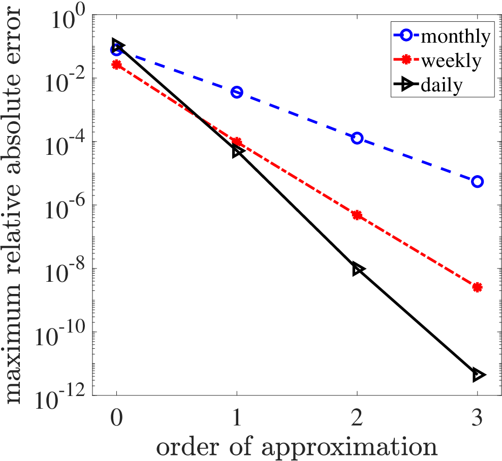
Refer to caption (a) Pure jump OU model. Refer to caption (b) Constant diffusion model. Refer to caption (c) Square-root diffusion model.
Figure 1: Maximum relative absolute errors of density approximation for Models 1, 2 and 3 with orders M=0,1,2,3M=0,1,2,3.

In Figures 2, 3 and 4, we plot the series of approximation errors defined by (83) for the three models respectively. For each model, we consider the case of Δ=1/52\Delta=1/52 and denote by e0,e1,e2,e3e_{0},e_{1},e_{2},e_{3} the abbreviation of eM(Δ,x|x0;θ)e_{M}\left(\left.\Delta,x\right|x_{0};\theta\right) in (83) for M=0,1,2,3M=0,1,2,3 respectively. We observe from Figures 2 – 4 that the approximation errors decrease quickly and consistently as the order of expansion increases.

Refer to caption (a) e0e_{0}. Refer to caption (b) e1e_{1}. Refer to caption (b) e2e_{2}. Refer to caption (c) e3e_{3}.
Figure 2: Errors of density approximation for weekly monitoring frequency (Δ=1/52\Delta=1/52) in pure jump OU model, i.e., e0,e1,e2,e3e_{0},e_{1},e_{2},e_{3} as the approximation errors with respect to the expansion orders M=0,1,2,3M=0,1,2,3 respectively.
Refer to caption (a) e0e_{0}. Refer to caption (b) e1e_{1}. Refer to caption (b) e2e_{2}. Refer to caption (c) e3e_{3}.
Figure 3: Errors of density approximation for weekly monitoring frequency (Δ=1/52\Delta=1/52) in constant diffusion model, i.e., e0,e1,e2,e3e_{0},e_{1},e_{2},e_{3} as the approximation errors with respect to the expansion orders M=0,1,2,3M=0,1,2,3 respectively.
Refer to caption (a) e0e_{0}. Refer to caption (b) e1e_{1}. Refer to caption (b) e2e_{2}. Refer to caption (c) e3e_{3}.
Figure 4: Errors of density approximation for weekly monitoring frequency (Δ=1/52\Delta=1/52) in square-root diffusion model, i.e., e0,e1,e2,e3e_{0},e_{1},e_{2},e_{3} as the approximation errors with respect to the expansion orders M=0,1,2,3M=0,1,2,3 respectively.

The advantages of our asymptotic expansion method over the method of inverse Fourier transform can be summarized as follows:

(1)

When the solution of SDE (11) does not admit an explicit expression of X⁡(t)X(t) or characteristic function ϕ⁡(t,ω)\phi\left(t;\omega\right), our method can still be used to approximate the transition density.

(2)

The approximation errors decrease quickly as the approximation order MM in (35) increases, thus it suffices to use the first several expansion terms for the approximation.

(3)

Since the SDE driven by gamma process involves the fat-tail characteristic, the characteristic function ϕ⁡(t,ω)\phi\left(t;\omega\right) for the pure jump SDE decreases slowly when ω→+∞\omega\rightarrow+\infty, which induces heavy computation burden in the inverse Fourier transform method. In contrast, our expansion terms for the pure jump SDE can achieve quick convergence and be evaluated in a few seconds for any rational initial value of X0X_{0}.

5 Concluding remarks

In this paper, we propose a closed-form asymptotic expansion to approximate the transition density of the jump-diffusion SDE driven by the gamma process. We employ three examples with known characteristic functions for numerical illustrations and comparisons. Compared with the method of calculating the transition density by inverse Fourier transform of the characteristic function, our method is more efficient while achieving low approximation errors. In terms of the applications in financial engineering, our approximation method can be directly applied for option pricing and hedging to obtain analytically tractable results, which is left for further study.

Acknowledgements

Jiang and Yang’s research was supported by the National Natural Science Foundation of China (Grants No. 11671021).

References

  • Abate and Whitt (1992) Abate, J., Whitt, W., 1992. The Fourier-series method for inverting transforms of probability distributions. Queueing Systems 10, 5–88.
  • Applebaum (2009) Applebaum, D., 2009. Lévy Processes and Stochastic Calculus. Cambridge University Press.
  • Barndorff-Nielsen et al. (2001) Barndorff-Nielsen, O. E., Mikosch, T., Resnick, S. I., 2001. Lévy Processes: Theory and Applications. Springer Science & Business Media, Boston:Birkhäuser.
  • Barndorff-Nielsen and Shephard (2001a) Barndorff-Nielsen, O. E., Shephard, N., 2001a. Non-Gaussian Ornstein–Uhlenbeck-based models and some of their uses in financial economics. Journal of the Royal Statistical Society, B (Statistical Methodology) 63, 167–241.
  • Cont and Tankov (2004) Cont, R., Tankov, P., 2004. Financial Modelling with Jump Processes. Chapman and Hall, London.
  • Eberlein et al. (2013) Eberlein, E., Madan, D., Pistorius, M., Yor, M., 2013. A simple stochastic rate model for rate equity hybrid products. Applied Mathematical Finance 20, 461–488.
  • Hayashi (2008) Hayashi, M., 2008. Asymptotic expansions for functionals of a Poisson random measure. Journal of Mathematics of Kyoto University 48 (1), 91–132.
  • Hayashi and Ishikawa (2012) Hayashi, M., Ishikawa, Y., 2012. Composition with distributions of Wiener-Poisson variables and its asymptotic expansion. Mathematische Nachrichten 285, 619–658.
  • Ishikawa (2013) Ishikawa, Y., 2013. Stochastic Calculus of Variations for Jump Processes. Walter De Gruyter, Berlin.
  • James et al. (2013) James, L. F., Kim, D., Zhang, Z., 2013. Exact simulation pricing with gamma processes and their extensions. Journal of Computational Finance 17, 3–39.
  • James et al. (2017) James, L. F., Müller, G., Zhang, Z., 2017. Stochastic volatility models based on OU-gamma time change: Theory and estimation. Journal of Business & Economic Statistics 36, 1–13.
  • Jeanblanc et al. (2009) Jeanblanc, M., Yor, M., Chesney, M., 2009. Mathematical Methods for Financial Markets. Springer-Verlag.
  • Kanwal (2004) Kanwal, R. P., 2004. Generalized Functions: Theory and Applications, 3rd Edition. Birkhäuser.
  • Kawai and Takeuchi (2010) Kawai, R., Takeuchi, A., 2010. Sensitivity analysis for averaged asset price dynamics with gamma processes. Statistics & Probability Letters 80 (1), 42–49.
  • Kawai and Takeuchi (2011) Kawai, R., Takeuchi, A., 2011. Greeks formulas for an asset price model with gamma processes. Mathematical Finance 21 (4), 723–742.
  • Kloeden and Platen (1992) Kloeden, P., Platen, E., 1992. Numerical Solutions of Stochastic Differential Equations. Springer-Verlag, Berlin.
  • Kohatsu-Higa and Takeuchi (2019) Kohatsu-Higa, A., Takeuchi, A., 2019. Jump SDEs and the Study of Their Densities. Springer, Singapore.
  • Kunita (2019) Kunita, H., 2019. Stochastic Flows and Jump-Diffusions. Springer, Singapore.
  • Li (2013b) Li, C., 2013b. Maximum-likelihood estimation for diffusion processes via closed-form density expansions. Annals of Statistics 41, 1350–1380.
  • Li and Chen (2016) Li, C., Chen, D., 2016. Estimating jump–diffusions using closed-form likelihood expansions. Journal of Econometrics 195 (1), 51–70.
  • Madan et al. (1998) Madan, D. B., Carr, P. P., Chang, E. C., 1998. The variance gamma process and option pricing. European Finance Review 2 (1), 79–105.
  • Madan and Seneta (1990) Madan, D. B., Seneta, E., 1990. The variance gamma (VG) model for share market returns. Journal of Business 63 (4), 511–524.
  • Platen and Bruti-Liberati (2010) Platen, E., Bruti-Liberati, N., 2010. Numerical Solution of Stochastic Differential Equations with Jumps in Finance. Springer-Verlag, Berlin.
  • Ribeiro and Webber (2004) Ribeiro, C., Webber, N., 2004. Valuing path-dependent options in the variance-gamma model by monte carlo with a gamma bridge. Journal of Computational Finance 7 (2), 81–100.
  • Schoutens (2003) Schoutens, W., 2003. Lévy Processes in Finance: Pricing Financial Derivatives. Wiley, New York.
  • Yor (2007) Yor, M., 2007. Some remarkable properties of gamma processes. In: Advances in Mathematical Finance. Springer, pp. 37–47.