Dynamic transformation of prior knowledge into
Bayesian models for data streams

Following [25] and [46], we consider a general model $B(\beta,z,x)$ with two kinds of variables: a global variable $\beta$ of size $K\times V$ to model the latent structure that is shared among data points $x_{1:N}$, and probably a local variable $z_{i}$ to model the latent structure that governs the $i$th data point $x_{i}$.³³ 3 $V$ is the dimensionality of variable $x$, while $K$ represents the number of hidden factors. Such a model is general and successfully applied in static conditions. However, there are several challenges in a streaming environment. A data stream is an infinite sequence of minibatches $D=\{D^{1},D^{2},...,D^{t},...\}$, and each minibatch $t$ consists of $M$ observed data points: $D^{t}=\{x_{1}^{t},x_{2}^{t},...,x_{M}^{t}\}$.

Assume we have an external knowledge $\eta$ which is represented by a matrix of size $L\times V$, where $L$ is the embedding size. Note that a matrix can help us represent different kinds of knowledge in practice, such as pre-trained word embedding [47] which uses a vector to represent the meaning of a word, the relationships among entities, and social graphs for the connections of people. For example, the prior knowledge can come from graphs⁴⁴ 4 Clearly, those graphs can be represented by adjacent matrices. [48] further showed that we can represent any general graph knowledge into embedding spaces. The low rank matrices in the embedding spaces help to exploit the knowledge in the graph more effective. such as WordNet of size $V\times V$ which means $L=V$, or from word embeddings of size $E\times V$ where $E$ is the embedding dimensionality.

In practice, the prior knowledge representations and model’s variables probably have different shapes, i.e., the model parameter $\beta$ has size $K\times V$ and the prior has size $L\times V$. For this problem, we create a mapping $f$ to transform the knowledge $\eta$ into $\beta$ in each minibatch $t$.⁵⁵ 5 The mapping can be chosen as a (pre-specified) nonlinear function, a neural network,… As an example, we will use the standard softmax function as the mapping $f$ in the later subsections. This $f$ will map the linear transformation $\pi^{t}\eta$ into the space of $\beta$, where $\pi^{t}$ is a transformation matrix of size $K\times L$. Then, the global variable $\beta^{t}$ at time $t$ is computed by: $\beta^{t}=f(\pi^{t}\eta)$.

There may be a dynamic of $\beta$ over time in the data stream (e.g. the theme of tweets can significantly change from 2019 to 2020). We need to model such a dynamic, and our reparameterization before translates the dynamic into $\pi$. Therefore, we make a relation between $\pi^{t-1}$ and $\pi^{t}$ to capture such a dynamic. We assume $\pi^{t}_{k}\sim\mathcal{N}(\pi^{t-1}_{k},\sigma I)$, where $k$ is the row index of $\pi^{t}$, $I$ is the identity matrix of size $L$, and $\sigma(\geq 0$) is the variance parameter to make $\pi^{t}_{k}$ fluctuate around $\pi^{t-1}_{k}$. By this way, the sequence of transformation matrices composes a discrete-time martingale. $\pi^{t}_{k}$ can also be interpreted as a Gaussian random walk. Note that $\pi^{t}$ plays as weighting the knowledge before transformed into the global variable of the Bayesian model. The employment of a random walk help TPS exploit the knowledge $\eta$ dynamically.

Given the global variable $\beta^{t}$ in each minibatch $t$, the generative model of data points is the same as those in the original $B$. The graphical representation of TPS appears in Figure 1a.

Learning in TPS: When facing with sequential data, many approaches [38] often formulate the learning as the Bayesian filtering problem for which one has to estimate the posterior $p(\pi^{1},\pi^{2},...,\pi^{t}|D^{1},D^{2},...,D^{t})$ or $p(\pi^{t}|D^{1},D^{2},...,D^{t})$. Note that estimating one of those posteriors will require all past data, and thus is impractical for data streams, as $t\rightarrow\infty$. Here we propose an entirely different approach which avoids reusing past data. The learning process is performed in each minibatch $t$ by maximizing the posterior $p(z,\pi^{t}|\pi^{t-1},\eta,D^{t})$, where $\pi^{t-1}$ is made available from the previous minibatch. Hence, our approach will be potentially more efficient and truly applicable to data streams. We will decompose the posterior into components in order to reuse the inference steps of the original model $B$ as: $p(z,\pi^{t}|\pi^{t-1},\eta,D^{t})\propto p(z,\pi^{t},D^{t}|\pi^{t-1},\eta)\propto p(\pi^{t}|\pi^{t-1})p(z,D^{t}|\eta,\pi^{t})\propto p(\pi^{t}|\pi^{t-1})p(z,D^{t}|\beta^{t}).$

In $\log$ form, we have:

The learning process is separated into two parts for local and global variables, respectively. While the inference of local variables $(z,x)$ is inherited from the original model $B$ (e.g., by maximizing or sampling from $p(z,x|\beta^{t})$), we focus on maximizing $\mathrm{LP}$ w.r.t. $\pi^{t}$. We extract the component $G(\beta^{t})=G(f(\pi^{t}\eta))$, that contains $\beta^{t}$, from $\log p(D^{t},z|\beta^{t})$. Then, we obtain the objective function $\mathrm{LP}(\pi^{t})=\log p(\pi^{t}|\pi^{t-1})+G(f(\pi^{t}\eta))$, and maximize it by using gradient ascent. Algorithm 1 briefly describes the learning process.

Next we discuss how to apply TPS to LDA [31], one of the most popular Bayesian models. LDA consists of two global variables $(\beta,\alpha)$: $\alpha$ contributes to the topic mixture $\theta$ of each document and is fixed in this case study, and $\beta=(\beta_{1},\beta_{2},...,\beta_{K})$ where each $\beta_{k}$ is the topic distribution over $V$ words.

Suppose that there is an available prior knowledge $\eta$ of size $L\times V$. We incorporate the prior knowledge into $\beta$ by a linear transformation with a transformation matrix $\pi$ of size $K\times L$, and then followed by the softmax operator. The generative process of the documents in minibatch $t^{th}$ is as follows (Figure 1b):

1. 1.

   Draw the transformation matrix:
   $\pi_{k}^{t}\sim\mathcal{N}(\pi_{k}^{t-1},\sigma^{2}I)$

2. 2.

   Calculate the topic distributions:
   $\beta_{k}=\mathrm{softmax}({\pi_{k}^{t}}{\eta}),k\in[K]$

3. 3.

   For each document $d$ of length $N_{d}$:

   1. (a)

      Draw a mixture: $\theta_{d}\sim\mathrm{Dirichlet}(\alpha)$

   2. (b)

      For the $i^{th}$ word of $d$: Draw topic index $z_{i}\sim\mathrm{Multinomial}(\theta_{d})$ and then draw word $w_{i}\sim\mathrm{Multinomial}(\beta_{z_{i}})$

Learning parameters: We apply Algorithm 1 for estimating the posterior. We emphasize that our framework utilizes the available inference methods (e.g., variational inference, Gibbs sampling) for local variables $(w,\theta,z)$ in the original LDA model.

Here, we use mean-field variational inference as in the original paper [31]: $q(\theta_{d},z_{d}|\gamma_{d},\phi_{d})={q(\theta_{d}|\gamma)}{\prod_{n=1}^{N_{d}}{q(z_{dn}|\phi_{dn})}}$ with the variational distributions: $q(\theta_{d}|\gamma_{d})=\mathrm{Dirichlet}(\gamma_{d})$ and $q(z_{dn}|\phi_{dn})=\mathrm{Multinomial}(\phi_{dn})$ where $\gamma_{d}$ and $\phi_{d}$ are variational parameters w.r.t. document $d$. According to [31], the inference for document $d$ reduces to repeating the following updates until convergence:

where $[V]=\{1,...,V\}$, $I$ is the indicator function, $\psi$ is the digamma function, $k\in[K]$.

The component depending on the global variable $\pi_{k}^{t}$ in (1) for each $k$ given data $D^{t}$ is: $\mathrm{LP}(\pi_{k}^{t})=\sum_{d\in D^{t}}\sum_{n\in[N_{d}]}\log p(w_{dn}|z_{dn},\beta)+\log p(\pi_{k}^{t}|\pi_{k}^{t-1})=-\frac{1}{2\sigma}\parallel\pi^{t}_{k}-\pi^{t-1}_{k}\parallel^{2}_{2}+\sum_{d\in D^{t}}\sum_{n\in[N_{d}],v\in[V]}\phi_{dnk}I[w_{dn}=v]\log\beta_{kv}$, after removing some constants. In more details,

Consider the concavity of function $\mathrm{LP}(\pi_{k}^{t})$. It is obvious that $-\frac{1}{2\sigma}\parallel\pi^{t}_{k}-\pi^{t-1}_{k}\parallel^{2}_{2}$ and ${\pi_{k}^{t}}\eta_{v}$ are concave functions with respect to $\pi_{k}^{t}$. Further, the log-sum-exp function is well-known convex. Therefore, $\mathrm{LP}(\pi_{k}^{t})$ is concave with respect to $\pi_{k}^{t}$, and we can use gradient ascent to find its maximum. We can sum up the learning algorithm of TPS for LDA as in Algorithm 2.

In this subsection, we apply TPS to Multinomial Naive Bayes for classification on document streams. Let $C$ be the number of classes, $\beta_{c}$ be the class distribution over $V$ words of the vocabulary (where $\beta_{cj}=P(j|c)$ and $\sum_{j\in[V]}\beta_{cj}=1$) for each $c\in[C]$. Each document $d$ belonging to class (label) $c_{d}$ is represented by a bag of $N_{d}$ words and each word $w_{d,i}$ is generated from $\mathrm{Multinomial}(\beta_{c_{d}})$.

Suppose that we have a prior knowledge $\eta$ of size ${L\times V}$. The generative process of documents in the minibatch $t^{th}$ is as follows: For each class $c$, draw $\pi_{c}^{t}\sim\mathcal{N}(\pi_{c}^{t-1},\sigma^{2}I)$ and calculate $\beta_{c}=\mathrm{softmax}({\pi_{c}^{t}}{\eta})$. Generate document $d$ by drawing class label $c_{d}\sim\mathrm{Multinomial}(\alpha)$ and then drawing each word $w_{dn}\sim\mathrm{Multinomial}(\beta_{c_{d}})$.

Learning: From (1), we extract the term associated with $\pi_{c}^{t}$ for each class $c$ as:

where $D_{c}^{t}$ denotes the documents with class label $c$ in minibatch $t$. Learning for NB is really simple. At each minibatch $t$, we use gradient ascent to maximize $\mathrm{LP}(\pi_{c}^{t})$ with respect to $\pi_{c}^{t}$, for each $c$. $\alpha=\frac{1}{C}$ is used in our experiments.

The ability to balance the old and new knowledge is the basic requirement for a learning system. When learning from data streams, three main sources of knowledge should be considered: the old knowledge learned in past data, the new knowledge to be learned from incoming data, and the external knowledge. TPS has a simple mechanism to balance those three sources, owing to the objective function in (1):

The first term controls the flexibility of the new model. An increase in variance $\sigma$ implies that the new model at time $t$ might be far from the previous one, and thus the new model is searched in a larger region. As $\sigma\rightarrow\infty$, TPS will not remember what have been learned before. In contrast, a decrease in $\sigma$ implies the new model should not be far from the previous one. As $\sigma=0$, we cannot learn any new knowledge at all since the first term dominates $\mathrm{LP}(z,\pi^{t}_{k})$.

The second term, $\log p(z,D^{t}|\beta^{t})$, enables TPS to learn new knowledge from new data. Different with the static use of external knowledge in KPS [42], TPS exploits the prior dynamically owing to the use of the transformation matrix $\pi^{t}$. Estimation of $\pi^{t}$ at each minibatch implies the dynamic balancing between the prior and the new knowledge learned from the data at time $t$. Note that the variance $\sigma$ also plays the key role in this balance: lower $\sigma$ means less knowledge can be learned from new data. From those observations, one can see that TPS provides a simple mechanism ($\sigma$) to dynamically balance three sources of knowledge, overcoming the limitation of existing methods.

A serious issue in many learning methods is catastrophic forgetting [49], i.e., the learned knowledge can be forgotten quickly as learning from more data/tasks. This issue has been found repeatedly for neural networks, but was unclear for Bayesian models. More importantly, existing works did not theoretically show how fast a method can forget. Here, we show that SVB [24] has a fast forgetting rate. The detailed proof appears in Appendix B.

It can be shown that this property of SVB holds for Naive Bayes and a large class of LDA-based variants which are conjugate. Such a forgetting rate in SVB is much faster than the rate $\Theta(t^{-0.67})$ in human [28]. We conjecture that a fast rate might appear in many existing methods. In contrast, TPS does not encounter this problem. It has an explicit mechanism to balance the three sources of knowledge as discussed in the last subsection. By manipulating $\sigma$, TPS can remember the knowledge better.

We first evaluate TPS when applied to LDA. We take four state-of-the-art baselines: SVB [24], PVB [25], SVB-PP [26], and KPS [42].⁶⁶ 6 SVB-HPP is not included since its application to LDA requires non-trivial efforts. Further, as observed by [26], SVB-HPP is often comparable to the best SVB-PP.
Except KPS, all of SVB, PVB, and SVB-PP do not explicitly exploit external/human knowledge and can only use the prior $(\eta)$ at the initialization. Therefore, for a fair comparison, we encode the external knowledge in the initialization of those baselines. Whenever the forms of prior knowledge are unsuitable for the baselines, we use PCA to transform the edge matrices to the same shape with $\eta$.

Datasets: We use 2 regular text (Grolier, TMN) and 4 short text datasets with some statistics in Table I.⁷⁷ 7 Grolier from http://cs.nyu.edu/$\sim$roweis/data.html, TMN from http://acube.di.unipi.it/tmn-dataset/, NYT-title from http://archive.ics.uci.edu/ml/datasets/Bag+of+Words/; Yahoo-title, TagMyNews-title (TMN-title), Irishtimes from http://www.kaggle.com/therohk/ireland-historical-news/ Those short text corpora contain documents of extremely short length, and are used in our evaluation to help us see the role of prior knowledge in the cases of extreme sparsity.

Prior knowledge: We use word embedding and word graph as two kinds of prior knowledge. The word embeddings were pre-trained from 6 billion tokens of Wikipedia2014 and Gigaword5 by [50]⁸⁸ 8 http://nlp.stanford.edu/projects/glove/. Each word is represented by a $200$-dimensional vector ($L=200$).
Word graph represents the relationships among words, and is represented by a matrix of size $V\times V$. We build the $500$-nearest neighbor graph based on the cosine similarity of word embedding vectors, and utilize it as prior knowledge. Due to the high computational cost as working with a matrix of size $V\times V$, we only did experiments on Grolier and TMN-title.

Evaluation metrics: Log predictive probability (LPP) [46] and Normalized pointwise mutual information (NPMI) [32] are used. While LPP measures the generalization of a model on unseen data, NPMI examines the coherence and interpretability of the learned topics. Details about how to compute those quantities can be found in Supplement.

Settings: We simulate streaming data by dividing a dataset into a sequence of minibatches with batchsize: 500 for {Grolier, TMN, TMN-title}, 5000 for {NYT-title, Yahoo-title}. For LDA, we set $\alpha=0.01$, $K=50$ topics for {Grolier, TMN, TMN-title, Irishtimes} and $K=100$ for {NYT-title, Yahoo-title}. We use a grid search to select suitable hyperparameters for the baselines, and report the best parameter sets for each method and each dataset. The ranges of the parameters are: multiple power prior $\rho\in\{0.6,0.7,0.8,0.9,0.99\}$ for SVB-PP, population size in $\{10^{2},10^{3},10^{4},10^{5},10^{6}\}$ for PVB, dimming factor $\kappa\in\{0,0.01,0.03,0.07,0.1,0.6,0.7,0.8,0.9\}$ in KPS, and $\sigma\in\{0.01,0.1,1,10,100\}$ for TPS.

Results:

Predictive capacity: Figure 2a and Figure 3 show the results when using word embedding and word graph priors respectively. It is obvious that TPS with both kinds of prior performs significantly better than the baselines, often by a large margin. In particular, thanks to the dynamic use of prior knowledge in each minibatch, TPS keeps increasing the predictive ability when receiving more data. Moreover, TPS can attain very high predictive capacity from some beginning stages of the learning process. For regular text data, the predictive ability in the beginning minibatch is extremely higher than the baselines. This suggests that the knowledge from the prior contains a large amount of information, and TPS can exploit the knowledge better than KPS.

It is worth noticing that SVB and SVB-PP seem not to work well with extremely short text, since their predictive capability decreases as learning from more data. Short text often does not provide enough information and clear context [51, 52], and hence cause various difficulties for SVB, SVB-PP, PVB, and KPS. KPS is able to use prior knowledge, however its ability seems to be limited because its usage of the knowledge is static along the learning process. Figure 2a and Figure 3 clearly demonstrate that existing methods are prone to overfitting on short text, whereas TPS generalizes well.

Topic coherence: The results of evaluating topic coherence using NPMI are reported in Figures 2b and 3. With word embedding prior, TPS obtains the best results often with a large margin. Again, TPS is effective for short text. The information from the prior injects the knowledge of word’s relationship to the model. For using word graph prior, Figure 3 shows that TPS is stable in the best methods. Interestingly, KPS performed better than TPS for TMN-title. It seems that TPS did not exploit the full advantage of this knowledge, although its predictiveness is still the best.

The role of prior knowledge and transition model: There are two important components which can significantly affect the performance of TPS: the prior knowledge $\eta$, and the transition model ($\pi^{t}_{k}\sim\mathcal{N}(\pi^{t-1}_{k},\sigma I)$) which connects the models in two consecutive time steps. We would like to see which one is really important to the performance of TPS. To this end, we take LDA as the base model, fix batchsize = 500, $\sigma=1,K=100$, and pre-trained word embedding as prior. Figure 4a shows the performance of TPS in three versions. One can observe that when there is no prior, TPS does not perform well and even encounters overfitting in short text. When a good prior knowledge is available, TPS performs significantly better and do not encounter overfitting. The transition model plays a good role as removing it may result in worse performance. It is worth observing that TPS tends to be better as learning from more data. This suggests that the prior knowledge does not overwhelm the data, but supports TPS to learn better.

Sensitivity of $\sigma$: Grolier (regular text) and TMN-title (short text) are used in this evaluation. We fix the batchsize to $1000$ and $K=100$ topics. The results are presented in Figure 4b. This figure shows that one should use small $\sigma$ for long text, and large $\sigma$ for short text. The reason might be that short text contains little information and few changes will likely lead to a great variance in the meaning of that text. Therefore, the new model $\pi^{t}$ should be learned in a large region around $\pi^{t-1}$ to capture large variance in incoming data. This coincides well with our theoretical analysis.

We compare TPS with SVB and KPS when applied to Naive Bayes for streaming classification. We use grid search to find the best $\kappa$ in KPS. For TPS, we use $\sigma=1$.

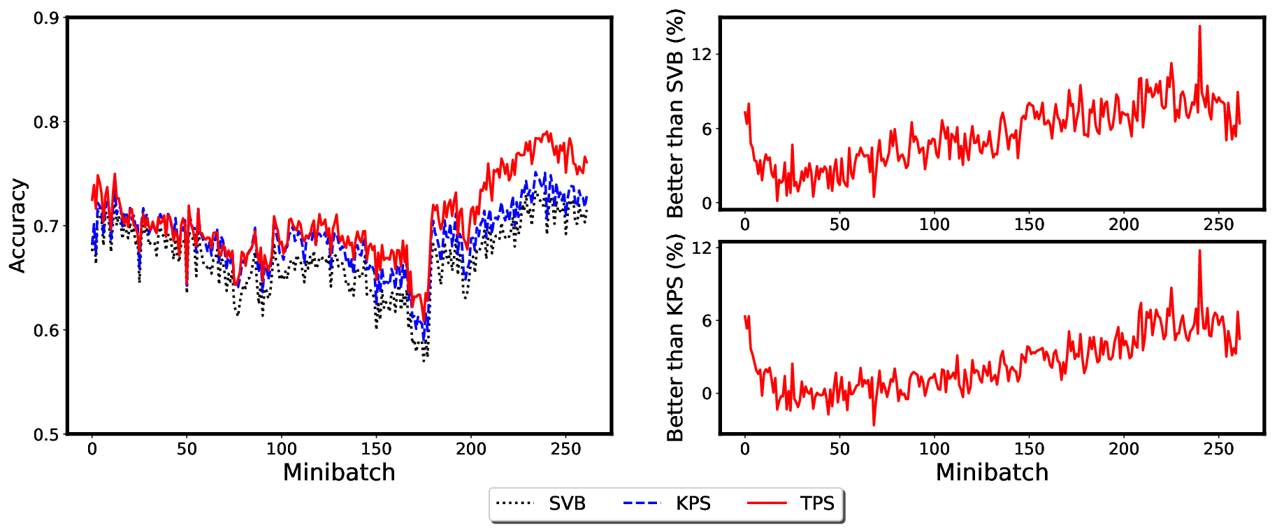
Dataset: We use Irishtimes which consists of $6$ categories (business, culture, news, opinion, sport, and letters). We continuously train a model when a minibatch arrives, then do classification for documents in the next minibatch. Here, each minibatch contains the documents of a month.

Prior knowledge: We extract a feature $V$-dimensional vector of each class $c$ whose element $j$ is the ratio of the number of word $j$ appeared in the class $c$ to the number of documents containing word $j$. Then, we gain a matrix $C\times V$ in which each term $v$ is represented by a $C$-dimensional vector. This matrix is used as prior for SVB and KPS. In TPS, we identify each word $v$ by concatenating a one-hot vector ($V$-dimension) and the $C$-dimensional vector in order to get a sufficient representation. We use this representation as prior knowledge.

Results: Figure 5 reports the accuracies of three methods. TPS is comparable to KPS in the first $100$ minibatches, better about $1-8.3\%$ than KPS in the remaining minibatches. We observe that the prior knowledge is definitely suitable for KPS as it helps KPS to obtain high accuracy. The gap between TPS and KPS is significant when the number of minibatches is large. In contrast, SVB only utilizes the knowledge at the first step, and hence often gets lower accuracy than the other methods. Note that TPS performs significantly better than both KPS and SVB in the last 100 minibatches. It is worth noting that at some sudden changes in the data distribution, the performance of SVB and KPS drops significantly. TPS can reduce such a bad effect of those sudden changes. The main reason may come from the effective exploitation of prior knowledge. This seems to be an advantage of TPS in changing environments.

The final evaluation is to see how well can the baselines utilize the full strength of external knowledge. The experiments with Naive Bayes in the previous subsection provide some good evidences as all methods can use the original knowledge. However, in the experiments with LDA in subsection V-A we have to transform the knowledge (pre-trained word embedding) into a form that can be used in SVB, SVB-PP, PVB, and KPS, due to the mismatch in dimensionality and negativity in the embedding vectors. The transformation may cause some loss in the knowledge and hence may make some bias for the baselines, since TPS uses the original knowledge representation. Next we would like to see the performance of those methods when directly using the original knowledge representation. In this case we have to match the dimensionality of the knowledge and the global variable in LDA.

We took LDA and three large datasets into evaluation: NYT-title, Yahoo-title, Irishtimes. All the settings are the same as in Subsection V-A, except that the number of topics is $K=200$ which is exactly the dimensionality of the pre-trained word embedding. To ensure non-negativity in the knowledge vectors, we normalize each embedding vector to be in $[0,1]^{200}$.

Figure 6 shows the results. We observe that the behaviors of the baselines are almost the same as in the experiments of Subsection V-A. One interesting thing is that KPS in this evaluation seems not to utilize the knowledge well, as its performance keeps steady or deteriorates over time. This is in contrast to the case where the knowledge is transformed into a lower dimensionality by PCA, and then input to the baselines. Figure 6 suggests that TPS can utilize the knowledge well to perform significantly better than the baselines in both measures.

In summary, TPS can directly exploit an external knowledge of different forms when learning a model, while other baselines find difficulties. TPS can use the knowledge in its original representation, while other methods often need a suitable transformation and hence do not well exploit the full strength of the external knowledge to improve a Bayesian model.

References

- [1] D. M. Blei, A. Kucukelbir, and J. D. McAuliffe, “Variational inference: A review for statisticians,” Journal of the American Statistical Association, vol. 112, no. 518, pp. 859–877, 2017.
- [2] G. E. P. Box, “Science and statistics,” Journal of the American Statistical Association, vol. 71, no. 356, pp. 791–799, 1976.
- [3] Z. Huang, H. Chen, and D. Zeng, “Applying associative retrieval techniques to alleviate the sparsity problem in collaborative filtering,” ACM Transactions on Information Systems (TOIS), vol. 22, no. 1, pp. 116–142, 2004.
- [4] B. Hidasi, A. Karatzoglou, L. Baltrunas, and D. Tikk, “Session-based recommendations with recurrent neural networks,” in International Conference on Learning Representations, 2016.
- [5] S. Banerjee, K. Ramanathan, and A. Gupta, “Clustering short texts using wikipedia,” in ACM SIGIR, pp. 787–788, 2007.
- [6] X. Cheng, X. Yan, Y. Lan, and J. Guo, “Btm: Topic modeling over short texts,” IEEE Transactions on Knowledge and Data Engineering, vol. 26, no. 12, pp. 2928–2941, 2014.
- [7] J. Liang, L. Jiang, D. Meng, and A. Hauptmann, “Leveraging multi-modal prior knowledge for large-scale concept learning in noisy web data,” in Proceedings of the 2017 ACM on International Conference on Multimedia Retrieval, pp. 32–40, ACM, 2017.
- [8] C. Ha, V.-D. Tran, L. Ngo, and K. Than, “Eliminating overfitting of probabilistic topic models on short and noisy text: The role of dropout,” International Journal of Approximate Reasoning, vol. 112, pp. 85–104, 2019.
- [9] D. A. Nguyen, V. L. Ngo, K. A. Nguyen, C. H. Nguyen, and K. Than, “Boosting prior knowledge in streaming variational bayes,” Neurocomputing, vol. 424, pp. 143–159, 2021.
- [10] J. Tang, Z. Meng, X. Nguyen, Q. Mei, and M. Zhang, “Understanding the limiting factors of topic modeling via posterior contraction analysis,” in Proceedings of The 31st International Conference on Machine Learning (ICML), pp. 190–198, 2014.
- [11] L. Yao, Y. Zhang, B. Wei, Z. Jin, R. Zhang, Y. Zhang, and Q. Chen, “Incorporating knowledge graph embeddings into topic modeling.,” in AAAI, pp. 3119–3126, 2017.
- [12] D. Q. Nguyen, R. Billingsley, L. Du, and M. Johnson, “Improving topic models with latent feature word representations,” Transactions of the Association for Computational Linguistics, vol. 3, pp. 299–313, 2015.
- [13] H. Zhao, L. Du, and W. Buntine, “A word embeddings informed focused topic model,” in Asian Conference on Machine Learning, pp. 423–438, 2017.
- [14] T. Ideker, J. Dutkowski, and L. Hood, “Boosting signal-to-noise in complex biology: prior knowledge is power,” Cell, vol. 144, no. 6, pp. 860–863, 2011.
- [15] D. Andrzejewski, X. Zhu, and M. Craven, “Incorporating domain knowledge into topic modeling via dirichlet forest priors,” in Proceedings of the 26th Annual International Conference on Machine Learning, pp. 25–32, ACM, 2009.
- [16] D. Andrzejewski, X. Zhu, M. Craven, and B. Recht, “A framework for incorporating general domain knowledge into latent dirichlet allocation using first-order logic,” in IJCAI, vol. 22, p. 1171, 2011.
- [17] J. Jagarlamudi, H. Daumé III, and R. Udupa, “Incorporating lexical priors into topic models,” in EACL, pp. 204–213, 2012.
- [18] Z. Chen, A. Mukherjee, B. Liu, M. Hsu, M. Castellanos, and R. Ghosh, “Leveraging multi-domain prior knowledge in topic models.,” in IJCAI, vol. 13, pp. 2071–77, 2013.
- [19] M. Sweeting, D. De Angelis, M. Hickman, and A. Ades, “Estimating hepatitis c prevalence in england and wales by synthesizing evidence from multiple data sources. assessing data conflict and model fit,” Biostatistics, vol. 9, no. 4, pp. 715–734, 2008.
- [20] S. Tan, S. Makela, D. Heller, K. Konty, S. Balter, T. Zheng, and J. H. Stark, “A bayesian evidence synthesis approach to estimate disease prevalence in hard-to-reach populations: hepatitis c in new york city,” Epidemics, vol. 23, pp. 96–109, 2018.
- [21] J. Devlin, M.-W. Chang, K. Lee, and K. Toutanova, “Bert: Pre-training of deep bidirectional transformers for language understanding,” in Proceedings of the NAACL-HLT, pp. 384–394, 2019.
- [22] D. Erhan, Y. Bengio, A. Courville, P.-A. Manzagol, P. Vincent, and S. Bengio, “Why does unsupervised pre-training help deep learning?,” Journal of Machine Learning Research, vol. 11, pp. 625–660, 2010.
- [23] J. Turian, L. Ratinov, and Y. Bengio, “Word representations: a simple and general method for semi-supervised learning,” in Proceedings of the 48th Annual Meeting of the Association for Computational Linguistics, 2010.
- [24] T. Broderick, N. Boyd, A. Wibisono, A. C. Wilson, and M. I. Jordan, “Streaming variational bayes,” in Advances in Neural Information Processing Systems, pp. 1727–1735, 2013.
- [25] J. McInerney, R. Ranganath, and D. M. Blei, “The population posterior and bayesian modeling on streams,” in Advances in Neural Information Processing Systems 28, pp. 1153–1161, 2015.
- [26] A. Masegosa, T. D. Nielsen, H. Langseth, D. Ramos-López, A. Salmerón, and A. L. Madsen, “Bayesian models of data streams with hierarchical power priors,” in Proceedings of the 34th International Conference on Machine Learning, vol. 70, pp. 2334–2343, PMLR, 2017.
- [27] M. Faraji, K. Preuschoff, and W. Gerstner, “Balancing new against old information: The role of puzzlement surprise in learning,” Neural computation, vol. 30, no. 1, pp. 34–83, 2018.
- [28] L. Averell and A. Heathcote, “The form of the forgetting curve and the fate of memories,” Journal of Mathematical Psychology, vol. 55, no. 1, pp. 25–35, 2011.
- [29] D. M. Blei and J. D. Lafferty, “Dynamic topic models,” in Proceedings of the 23rd international conference on Machine learning, pp. 113–120, ACM, 2006.
- [30] L. Charlin, R. Ranganath, J. McInerney, and D. M. Blei, “Dynamic poisson factorization,” in Proceedings of the 9th ACM Conference on Recommender Systems, pp. 155–162, ACM, 2015.
- [31] D. M. Blei, A. Y. Ng, and M. I. Jordan, “Latent dirichlet allocation,” Journal of Machine Learning Research, vol. 3, pp. 993–1022, 2003.
- [32] J. H. Lau, D. Newman, and T. Baldwin, “Machine reading tea leaves: Automatically evaluating topic coherence and topic model quality,” in EACL, pp. 530–539, 2014.
- [33] X. Wang and A. McCallum, “Topics over time: a non-markov continuous-time model of topical trends,” in Proceedings of the 12th ACM SIGKDD International Conference on Knowledge Discovery and Data Mining, pp. 424–433, ACM, 2006.
- [34] X. Wei, J. Sun, and X. Wang, “Dynamic mixture models for multiple time-series,” in IJCAI, vol. 7, pp. 2909–2914, 2007.
- [35] C. Wang, D. Blei, and D. Heckerman, “Continuous time dynamic topic models,” in Uncertainty in Artificial Intelligence, pp. 579–586, 2008.
- [36] O. Cappé and E. Moulines, “On-line expectation–maximization algorithm for latent data models,” Journal of the Royal Statistical Society: Series B (Statistical Methodology), vol. 71, no. 3, pp. 593–613, 2009.
- [37] L. Bottou, F. E. Curtis, and J. Nocedal, “Optimization methods for large-scale machine learning,” SIAM Review, vol. 60, no. 2, pp. 223–311, 2018.
- [38] A. Doucet, N. De Freitas, and N. Gordon, “An introduction to sequential monte carlo methods,” in Sequential Monte Carlo methods in practice, Springer, 2001.
- [39] J. Petterson, W. Buntine, S. M. Narayanamurthy, T. S. Caetano, and A. J. Smola, “Word features for latent dirichlet allocation,” in Advances in Neural Information Processing Systems, pp. 1921–1929, 2010.
- [40] P. Xie, D. Yang, and E. Xing, “Incorporating word correlation knowledge into topic modeling,” in NAACL-HLT, pp. 725–734, 2015.
- [41] J. G. Ibrahim, M.-H. Chen, Y. Gwon, and F. Chen, “The power prior: theory and applications,” Statistics in medicine, vol. 34, no. 28, pp. 3724–3749, 2015.
- [42] N. D. Anh, N. V. Linh, N. K. Anh, and K. Than, “Keeping priors in streaming bayesian learning,” in Advances in Knowledge Discovery and Data Mining: 21st Pacific-Asia Conference, Proceedings, Part II, pp. 247–258, Springer, 2017.
- [43] Y. He, C. Lin, W. Gao, and K.-F. Wong, “Dynamic joint sentiment-topic model,” ACM Transactions on Intelligent Systems and Technology (TIST), vol. 5, no. 1, p. 6, 2013.
- [44] P. Jähnichen, F. Wenzel, M. Kloft, and S. Mandt, “Scalable generalized dynamic topic models,” in Proceedings of the 21st International Conference on Artificial Intelligence and Statistics, vol. 84, pp. 1427–1435, PMLR, 2018.
- [45] A. B. Dieng, F. J. Ruiz, and D. M. Blei, “The dynamic embedded topic model,” arXiv preprint arXiv:1907.05545, 2019.
- [46] M. D. Hoffman, D. M. Blei, C. Wang, and J. W. Paisley, “Stochastic variational inference.,” Journal of Machine Learning Research, vol. 14, no. 1, pp. 1303–1347, 2013.
- [47] T. Mikolov, I. Sutskever, K. Chen, G. S. Corrado, and J. Dean, “Distributed representations of words and phrases and their compositionality,” in Advances in neural information processing systems, pp. 3111–3119, 2013.
- [48] A. Bordes, N. Usunier, A. Garcia-Duran, J. Weston, and O. Yakhnenko, “Translating embeddings for modeling multi-relational data,” in Advances in neural information processing systems, pp. 2787–2795, 2013.
- [49] G. I. Parisi, R. Kemker, J. L. Part, C. Kanan, and S. Wermter, “Continual lifelong learning with neural networks: A review,” Neural Networks, vol. 113, pp. 54–71, 2019.
- [50] J. Pennington, R. Socher, and C. Manning, “Glove: Global vectors for word representation,” in EMNLP, pp. 1532–1543, 2014.
- [51] L. Hong and B. D. Davison, “Empirical study of topic modeling in twitter,” in Proceedings of the first workshop on social media analytics, pp. 80–88, ACM, 2010.
- [52] X. Yan, J. Guo, Y. Lan, and X. Cheng, “A biterm topic model for short texts,” in Proceedings of the 22nd international conference on World Wide Web, pp. 1445–1456, 2013.
Appendix A Streaming Naive Bayes
In this section, we explicitly describe the application of TPS, SVB [24], and KPS [42] to multinomial Naive Bayes (NB) for classification in document streams. It is worth noting that NB models the documents in each class by a multinomial distribution with parameter . A batch learning algorithm for NB focuses mostly on estimating for a classification problem with classes.99 9 Estimating the prior for each class is important. But for simplicity, in this study we use uniform prior over class labels.
For TPS, the derivation is presented in the main paper. Algorithm 3 presents the streaming learning for NB by TPS.
Using variational inference, SVB [24] approximates the posterior distribution of in Naive Bayes by variational distribution where is the variational parameter associated with class . Therefore learning NB is translating to learning the variational parameters . Similar to the case of LDA, we update the model at time stamp by:
where comes from the previous minibatch and is initialized with prior . The learned information from the data at minibatch is inferred by variational inference as , where is the frequency of term in document . Algorithm 4 summarizes the streaming learning for NB by SVB.