跳到论文正文
W Papers独立论文阅读器 arXiv:2003.06029 论文正文 计算阅读时间 · 0%
引用这篇论文根据当前论文元数据生成,正式投稿前建议核对。


License: CC BY 4.0
arXiv:2003.06029v2 [eess.SP] 15 Jun 2020

Eigen Value Analysis in Lower Bounding Uncertainty of Kalman Filter EstimatesfootnoteinfoThis research was sponsored by Air Force Office of Scientific Research, Dynamic Data Driven Applications Systems grant FA9550-15-1-0071

Niladri Das & Raktim Bhattacharya Address: Department of Aerospace Engineering, Texas A&M University, College Station, Texas, USA. (e-mail: niladridas,raktim@tamu.edu).
Abstract

In this paper we are concerned with the error-covariance lower-bounding problem in Kalman filtering: a sensor releases a set of measurements to the data fusion/estimation center, which has a perfect knowledge of the dynamic model, to allow it to estimate the states, while preventing it to estimate the states beyond a given accuracy. We propose a measurement noise manipulation scheme to ensure lower-bound on the estimation accuracy of states. Our proposed method ensures lower-bound on the steady state estimation error of Kalman filter, using mathematical tools from eigen value analysis.

keywords
Non-linear systems, estimation, monitoring, lower-bound, optimization, privacy, eigen value analysis

1 Introduction

In various applications such as air traffic in Kirubarajan and Bar-Shalom 2003, ground traffic in Work et al. 2008, power grid in Ghahremani and Kamwa 2011, and health monitoring in Yi et al. 2013, state estimation plays in important role. Kalman filtering covers a wide variety of such applications. A Kalman filter used in any of these scenarios provides information about the accuracy of the state estimates. For an air traffic system this might be the accuracy of the GPS location, whereas for the smart grid this might be the power consumption pattern for a house-hold. These estimates rely on the measurement data shared by the user itself and might be publicly available. Publicly available measurement data can be utilized with a knowledge about the dynamics to accurately estimate states of a particular individual entity such as a house-hold power consumption pattern or states of a covert satellite.

The primary concern in each of these cases is to ensure that the measurement data can not be used by someone with exact knowledge of the dynamics to estimate the states beyond certain accuracy. The optimal strategy to ensure this is, not sharing any measurement data at all. This strategy is impractical because a user who wants privacy might be a part of the bigger network whose operation relies on data sharing. For a smart grid reliable data sharing of the house-hold consumption ensure optimal power distributions, whereas in case of satellites this ensures reduced risk of collision between two active satellites which have undergone orbit changing maneuvers.

Ruling out the possibility of not sharing any data, the problem essentially convert to the following: how can we transform the measurement data that will ensure state estimation error, using a Kalman filter, of some or all of the states to be always above a certain accuracy level ?

Contributions of the paper: On a formulation level, if the system dynamics for states 𝒙{\color[rgb]{0,0,0}\boldsymbol{x}} is: 𝒙k+1=𝑨​𝒙k+𝑩​𝒘k,∀k∈ℕ,{\color[rgb]{0,0,0}\boldsymbol{x}}_{k+1}={\color[rgb]{0,0,0}\boldsymbol{A}}{\color[rgb]{0,0,0}\boldsymbol{x}}_{k}+{\color[rgb]{0,0,0}\boldsymbol{B}}{\color[rgb]{0,0,0}\boldsymbol{w}}_{k},\ \forall k\in\mathbb{N}, and the measurement equation for measurements 𝒚{\color[rgb]{0,0,0}\boldsymbol{y}} is: 𝒚k=𝑪​𝒙k+𝒏k,∀k∈ℕ,{\color[rgb]{0,0,0}\boldsymbol{y}}_{k}={\color[rgb]{0,0,0}\boldsymbol{C}}{\color[rgb]{0,0,0}\boldsymbol{x}}_{k}+{\color[rgb]{0,0,0}\boldsymbol{n}}_{k},\ \forall k\in\mathbb{N}, whose Kalman filtering based covariance update equation is:

𝑷k|k\displaystyle{\color[rgb]{0,0,0}\boldsymbol{P}}_{k|k} =𝑷k|k−1−𝑷k|k−1​𝑪T​(𝑪​𝑷k|k−1​𝑪T+𝑹)−1\displaystyle={\color[rgb]{0,0,0}\boldsymbol{P}}_{k|k-1}-{\color[rgb]{0,0,0}\boldsymbol{P}}_{k|k-1}{\color[rgb]{0,0,0}\boldsymbol{C}}^{T}({\color[rgb]{0,0,0}\boldsymbol{C}}{\color[rgb]{0,0,0}\boldsymbol{P}}_{k|k-1}{\color[rgb]{0,0,0}\boldsymbol{C}}^{T}+{\color[rgb]{0,0,0}\boldsymbol{R}})^{-1}
×𝑪​𝑷k|k−1\displaystyle\times{\color[rgb]{0,0,0}\boldsymbol{C}}{\color[rgb]{0,0,0}\boldsymbol{P}}_{k|k-1}

where 𝑷k|k−1{\color[rgb]{0,0,0}\boldsymbol{P}}_{k|k-1} and 𝑷k|k{\color[rgb]{0,0,0}\boldsymbol{P}}_{k|k} denotes the prior and posterior covariance matrix, the question that we are interested in answering is: manipulate 𝑹{\color[rgb]{0,0,0}\boldsymbol{R}} matrix such that a certain lower-bound is satisfied. Regulating 𝑹{\color[rgb]{0,0,0}\boldsymbol{R}} is akin to adding synthetic measurement noise, deciding noise intensity for active sensors such as lidar or laser, and scheduling or selecting sensing regimes. Sensor selection techniques are covered in Singh et al. 2017,Zhang et al. 2017,and Tzoumas et al. 2016 among others.

Similar question is dealt most recently in Song et al. 2018. The authors investigate the existence of a linear transformation of the measurement space, compressing the measurement information, thus inflating the estimation error covariance. Apart from using a linear transform, we can also regulate the covariance of the steady state error estimates by adding noise to the measurements. This is the major difference between our work and the existing ones, is that we are interested in calculating the measurement noise covariance that satisfies the of lower-bound on the estimation error covariance.

Notations: Let ℕ\mathbb{N} and ℝ\mathbb{R} (ℝ+\mathbb{R}_{+}) represent the sets of natural number and real (positive real) numbers respectively. The state space of system is a closed set in ℝnx\mathbb{R}^{n_{x}}, where nxn_{x} is the dimension of the states. Transpose of a square matrix 𝐌∈ℝn×n\mathbf{M}\in\mathbb{R}^{n\times n} is denoted as 𝐌T\mathbf{M}^{T}. A positive definite (semi-definite) matrix 𝐌\mathbf{M} is denoted by 𝐌≻0\mathbf{M}\succ 0 (𝐌⪰0\mathbf{M}\succeq 0) and 𝐌≻𝑵\mathbf{M}\succ\boldsymbol{N} (𝐌⪰𝑵\mathbf{M}\succeq\boldsymbol{N}) if 𝐌−𝐍≻0\mathbf{M}-\mathbf{N}\succ 0 (𝐌−𝐍⪰0\mathbf{M}-\mathbf{N}\succeq 0), for some matrix 𝐍∈ℝn×n\mathbf{N}\in\mathbb{R}^{n\times n}. The set of all positive definite (semi-definite) matrices of size n×nn\times n is denoted by 𝑺n+⁣+{\color[rgb]{0,0,0}\boldsymbol{S}}^{++}_{n} (𝑺n+{\color[rgb]{0,0,0}\boldsymbol{S}}^{+}_{n}). Let λi​(𝐌)\lambda_{i}(\mathbf{M}) denotes ithi^{\text{th}} eigen value of the matrix 𝐌\mathbf{M}, when we arrange them as λ1​(𝐌)≥λ2​(𝐌)≥…≥λn​(𝐌)\lambda_{1}(\mathbf{M})\geq\lambda_{2}(\mathbf{M})\geq...\geq\lambda_{n}(\mathbf{M}). Similarly, singular values σi​(𝐌)\sigma_{i}(\mathbf{M}) of 𝐌\mathbf{M}, are arranged in non-increasing order: σ1​(𝐌)≥σ2​(𝐌)≥…≥σn​(𝐌)\sigma_{1}(\mathbf{M})\geq\sigma_{2}(\mathbf{M})\geq...\geq\sigma_{n}(\mathbf{M}). Let diag(𝐚\mathbf{a}) denotes a diagonal matrix, with 𝐚\mathbf{a} as its diagonal elements. We assume that 𝒙∈𝒳{\color[rgb]{0,0,0}\boldsymbol{x}}\in\mathcal{X} is continuous and μ⁡(𝒙)\mu({\color[rgb]{0,0,0}\boldsymbol{x}}) is a Lebesgue measure and p(𝒙{\color[rgb]{0,0,0}\boldsymbol{x}}) is the probability density function (pdf). The expected value of the random variable 𝒙{\color[rgb]{0,0,0}\boldsymbol{x}} with respect to p(𝒙{\color[rgb]{0,0,0}\boldsymbol{x}}) is represented as 𝔼⁡[𝒙]\mathbb{E}\left[{\color[rgb]{0,0,0}\boldsymbol{x}}\right].

Layout of the paper: The remainder of the paper is organized as follows. In Section 2, we present the system model along with its corresponding measurement model. In Section 3, we present Kalman filtering, leading to the problem statement in Section 4. In Section 5, we introduce preliminary results that lead us to the algorithm to solve the sensor covariances in section 6. In Section 7, the proposed framework is applied to a system. The paper finally concludes with Section 8.

2 System dynamics and measurement model

We focus on the class of discrete-time linear time invariant stochastic systems. Let 𝒙k{\color[rgb]{0,0,0}\boldsymbol{x}}_{k} represent the true states of a system at the kthk^{\text{th}} time instant, where 𝒙k∈ℝnx{\color[rgb]{0,0,0}\boldsymbol{x}}_{k}\in\mathbb{R}^{n_{x}} for all k∈ℕk\in\mathbb{N}. The dynamics is modeled as:

𝒙k+1=𝑨​𝒙k+𝑩​𝒘k,∀k∈ℕ,{\color[rgb]{0,0,0}\boldsymbol{x}}_{k+1}={\color[rgb]{0,0,0}\boldsymbol{A}}{\color[rgb]{0,0,0}\boldsymbol{x}}_{k}+{\color[rgb]{0,0,0}\boldsymbol{B}}{\color[rgb]{0,0,0}\boldsymbol{w}}_{k},\ \forall k\in\mathbb{N}, (1)

where 𝑨∈ℝnx×nx{\color[rgb]{0,0,0}\boldsymbol{A}}\in\mathbb{R}^{n_{x}\times n_{x}} is the state transition matrix and matrix 𝑩∈ℝnx×nw{\color[rgb]{0,0,0}\boldsymbol{B}}\in\mathbb{R}^{n_{x}\times n_{w}}. The process noise variable 𝒘k∈ℝnw{\color[rgb]{0,0,0}\boldsymbol{w}}_{k}\in\mathbb{R}^{n_{w}}, is the nwn_{w} dimensional zero-mean Gaussian additive noise with 𝔼⁡[𝒘k​𝒘lT]=𝑸​δk​l\mathbb{E}[{\color[rgb]{0,0,0}\boldsymbol{w}}_{k}{\color[rgb]{0,0,0}\boldsymbol{w}}_{l}^{T}]={\color[rgb]{0,0,0}\boldsymbol{Q}}\delta_{kl}.
The discrete dynamics in (1) is observed by a linear measurement model. Let 𝒚k∈ℝny{\color[rgb]{0,0,0}\boldsymbol{y}}_{k}\in\mathbb{R}^{n_{y}} denote the measurement taken at the kthk^{\text{th}} time instant as:

𝒚k=𝑪​𝒙k+𝒏k,∀k∈ℕ,{\color[rgb]{0,0,0}\boldsymbol{y}}_{k}={\color[rgb]{0,0,0}\boldsymbol{C}}{\color[rgb]{0,0,0}\boldsymbol{x}}_{k}+{\color[rgb]{0,0,0}\boldsymbol{n}}_{k},\ \forall k\in\mathbb{N}, (2)

where 𝒚k{\color[rgb]{0,0,0}\boldsymbol{y}}_{k} is corrupted by a nyn_{y} dimensional additive observation noise 𝒏k∈ℝnn{\color[rgb]{0,0,0}\boldsymbol{n}}_{k}\in\mathbb{R}^{n_{n}}. The sensor noise at each time instant is a zero mean Gaussian random variable with 𝔼⁡[𝒏k​𝒏lT]=𝑹​δk​l\mathbb{E}[{\color[rgb]{0,0,0}\boldsymbol{n}}_{k}{\color[rgb]{0,0,0}\boldsymbol{n}}_{l}^{T}]={\color[rgb]{0,0,0}\boldsymbol{R}}\delta_{kl}. The matrix 𝑪∈ℝny×nx{\color[rgb]{0,0,0}\boldsymbol{C}}\in\mathbb{R}^{n_{y}\times n_{x}} is known as the observation or the measurement matrix.

The initial state of (1) is modeled by a Gaussian random variable 𝒙0{\color[rgb]{0,0,0}\boldsymbol{x}}_{0} with mean 𝝁0\boldsymbol{\mu}_{0} and covariance 𝐏0\mathbf{P}_{0}. The random variable 𝒙0{\color[rgb]{0,0,0}\boldsymbol{x}}_{0} denotes the system state at the 0th0^{\text{th}} time instant. The process noise 𝒘k{\color[rgb]{0,0,0}\boldsymbol{w}}_{k}, observation noise 𝒏k{\color[rgb]{0,0,0}\boldsymbol{n}}_{k} and initial state variable 𝒙0{\color[rgb]{0,0,0}\boldsymbol{x}}_{0} are all assumed to be independent, unless otherwise specified. These assumptions are strongly motivated by analytic tractability. The restriction to zero-mean noise sources is not a loss of generality. When the noise sources are no longer zero mean, the 𝑨,𝑩{\color[rgb]{0,0,0}\boldsymbol{A}},{\color[rgb]{0,0,0}\boldsymbol{B}}, and 𝑪{\color[rgb]{0,0,0}\boldsymbol{C}} matrices are modified and extra states are introduced as shown in Anderson and Moore 1979.

3 Kalman filtering

The discrete time system in (1) and (2) induces a Kalman filter, as the optimal state estimator, with dynamics:

𝑲k\displaystyle{\color[rgb]{0,0,0}\boldsymbol{K}}_{k} =𝐏k−​𝑪T​[𝑪​𝐏k−​𝑪T+𝐑]−1,\displaystyle=\mathbf{P}_{k}^{-}{\color[rgb]{0,0,0}\boldsymbol{C}}^{T}\Big[{\color[rgb]{0,0,0}\boldsymbol{C}}\mathbf{P}_{k}^{-}{\color[rgb]{0,0,0}\boldsymbol{C}}^{T}+\mathbf{R}\Big]^{-1}, (Kalman Gain)
𝝁k−\displaystyle{\color[rgb]{0,0,0}\boldsymbol{\mu}}^{-}_{k} =𝑨​𝝁k−1+,\displaystyle={\color[rgb]{0,0,0}\boldsymbol{A}}{\color[rgb]{0,0,0}\boldsymbol{\mu}}^{+}_{k-1}, (Mean Propagation)
𝐏k−\displaystyle\mathbf{P}_{k}^{-} =𝑨​𝐏k−1+​𝑨T+𝑩​𝑸​𝑩T,\displaystyle={\color[rgb]{0,0,0}\boldsymbol{A}}\mathbf{P}^{+}_{k-1}{\color[rgb]{0,0,0}\boldsymbol{A}}^{T}+{\color[rgb]{0,0,0}\boldsymbol{B}}{\color[rgb]{0,0,0}\boldsymbol{Q}}{\color[rgb]{0,0,0}\boldsymbol{B}}^{T}, (Covariance Propagation)
𝝁k+\displaystyle{\color[rgb]{0,0,0}\boldsymbol{\mu}}^{+}_{k} =𝑨​𝝁k−1++𝑲k​(𝒚k−𝑪​𝝁k−),\displaystyle={\color[rgb]{0,0,0}\boldsymbol{A}}{\color[rgb]{0,0,0}\boldsymbol{\mu}}^{+}_{k-1}+{\color[rgb]{0,0,0}\boldsymbol{K}}_{k}({\color[rgb]{0,0,0}\boldsymbol{y}}_{k}-{\color[rgb]{0,0,0}\boldsymbol{C}}{\color[rgb]{0,0,0}\boldsymbol{\mu}}^{-}_{k}), (Mean Update)
𝐏k+\displaystyle\mathbf{P}^{+}_{k} =(𝐈−𝑲k​𝑪)​𝐏k−,\displaystyle=(\mathbf{I}-{\color[rgb]{0,0,0}\boldsymbol{K}}_{k}{\color[rgb]{0,0,0}\boldsymbol{C}})\mathbf{P}_{k}^{-}, (Covariance Update)
𝝁0+\displaystyle\boldsymbol{\mu}^{+}_{0} =𝝁0,\displaystyle=\boldsymbol{\mu}_{0}, (Initial State Mean)
𝐏0+\displaystyle\mathbf{P}^{+}_{0} =𝐏0,\displaystyle=\mathbf{P}_{0}, (Initial State Covariance)

where the variables 𝝁k−,𝝁k+∈ℝnx{\color[rgb]{0,0,0}\boldsymbol{\mu}}^{-}_{k},{\color[rgb]{0,0,0}\boldsymbol{\mu}}^{+}_{k}\in\mathbb{R}^{n_{x}}, denotes the prior and posterior mean estimate of the random variable 𝒙k{\color[rgb]{0,0,0}\boldsymbol{x}}_{k}, and 𝑲k\boldsymbol{K}_{k} is the Kalman gain, at time kk. The positive semi-definite matrices 𝐏k−,𝐏k+∈ℝnx×nx\mathbf{P}_{k}^{-},\mathbf{P}_{k}^{+}\in\mathbb{R}^{n_{x}\times n_{x}} are the prior and posterior covariance matrix at time instant kk respectively. Matrix inverse of the observation noise covariance 𝐑\mathbf{R} is defined as the precision matrix 𝑺{\color[rgb]{0,0,0}\boldsymbol{S}}.

4 Problem statement

The problem that we address is as follows: we assume that the system matrices (𝑨,𝑩,𝑪{\color[rgb]{0,0,0}\boldsymbol{A}},{\color[rgb]{0,0,0}\boldsymbol{B}},{\color[rgb]{0,0,0}\boldsymbol{C}}) and noise parameter 𝑸{\color[rgb]{0,0,0}\boldsymbol{Q}} of (1) and (2) are all known. The matrix 𝑹{\color[rgb]{0,0,0}\boldsymbol{R}} which is the sensor noise covariance, is the design variable. For a prescribed lower bound on the steady state prior covariance of the state error estimate using Kalman filter, we need to design 𝑹{\color[rgb]{0,0,0}\boldsymbol{R}} or the precision matrix 𝑺:=𝑹−1{\color[rgb]{0,0,0}\boldsymbol{S}}:={\color[rgb]{0,0,0}\boldsymbol{R}}^{-1}, that satisfies a prescribed lower-bound on the steady state error covariance.

The final result is presented as a theorem. The proof of this theorem depends upon another theorems that we first prove in the succeeding section as preliminary results.

5 Preliminaries

5.1 Preliminary results:

Middleton and Goodwin 1990 introduced the Unified Algebraic Riccati Equation :

𝑷​𝑨+𝑨T​𝑷+Δ​𝑨T​𝑷​𝑨−(Δ​𝑨T+𝑰)​𝑷​𝑩\displaystyle{\color[rgb]{0,0,0}\boldsymbol{P}}{\color[rgb]{0,0,0}\boldsymbol{A}}+{\color[rgb]{0,0,0}\boldsymbol{A}}^{T}{\color[rgb]{0,0,0}\boldsymbol{P}}+\Delta{\color[rgb]{0,0,0}\boldsymbol{A}}^{T}{\color[rgb]{0,0,0}\boldsymbol{P}}{\color[rgb]{0,0,0}\boldsymbol{A}}-(\Delta{\color[rgb]{0,0,0}\boldsymbol{A}}^{T}+{\color[rgb]{0,0,0}\boldsymbol{I}}){\color[rgb]{0,0,0}\boldsymbol{P}}{\color[rgb]{0,0,0}\boldsymbol{B}}
×(𝑰+Δ​𝑩T​𝑷​𝑩)−1​𝑩T​𝑷​(Δ​𝑨+𝑰)+𝑸=0,\displaystyle\times({{\color[rgb]{0,0,0}\boldsymbol{I}}}+\Delta{\color[rgb]{0,0,0}\boldsymbol{B}}^{T}{\color[rgb]{0,0,0}\boldsymbol{P}}{\color[rgb]{0,0,0}\boldsymbol{B}})^{-1}{\color[rgb]{0,0,0}\boldsymbol{B}}^{T}{\color[rgb]{0,0,0}\boldsymbol{P}}(\Delta{\color[rgb]{0,0,0}\boldsymbol{A}}+{\color[rgb]{0,0,0}\boldsymbol{I}})+{\color[rgb]{0,0,0}\boldsymbol{Q}}=0, (3)

where 𝑨∈ℝnx×nx{\color[rgb]{0,0,0}\boldsymbol{A}}\in\mathbb{R}^{n_{x}\times n_{x}} and 𝑩∈ℝnx×ny{\color[rgb]{0,0,0}\boldsymbol{B}}\in\mathbb{R}^{n_{x}\times n_{y}} represent constant matrices, 𝑸∈ℝnx×nx{\color[rgb]{0,0,0}\boldsymbol{Q}}\in\mathbb{R}^{n_{x}\times n_{x}} is in 𝕊n+\mathbb{S}^{+}_{n}, the matrix 𝑷∈ℝnx×nx{\color[rgb]{0,0,0}\boldsymbol{P}}\in\mathbb{R}^{n_{x}\times n_{x}} is the positive definite solution to (3), and Δ\Delta represents sampling period.

Note 1: Matrix 𝑩{\color[rgb]{0,0,0}\boldsymbol{B}} in (3) is not the same as in (1).

We introduce an extra parameter 𝑹∈ℝny×ny{\color[rgb]{0,0,0}\boldsymbol{R}}\in\mathbb{R}^{n_{y}\times n_{y}} in UARE and call it UARE-R. This UARE-R:

𝑷​𝑨+𝑨T​𝑷+Δ​𝑨T​𝑷​𝑨−(Δ​𝑨T+𝑰)​𝑷​𝑩\displaystyle{\color[rgb]{0,0,0}\boldsymbol{P}}{\color[rgb]{0,0,0}\boldsymbol{A}}+{\color[rgb]{0,0,0}\boldsymbol{A}}^{T}{\color[rgb]{0,0,0}\boldsymbol{P}}+\Delta{\color[rgb]{0,0,0}\boldsymbol{A}}^{T}{\color[rgb]{0,0,0}\boldsymbol{P}}{\color[rgb]{0,0,0}\boldsymbol{A}}-(\Delta{\color[rgb]{0,0,0}\boldsymbol{A}}^{T}+{\color[rgb]{0,0,0}\boldsymbol{I}}){\color[rgb]{0,0,0}\boldsymbol{P}}{\color[rgb]{0,0,0}\boldsymbol{B}}
×(𝑹+Δ​𝑩T​𝑷​𝑩)−1​𝑩T​𝑷​(Δ​𝑨+𝑰)+𝑸=0,\displaystyle\times({{\color[rgb]{0,0,0}\boldsymbol{R}}}+\Delta{\color[rgb]{0,0,0}\boldsymbol{B}}^{T}{\color[rgb]{0,0,0}\boldsymbol{P}}{\color[rgb]{0,0,0}\boldsymbol{B}})^{-1}{\color[rgb]{0,0,0}\boldsymbol{B}}^{T}{\color[rgb]{0,0,0}\boldsymbol{P}}(\Delta{\color[rgb]{0,0,0}\boldsymbol{A}}+{\color[rgb]{0,0,0}\boldsymbol{I}})+{\color[rgb]{0,0,0}\boldsymbol{Q}}=0, (4)

is often encountered in Optimal Control and Estimation problems such as in Bryson 2018 and Anderson and Moore 1979.

Remarks 1: (a) Using Δ=0\Delta=0, replacing 𝑨{\color[rgb]{0,0,0}\boldsymbol{A}} by 𝑨T{\color[rgb]{0,0,0}\boldsymbol{A}}^{T}, and 𝑩{\color[rgb]{0,0,0}\boldsymbol{B}} by 𝑪T{\color[rgb]{0,0,0}\boldsymbol{C}}^{T}, we recover the Continuous Time Algebraic Riccati Equation (CARE), solution to which gives us the steady state covariance for a Kalman-Bucy filter. (b) Using Δ=1\Delta=1, replacing 𝑨+𝑰{\color[rgb]{0,0,0}\boldsymbol{A}}+{\color[rgb]{0,0,0}\boldsymbol{I}} by 𝑨T{\color[rgb]{0,0,0}\boldsymbol{A}}^{T}, and 𝑩{\color[rgb]{0,0,0}\boldsymbol{B}} by 𝑪T{\color[rgb]{0,0,0}\boldsymbol{C}}^{T} we recover the Discrete Algebraic Riccati Equation (DARE) associated with steady state covariance of the Kalman Filter, where 𝑷{\color[rgb]{0,0,0}\boldsymbol{P}} denotes the steady-state error covariance matrix.

Reiterating, our objective is to design 𝑹{\color[rgb]{0,0,0}\boldsymbol{R}} matrix that satisfies prescribed lower-bound on the steady-state estimated state error covariance matrix 𝑷{\color[rgb]{0,0,0}\boldsymbol{P}}, using (4). We closely follow the calculations in Lee 2003 to relate the bounds on 𝑹{\color[rgb]{0,0,0}\boldsymbol{R}} with that of 𝑷{\color[rgb]{0,0,0}\boldsymbol{P}} in (4).

5.2 Eigen value based analysis

In the following two theorems we examine the characterization of the bounds on the 𝑷{\color[rgb]{0,0,0}\boldsymbol{P}} matrix of the UARE-R, as a function of 𝑹{\color[rgb]{0,0,0}\boldsymbol{R}}. As our final result we provide the theorem that connects the eigen values of 𝑹{\color[rgb]{0,0,0}\boldsymbol{R}} to lower bounds on 𝑷{\color[rgb]{0,0,0}\boldsymbol{P}}. This opens up a way to generate the feasible set for choosing 𝑹{\color[rgb]{0,0,0}\boldsymbol{R}} matrix.

Theorem 1

Let 𝐏{\color[rgb]{0,0,0}\boldsymbol{P}} be the positive solution of the UARE-R in equation (4), then

𝑷⪰\displaystyle{\color[rgb]{0,0,0}\boldsymbol{P}}\succeq (Δ​𝑨+𝑰)T​(𝑷l​0−1+Δ​𝑩​𝑹−1​𝑩T)−1​(Δ​𝑨+𝑰)\displaystyle(\Delta{\color[rgb]{0,0,0}\boldsymbol{A}}+{\color[rgb]{0,0,0}\boldsymbol{I}})^{T}({\color[rgb]{0,0,0}\boldsymbol{P}}_{l0}^{-1}+\Delta{\color[rgb]{0,0,0}\boldsymbol{B}}{\color[rgb]{0,0,0}\boldsymbol{R}}^{-1}{\color[rgb]{0,0,0}\boldsymbol{B}}^{T})^{-1}(\Delta{\color[rgb]{0,0,0}\boldsymbol{A}}+{\color[rgb]{0,0,0}\boldsymbol{I}})
+Δ​𝑸≡𝑷l​1\displaystyle+\Delta{\color[rgb]{0,0,0}\boldsymbol{Q}}\equiv{\color[rgb]{0,0,0}\boldsymbol{P}}_{l1} (5)

where the matrix 𝐏l​0{\color[rgb]{0,0,0}\boldsymbol{P}}_{l0} is defined as,

𝑷l​0≡\displaystyle{\color[rgb]{0,0,0}\boldsymbol{P}}_{l0}\equiv (Δ​𝑨+𝑰)T​(φ−1​𝑰+Δ​𝑩​𝑹−1​𝑩T)−1​(Δ​𝑨+𝑰)\displaystyle(\Delta{\color[rgb]{0,0,0}\boldsymbol{A}}+{\color[rgb]{0,0,0}\boldsymbol{I}})^{T}(\varphi^{-1}{\color[rgb]{0,0,0}\boldsymbol{I}}+\Delta{\color[rgb]{0,0,0}\boldsymbol{B}}{\color[rgb]{0,0,0}\boldsymbol{R}}^{-1}{\color[rgb]{0,0,0}\boldsymbol{B}}^{T})^{-1}(\Delta{\color[rgb]{0,0,0}\boldsymbol{A}}+{\color[rgb]{0,0,0}\boldsymbol{I}})
+Δ​𝑸\displaystyle+\Delta{\color[rgb]{0,0,0}\boldsymbol{Q}} (6)

and the positive constant φ\varphi is defined as,

φ≡\displaystyle\varphi\equiv f(−[λnx(𝑨+𝑨T+Δ𝑨T𝑨)+Δλnx(𝑸)λ1(𝑹−1)\displaystyle f(-[\lambda_{n_{x}}({\color[rgb]{0,0,0}\boldsymbol{A}}+{\color[rgb]{0,0,0}\boldsymbol{A}}^{T}+\Delta{\color[rgb]{0,0,0}\boldsymbol{A}}^{T}{\color[rgb]{0,0,0}\boldsymbol{A}})+\Delta\lambda_{n_{x}}({\color[rgb]{0,0,0}\boldsymbol{Q}})\lambda_{1}({\color[rgb]{0,0,0}\boldsymbol{R}}^{-1})
×σ12(𝑩)],2λ1(𝑹−1)σ12(𝑩),2λnx(𝑸)),\displaystyle\times\sigma_{1}^{2}({\color[rgb]{0,0,0}\boldsymbol{B}})],2\lambda_{1}({\color[rgb]{0,0,0}\boldsymbol{R}}^{-1})\sigma_{1}^{2}({\color[rgb]{0,0,0}\boldsymbol{B}}),2\lambda_{n_{x}}({\color[rgb]{0,0,0}\boldsymbol{Q}})), (7)

where f⁡(a,b,c)f(a,b,c) is defined as,

f⁡(a,b,c)≡−a+a2+b​cb.\displaystyle f(a,b,c)\equiv\frac{-a+\sqrt{a^{2}+bc}}{b}. (8)
{pf}

We have,

Δ⁡(𝑷​𝑨+𝑨T​𝑷+CLOSE\displaystyle\Delta({\color[rgb]{0,0,0}\boldsymbol{P}}{\color[rgb]{0,0,0}\boldsymbol{A}}+{\color[rgb]{0,0,0}\boldsymbol{A}}^{T}{\color[rgb]{0,0,0}\boldsymbol{P}}+ OPENΔ​𝑨T​𝑷​𝑨)\displaystyle\Delta{\color[rgb]{0,0,0}\boldsymbol{A}}^{T}{\color[rgb]{0,0,0}\boldsymbol{P}}{\color[rgb]{0,0,0}\boldsymbol{A}})
=\displaystyle= (Δ​𝑨+𝑰)T​𝑷​(Δ​𝑨+𝑰)−𝑷,\displaystyle(\Delta{\color[rgb]{0,0,0}\boldsymbol{A}}+{\color[rgb]{0,0,0}\boldsymbol{I}})^{T}{\color[rgb]{0,0,0}\boldsymbol{P}}(\Delta{\color[rgb]{0,0,0}\boldsymbol{A}}+{\color[rgb]{0,0,0}\boldsymbol{I}})-{\color[rgb]{0,0,0}\boldsymbol{P}}, (9)

Re-writing UARE-R as:

Δ⁡(𝑷​𝑨+𝑨T​𝑷+Δ​𝑨T​𝑷​𝑨)−Δ⁡(Δ​𝑨T+𝑰)\displaystyle\Delta({\color[rgb]{0,0,0}\boldsymbol{P}}{\color[rgb]{0,0,0}\boldsymbol{A}}+{\color[rgb]{0,0,0}\boldsymbol{A}}^{T}{\color[rgb]{0,0,0}\boldsymbol{P}}+\Delta{\color[rgb]{0,0,0}\boldsymbol{A}}^{T}{\color[rgb]{0,0,0}\boldsymbol{P}}{\color[rgb]{0,0,0}\boldsymbol{A}})-\Delta(\Delta{\color[rgb]{0,0,0}\boldsymbol{A}}^{T}+{\color[rgb]{0,0,0}\boldsymbol{I}})
×𝑷​𝑩​(𝑹+Δ​𝑩T​𝑷​𝑩)−1​𝑩T​𝑷​(Δ​𝑨+𝑰)+𝑸=0,\displaystyle\times{\color[rgb]{0,0,0}\boldsymbol{P}}{\color[rgb]{0,0,0}\boldsymbol{B}}({{\color[rgb]{0,0,0}\boldsymbol{R}}}+\Delta{\color[rgb]{0,0,0}\boldsymbol{B}}^{T}{\color[rgb]{0,0,0}\boldsymbol{P}}{\color[rgb]{0,0,0}\boldsymbol{B}})^{-1}{\color[rgb]{0,0,0}\boldsymbol{B}}^{T}{\color[rgb]{0,0,0}\boldsymbol{P}}(\Delta{\color[rgb]{0,0,0}\boldsymbol{A}}+{\color[rgb]{0,0,0}\boldsymbol{I}})+{\color[rgb]{0,0,0}\boldsymbol{Q}}=0, (10)

and using (9),

(Δ​𝑨+𝑰)T​[𝑷−Δ​𝑷​𝑩​(𝑹+Δ​𝑩T​𝑷​𝑩)−1​𝑩T​𝑷]\displaystyle(\Delta{\color[rgb]{0,0,0}\boldsymbol{A}}+{\color[rgb]{0,0,0}\boldsymbol{I}})^{T}[{\color[rgb]{0,0,0}\boldsymbol{P}}-\Delta{\color[rgb]{0,0,0}\boldsymbol{P}}{\color[rgb]{0,0,0}\boldsymbol{B}}({{\color[rgb]{0,0,0}\boldsymbol{R}}}+\Delta{\color[rgb]{0,0,0}\boldsymbol{B}}^{T}{\color[rgb]{0,0,0}\boldsymbol{P}}{\color[rgb]{0,0,0}\boldsymbol{B}})^{-1}{\color[rgb]{0,0,0}\boldsymbol{B}}^{T}{\color[rgb]{0,0,0}\boldsymbol{P}}]
×(Δ​𝑨+𝑰)+Δ​𝑸=𝑷.\displaystyle\times(\Delta{\color[rgb]{0,0,0}\boldsymbol{A}}+{\color[rgb]{0,0,0}\boldsymbol{I}})+\Delta{\color[rgb]{0,0,0}\boldsymbol{Q}}={\color[rgb]{0,0,0}\boldsymbol{P}}. (11)

Using Matrix Inversion lemma we get,

(Δ​𝑨+𝑰)T​(𝑷−1+Δ​𝑩​𝑹−1​𝑩T)−1​(Δ​𝑨+𝑰)\displaystyle(\Delta{\color[rgb]{0,0,0}\boldsymbol{A}}+{\color[rgb]{0,0,0}\boldsymbol{I}})^{T}({\color[rgb]{0,0,0}\boldsymbol{P}}^{-1}+\Delta{\color[rgb]{0,0,0}\boldsymbol{B}}{\color[rgb]{0,0,0}\boldsymbol{R}}^{-1}{\color[rgb]{0,0,0}\boldsymbol{B}}^{T})^{-1}(\Delta{\color[rgb]{0,0,0}\boldsymbol{A}}+{\color[rgb]{0,0,0}\boldsymbol{I}})
+Δ​𝑸=𝑷.\displaystyle+\Delta{\color[rgb]{0,0,0}\boldsymbol{Q}}={\color[rgb]{0,0,0}\boldsymbol{P}}. (12)

Following Lee 2003 we have,

𝑷−1\displaystyle{\color[rgb]{0,0,0}\boldsymbol{P}}^{-1} ⪯λnx−1​(𝑷)​𝑰.\displaystyle\preceq\lambda_{n_{x}}^{-1}({\color[rgb]{0,0,0}\boldsymbol{P}}){\color[rgb]{0,0,0}\boldsymbol{I}}. (13)
𝑩​𝑹−1​𝑩T\displaystyle{\color[rgb]{0,0,0}\boldsymbol{B}}{\color[rgb]{0,0,0}\boldsymbol{R}}^{-1}{\color[rgb]{0,0,0}\boldsymbol{B}}^{T} ⪯λ1​(𝑹−1)​σ12​(𝑩)​𝑰.\displaystyle\preceq\lambda_{1}({\color[rgb]{0,0,0}\boldsymbol{R}}^{-1})\sigma_{1}^{2}({\color[rgb]{0,0,0}\boldsymbol{B}}){\color[rgb]{0,0,0}\boldsymbol{I}}. (14)

Using (13) and (14) in (12), we have:

𝑷\displaystyle{\color[rgb]{0,0,0}\boldsymbol{P}} ⪰λnx​(𝑷)1+λnx​(𝑷)​Δ​λ1​(𝑹−1)​σ12​(𝑩)​(Δ​𝑨+𝑰)T\displaystyle\succeq\frac{\lambda_{n_{x}}({\color[rgb]{0,0,0}\boldsymbol{P}})}{1+\lambda_{n_{x}}({\color[rgb]{0,0,0}\boldsymbol{P}})\Delta\lambda_{1}({\color[rgb]{0,0,0}\boldsymbol{R}}^{-1})\sigma_{1}^{2}({\color[rgb]{0,0,0}\boldsymbol{B}})}(\Delta{\color[rgb]{0,0,0}\boldsymbol{A}}+{\color[rgb]{0,0,0}\boldsymbol{I}})^{T}
×(Δ​𝑨+𝑰)+Δ​𝑸\displaystyle\times(\Delta{\color[rgb]{0,0,0}\boldsymbol{A}}+{\color[rgb]{0,0,0}\boldsymbol{I}})+\Delta{\color[rgb]{0,0,0}\boldsymbol{Q}} (15)

Lemma 1 in Lee 2003 (Amir-Moez 1956) states,

λi+j−n​(𝑨1+𝑩1)≥λj​(𝑨1)+λi​(𝑩1),i+j≥n+1,\displaystyle\lambda_{i+j-n}({\color[rgb]{0,0,0}\boldsymbol{A}}_{1}+{\color[rgb]{0,0,0}\boldsymbol{B}}_{1})\geq\lambda_{j}({\color[rgb]{0,0,0}\boldsymbol{A}}_{1})+\lambda_{i}({\color[rgb]{0,0,0}\boldsymbol{B}}_{1}),\ i+j\geq n+1,

for any symmetric matrices, 𝑨1,𝑩1∈ℝn×n{\color[rgb]{0,0,0}\boldsymbol{A}}_{1},{\color[rgb]{0,0,0}\boldsymbol{B}}_{1}\in\mathbb{R}^{n\times n} and 1≤i,j≤n1\leq i,j\leq n.
Using i=ni=n and j=nj=n we have,

λn​(𝑨+𝑩)≥λn​(𝑨1)+λn​(𝑩1).\displaystyle\lambda_{n}({\color[rgb]{0,0,0}\boldsymbol{A}}+{\color[rgb]{0,0,0}\boldsymbol{B}})\geq\lambda_{n}({\color[rgb]{0,0,0}\boldsymbol{A}}_{1})+\lambda_{n}({\color[rgb]{0,0,0}\boldsymbol{B}}_{1}). (16)

Using equation (16) in equation (15) after applying eigen value operator on equation (15), we get,

λnx​(𝑷)\displaystyle\lambda_{n_{x}}({\color[rgb]{0,0,0}\boldsymbol{P}}) ≥λnx​(𝑷)1+λnx​(𝑷)​Δ​λ1​(𝑹−1)​σ12​(𝑩)λnx[(Δ𝑨+𝑰)T\displaystyle\geq\frac{\lambda_{n_{x}}({\color[rgb]{0,0,0}\boldsymbol{P}})}{1+\lambda_{n_{x}}({\color[rgb]{0,0,0}\boldsymbol{P}})\Delta\lambda_{1}({\color[rgb]{0,0,0}\boldsymbol{R}}^{-1})\sigma_{1}^{2}({\color[rgb]{0,0,0}\boldsymbol{B}})}\lambda_{n_{x}}[(\Delta{\color[rgb]{0,0,0}\boldsymbol{A}}+{\color[rgb]{0,0,0}\boldsymbol{I}})^{T}
×(Δ𝑨+𝑰)]+Δλnx(𝑸).\displaystyle\times(\Delta{\color[rgb]{0,0,0}\boldsymbol{A}}+{\color[rgb]{0,0,0}\boldsymbol{I}})]+\Delta\lambda_{n_{x}}({\color[rgb]{0,0,0}\boldsymbol{Q}}).

Using λnx​[(Δ​𝑨+𝑰)T​(Δ​𝑨+𝑰)]=Δ​λnx​(𝑨+𝑨T+Δ​𝑨T​𝑨)+1\lambda_{n_{x}}[(\Delta{\color[rgb]{0,0,0}\boldsymbol{A}}+{\color[rgb]{0,0,0}\boldsymbol{I}})^{T}(\Delta{\color[rgb]{0,0,0}\boldsymbol{A}}+{\color[rgb]{0,0,0}\boldsymbol{I}})]=\Delta\lambda_{n_{x}}({\color[rgb]{0,0,0}\boldsymbol{A}}+{\color[rgb]{0,0,0}\boldsymbol{A}}^{T}+\Delta{\color[rgb]{0,0,0}\boldsymbol{A}}^{T}{\color[rgb]{0,0,0}\boldsymbol{A}})+1 and then rearranging we get,

Δλ1(𝑹−1)σ12(𝑩)λnx2(𝑷)−[Δλnx(𝑨+𝑨T+Δ𝑨T𝑨)\displaystyle\Delta\lambda_{1}({\color[rgb]{0,0,0}\boldsymbol{R}}^{-1})\sigma_{1}^{2}({\color[rgb]{0,0,0}\boldsymbol{B}})\lambda_{n_{x}}^{2}({\color[rgb]{0,0,0}\boldsymbol{P}})-[\Delta\lambda_{n_{x}}({\color[rgb]{0,0,0}\boldsymbol{A}}+{\color[rgb]{0,0,0}\boldsymbol{A}}^{T}+\Delta{\color[rgb]{0,0,0}\boldsymbol{A}}^{T}{\color[rgb]{0,0,0}\boldsymbol{A}})
+Δλnx(𝑸)Δλ1(𝑹−1)σ12(𝑩)]λnx(𝑷)−Δλnx(𝑸)≥0,\displaystyle+\Delta\lambda_{n_{x}}({\color[rgb]{0,0,0}\boldsymbol{Q}})\Delta\lambda_{1}({\color[rgb]{0,0,0}\boldsymbol{R}}^{-1})\sigma_{1}^{2}({\color[rgb]{0,0,0}\boldsymbol{B}})]\lambda_{n_{x}}({\color[rgb]{0,0,0}\boldsymbol{P}})-\Delta\lambda_{n_{x}}({\color[rgb]{0,0,0}\boldsymbol{Q}})\geq 0, (17)

which is of quadratic form. Hence finally,

λnx(𝑷)≥f(−[λnx(𝑨+𝑨T+Δ𝑨T𝑨)+Δλnx(𝑸)\displaystyle\lambda_{n_{x}}({\color[rgb]{0,0,0}\boldsymbol{P}})\geq f(-[\lambda_{n_{x}}({\color[rgb]{0,0,0}\boldsymbol{A}}+{\color[rgb]{0,0,0}\boldsymbol{A}}^{T}+\Delta{\color[rgb]{0,0,0}\boldsymbol{A}}^{T}{\color[rgb]{0,0,0}\boldsymbol{A}})+\Delta\lambda_{n_{x}}({\color[rgb]{0,0,0}\boldsymbol{Q}})
×λ1(𝑹−1)σ12(𝑩)],2λ1(𝑹−1)σ12(𝑩),2λnx(𝑸))≡φ,\displaystyle\times\lambda_{1}({\color[rgb]{0,0,0}\boldsymbol{R}}^{-1})\sigma_{1}^{2}({\color[rgb]{0,0,0}\boldsymbol{B}})],2\lambda_{1}({\color[rgb]{0,0,0}\boldsymbol{R}}^{-1})\sigma_{1}^{2}({\color[rgb]{0,0,0}\boldsymbol{B}}),2\lambda_{n_{x}}({\color[rgb]{0,0,0}\boldsymbol{Q}}))\equiv\varphi,

where,

f⁡(a,b,c)≡−a+a2+b​cb.\displaystyle f(a,b,c)\equiv\frac{-a+\sqrt{a^{2}+bc}}{b}. (18)

We have,

λn−1​(𝑷)≤\displaystyle\lambda_{n}^{-1}({\color[rgb]{0,0,0}\boldsymbol{P}})\leq φ−1\displaystyle\ \varphi^{-1} (19)

Using equation (19) in equation (15) we get,

𝑷\displaystyle{\color[rgb]{0,0,0}\boldsymbol{P}} ⪰(Δ​𝑨+𝑰)T​(φ−1​𝑰+Δ​𝑩​𝑹−1​𝑩T)−1\displaystyle\succeq(\Delta{\color[rgb]{0,0,0}\boldsymbol{A}}+{\color[rgb]{0,0,0}\boldsymbol{I}})^{T}(\varphi^{-1}{\color[rgb]{0,0,0}\boldsymbol{I}}+\Delta{\color[rgb]{0,0,0}\boldsymbol{B}}{\color[rgb]{0,0,0}\boldsymbol{R}}^{-1}{\color[rgb]{0,0,0}\boldsymbol{B}}^{T})^{-1}
×(Δ​𝑨+𝑰)+Δ​𝑸≡𝑷l​0\displaystyle\times(\Delta{\color[rgb]{0,0,0}\boldsymbol{A}}+{\color[rgb]{0,0,0}\boldsymbol{I}})+\Delta{\color[rgb]{0,0,0}\boldsymbol{Q}}\equiv{\color[rgb]{0,0,0}\boldsymbol{P}}_{l0} (20)

Using the lower bound 𝑷l​0{\color[rgb]{0,0,0}\boldsymbol{P}}_{l0} in (12) we get,

𝑷\displaystyle{\color[rgb]{0,0,0}\boldsymbol{P}} ⪰(Δ​𝑨+𝑰)T​(𝑷l​0−1+Δ​𝑩​𝑹−1​𝑩T)−1\displaystyle\succeq(\Delta{\color[rgb]{0,0,0}\boldsymbol{A}}+{\color[rgb]{0,0,0}\boldsymbol{I}})^{T}({\color[rgb]{0,0,0}\boldsymbol{P}}_{l0}^{-1}+\Delta{\color[rgb]{0,0,0}\boldsymbol{B}}{\color[rgb]{0,0,0}\boldsymbol{R}}^{-1}{\color[rgb]{0,0,0}\boldsymbol{B}}^{T})^{-1}
×(Δ​𝑨+𝑰)+Δ​𝑸\displaystyle\times(\Delta{\color[rgb]{0,0,0}\boldsymbol{A}}+{\color[rgb]{0,0,0}\boldsymbol{I}})+\Delta{\color[rgb]{0,0,0}\boldsymbol{Q}} (21)

Theorem 1 is similar to that of Theorem 1 of Lee 2003 but derived for UARE-R, rather than for UARE.

6 Choosing 𝑹{\color[rgb]{0,0,0}\boldsymbol{R}} to Lower-bound 𝑷{\color[rgb]{0,0,0}\boldsymbol{P}}

We discussed how we retrieve DARE:

𝑨​𝑷​𝑨T−𝑷−𝑨​𝑷​𝑪T​(𝑹+𝑪​𝑷​𝑪T)−1\displaystyle{\color[rgb]{0,0,0}\boldsymbol{A}}{\color[rgb]{0,0,0}\boldsymbol{P}}{\color[rgb]{0,0,0}\boldsymbol{A}}^{T}-{\color[rgb]{0,0,0}\boldsymbol{P}}-{\color[rgb]{0,0,0}\boldsymbol{A}}{\color[rgb]{0,0,0}\boldsymbol{P}}{\color[rgb]{0,0,0}\boldsymbol{C}}^{T}({\color[rgb]{0,0,0}\boldsymbol{R}}+{\color[rgb]{0,0,0}\boldsymbol{C}}{\color[rgb]{0,0,0}\boldsymbol{P}}{\color[rgb]{0,0,0}\boldsymbol{C}}^{T})^{-1}
×𝑪​𝑷​𝑨T+𝑸=0,\displaystyle\times{\color[rgb]{0,0,0}\boldsymbol{C}}{\color[rgb]{0,0,0}\boldsymbol{P}}{\color[rgb]{0,0,0}\boldsymbol{A}}^{T}+{\color[rgb]{0,0,0}\boldsymbol{Q}}=0,

for solving the steady-state covariance matrix 𝑷{\color[rgb]{0,0,0}\boldsymbol{P}} for Kalman filter, applying suitable substitution to the UARE-R. Conventionally, designing 𝑹{\color[rgb]{0,0,0}\boldsymbol{R}} is related to upper bounding the performance of a filter with some additional constraints. Topics like differential privacy as in Dwork et al. 2014 and bounded information exchange such as in robotics as in Butler et al. 2015 has lead to the requirement of switching between different 𝑹{\color[rgb]{0,0,0}\boldsymbol{R}} matrices to keep the performance within bounds (upper or lower), rather than just upper bounding it. In this work, we utilize Theorem 1 to propose a technique to design the measurement noise covariance matrix 𝑹{\color[rgb]{0,0,0}\boldsymbol{R}} or the precision matrix 𝑺{\color[rgb]{0,0,0}\boldsymbol{S}} such that the 𝑷{\color[rgb]{0,0,0}\boldsymbol{P}} is lower bounded. We will see in the succeeding sections that the feasible set of 𝑹{\color[rgb]{0,0,0}\boldsymbol{R}} is represented as a set of linear matrix inequality (LMI).

In deriving the following result, we first construct the feasible set of 𝑹{\color[rgb]{0,0,0}\boldsymbol{R}} that satisfies prescribed lower bound on the matrix 𝑷{\color[rgb]{0,0,0}\boldsymbol{P}}. A particular choice of 𝑹{\color[rgb]{0,0,0}\boldsymbol{R}} matrix results from an optimization problem over the set of feasible 𝑹{\color[rgb]{0,0,0}\boldsymbol{R}} for a given cost function. We use c⁡(𝑹)c({\color[rgb]{0,0,0}\boldsymbol{R}}) to represent a generic cost function.

Remarks 2: If 𝑹{\color[rgb]{0,0,0}\boldsymbol{R}} is a diagonal matrix, the cost function is essentially over the space of vector 𝝀{\color[rgb]{0,0,0}\boldsymbol{\lambda}}, that constitutes the diagonal elements of 𝑹{\color[rgb]{0,0,0}\boldsymbol{R}}.

6.1 Calculate 𝑹{\color[rgb]{0,0,0}\boldsymbol{R}}: Lower bound for steady state Kalman filtering

Using Δ=1\Delta=1, replacing 𝑨+𝑰{\color[rgb]{0,0,0}\boldsymbol{A}}+{\color[rgb]{0,0,0}\boldsymbol{I}} by 𝑨T{\color[rgb]{0,0,0}\boldsymbol{A}}^{T} and 𝑩{\color[rgb]{0,0,0}\boldsymbol{B}} by 𝑪T{\color[rgb]{0,0,0}\boldsymbol{C}}^{T} in UARE-R, we recover the Discrete Algebraic Riccati Equation (DARE) associated with steady state covariance update equation of a linear system using Kalman Filter.

We assume complete detectability of [𝑨,𝑪{\color[rgb]{0,0,0}\boldsymbol{A}},{\color[rgb]{0,0,0}\boldsymbol{C}}] and stabilizability of [𝑨,𝑩​𝑸1/2{\color[rgb]{0,0,0}\boldsymbol{A}},{\color[rgb]{0,0,0}\boldsymbol{B}}{\color[rgb]{0,0,0}\boldsymbol{Q}}^{1/2}] (Anderson and Moore 1979, pg.82) for (1) and (2). This ensure that the steady state prior covariance matrix 𝑷{\color[rgb]{0,0,0}\boldsymbol{P}} exists and is unique (for a fixed 𝑹{\color[rgb]{0,0,0}\boldsymbol{R}}) for the corresponding DARE.

Theorem 2

For a given scalar cost function c(𝐑\boldsymbol{R}) and an lower bound (1/λuf)(1/\lambda^{f}_{u}) on the spectrum of 𝐑{\color[rgb]{0,0,0}\boldsymbol{R}}, the solution 𝐑∗{\color[rgb]{0,0,0}\boldsymbol{R}}^{*}, whose spectrum is

λ(𝑹∗):={λ1≥λ2≥⋯≥λn​y−1≥λn​y},\lambda({\color[rgb]{0,0,0}\boldsymbol{R}}^{*}):=\{\lambda_{1}\geq\lambda_{2}\geq\dots\geq\lambda_{ny-1}\geq\lambda_{ny}\},

where λn​y≥(1/λuf)\lambda_{ny}\geq(1/\lambda^{f}_{u}), that satisfies a given lower bound 𝐏lf{\color[rgb]{0,0,0}\boldsymbol{P}}_{l}^{f} on the steady state prior covariance matrix 𝐏{\color[rgb]{0,0,0}\boldsymbol{P}} of Kalman filter, is given by the following optimization problem.

𝑹∗\displaystyle{\color[rgb]{0,0,0}\boldsymbol{R}}^{*} :=argmin𝑹​c​(𝑹)\displaystyle:=\underset{{\color[rgb]{0,0,0}\boldsymbol{R}}}{\mathrm{argmin}}\ c({\color[rgb]{0,0,0}\boldsymbol{R}})

Such that,

𝑹\displaystyle{\color[rgb]{0,0,0}\boldsymbol{R}} ⪰(1/λuf)​𝑰,\displaystyle\succeq(1/\lambda^{f}_{u}){\color[rgb]{0,0,0}\boldsymbol{I}},
[𝑻1𝑪T𝑪𝑹]\displaystyle\begin{bmatrix}{\color[rgb]{0,0,0}\boldsymbol{T}}_{1}&{\color[rgb]{0,0,0}\boldsymbol{C}}^{T}\\ {\color[rgb]{0,0,0}\boldsymbol{C}}&{\color[rgb]{0,0,0}\boldsymbol{R}}\end{bmatrix} ⪰0,\displaystyle\succeq 0,

where,

𝑻1≡\displaystyle{\color[rgb]{0,0,0}\boldsymbol{T}}_{1}\equiv 𝑨T(𝑷lf−𝑸)−1𝑨−𝑷l​0′−1\displaystyle{\color[rgb]{0,0,0}\boldsymbol{A}}^{T}({\color[rgb]{0,0,0}\boldsymbol{P}}_{l}^{f}-{\color[rgb]{0,0,0}\boldsymbol{Q}})^{-1}{\color[rgb]{0,0,0}\boldsymbol{A}}-{{\color[rgb]{0,0,0}\boldsymbol{P}}^{{}^{\prime}}_{l0}}^{-1}
𝑷′l​0≡\displaystyle{\color[rgb]{0,0,0}\boldsymbol{P}}^{{}^{\prime}}_{l0}\equiv 𝑨​(φ′−1​𝑰+λuf​𝑪T​𝑪)−1​𝑨T+𝑸.\displaystyle{\color[rgb]{0,0,0}\boldsymbol{A}}(\varphi^{\prime-1}{\color[rgb]{0,0,0}\boldsymbol{I}}+\lambda^{f}_{u}{\color[rgb]{0,0,0}\boldsymbol{C}}^{T}{\color[rgb]{0,0,0}\boldsymbol{C}})^{-1}{\color[rgb]{0,0,0}\boldsymbol{A}}^{T}+{\color[rgb]{0,0,0}\boldsymbol{Q}}.
φ′≡\displaystyle\varphi^{\prime}\equiv f⁡(−[λnx​(𝑨​𝑨T−𝑰)+λnx​(𝑸)​λuf​σ12​(𝑪T)]CLOSE\displaystyle f(-[\lambda_{n_{x}}({\color[rgb]{0,0,0}\boldsymbol{A}}{\color[rgb]{0,0,0}\boldsymbol{A}}^{T}-{\color[rgb]{0,0,0}\boldsymbol{I}})+\lambda_{n_{x}}({\color[rgb]{0,0,0}\boldsymbol{Q}})\lambda^{f}_{u}\sigma_{1}^{2}({\color[rgb]{0,0,0}\boldsymbol{C}}^{T})]
,2λufσ12(𝑪T),2λnx(𝑸)),\displaystyle,2\lambda^{f}_{u}\sigma_{1}^{2}({\color[rgb]{0,0,0}\boldsymbol{C}}^{T}),2\lambda_{n_{x}}({\color[rgb]{0,0,0}\boldsymbol{Q}})),
{pf}

We first take a look at Theorem 1, the lower bound theorem. The variable φ\varphi is defined as,

φ\displaystyle\varphi ≡f(−[λnx(𝑨+𝑨T+Δ𝑨T𝑨)+Δλnx(𝑸)λ1(𝑹−1)\displaystyle\equiv f(-[\lambda_{n_{x}}({\color[rgb]{0,0,0}\boldsymbol{A}}+{\color[rgb]{0,0,0}\boldsymbol{A}}^{T}+\Delta{\color[rgb]{0,0,0}\boldsymbol{A}}^{T}{\color[rgb]{0,0,0}\boldsymbol{A}})+\Delta\lambda_{n_{x}}({\color[rgb]{0,0,0}\boldsymbol{Q}})\lambda_{1}({\color[rgb]{0,0,0}\boldsymbol{R}}^{-1})
×σ12(𝑩)],2λ1(𝑹−1)σ12(𝑩),2λnx(𝑸))\displaystyle\times\sigma_{1}^{2}({\color[rgb]{0,0,0}\boldsymbol{B}})],2\lambda_{1}({\color[rgb]{0,0,0}\boldsymbol{R}}^{-1})\sigma_{1}^{2}({\color[rgb]{0,0,0}\boldsymbol{B}}),2\lambda_{n_{x}}({\color[rgb]{0,0,0}\boldsymbol{Q}}))

We notice that φ\varphi is a function of λ1​(𝑹−1)\lambda_{1}({\color[rgb]{0,0,0}\boldsymbol{R}}^{-1}). We assume that λ1​(𝑹−1)≤λuf\lambda_{1}({\color[rgb]{0,0,0}\boldsymbol{R}}^{-1})\leq\lambda^{f}_{u}, i.e. upper bounded. We define:

φ′\displaystyle\varphi^{\prime} ≡f(−[λnx(𝑨+𝑨T+Δ𝑨T𝑨)+Δλnx(𝑸)λuf\displaystyle\equiv f(-[\lambda_{n_{x}}({\color[rgb]{0,0,0}\boldsymbol{A}}+{\color[rgb]{0,0,0}\boldsymbol{A}}^{T}+\Delta{\color[rgb]{0,0,0}\boldsymbol{A}}^{T}{\color[rgb]{0,0,0}\boldsymbol{A}})+\Delta\lambda_{n_{x}}({\color[rgb]{0,0,0}\boldsymbol{Q}})\lambda^{f}_{u}
×σ12(𝑩)],2λufσ12(𝑩),2λnx(𝑸))\displaystyle\times\sigma_{1}^{2}({\color[rgb]{0,0,0}\boldsymbol{B}})],2\lambda^{f}_{u}\sigma_{1}^{2}({\color[rgb]{0,0,0}\boldsymbol{B}}),2\lambda_{n_{x}}({\color[rgb]{0,0,0}\boldsymbol{Q}}))

It can be proved that φ≥φ′\varphi\geq\varphi^{\prime}. Hence we have,

𝑷l​0⪰\displaystyle{\color[rgb]{0,0,0}\boldsymbol{P}}_{l0}\succeq (Δ​𝑨+𝑰)T​(φ−1​𝑰+Δ​λ1​(𝑹−1)​𝑩​𝑩T)−1\displaystyle(\Delta{\color[rgb]{0,0,0}\boldsymbol{A}}+{\color[rgb]{0,0,0}\boldsymbol{I}})^{T}(\varphi^{-1}{\color[rgb]{0,0,0}\boldsymbol{I}}+\Delta\lambda_{1}({\color[rgb]{0,0,0}\boldsymbol{R}}^{-1}){\color[rgb]{0,0,0}\boldsymbol{B}}{\color[rgb]{0,0,0}\boldsymbol{B}}^{T})^{-1}
×(Δ​𝑨+𝑰)+Δ​𝑸,\displaystyle\times(\Delta{\color[rgb]{0,0,0}\boldsymbol{A}}+{\color[rgb]{0,0,0}\boldsymbol{I}})+\Delta{\color[rgb]{0,0,0}\boldsymbol{Q}},
⪰\displaystyle\succeq (Δ​𝑨+𝑰)T​(φ′−1​𝑰+Δ​λuf​𝑩​𝑩T)−1\displaystyle(\Delta{\color[rgb]{0,0,0}\boldsymbol{A}}+{\color[rgb]{0,0,0}\boldsymbol{I}})^{T}(\varphi^{\prime-1}{\color[rgb]{0,0,0}\boldsymbol{I}}+\Delta\lambda^{f}_{u}{\color[rgb]{0,0,0}\boldsymbol{B}}{\color[rgb]{0,0,0}\boldsymbol{B}}^{T})^{-1}
×(Δ𝑨+𝑰)+Δ𝑸≡𝑷l​0′,\displaystyle\times(\Delta{\color[rgb]{0,0,0}\boldsymbol{A}}+{\color[rgb]{0,0,0}\boldsymbol{I}})+\Delta{\color[rgb]{0,0,0}\boldsymbol{Q}}\equiv{\color[rgb]{0,0,0}\boldsymbol{P}}^{{}^{\prime}}_{l0}, (22)

Using Theorem 1 we have,

𝑷\displaystyle{\color[rgb]{0,0,0}\boldsymbol{P}} ⪰(Δ​𝑨+𝑰)T​(𝑷l​0−1+Δ​𝑩​𝑹−1​𝑩T)−1\displaystyle\succeq(\Delta{\color[rgb]{0,0,0}\boldsymbol{A}}+{\color[rgb]{0,0,0}\boldsymbol{I}})^{T}({\color[rgb]{0,0,0}\boldsymbol{P}}_{l0}^{-1}+\Delta{\color[rgb]{0,0,0}\boldsymbol{B}}{\color[rgb]{0,0,0}\boldsymbol{R}}^{-1}{\color[rgb]{0,0,0}\boldsymbol{B}}^{T})^{-1}
×(Δ​𝑨+𝑰)+Δ​𝑸\displaystyle\times(\Delta{\color[rgb]{0,0,0}\boldsymbol{A}}+{\color[rgb]{0,0,0}\boldsymbol{I}})+\Delta{\color[rgb]{0,0,0}\boldsymbol{Q}}
⪰(Δ​𝑨+𝑰)T​(𝑷l​0′−1+Δ​𝑩​𝑹−1​𝑩T)−1\displaystyle\succeq(\Delta{\color[rgb]{0,0,0}\boldsymbol{A}}+{\color[rgb]{0,0,0}\boldsymbol{I}})^{T}({{\color[rgb]{0,0,0}\boldsymbol{P}}^{\prime}_{l0}}^{-1}+\Delta{\color[rgb]{0,0,0}\boldsymbol{B}}{\color[rgb]{0,0,0}\boldsymbol{R}}^{-1}{\color[rgb]{0,0,0}\boldsymbol{B}}^{T})^{-1}
×(Δ​𝑨+𝑰)+Δ​𝑸.\displaystyle\times(\Delta{\color[rgb]{0,0,0}\boldsymbol{A}}+{\color[rgb]{0,0,0}\boldsymbol{I}})+\Delta{\color[rgb]{0,0,0}\boldsymbol{Q}}.

Now suppose we want to lower bound 𝑷{\color[rgb]{0,0,0}\boldsymbol{P}} by 𝑷lf{\color[rgb]{0,0,0}\boldsymbol{P}}_{l}^{f}. That is ensured if we have,

𝑷⪰\displaystyle{\color[rgb]{0,0,0}\boldsymbol{P}}\succeq (Δ​𝑨+𝑰)T​(𝑷l​0′−1+Δ​𝑩​𝑹−1​𝑩T)−1\displaystyle(\Delta{\color[rgb]{0,0,0}\boldsymbol{A}}+{\color[rgb]{0,0,0}\boldsymbol{I}})^{T}({{\color[rgb]{0,0,0}\boldsymbol{P}}^{\prime}_{l0}}^{-1}+\Delta{\color[rgb]{0,0,0}\boldsymbol{B}}{\color[rgb]{0,0,0}\boldsymbol{R}}^{-1}{\color[rgb]{0,0,0}\boldsymbol{B}}^{T})^{-1}
×(Δ​𝑨+𝑰)+Δ​𝑸⪰𝑷lf.\displaystyle\times(\Delta{\color[rgb]{0,0,0}\boldsymbol{A}}+{\color[rgb]{0,0,0}\boldsymbol{I}})+\Delta{\color[rgb]{0,0,0}\boldsymbol{Q}}\succeq{\color[rgb]{0,0,0}\boldsymbol{P}}_{l}^{f}.

If we assume that the (Δ​𝑨+𝑰)(\Delta{\color[rgb]{0,0,0}\boldsymbol{A}}+{\color[rgb]{0,0,0}\boldsymbol{I}}) matrix is invertible we have,

(Δ​𝑨+𝑰)−T\displaystyle(\Delta{\color[rgb]{0,0,0}\boldsymbol{A}}+{\color[rgb]{0,0,0}\boldsymbol{I}})^{-T} (𝑷lf−Δ​𝑸)​(Δ​𝑨+𝑰)−1\displaystyle({\color[rgb]{0,0,0}\boldsymbol{P}}_{l}^{f}-\Delta{\color[rgb]{0,0,0}\boldsymbol{Q}})(\Delta{\color[rgb]{0,0,0}\boldsymbol{A}}+{\color[rgb]{0,0,0}\boldsymbol{I}})^{-1}
⪯(𝑷l​0′−1+Δ​𝑩​𝑹−1​𝑩T)−1\displaystyle\preceq({{\color[rgb]{0,0,0}\boldsymbol{P}}^{\prime}_{l0}}^{-1}+\Delta{\color[rgb]{0,0,0}\boldsymbol{B}}{\color[rgb]{0,0,0}\boldsymbol{R}}^{-1}{\color[rgb]{0,0,0}\boldsymbol{B}}^{T})^{-1}

Since 𝑷l​0′−1⪰0{{\color[rgb]{0,0,0}\boldsymbol{P}}^{\prime}_{l0}}^{-1}\succeq 0, (𝑷l​0′−1+Δ​𝑩​𝑹−1​𝑩T)({{\color[rgb]{0,0,0}\boldsymbol{P}}^{\prime}_{l0}}^{-1}+\Delta{\color[rgb]{0,0,0}\boldsymbol{B}}{\color[rgb]{0,0,0}\boldsymbol{R}}^{-1}{\color[rgb]{0,0,0}\boldsymbol{B}}^{T}) is invertible, we have,

(Δ​𝑨+𝑰)\displaystyle(\Delta{\color[rgb]{0,0,0}\boldsymbol{A}}+{\color[rgb]{0,0,0}\boldsymbol{I}}) (𝑷lf−Δ​𝑸)−1​(Δ​𝑨+𝑰)T\displaystyle({\color[rgb]{0,0,0}\boldsymbol{P}}_{l}^{f}-\Delta{\color[rgb]{0,0,0}\boldsymbol{Q}})^{-1}(\Delta{\color[rgb]{0,0,0}\boldsymbol{A}}+{\color[rgb]{0,0,0}\boldsymbol{I}})^{T}
⪰(𝑷l​0′−1+Δ​𝑩​𝑹−1​𝑩T)\displaystyle\succeq({{\color[rgb]{0,0,0}\boldsymbol{P}}^{\prime}_{l0}}^{-1}+\Delta{\color[rgb]{0,0,0}\boldsymbol{B}}{\color[rgb]{0,0,0}\boldsymbol{R}}^{-1}{\color[rgb]{0,0,0}\boldsymbol{B}}^{T})
(Δ​𝑨+𝑰)\displaystyle(\Delta{\color[rgb]{0,0,0}\boldsymbol{A}}+{\color[rgb]{0,0,0}\boldsymbol{I}}) (𝑷lf−Δ​𝑸)−1​(Δ​𝑨+𝑰)T−𝑷l​0′−1\displaystyle({\color[rgb]{0,0,0}\boldsymbol{P}}_{l}^{f}-\Delta{\color[rgb]{0,0,0}\boldsymbol{Q}})^{-1}(\Delta{\color[rgb]{0,0,0}\boldsymbol{A}}+{\color[rgb]{0,0,0}\boldsymbol{I}})^{T}-{{\color[rgb]{0,0,0}\boldsymbol{P}}^{\prime}_{l0}}^{-1}
⪰Δ​𝑩​𝑹−1​𝑩T=Δ​𝑩​𝑺​𝑩T.\displaystyle\succeq\Delta{\color[rgb]{0,0,0}\boldsymbol{B}}{\color[rgb]{0,0,0}\boldsymbol{R}}^{-1}{\color[rgb]{0,0,0}\boldsymbol{B}}^{T}=\Delta{\color[rgb]{0,0,0}\boldsymbol{B}}\boldsymbol{S}{\color[rgb]{0,0,0}\boldsymbol{B}}^{T}. (23)

For 0≤λ1​(𝑺)≤λuf0\leq\lambda_{1}(\boldsymbol{S})\leq\lambda^{f}_{u} and given lower bound on 𝑷{\color[rgb]{0,0,0}\boldsymbol{P}}, which is 𝑷lf{\color[rgb]{0,0,0}\boldsymbol{P}}_{l}^{f}, we can calculate the feasible solutions to the diagonal 𝑺\boldsymbol{S} matrix. Using Δ=1\Delta=1, replacing 𝑨+𝑰{\color[rgb]{0,0,0}\boldsymbol{A}}+{\color[rgb]{0,0,0}\boldsymbol{I}} by 𝑨T{\color[rgb]{0,0,0}\boldsymbol{A}}^{T} and 𝑩{\color[rgb]{0,0,0}\boldsymbol{B}} by 𝑪T{\color[rgb]{0,0,0}\boldsymbol{C}}^{T} we get:

𝑪T​𝑹−1​𝑪\displaystyle{\color[rgb]{0,0,0}\boldsymbol{C}}^{T}{\color[rgb]{0,0,0}\boldsymbol{R}}^{-1}{\color[rgb]{0,0,0}\boldsymbol{C}} ⪯𝑨T(𝑷lf−𝑸)−1𝑨−𝑷l​0′−1,\displaystyle\preceq{\color[rgb]{0,0,0}\boldsymbol{A}}^{T}({\color[rgb]{0,0,0}\boldsymbol{P}}_{l}^{f}-{\color[rgb]{0,0,0}\boldsymbol{Q}})^{-1}{\color[rgb]{0,0,0}\boldsymbol{A}}-{{\color[rgb]{0,0,0}\boldsymbol{P}}^{{}^{\prime}}_{l0}}^{-1},
𝑪T​𝑹−1​𝑪\displaystyle{\color[rgb]{0,0,0}\boldsymbol{C}}^{T}{\color[rgb]{0,0,0}\boldsymbol{R}}^{-1}{\color[rgb]{0,0,0}\boldsymbol{C}} ⪯𝑻1\displaystyle\preceq{\color[rgb]{0,0,0}\boldsymbol{T}}_{1}
[𝑻1𝑪T𝑪𝑹]\displaystyle\begin{bmatrix}{\color[rgb]{0,0,0}\boldsymbol{T}}_{1}&{\color[rgb]{0,0,0}\boldsymbol{C}}^{T}\\ {\color[rgb]{0,0,0}\boldsymbol{C}}&{\color[rgb]{0,0,0}\boldsymbol{R}}\end{bmatrix} ⪰0,\displaystyle\succeq 0,

Where 𝑻1≡𝑨T(𝑷lf−𝑸)−1𝑨−𝑷l​0′−1{\color[rgb]{0,0,0}\boldsymbol{T}}_{1}\equiv{\color[rgb]{0,0,0}\boldsymbol{A}}^{T}({\color[rgb]{0,0,0}\boldsymbol{P}}_{l}^{f}-{\color[rgb]{0,0,0}\boldsymbol{Q}})^{-1}{\color[rgb]{0,0,0}\boldsymbol{A}}-{{\color[rgb]{0,0,0}\boldsymbol{P}}^{{}^{\prime}}_{l0}}^{-1}

6.2 Choosing feasible lower bound of 𝑷{\color[rgb]{0,0,0}\boldsymbol{P}} for Kalman filter

The desired covariance bounds on 𝑷{\color[rgb]{0,0,0}\boldsymbol{P}} should be chosen carefully. When system matrices 𝑨,𝑩,𝑪{\color[rgb]{0,0,0}\boldsymbol{A}},{\color[rgb]{0,0,0}\boldsymbol{B}},{\color[rgb]{0,0,0}\boldsymbol{C}} and noise parameter 𝑸{\color[rgb]{0,0,0}\boldsymbol{Q}} is already chosen or are known, there exists an upper bound and lower bound on the 𝑷{\color[rgb]{0,0,0}\boldsymbol{P}} for any choice of the matrix 𝑹{\color[rgb]{0,0,0}\boldsymbol{R}} under certain conditions. Choosing any positive definite matrices, as the desired 𝐏lf\mathbf{P}^{f}_{l}, outside this bounds, will result in an infeasible solution for the 𝑹{\color[rgb]{0,0,0}\boldsymbol{R}} matrix. Hence it is important to choose the desired performance bound accordingly. The prescribed 𝐏lf\mathbf{P}^{f}_{l} should lie between 𝐏l​b\mathbf{P}^{lb} and 𝐏u​b\mathbf{P}^{ub} satisfying the following:

𝐏l​b\displaystyle\mathbf{P}^{lb} :=𝑨⁡(𝐏l​b−𝐏l​b​𝑪T​[𝑪​𝐏l​b​𝑪T]−1​𝑪​𝐏l​b)​𝑨T+𝑩​𝑸​𝑩T\displaystyle:={\color[rgb]{0,0,0}\boldsymbol{A}}(\mathbf{P}^{lb}-\mathbf{P}^{lb}{\color[rgb]{0,0,0}\boldsymbol{C}}^{T}\Big[{\color[rgb]{0,0,0}\boldsymbol{C}}\mathbf{P}^{lb}{\color[rgb]{0,0,0}\boldsymbol{C}}^{T}\Big]^{-1}{\color[rgb]{0,0,0}\boldsymbol{C}}\mathbf{P}^{lb}){\color[rgb]{0,0,0}\boldsymbol{A}}^{T}+{\color[rgb]{0,0,0}\boldsymbol{B}}{\color[rgb]{0,0,0}\boldsymbol{Q}}{\color[rgb]{0,0,0}\boldsymbol{B}}^{T}

The matrices 𝐏l​b\mathbf{P}^{lb} is calculated using 𝑹=𝟎{\color[rgb]{0,0,0}\boldsymbol{R}}={\color[rgb]{0,0,0}\boldsymbol{0}} in the DARE. When 𝑹=𝟎{\color[rgb]{0,0,0}\boldsymbol{R}}={\color[rgb]{0,0,0}\boldsymbol{0}}, the DARE is solved using generalized Shur method as in Sima and Benner 2015 on an extended matrix pencil. The covariance 𝐏u​b\mathbf{P}^{ub} satisfies the following:

𝐏u​b\displaystyle\mathbf{P}^{ub} :=(𝑨​𝐏u​b​𝑨T+𝑩​𝑸​𝑩T)\displaystyle:=({\color[rgb]{0,0,0}\boldsymbol{A}}\mathbf{P}^{ub}{\color[rgb]{0,0,0}\boldsymbol{A}}^{T}+{\color[rgb]{0,0,0}\boldsymbol{B}}{\color[rgb]{0,0,0}\boldsymbol{Q}}{\color[rgb]{0,0,0}\boldsymbol{B}}^{T})

The matrix 𝐏u​b\mathbf{P}^{ub} is calculated by using 𝑹=∞{\color[rgb]{0,0,0}\boldsymbol{R}}={\color[rgb]{0,0,0}\boldsymbol{\infty}} in the DARE. An unique 𝐏u​b\mathbf{P}^{ub} exists if 𝑨{\color[rgb]{0,0,0}\boldsymbol{A}} is stable.

In the succeeding section we apply our sensor 𝑹{\color[rgb]{0,0,0}\boldsymbol{R}} selection algorithm for a prescribed lower-bound on the steady state error covariance matrix.

7 Numerical Expriment

The system considered here is a nxn_{x} dimensional discrete time linear Gaussian system. The 𝑩{\color[rgb]{0,0,0}\boldsymbol{B}} matrices are chosen to be identity. The 𝑸{\color[rgb]{0,0,0}\boldsymbol{Q}} matrix is 𝑰{\color[rgb]{0,0,0}\boldsymbol{I}}. The 𝑨{\color[rgb]{0,0,0}\boldsymbol{A}} and 𝑪{\color[rgb]{0,0,0}\boldsymbol{C}} matrices are chosen such that [𝑨,𝑪{\color[rgb]{0,0,0}\boldsymbol{A}},{\color[rgb]{0,0,0}\boldsymbol{C}}] pair is detectable and [𝑨,𝑩​𝑸1/2{\color[rgb]{0,0,0}\boldsymbol{A}},{\color[rgb]{0,0,0}\boldsymbol{B}}{\color[rgb]{0,0,0}\boldsymbol{Q}}^{1/2}] pair is stabilizable. We choose 𝑹{\color[rgb]{0,0,0}\boldsymbol{R}} to be a diagonal matrix. Hence, the spectrum of 𝑹{\color[rgb]{0,0,0}\boldsymbol{R}}, i.e. {λi}\{\lambda_{i}\} are its diagonal elements. We choose Theorem 2 and show results for minimizing l1l_{1} norm on 𝝀{\color[rgb]{0,0,0}\boldsymbol{\lambda}} (𝑹:=diag​(𝝀){\color[rgb]{0,0,0}\boldsymbol{R}}:=\text{diag}({\color[rgb]{0,0,0}\boldsymbol{\lambda}})), for a prescribed lower bound on 𝑷{\color[rgb]{0,0,0}\boldsymbol{P}}, where nx=10n_{x}=10 and ny=10n_{y}=10. The matrix 𝑪{\color[rgb]{0,0,0}\boldsymbol{C}} in this example is chosen to be 2​𝑰2{\color[rgb]{0,0,0}\boldsymbol{I}}. The matrices 𝐏l​b\mathbf{P}^{lb} and 𝐏u​b\mathbf{P}^{ub} are first calculated. The eigen values of

eig(𝐏u​b)=[\displaystyle\text{eig}(\mathbf{P}^{ub})=[ 1.000 1.001 1.012 1.123 1.186 2.139 3.172\displaystyle 1.000\ 1.001\ 1.012\ 1.123\ 1.186\ 2.139\ 3.172
4.705 9.096 279.143],\displaystyle 4.705\ 9.096\ 279.143],

while the eigenvalues of 𝐏l​b\mathbf{P}^{lb} all are equal to 1.

We then select the prescribed lower bound 𝑷lf{\color[rgb]{0,0,0}\boldsymbol{P}}^{f}_{l} to be (1/16)×(𝐏u​b+15​𝐏l​b)(1/16)\times(\mathbf{P}^{ub}+15\mathbf{P}^{lb}). This convex combination ensures a smooth transition from 𝐏l​b\mathbf{P}^{lb} to 𝐏u​b\mathbf{P}^{ub} when 𝑹{\color[rgb]{0,0,0}\boldsymbol{R}} goes from 𝟎{\color[rgb]{0,0,0}\boldsymbol{0}} to ∞\infty. We calculate φ′=1.0000193\varphi^{\prime}=1.0000193 and 𝑷u​0′{\color[rgb]{0,0,0}\boldsymbol{P}}^{\prime}_{u0}. We select the upper bound λuf\lambda_{u}^{f} to be 0.03.

The eigen values of 𝑷l​0′{\color[rgb]{0,0,0}\boldsymbol{P}}^{\prime}_{l0} :

eig(𝑷l​0′)=[\displaystyle\text{eig}({\color[rgb]{0,0,0}\boldsymbol{P}}^{\prime}_{l0})=[ 28.689 2.601 2.028 1.599 1.480\displaystyle 28.689\ 2.601\ 2.028\ 1.599\ 1.480
1.103 1.078 1.006 1.000 1.000].\displaystyle 1.103\ 1.078\ 1.006\ 1.000\ 1.000].

We solve the optimization problems using CVX in Matlab. The minimum l1l_{1} norm cost is 18336.433 . On a 2GHz Intel Core i5 machine, the l1l_{1} problem takes 1.20 seconds.

Refer to caption
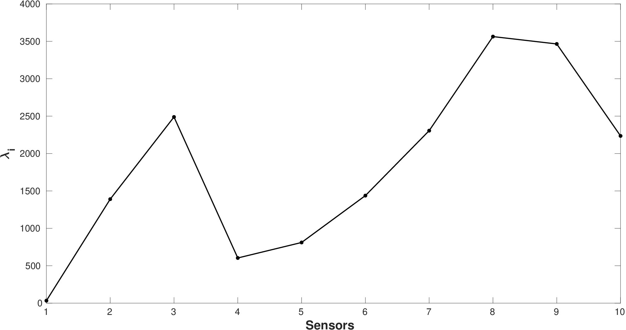
Figure 1: Plot of sensor covariance values for 10 sensors for prescribed lower bound on 𝑷{\color[rgb]{0,0,0}\boldsymbol{P}}. Circle denotes covariance values calculated from minimization of l1l_{1} norm of the vector 𝝀{\color[rgb]{0,0,0}\boldsymbol{\lambda}}

The 𝝀{\color[rgb]{0,0,0}\boldsymbol{\lambda}} vector of sensors for l1l_{1} norm shown in fig(1) are:

𝝀=\displaystyle{\color[rgb]{0,0,0}\boldsymbol{\lambda}}= [33.333 1390.292 2488.968 604.108 811.228\displaystyle[33.333\ 1390.292\ 2488.968\ 604.108\ 811.228
1437.797 2305.879 3563.793 3465.244 2235.787]\displaystyle 1437.797\ 2305.879\ 3563.793\ 3465.244\ 2235.787]

The 𝑹:=diag​(𝝀){\color[rgb]{0,0,0}\boldsymbol{R}}:=\text{diag}({\color[rgb]{0,0,0}\boldsymbol{\lambda}}) noise covariance that we calculated is the minimum noise that needs to be in the measurements to ensure that the steady state error covariance matrix is greater than the prescribed lower bound 𝑷lf{\color[rgb]{0,0,0}\boldsymbol{P}}^{f}_{l}. This is verified by calculating the eigen values of the 𝑷−𝑷lf{\color[rgb]{0,0,0}\boldsymbol{P}}-{\color[rgb]{0,0,0}\boldsymbol{P}}^{f}_{l} matrix, which turns out to be all positive. Matrix 𝑷{\color[rgb]{0,0,0}\boldsymbol{P}} is the DARE solution for the optimal 𝑹{\color[rgb]{0,0,0}\boldsymbol{R}}. We notice that there is a large gap between the lower bound and the final steady state value of 𝑷{\color[rgb]{0,0,0}\boldsymbol{P}}. This is due to the fact that we used eigen value approximations in deriving the result. An ad-hoc method to reduce this gap is to iteratively reduce the magnitude of the 𝝀{\color[rgb]{0,0,0}\boldsymbol{\lambda}} till the eigenvalues of 𝑷−𝑷lf{\color[rgb]{0,0,0}\boldsymbol{P}}-{\color[rgb]{0,0,0}\boldsymbol{P}}^{f}_{l} remain all positive. We found out that we can reduce the 𝝀{\color[rgb]{0,0,0}\boldsymbol{\lambda}} by a factor of 0.080.08 and still ensure 𝑷⪰𝑷lf{\color[rgb]{0,0,0}\boldsymbol{P}}\succeq{\color[rgb]{0,0,0}\boldsymbol{P}}^{f}_{l}.

The calculated 𝑹{\color[rgb]{0,0,0}\boldsymbol{R}} can be assumed to be comprised of actual measurement noise due to the system 𝑹a{\color[rgb]{0,0,0}\boldsymbol{R}}_{a} and synthetic noise 𝑹s{\color[rgb]{0,0,0}\boldsymbol{R}}_{s}. Since in most practical cases 𝑹a{\color[rgb]{0,0,0}\boldsymbol{R}}_{a} is known, our algorithm effectively calculates the minimum synthetic noise 𝑹s{\color[rgb]{0,0,0}\boldsymbol{R}}_{s} that needs to be added to the actual measurement to ensure privacy with respect to state estimation.

8 Conclusion

In this paper we formulate an algorithm to calculate the measurement noise covariance which ensures that the steady state error covariance of the state estimates are lower-bounded by a prescribed bound. We introduce a modified Unified Algebraic Riccati Equation (R-UARE) and exploit eigen value analysis to construct a feasible set of measurement noise covariance. This feasible set is convex and is represented as an LMI. We choose a convex cost function over this convex feasible set of measurement noise covariance, and calculate an optimal noise covariance for system design, which is studied numerically in an example.

References

  • Anderson and Moore (1979) Anderson, B.D. and Moore, J.B. (1979). Optimal filtering. Englewood Cliffs, 21, 22–95.
  • Bryson (2018) Bryson, A.E. (2018). Applied optimal control: optimization, estimation and control. Routledge.
  • Butler et al. (2015) Butler, D.J., Huang, J., Roesner, F., and Cakmak, M. (2015). The privacy-utility tradeoff for remotely teleoperated robots. In Proceedings of the Tenth Annual ACM/IEEE International Conference on Human-Robot Interaction, 27–34. ACM.
  • Dwork et al. (2014) Dwork, C., Roth, A., et al. (2014). The algorithmic foundations of differential privacy. Foundations and Trends® in Theoretical Computer Science, 9(3–4), 211–407.
  • Ghahremani and Kamwa (2011) Ghahremani, E. and Kamwa, I. (2011). Dynamic state estimation in power system by applying the extended kalman filter with unknown inputs to phasor measurements. IEEE Transactions on Power Systems, 26(4), 2556–2566.
  • Kirubarajan and Bar-Shalom (2003) Kirubarajan, T. and Bar-Shalom, Y. (2003). Kalman filter versus imm estimator: when do we need the latter? IEEE Transactions on Aerospace and Electronic Systems, 39(4), 1452–1457. 10.1109/TAES.2003.1261143.
  • Lee (2003) Lee, C.H. (2003). Matrix bounds of the solutions of the continuous and discrete riccati equations–a unified approach. International Journal of Control, 76(6), 635–642.
  • Middleton and Goodwin (1990) Middleton, R.H. and Goodwin, G.C. (1990). Digital Control and Estimation: A Unified Approach (Prentice Hall Information and System Sciences Series). Prentice Hall Englewood Cliffs, NJ.
  • Sima and Benner (2015) Sima, V. and Benner, P. (2015). Solving linear matrix equations with slicot. European Control Conference, ECC 2003.
  • Singh et al. (2017) Singh, P., Chen, M., Carlone, L., Karaman, S., Frazzoli, E., and Hsu, D. (2017). Supermodular mean squared error minimization for sensor scheduling in optimal kalman filtering. In 2017 American Control Conference (ACC), 5787–5794. IEEE.
  • Song et al. (2018) Song, Y., Wang, C.X., and Tay, W.P. (2018). Privacy-aware kalman filtering. In 2018 IEEE International Conference on Acoustics, Speech and Signal Processing (ICASSP). IEEE. 10.1109/icassp.2018.8462600.
  • Tzoumas et al. (2016) Tzoumas, V., Jadbabaie, A., and Pappas, G.J. (2016). Near-optimal sensor scheduling for batch state estimation: Complexity, algorithms, and limits. In 2016 IEEE 55th Conference on Decision and Control (CDC), 2695–2702. IEEE.
  • Work et al. (2008) Work, D.B., Tossavainen, O.P., Blandin, S., Bayen, A.M., Iwuchukwu, T., and Tracton, K. (2008). An ensemble kalman filtering approach to highway traffic estimation using gps enabled mobile devices. In 2008 47th IEEE Conference on Decision and Control, 5062–5068. IEEE.
  • Yi et al. (2013) Yi, T.H., Li, H.N., and Gu, M. (2013). Wavelet based multi-step filtering method for bridge health monitoring using gps and accelerometer. Smart Structures and Systems, 11(4), 331–348.
  • Zhang et al. (2017) Zhang, H., Ayoub, R., and Sundaram, S. (2017). Sensor selection for kalman filtering of linear dynamical systems: Complexity, limitations and greedy algorithms. Automatica, 78, 202–210.