跳到论文正文
W Papers独立论文阅读器 arXiv:2003.05958 论文正文 计算阅读时间 · 0%
引用这篇论文根据当前论文元数据生成,正式投稿前建议核对。


License: arXiv.org perpetual non-exclusive license
arXiv:2003.05958v2 [q-fin.TR] 26 Oct 2020

Optimal market making with persistent order flow

Paul Jusselin Note: paul.jusselin@polytechnique.edu Affiliation: École Polytechnique, CMAP
Abstract

We address the issue of market making on electronic markets when taking into account the clustering and long memory properties of market order flows. We consider a market model with one market maker and order flows driven by general Hawkes processes. We formulate the market maker’s objective as a stochastic control problem. We characterize an optimal control by proving existence and uniqueness of a viscosity solution to the associated Hamilton-Jacobi-Bellman equation. Finally we propose a fully consistent numerical method allowing to implement this optimal strategy in practice.

Keywords: Hawkes processes, market making, high frequency trading, stochastic control, partial differential equations, viscosity solutions.

1 Introduction

Most electronic exchanges are organized as anonymous continuous double auction systems. Market participants can send limit orders to a central limit order book (LOB for short) displaying the volume of shares and the price at which they stand ready to buy or sell those shares. Market participants can also use market orders specifying a volume to buy or sell instantaneously at the best available price. In a very stylized view we can consider that there are two types of market participants: market takers seeking to buy or sell shares for strategic purposes using market orders and market makers filling the LOB with limit orders. Market makers play the role of intermediaries between buyers and sellers market takers.

In practice one of the main risks faced by a market maker is the inventory risk. For example if he has a large positive inventory, price may decrease to his disadvantage. Market makers thus design their strategies in order to mitigate this risk. Basically we expect a market maker with a large positive inventory to set attractive ask prices and less competitive bid prices to attract more buy than sell market orders. More generally he must adapt his strategy to the main statistical features of order flows. Two key stylized facts market makers should take into account in their trading strategies are the clustering and long memory properties of market order flows. The clustering property refers to the fact that buy and sell market orders are not distributed homogeneously in time but tend to be clustered, see [14]. In practice it means that after a buy (for say) market order it is likely that a new one is going to be sent shortly. The long memory of market order flows means the autocorrelation function of trades signs (+1+1 for a buy order and −1-1 for a sell order) has a power-law tail, see [19]. In this paper our goal is to propose a method to design market making strategies that take into account those two features of market order flows.

The issue of market making while managing inventory risk has been notably addressed in [3, 11] where market order flows are modeled using Poisson processes, see also the books [5, 10]. But Poisson processes neither reproduce the clustering nor the long memory property of market order flows. Dealing with the same topic the authors of [6, 27] use a refined model based on Hawkes processes with exponential kernels. The same modeling is also used in [2, 14] to design optimal liquidation strategies. With such kernels Hawkes processes reproduce the clustering property of market order flows but not its long memory. However when the kernel has a power law tail, both properties are reproduced, see [4, 18]. Hence in this paper we extend the works [3, 6, 11] to market order flows driven by Hawkes processes with general kernels.

We now make precise the market model we use. We consider a market with one market maker controlling the best bid and ask prices and with market takers sending only market orders of unit volume. We denote by NtaN^{a}_{t} (resp. NtbN^{b}_{t}) the total number of buy (resp. sell) market orders sent between time 00 and time tt and it=Ntb−Ntai_{t}=N_{t}^{b}-N_{t}^{a} the market maker’s inventory, which is null at time 00. As in [3] the market maker controls the bid and ask spreads, denoted by δa\delta^{a} and δb\delta^{b}. The corresponding best ask and bid prices are P+δaP+\delta^{a} and P−δbP-\delta^{b}, where PP is the fundamental price of the underlying asset. The set of admissible controls is then

𝒜={δ=(δa,δb)∈ℝ+2, s.t. δ is predictable},\mathcal{A}=\{\delta=(\delta^{a},\delta^{b})\in\mathbb{R}_{+}^{2},\text{ s.t. }\delta\text{ is predictable}\},

where predictability is relative to the natural filtration generated by (P,Na,Nb)(P,N^{a},N^{b}), see Section 5.1 for more details. Since market takers are seeking for low transaction costs, their trading intensity is decreasing with the spreads. More precisely we know, from classical financial economics results, see [8, 20, 26], that the average number of trades per unit of time is a decreasing function of the ratio between spread and volatility. To model this we consider that market order intensities are given by

λta,δ=e−kσ​δta​λta,0​ and ​λtb,δ=e−kσ​δtb​λtb,0,\lambda^{a,\delta}_{t}=e^{-\frac{k}{\sigma}\delta^{a}_{t}}\lambda^{a,0}_{t}\text{ and }\lambda^{b,\delta}_{t}=e^{-\frac{k}{\sigma}\delta^{b}_{t}}\lambda^{b,0}_{t},

where kk is a positive constant, σ\sigma the price volatility and

λta,0=Φ⁡(∫0tK⁡(t−s)​d​Nsa),λtb,0=Φ⁡(∫0tK⁡(t−s)​d​Nsb),\lambda^{a,0}_{t}=\Phi\big(\int_{0}^{t}K(t-s)\mathrm{d}N^{a}_{s}\big),~\lambda^{b,0}_{t}=\Phi\big(\int_{0}^{t}K(t-s)\mathrm{d}N^{b}_{s}\big),

where Φ\Phi is a continuous function and KK a completely monotone L1L^{1} function11 1 In this paper we consider complete monotony on ℝ+\mathbb{R}_{+}.. Note that if the spreads are null, the processes NaN^{a} and NbN^{b} are, as intended, generalized Hawkes processes with kernel KK. Regarding the dynamics of PP we assume it is given by

d​Pt=d⁡(t,Pt)​d​t+σ​d​Wt\mathrm{d}P_{t}=d(t,P_{t})\mathrm{d}t+\sigma\mathrm{d}W_{t} (1)

where dd is a Lipschitz function.

Inspired by [3, 6, 11] we consider that the market maker’s problem is equivalent to solve the following stochastic control problem:

supδ∈𝒜​𝔼δ​[G⁡(iT,PT)​e−r​T+∫0Te−r​s​(g⁡(is,Ps)​𝑑s+δsa​d​Nsa+δsb​d​Nsb)],\underset{\delta\in\mathcal{A}}{\sup}~\mathbb{E}^{\delta}\Big[G(i_{T},P_{T})e^{-rT}+\int_{0}^{T}e^{-rs}\big(g(i_{s},P_{s})\mathrm{d}s+\delta^{a}_{s}\mathrm{d}N^{a}_{s}+\delta^{b}_{s}\mathrm{d}N^{b}_{s}\big)\Big], (2)

where rr is a positive constant and gg and GG are two continuous functions with at most quadratic growth. The former represents a continuous reward received by the market maker (besides its P&L) and the latter is a final lump sum payment received at the end of the trading horizon. Typical choices would be G⁡(x,y)=x​yG(x,y)=xy and g⁡(x,y)=−x2g(x,y)=-x^{2}. The notation 𝔼δ\mathbb{E}^{\delta} denotes the expectation under the law corresponding to the control δ\delta (see Section 5.1 for details).

When the order flows are Poisson processes (corresponding to ϕ\phi constant) the process (P,i,Na,Nb)(P,i,N^{a},N^{b}) is Markovian. Hence to solve the market maker’s optimization problem the authors of [3] study the associated Hamilton-Jacobi-Bellman equation (HJB for short). However when NaN^{a} and NbN^{b} are general Hawkes processes (P,i,Na,Nb)(P,i,N^{a},N^{b}) is not Markovian22 2 In the exponential case the process (P,i,Na,Nb,λb,λa)(P,i,N^{a},N^{b},\lambda^{b},\lambda^{a}) is Markovian.. In order to circumvent this issue we need to consider auxiliary state variables enabling us to work in a Markovian setting. More precisely we consider the process XK=(P,i,θK,a,θK,b)X^{K}=(P,i,\theta^{K,a},\theta^{K,b}) where

θtK,a​(u)=∫0tK⁡(u−s)​d​Nsa​ and ​θtK,b​(u)=∫0tK⁡(u−s)​d​Nsb.\theta^{K,a}_{t}(u)=\int_{0}^{t}K(u-s)\mathrm{d}N^{a}_{s}\text{ and }\theta^{K,b}_{t}(u)=\int_{0}^{t}K(u-s)\mathrm{d}N^{b}_{s}.

Note33 3 To define θtK,a\theta^{K,a}_{t} and θtK,b\theta^{K,b}_{t} we consider that KK is extended to ℝ\mathbb{R} with value 00 on ℝ−∗\mathbb{R}_{-}^{*}. that θtK,a\theta^{K,a}_{t} and θtK,b\theta^{K,b}_{t} are random functions from ℝ+\mathbb{R}_{+} into ℝ+\mathbb{R}_{+} and that the process (t,XtK)t≥0(t,X^{K}_{t})_{t\geq 0} is Markovian. Studying the HJB equation associated with this representation, we prove in Section 2 that the stochastic control problem (2) admits a solution of the form δtK,∗=δK​(t,XtK)\delta^{K,*}_{t}=\delta^{K}(t,X^{K}_{t}), where δK\delta^{K} is a feedback control function.

The HJB equation associated with (2) and the representation (t,XtK)t≥0(t,X^{K}_{t})_{t\geq 0} is defined on a subset of an infinite dimensional vector space. So we cannot rely on classical numerical methods to approximate δK\delta^{K}. To tackle this issue we propose the following strategy.

  • 1.

    We show that if (Kn)n≥0(K_{n})_{n\geq 0} converges towards KK in L1L^{1} and uniformly on [0,T][0,T] then (δKn,∗)n≥0(\delta^{K_{n},*})_{n\geq 0} converges almost surely towards δK,∗\delta^{K,*}.

  • 2.

    We show that when K⁡(t)=∑i=1nαi​e−γi​tK(t)=\sum_{i=1}^{n}\alpha_{i}e^{-\gamma_{i}t}, there exists a Markovian representation of the model in dimension 2​n+22n+2. Therefore in this case the feedback control δK\delta^{K} can be approximated numerically.

  • 3.

    Inspired by [1], we prove that for any completely monotone kernel KK in L1L^{1}, we can find a sequence (Kn)n≥0(K_{n})_{n\geq 0}, converging towards KK in L1L^{1} and uniformly on [0,T][0,T], such that for any nn, KnK_{n} is a linear combination of decreasing exponential functions.

Those three points show that if KnK_{n} is close from KK then δKn,∗\delta^{K_{n},*}, which is related to a finite dimensional HJB equation, is good approximation of δK,∗\delta^{K,*}. However when nn is large we cannot rely on finite differences methods to compute the feedback control δKn\delta^{K_{n}} since the dimension of the associated HJB equation is too large. Hence for numerical experiments we use the probabilistic representation of semi-linear partial differential equations (PDEs for short) introduced in [13].

The paper is organized as follows. In Section 2 we prove existence of a solution to Problem (2) based on the study of its associated HJB equation. In Section 3 we explain how to approximate the optimal control obtained in Section 2. Finally in Section 4, we present some numerical experiments. Main proofs are relegated to Section 5.

2 Solving the market maker problem

In this section we prove existence of a solution to Problem (2). First we define an appropriate domain for the process XKX^{K}. Then we show that the HJB equation associated to (2) has a unique viscosity solution with polynomial growth on this domain. Finally we prove existence and characterize an optimal control solving (2).

2.1 Appropriate set for the process XKX^{K}

To study uniqueness of solution to a PDE in the sense of viscosity, it is convenient to work with locally compact domain. We have XK=(P,i,θK,a,θK,b)∈ℝ×ℤ×L1×L1X^{K}=(P,i,\theta^{K,a},\theta^{K,b})\in\mathbb{R}\times\mathbb{Z}\times L^{1}\times L^{1}, but L1L^{1} is not locally compact. Hence we need to make precise the set in which the processes θK,a\theta^{K,a} and θK,b\theta^{K,b} belong. Obviously for j=aj=a or bb we have

θtK,j∈ΘtK={∑i=1nK(⋅−Ti),n∈ℕ,T1≤⋯≤Tn≤t}⊂ΘTK.\theta^{K,j}_{t}\in\Theta_{t}^{K}=\{\sum_{i=1}^{n}K(\cdot-T_{i}),~n\in\mathbb{N},~T_{1}\leq\dots\leq T_{n}\leq t\}\subset\Theta^{K}_{T}.

We naturally endow ΘTK\Theta^{K}_{T} with the L1L^{1} topology and prove in Appendix A that it has the following topological properties.

Lemma 2.1.
  • (i)

    The set ΘTK\Theta^{K}_{T} is a locally compact closed subset of L1L^{1}.

  • (ii)

    For any sequence (sn,θn)n≥0(s_{n},\theta_{n})_{n\geq 0} with values in [0,T]×ΘTK[0,T]\times\Theta^{K}_{T} such that for any nn, θn∈ΘsnK\theta_{n}\in\Theta^{K}_{s_{n}}, if (sn,θn)n≥0(s_{n},\theta_{n})_{n\geq 0} converges towards (s,θ)(s,\theta) then we have θ∈ΘsK\theta\in\Theta_{s}^{K} and θn​(sn)→θ⁡(s)\theta_{n}(s_{n})\rightarrow\theta(s) when n→+∞n\rightarrow+\infty.

  • (iii)

    Moreover if KK is a sum of exponential functions then we have for any l≥0,l\geq 0,

    θn(l)​(T)→θ(l)​(T)​, when ​n→+∞.\theta_{n}^{(l)}(T)\rightarrow\theta^{(l)}(T)\text{, when }n\rightarrow+\infty.

Points (i​i)(ii) and (i​i​i)(iii) are purely technical and are used in Section 3. We now define a locally compact domain for the process XKX^{K}. More precisely for any t∈[0,T]t\in[0,T] we consider

𝒵tK={(i,θa,θb)∈ℤ×ΘtK×ΘtK} and 𝒳tK={(p,i,θa,θb) s.t. p∈ℝ and (i,θa,θb)∈𝒵tK}.\mathcal{Z}^{K}_{t}=\{(i,\theta^{a},\theta^{b})\in\mathbb{Z}\times\Theta^{K}_{t}\times\Theta^{K}_{t}\}\text{ and }\mathcal{X}^{K}_{t}=\{(p,i,\theta^{a},\theta^{b})\text{ s.t. }p\in\mathbb{R}\text{ and }(i,\theta^{a},\theta^{b})\in\mathcal{Z}_{t}^{K}\}.

According to Lemma 2.1 (i)(i) the set 𝒵tK\mathcal{Z}^{K}_{t} (resp. 𝒳tK\mathcal{X}^{K}_{t}) is a locally compact closed subset of ℤ×L1×L1\mathbb{Z}\times L^{1}\times L^{1} (resp. ℝ×ℤ×L1×L1\mathbb{R}\times\mathbb{Z}\times L^{1}\times L^{1}). We also define

ℰK={(t,x)∈[0,T]×𝒳TK s.t x∈𝒳tK},\mathcal{E}^{K}=\{(t,x)\in[0,T]\times\mathcal{X}^{K}_{T}\text{ s.t }x\in\mathcal{X}^{K}_{t}\},

which is a locally compact closed subset of [0,T]×ℝ×ℤ×L1×L1[0,T]\times\mathbb{R}\times\mathbb{Z}\times L^{1}\times L^{1}. Obviously for any t∈[0,T]t\in[0,T] we have (t,XtK)∈ℰK(t,X^{K}_{t})\in\mathcal{E}^{K}. Hence ℰK\mathcal{E}^{K} is the appropriate domain to use the theory of viscosity solutions.

Before going to the next section we give additional definitions that we use later on. For x=(p,i,θa,θb)∈ℝ×ℤ×L1×L1x=(p,i,\theta^{a},\theta^{b})\in\mathbb{R}\times\mathbb{Z}\times L^{1}\times L^{1} we define the norm

‖x‖=p2+i2+‖θa‖12+‖θb‖12.\|x\|=\sqrt{p^{2}+i^{2}+\|\theta^{a}\|^{2}_{1}+\|\theta^{b}\|^{2}_{1}}.

Then for any positive RR the following set is a compact subset of ℰK\mathcal{E}^{K}, as consequence of Lemma 2.1 (i)(i),

ℰRK={(t,x)∈ℰK, s.t. ∥x∥≤R}.\mathcal{E}^{K}_{R}=\{(t,x)\in\mathcal{E}^{K}\text{, s.t. }\|x\|\leq R\}.

Finally in order to lighten the notations from now on when we consider x∈ℰKx\in\mathcal{E}^{K} (resp. x∈𝒳tKx\in\mathcal{X}^{K}_{t}, z∈𝒵tKz\in\mathcal{Z}^{K}_{t}) we implicitly assume that x=(t,p,i,θa,θb)x=(t,p,i,\theta^{a},\theta^{b}) (\big(resp. x=(p,i,θa,θb)x=(p,i,\theta^{a},\theta^{b}), z=(i,θa,θb)z=(i,\theta^{a},\theta^{b}) )\big).

Now that we have defined an adapted domain for PDE analysis we derive in the next section the HJB equation related to the stochastic control problem (2).

2.2 Hamilton-Jacobi-Bellman equation associated to the control problem

We start by rewriting the stochastic control problem (2). We note that up to a ℙδ\mathbb{P}^{\delta}-local martingale the integrals

∫0Tδsa​d​Nsa​ and ​∫0Tδsb​d​Nsb.\int_{0}^{T}\delta^{a}_{s}\mathrm{d}N^{a}_{s}\text{ and }\int_{0}^{T}\delta^{b}_{s}\mathrm{d}N^{b}_{s}.

are respectively equal to ∫0Tδsa​λsa,δ​𝑑s\int_{0}^{T}\delta^{a}_{s}\lambda^{a,\delta}_{s}\mathrm{d}s and ∫0Tδsb​λsb,δ​𝑑s\int_{0}^{T}\delta^{b}_{s}\lambda^{b,\delta}_{s}\mathrm{d}s . Hence as a consequence of Appendix B.3 for any δ∈𝒜\delta\in\mathcal{A} we have

𝔼δ[G(iT,PT)e−r​T+\displaystyle\mathbb{E}^{\delta}[G(i_{T},P_{T})e^{-rT}+ ∫0Te−r​s(g(is,Ps)ds+δsadNsa+δsbdNsb)]\displaystyle\int_{0}^{T}e^{-rs}\Big(g(i_{s},P_{s})\mathrm{d}s+\delta^{a}_{s}\mathrm{d}N^{a}_{s}+\delta^{b}_{s}\mathrm{d}N^{b}_{s}\Big)]
=𝔼δ​[G⁡(iT,PT)​e−r​T+∫0Te−r​s​(g⁡(is,Ps)+δsa​λsa,δ+δsb​λsb,δ)​𝑑s].\displaystyle=\mathbb{E}^{\delta}[G(i_{T},P_{T})e^{-rT}+\int_{0}^{T}e^{-rs}\Big(g(i_{s},P_{s})+\delta^{a}_{s}\lambda^{a,\delta}_{s}+\delta^{b}_{s}\lambda^{b,\delta}_{s}\Big)\mathrm{d}s].

Thus (2) is equivalent to the stochastic control problem

supδ∈𝒜​𝔼δ​[G⁡(iT,PT)​e−r​T+∫0Te−r​s​(g⁡(is,Ps)+δsa​λsa,δ+δsb​λsb,δ)​𝑑s].\underset{\delta\in\mathcal{A}}{\sup}~\mathbb{E}^{\delta}[G(i_{T},P_{T})e^{-rT}+\int_{0}^{T}e^{-rs}\Big(g(i_{s},P_{s})+\delta^{a}_{s}\lambda^{a,\delta}_{s}+\delta^{b}_{s}\lambda^{b,\delta}_{s}\Big)\mathrm{d}s]. (3)

In order to give intuition on the HJB equation related to this stochastic control problem we write the Ito formula related to XKX^{K} for a fixed control δ∈𝒜\delta\in\mathcal{A}. We consider a function φ\varphi defined on [0,T]×ℝ×ℤ×L1×L1[0,T]\times\mathbb{R}\times\mathbb{Z}\times L^{1}\times L^{1} that is C2,2,0,0,0C^{2,2,0,0,0}. We call any function with such regularity a test function. For any s<t∈[0,T]s<t\in[0,T] we have

φ(t,XtK)−φ(s,XsK)=∫st\displaystyle\varphi(t,X^{K}_{t})-\varphi(s,X^{K}_{s})=\int_{s}^{t} (∂tφ⁡(u,Xu−K)+ℒP​φ​(u,Xu−K)+∑j=a,bDjK​φ​(u,Xu−K)​e−kσ​δuj​Φ​(θuK,j​(u)))​d​u\displaystyle\Big(\partial_{t}\varphi(u,X^{K}_{u-})+\mathcal{L}^{P}\varphi(u,X^{K}_{u-})+\sum_{j=a,b}D^{K}_{j}\varphi(u,X^{K}_{u-})e^{-\frac{k}{\sigma}\delta^{j}_{u}}\Phi\big(\theta_{u}^{K,j}(u)\big)\Big)\mathrm{d}u
+∂pφ(u,Xu−K)σdWu+DaKφ(u,Xu−K)dMua;δ+DbKφ(u,Xu−K)dMub;δ,\displaystyle+\partial_{p}\varphi(u,X^{K}_{u-})\sigma\mathrm{d}W_{u}+D^{K}_{a}\varphi(u,X^{K}_{u-})\mathrm{d}M^{a;\delta}_{u}+D^{K}_{b}\varphi(u,X^{K}_{u-})\mathrm{d}M^{b;\delta}_{u},

where

Mta;δ=Nta−∫0tλsa,δ​𝑑s​ and ​Mtb;δ=Ntb−∫0tλsb,δ​𝑑sM^{a;\delta}_{t}=N^{a}_{t}-\int_{0}^{t}\lambda^{a,\delta}_{s}\mathrm{d}s\text{ and }M^{b;\delta}_{t}=N^{b}_{t}-\int_{0}^{t}\lambda^{b,\delta}_{s}\mathrm{d}s

are ℙδ\mathbb{P}^{\delta}-uniformly integrable martingales, see Appendix B.1 for details. The operator ℒP\mathcal{L}^{P} is the infinitesimal generator related to the diffusion of PP and is defined for any test function φ\varphi and (t,x)∈ℰK(t,x)\in\mathcal{E}^{K} by

ℒP​φ​(t,x)=d⁡(t,p)​∂pφ⁡(t,x)+12​σ2​∂p​p2φ⁡(t,x).\mathcal{L}^{P}\varphi(t,x)=d(t,p)\partial_{p}\varphi(t,x)+\frac{1}{2}\sigma^{2}\partial^{2}_{pp}\varphi(t,x).

The operators DaKD^{K}_{a} and DbKD^{K}_{b} correspond to the infinitesimal generators related to the diffusion of NaN^{a} and NbN^{b}. They are defined for (t,x)∈ℰK(t,x)\in\mathcal{E}^{K} by

DaK​φ​(t,x)\displaystyle D^{K}_{a}\varphi(t,x) =φ(t,p,i−1,θa+K(⋅−t),θb)−φ(t,p,i,θa,θb),\displaystyle=\varphi\big(t,p,i-1,\theta^{a}+K(\cdot-t),\theta^{b}\big)-\varphi(t,p,i,\theta^{a},\theta^{b}),
DbK​φ​(t,x)\displaystyle D^{K}_{b}\varphi(t,x) =φ(t,p,i+1,θa,θb+K(⋅−t))−φ(t,p,i,θa,θb).\displaystyle=\varphi\big(t,p,i+1,\theta^{a},\theta^{b}+K(\cdot-t)\big)-\varphi(t,p,i,\theta^{a},\theta^{b}).

Hence the HJB equation associated to the control problem (3) is

(𝐇𝐉𝐁)K:{F⁡(x,U⁡(x),∇U​(x),∂p​p2U⁡(x),DK​U​(x))=0​ for ​x∈ℰK,U⁡(T,y)=G⁡(i,p)​ for ​y∈𝒳TK,(\mathbf{HJB})_{K}:\left\{\begin{array}[]{ll}&F\big(x,U(x),\nabla U(x),\partial^{2}_{pp}U(x),D^{K}U(x)\big)=0\text{ for }x\in\mathcal{E}^{K},\\ &U(T,y)=G(i,p)\text{ for }y\in\mathcal{X}_{T}^{K},\end{array}\right.

with ∇U=(∂tU,∂pU)\nabla U=\big(\partial_{t}U,\partial_{p}U\big), DK​U=(DaK​U,DbK​U)D^{K}U=\big(D^{K}_{a}U,D^{K}_{b}U\big) and where the function FF is defined for (x,u,q,A,I)∈ℰtK×ℝ×ℝ2×ℝ×ℝ2(x,u,q,A,I)\in\mathcal{E}^{K}_{t}\times\mathbb{R}\times\mathbb{R}^{2}\times\mathbb{R}\times\mathbb{R}^{2} by

F⁡(x,u,q,A,I)=\displaystyle F(x,u,q,A,I)= r​u−q1−d⁡(t,p)​q2−12​σ2​A−g⁡(i,p)\displaystyle ru-q_{1}-d(t,p)q_{2}-\frac{1}{2}\sigma^{2}A-g(i,p)
−supδ∈ℝ+​Φ​(θa​(t))​e−kσ​δ​(δ+I1)−supδ∈ℝ+​Φ​(θb​(t))​e−kσ​δ​(δ+I2).\displaystyle-\underset{\delta\in\mathbb{R}_{+}}{\sup}\Phi\big(\theta^{a}(t)\big)e^{-\frac{k}{\sigma}\delta}(\delta+I_{1})-\underset{\delta\in\mathbb{R}_{+}}{\sup}\Phi\big(\theta^{b}(t)\big)e^{-\frac{k}{\sigma}\delta}(\delta+I_{2}).

A straightforward computation gives the maximizers

δ∗a=(σ/k−I1)+​ and ​δ∗b=(σ/k−I2)+.\delta^{*a}=\big(\sigma/k-I_{1}\big)_{+}\text{ and }\delta^{*b}=\big(\sigma/k-I_{2}\big)_{+}. (4)

Note that the dependence in KK of (𝐇𝐉𝐁)K(\mathbf{HJB})_{K} lies in the operator DKD^{K}.

For such general partial-integro differential equation (PIDE for short) it is a priori impossible to prove existence of a smooth solution. Therefore in the next section we look for viscosity solutions.

2.3 Viscosity solutions: definitions

Since we are dealing with a PIDE defined on an unusual domain and in order to make things precise we define the notion of viscosity solution in our framework. First we give the classical definition and then its counterparts based on semi jets.

Definition 2.1.
  • -

    A locally bounded function U∈U​S​C​(ℰK)U\in USC(\mathcal{E}^{K}) (the set of upper semi-continuous functions on ℰK\mathcal{E}^{K}) is a viscosity sub-solution of (𝐇𝐉𝐁)K(\mathbf{HJB})_{K} if for all x∈ℰKx\in\mathcal{E}^{K} and test function ϕ\phi such that xx is a maximum of U−ϕU-\phi we have

    F⁡(x,ϕ⁡(x),∇ϕ​(x),∂p​p2ϕ⁡(x),DK​U​(x))≤0.F\big(x,\phi(x),\nabla\phi(x),\partial^{2}_{pp}\phi(x),D^{K}U(x)\big)\leq 0.
  • -

    A locally bounded function U∈L​S​C​(ℰK)U\in LSC(\mathcal{E}^{K}) (the set of lower semi-continuous functions on ℰK\mathcal{E}^{K}) is a viscosity super-solution of (𝐇𝐉𝐁)K(\mathbf{HJB})_{K} if for all x∈ℰKx\in\mathcal{E}^{K} and test function ϕ\phi such that xx is a minimum of U−ϕU-\phi we have

    F⁡(x,ϕ⁡(x),∇ϕ​(x),∂p​p2ϕ⁡(x),DK​U​(x))≥0.F\big(x,\phi(x),\nabla\phi(x),\partial^{2}_{pp}\phi(x),D^{K}U(x)\big)\geq 0.
  • -

    A continuous function UU defined on ℰK\mathcal{E}^{K} is a viscosity solution of (𝐇𝐉𝐁)K(\mathbf{HJB})_{K} if it is a viscosity super-solution and a viscosity sub-solution.

Note that in the above definition it is equivalent to consider local (or local strict) extrema. Also note that we have not replaced UU by ϕ\phi for the last operator DKD^{K}. This is because DK​UD^{K}U only requires finiteness of UU to be defined. Of course it is equivalent to replace DK​UD^{K}U by DK​ϕD^{K}\phi in Definition 2.1. Indeed consider a sub-solution UU and a test function ϕ\phi at point xx. Since DKD^{K} is a non local operator we can always build a sequence of test functions (ϕn)n≥0(\phi_{n})_{n\geq 0} satisfying U≤ϕnU\leq\phi_{n} with equality at point xx and such that

(∇ϕn​(x),∂p​p2ϕn​(x))=(∇ϕ​(x),∂p​p2ϕ⁡(x))​ with ​DK​ϕn​(x)​→n→+∞​DK​U​(x).(\nabla\phi_{n}(x),\partial^{2}_{pp}\phi_{n}(x))=(\nabla\phi(x),\partial^{2}_{pp}\phi(x))\text{ with }D^{K}\phi_{n}(x)\underset{n\rightarrow+\infty}{\rightarrow}D^{K}U(x).

By continuity of FF we get the equivalence. This also holds for super-solution.

We now introduce the notions of semi super and sub-jets in our framework. For UU in U​S​C​(ℰK)USC(\mathcal{E}^{K}) and x=(t,p,z)∈ℰKx=(t,p,z)\in\mathcal{E}^{K}, the super-jet of UU at point xx is the set

𝒥+​U​(x)=\displaystyle\mathcal{J}^{+}U(x)= {(g,A,h)∈ℝ2×ℝ×C0(𝒵TK), s.t. for any y=(s,q,v)∈ℰK we have\displaystyle\{(g,A,h)\in\mathbb{R}^{2}\times\mathbb{R}\times C^{0}(\mathcal{Z}^{K}_{T}),\text{ s.t. for any }y=(s,q,v)\in\mathcal{E}^{K}\text{ we have }
U⁡(s,y)≤U⁡(t,x)+g1​(t−s)+g2​(p−q)+12​A​(p−q)2+h⁡(z−v)+o⁡(|t−s|+|p−q|2)\displaystyle~U(s,y)\leq U(t,x)+g_{1}(t-s)+g_{2}(p-q)+\frac{1}{2}A(p-q)^{2}+h(z-v)+o(|t-s|+|p-q|^{2})
and h(0)=0}\displaystyle~\text{and }h(0)=0\}

and the semi super-jet of UU at point xx is

𝒥¯+​U​(x)=\displaystyle\overline{\mathcal{J}}^{+}U(x)= {(g,A,h)∈ℝ2×ℝ×C0(𝒵TK) s.t. there exists a sequence\displaystyle\{(g,A,h)\in\mathbb{R}^{2}\times\mathbb{R}\times C^{0}(\mathcal{Z}^{K}_{T})\text{ s.t. there exists a sequence}
(xn,gn,An,hn)n≥0​ with for any ​n≥0​(gn,An,hn)∈𝒥+​U​(xn)\displaystyle~(x_{n},g_{n},A_{n},h_{n})_{n\geq 0}\text{ with for any }n\geq 0~(g_{n},A_{n},h_{n})\in\mathcal{J}^{+}U(x_{n})
 and such that(xn,U(xn),gn,An,hn)→n→+∞(x,U(x),g,A,h)}.\displaystyle~\text{ and such that}\big(x_{n},U(x_{n}),g_{n},A_{n},h_{n}\big)\underset{n\rightarrow+\infty}{\rightarrow}\big(x,U(x),g,A,h\big)\}.

In the above definition the convergence of hnh_{n} is taken in the sense of locally uniform convergence at point 00. By analogy we define the sub-jet 𝒥−​U​(x)\mathcal{J}^{-}U(x) and the semi sub-jet 𝒥¯−​U​(x)\overline{\mathcal{J}}^{-}U(x) for UU in L​S​C​(ℰK)LSC(\mathcal{E}^{K}).

We can now give another characterization of viscosity sub and super-solutions relying on the notions of semi jets.

Definition 2.2.
  • -

    A locally bounded function U∈U​S​C​(ℰK)U\in USC(\mathcal{E}^{K}) is a viscosity sub-solution of (𝐇𝐉𝐁)K(\mathbf{HJB})_{K} if for all x∈ℰKx\in\mathcal{E}^{K}, and (g,A,h)∈𝒥¯+​U​(x)(g,A,h)\in\overline{\mathcal{J}}^{+}U(x) we have

    F⁡(x,U⁡(x),g,A,DK​U​(x))≤0.F\big(x,U(x),g,A,D^{K}U(x)\big)\leq 0.
  • -

    A locally bounded function U∈L​S​C​(ℰK)U\in LSC(\mathcal{E}^{K}) is a viscosity super-solution of (𝐇𝐉𝐁)K(\mathbf{HJB})_{K} if for all x∈ℰKx\in\mathcal{E}^{K}, and (g,A,h)∈𝒥¯−​U​(x)(g,A,h)\in\overline{\mathcal{J}}^{-}U(x) we have

    F⁡(x,U⁡(x),g,A,DK​U​(x))≥0.F\big(x,U(x),g,A,D^{K}U(x)\big)\geq 0.

We show in Appendix C that Definition 2.1 and 2.2 are equivalent.

In the next section based on the study of (𝐇𝐉𝐁)K(\mathbf{HJB})_{K} we prove that the control problem (2) admits a solution.

2.4 Existence of an optimal control

In this section we prove existence of a solution to Problem (3), which is equivalent to (2). Before stating the result we give a sketch of the proof.

We start by proving uniqueness of a viscosity solution with polynomial growth to (𝐇𝐉𝐁)K(\mathbf{HJB})_{K} using a comparison result. The main difficulty is to adapt the Crandall-Ishi’s lemma to our framework, which is done in Appendix D. Using a verification argument we then check that the continuation utility function UKU^{K} associated to Problem (3) is actually this unique solution. The maximizers of the Hamiltonian given in Equation (4) then naturally provide a control solving (3) and therefore Problem (2). Full proof is given in Section 5.2.

Theorem 2.1.
  • (i)

    There exists a unique viscosity solution UKU^{K} with polynomial growth to (𝐇𝐉𝐁)K(\mathbf{HJB})_{K}.

  • (ii)

    This solution satisfies:

    UK​(0)=supδ∈𝒜​𝔼δ​[G⁡(iT,PT)​e−r​T+∫0Te−r​s​(g⁡(is,Ps)+δsa​λsa,δ+δsb​λsb,δ)​𝑑s].U^{K}(0)=\underset{\delta\in\mathcal{A}}{\sup}~\mathbb{E}^{\delta}[G(i_{T},P_{T})e^{-rT}+\int_{0}^{T}e^{-rs}\Big(g(i_{s},P_{s})+\delta^{a}_{s}\lambda^{a,\delta}_{s}+\delta^{b}_{s}\lambda^{b,\delta}_{s}\Big)\mathrm{d}s].
  • (iii)

    Problem (2) admits a solution given by

    δtK,∗=δK​(t,XtK), with ​δK=(δaK,δbK),\delta^{K,*}_{t}=\delta^{K}(t,X^{K}_{t}),\text{ with }\delta^{K}=(\delta^{K}_{a},\delta^{K}_{b}),

    where

    δaK=(σ/k−DaK​UK)+​ and ​δbK=(σ/k−DbK​UK)+.\delta_{a}^{K}=\big(\sigma/k-D^{K}_{a}U^{K}\big)_{+}\text{ and }\delta_{b}^{K}=\big(\sigma/k-D^{K}_{b}U^{K}\big)_{+}. (5)

It is important to note that in order to obtain existence of an admissible optimal control we have benefited from the fact that we are dealing with counting processes, whose infinitesimal generators are defined for any finite functions independently of their regularity. From a practical point of view Theorem 2.1 implies that if we manage to compute UKU^{K} we can implement the optimal control δK,∗\delta^{K,*} by monitoring the processes θa\theta^{a} and θb\theta^{b}. Note that this is equivalent to monitor the list of arrival times of buy and sell market orders. However ℰK\mathcal{E}^{K} is a subset of an infinite dimensional vector space. So we cannot compute UKU^{K} using classic numerical methods. Therefore we need to find another way to approximate the control δK,∗\delta^{K,*}. We deal with this issue in the next section.

3 How to approximate the optimal control

In this section we explain how to approximate numerically the feedback control δK,∗\delta^{K,*}. We proceed in three steps:

  • 1.

    We show that if (Kn)n≥0(K_{n})_{n\geq 0} converges towards KK in L1L^{1} and uniformly on [0,T][0,T] then (δKn,∗)n≥0(\delta^{K_{n},*})_{n\geq 0} converges almost surely towards δK,∗\delta^{K,*}.

  • 2.

    We prove that when K⁡(t)=∑i=1𝑛​αi​e−γi​tK(t)=\overset{n}{\underset{i=1}{\sum}}\alpha_{i}e^{-\gamma_{i}t} there exists a Markovian representation of the model in dimension 2​n+22n+2.

  • 3.

    Inspired by [1], we show that for any completely monotone function KK in L1L^{1} we can find a sequence (Kn)n≥0(K_{n})_{n\geq 0} converging towards KK in L1L^{1} and uniformly on [0,T][0,T] such that for any nn, KnK_{n} is a linear combination of nn decreasing exponential functions.

Those three points give a simple method to compute an approximate version of the control δK,∗\delta^{K,*}: choose K~\tilde{K}, a sum of decreasing exponential functions, close enough to KK. Use the finite dimensional representation to compute UK~U^{\tilde{K}} and implement δK~,∗\delta^{\tilde{K},*} instead of δK,∗\delta^{K,*}.

3.1 Convergence of solutions and optimal controls

Consider a completely monotone function KK in L1L^{1}. We show that if a sequence of continuous L1L^{1} functions (Kn)n≥0(K_{n})_{n\geq 0} converges towards KK in L1L^{1} and uniformly on [0,T][0,T] then the sequence (δKn,∗)n≥0(\delta^{K_{n},*})_{n\geq 0} converges almost surely towards δK,∗\delta^{K,*}.

From Theorem 5.8 in [25] we observe that the notion of viscosity solution is perfectly adapted to prove the convergence of solutions to a sequence of PIDEs. Hence we prove in Section 5.3 the following result which is an extension of Theorem 5.8 in [25] to our framework.

Proposition 3.1.

Consider a sequence (Kn)n≥0(K_{n})_{n\geq 0} of continuous L1L^{1} functions converging towards a completely monotone function KK in L1L^{1} and uniformly on [0,T][0,T], then for any x∈ℰKx\in\mathcal{E}^{K} we have

UK​(x)=lim(y,n)∈ℰ¯→(x,+∞)∈ℰ¯​UKn​(y)U^{K}(x)~=\underset{(y,n)\in\bar{\mathcal{E}}\rightarrow(x,+\infty)\in\bar{\mathcal{E}}}{\lim}~U^{K_{n}}(y) (6)

where

ℰ¯=(⋃n≥0ℰKn×{n})∪(ℰK×{+∞}).\bar{\mathcal{E}}=\big(\bigcup_{n\geq 0}\mathcal{E}^{K_{n}}\times\{n\}\big)\cup\big(\mathcal{E}^{K}\times\{+\infty\}\big).

The main technical difficulty in the proof of Proposition 3.1, compared to Theorem 5.8 in [25], is that the functions (UKn)n≥0(U^{K_{n}})_{n\geq 0} are defined on different domains.

We now consider a fixed sequence (Kn)n≥0(K_{n})_{n\geq 0} of continuous L1L^{1} functions converging towards KK in L1L^{1} and uniformly on [0,T][0,T]. We have that almost surely

((t,XtKn),n)∈ℰ¯→((t,XtK),+∞)∈ℰ¯​ when ​n→+∞.\big((t,X^{K_{n}}_{t}),n\big)\in\bar{\mathcal{E}}\rightarrow\big((t,X^{K}_{t}),+\infty\big)\in\bar{\mathcal{E}}\text{ when }n\rightarrow+\infty.

From now on, when we consider a similar limit result we forget to write ℰ¯\bar{\mathcal{E}} to lighten notations.

We first recall that δtK,∗=(δtK,a,∗,δtK,b,∗)\delta^{K,*}_{t}=(\delta^{K,a,*}_{t},\delta^{K,b,*}_{t}) with

δtK,a,∗\displaystyle\delta^{K,a,*}_{t} =DaK​UK​(t,XtK)=UK​(t,XtK,+a)−UK​(t,XtK),\displaystyle=D^{K}_{a}U^{K}(t,X^{K}_{t})=U^{K}(t,X^{K,+a}_{t})-U^{K}(t,X^{K}_{t}),
δtK,b,∗\displaystyle\delta^{K,b,*}_{t} =DbK​UK​(t,XtK)=UK​(t,XtK,+b)−UK​(t,XtK).\displaystyle=D^{K}_{b}U^{K}(t,X^{K}_{t})=U^{K}(t,X^{K,+b}_{t})-U^{K}(t,X^{K}_{t}).

where

XtK,+a=(Pt,i+1,θtK,a+K(⋅−t),θtK,b) and XtK,+b=(Pt,i+1,θtK,a,θtK,b+K(⋅−t)).X^{K,+a}_{t}=\big(P_{t},i+1,\theta^{K,a}_{t}+K(\cdot-t),\theta^{K,b}_{t}\big)\text{ and }X^{K,+b}_{t}=\big(P_{t},i+1,\theta^{K,a}_{t},\theta^{K,b}_{t}+K(\cdot-t)\big).

Obviously we have the following almost sure convergences

((t,XtKn,+a),n)​→n→+∞​((t,XtK,+a),+∞)​ and ​((t,XtKn,+b),n)​→n→+∞​((t,XtK,+b),+∞).\big((t,X^{K_{n},+a}_{t}),n\big)\underset{n\rightarrow+\infty}{\rightarrow}\big((t,X^{K,+a}_{t}),+\infty\big)\text{ and }\big((t,X^{K_{n},+b}_{t}),n\big)\underset{n\rightarrow+\infty}{\rightarrow}\big((t,X^{K,+b}_{t}),+\infty\big).

So according to Proposition 3.1 we get that almost surely

(UKn​(t,XtKn),UKn​(t,XtKn,+a),UKn​(t,XtKn,+b))​→n→+∞​(UK​(t,XtK),UK​(t,XtK,+a),UK​(t,XtK,+b)).\big(U^{K_{n}}(t,X^{K_{n}}_{t}),U^{K_{n}}(t,X^{K_{n},+a}_{t}),U^{K_{n}}(t,X^{K_{n},+b}_{t})\big)\underset{n\rightarrow+\infty}{\rightarrow}\big(U^{K}(t,X^{K}_{t}),U^{K}(t,X^{K,+a}_{t}),U^{K}(t,X^{K,+b}_{t})\big).

Hence we obtain the following result.

Proposition 3.2.

Consider a sequence (Kn)n≥0(K_{n})_{n\geq 0} of continuous L1L^{1} functions converging towards a completely monotone function KK in L1L^{1} and uniformly on [0,T][0,T], then for any tt we have almost surely

limn→+∞δtKn,∗=δtK,∗.\lim\limits_{n\rightarrow+\infty}\delta^{K_{n},*}_{t}=\delta^{K,*}_{t}.

Proposition 3.2 perfectly fits our purpose of approximating δK,∗\delta^{K,*}. Indeed suppose we manage to find a dense44 4 Here dense is intended in the sense of convergence in L1L^{1}, together with uniform convergence on [0,T][0,T]. subset of the completely monotone L1L^{1} functions such that for any K′K^{\prime} in this subset, the control δK′,∗\delta^{K^{\prime},*} can be approximated numerically. Then Propositions 3.1 and 3.2 guarantee that for any completely monotone function KK in L1L^{1} we can approximate numerically UKU^{K} and δK,∗\delta^{K,*}.

We show in the next two sections that the set

𝒮ℰ=⋃n≥0{∑i=1nαie−γi⋅𝟏ℝ+ s.t. α∈ℝ+n and γ∈ℝ+n}\mathcal{SE}=\bigcup_{n\geq 0}\{\sum_{i=1}^{n}\alpha_{i}e^{-\gamma_{i}\cdot}\mathbf{1}_{\mathbb{R}_{+}}\text{ s.t. }\alpha\in\mathbb{R}_{+}^{n}\text{ and }\gamma\in\mathbb{R}_{+}^{n}\}

satisfies those two conditions. Note that 𝒮​ℰ\mathcal{SE} is simply the set of positive linear combinations of decreasing exponential functions. In the next two sections we study Problem (3) when the function KK is in 𝒮​ℰ\mathcal{SE} and then show that 𝒮​ℰ\mathcal{SE} is dense in the set of completely monotone functions in L1L^{1}.

3.2 Solving the market maker’s problem when K∈𝒮​ℰK\in\mathcal{SE}

In this section we explain how to solve Problem (3) when the kernel function KK is in 𝒮​ℰ\mathcal{SE}.

We consider that the kernel of the Hawkes processes NaN^{a} and NbN^{b} is

Kα,γ​(t)=∑i=1nαi​e−γi​t​𝟏ℝ+​(t),K_{\alpha,\gamma}(t)=\sum_{i=1}^{n}\alpha_{i}e^{-\gamma_{i}t}\mathbf{1}_{\mathbb{R}_{+}}(t),

where nn is a positive integer, α∈ℝ+n\alpha\in\mathbb{R}_{+}^{n} and γ∈ℝ+n\gamma\in\mathbb{R}^{n}_{+}. For i∈{1,…,n}i\in\{1,\dots,n\} and j=aj=a or bb we define the process

ctj,i=∫0tαi​e−γi​(t−s)​d​Nsj.c^{j,i}_{t}=\int_{0}^{t}\alpha_{i}e^{-\gamma_{i}(t-s)}\mathrm{d}N^{j}_{s}.

Then Ytα,γ=(t,Pt,it,(cta,i)1≤i≤n,(ctb,i)1≤i≤n)Y^{\alpha,\gamma}_{t}=\big(t,P_{t},i_{t},(c_{t}^{a,i})_{1\leq i\leq n},(c_{t}^{b,i})_{1\leq i\leq n}\big) is a Markovian process since for j=aj=a or bb

λtj,0=Φ⁡(∑i=1nctj,i)​ and ​d​ctj,i=−γi​ctj,i​d​t+αi​d​Ntj.\lambda^{j,0}_{t}=\Phi(\sum_{i=1}^{n}c^{j,i}_{t})\text{ and }\mathrm{d}c^{j,i}_{t}=-\gamma_{i}c^{j,i}_{t}\mathrm{d}t+\alpha_{i}\mathrm{d}N^{j}_{t}.

The domain associated with this representation is ℰn=[0,T]×ℝ×ℤ×ℝ+n×ℝ+n\mathcal{E}^{n}=[0,T]\times\mathbb{R}\times\mathbb{Z}\times\mathbb{R}_{+}^{n}\times\mathbb{R}_{+}^{n}, which is locally compact. As for ℰK\mathcal{E}^{K}, when we have (t,x)∈ℰn(t,x)\in\mathcal{E}^{n} we implicitly consider that x=(p,i,ca,cb)x=(p,i,c^{a},c^{b}). Note that we can naturally go from the first representation to this one. More precisely we prove in Appendix E that there exists a continuous function Rα,γR^{\alpha,\gamma} from ℰKα,γ\mathcal{E}^{K_{\alpha,\gamma}} into ℰn\mathcal{E}^{n} such that for any t>0t>0 we have Rα,γ​(t,XtKα,γ)=(t,Ytα,γ)R^{\alpha,\gamma}(t,X^{K_{\alpha,\gamma}}_{t})=(t,Y^{\alpha,\gamma}_{t}). However notice that the second representation is somehow larger than the first one.

The infinitesimal generators associated to the processes NaN^{a} and NbN^{b} for the new representation are denoted by DaαD^{\alpha}_{a} and DbαD^{\alpha}_{b}. They are defined for any function UU on ℰn\mathcal{E}^{n} and x∈ℰnx\in\mathcal{E}^{n} by

Daα​U​(x)\displaystyle D_{a}^{\alpha}U(x) =U⁡(t,p,i−1,ca+α,cb)−U⁡(t,p,i,ca,cb),\displaystyle=U(t,p,i-1,c^{a}+\alpha,c^{b})-U(t,p,i,c^{a},c^{b}),
Dbα​U​(x)\displaystyle D_{b}^{\alpha}U(x) =U⁡(t,p,i+1,ca,cb+α)−U⁡(t,p,i,ca,cb).\displaystyle=U(t,p,i+1,c^{a},c^{b}+\alpha)-U(t,p,i,c^{a},c^{b}).

The HJB equation related to Problem (3) in this new representation is therefore

(𝐇𝐉𝐁)α,γ:{Gα,γ(x,U(x),∇cU(x),∇U(x),∂2p​pU(x),DαU(x))=0, for x∈ℰn,U⁡(T,y)=G⁡(i,p)​ for ​(T,y)∈ℰn(\mathbf{HJB})_{\alpha,\gamma}:~\left\{\begin{array}[]{ll}&G_{\alpha,\gamma}\big(x,U(x),\nabla^{c}U(x),\nabla U(x),\partial^{2}_{pp}U(x),D^{\alpha}U(x)\big)=0,\text{ for }x\in\mathcal{E}^{n},\\ &U(T,y)=G(i,p)\text{ for }(T,y)\in\mathcal{E}^{n}\end{array}\right.

with ∇cU=(∇acU,∇bcU)\nabla^{c}U=(\nabla^{c}_{a}U,\nabla^{c}_{b}U) where for j=aj=a or bb, ∇jcU=(∂cj,iU)1≤i≤n\nabla^{c}_{j}U=(\partial_{c^{j,i}}U)_{1\leq i\leq n}, ∇U​(t,x)=(∂tU⁡(t,x),∂pU⁡(t,x))\nabla U(t,x)=\big(\partial_{t}U(t,x),\partial_{p}U(t,x)\big),

Dα​U​(t,x)=(Daα​U​(t,x),Dbα​U​(t,x))D^{\alpha}U(t,x)=\big(D^{\alpha}_{a}U(t,x),D^{\alpha}_{b}U(t,x)\big)

and where the function Gα,γG_{\alpha,\gamma} is defined for (x,u,h,q,A,I)∈ℰn×ℝ×(ℝn)2×ℝ2×ℝ×ℝ2(x,u,h,q,A,I)\in\mathcal{E}^{n}\times\mathbb{R}\times(\mathbb{R}^{n})^{2}\times\mathbb{R}^{2}\times\mathbb{R}\times\mathbb{R}^{2} by

Gα,γ​(x,u,q,h,A,I)=\displaystyle G_{\alpha,\gamma}\big(x,u,q,h,A,I\big)= r​u−h1−d⁡(t,p)​h2−12​σ2​A−⟨γ,q1⟩−⟨γ,q2⟩−g⁡(i,p)\displaystyle~ru-h_{1}-d(t,p)h_{2}-\frac{1}{2}\sigma^{2}A-\langle\gamma,q_{1}\rangle-\langle\gamma,q_{2}\rangle-g(i,p)
−supδ∈ℝ+​Φ​(∑i=1nca,i)​e−kσ​δ​(δ+I1)−supδ∈ℝ+​Φ​(∑i=1ncb,i)​e−kσ​δ​(δ+I2).\displaystyle-\underset{\delta\in\mathbb{R}_{+}}{\sup}\Phi(\sum_{i=1}^{n}c^{a,i})e^{-\frac{k}{\sigma}\delta}(\delta+I_{1})-\underset{\delta\in\mathbb{R}_{+}}{\sup}\Phi(\sum_{i=1}^{n}c^{b,i})e^{-\frac{k}{\sigma}\delta}(\delta+I_{2}).

We easily adapt the proof of Theorem 2.1 to (𝐇𝐉𝐁)α,γ(\mathbf{HJB})_{\alpha,\gamma} and prove the following result.

Theorem 3.1.
  • (i)

    There exists a unique continuous viscosity solution with polynomial growth Uα,γU^{\alpha,\gamma} to (𝐇𝐉𝐁)α,γ(\mathbf{HJB})_{\alpha,\gamma}.

  • (ii)

    The solution Uα,γU^{\alpha,\gamma} satisfies

    Uα,γ​(0)=supδ∈𝒜​𝔼δ​[G⁡(iT,PT)​e−r​T+∫0Te−r​s​(g⁡(is,Ps)+δsa​λsa,δ+δsb​λsb,δ)​𝑑s].U^{\alpha,\gamma}(0)=\underset{\delta\in\mathcal{A}}{\sup}~\mathbb{E}^{\delta}[G(i_{T},P_{T})e^{-rT}+\int_{0}^{T}e^{-rs}\big(g(i_{s},P_{s})+\delta^{a}_{s}\lambda^{a,\delta}_{s}+\delta^{b}_{s}\lambda^{b,\delta}_{s}\big)\mathrm{d}s].
  • (iii)

    The stochastic control problem (3) admits a solution δtα,γ,∗\delta^{\alpha,\gamma,*}_{t} satisfying

    δtα,γ,∗=δα,γ​(t,Ytα,γ), with ​δα,γ=(δaδ,γ,δaδ,γ)\delta^{\alpha,\gamma,*}_{t}=\delta^{\alpha,\gamma}(t,Y^{\alpha,\gamma}_{t}),\text{ with }\delta^{\alpha,\gamma}=(\delta^{\delta,\gamma}_{a},\delta^{\delta,\gamma}_{a})

    where

    δaα,γ=(σ/k−Daα​Uα,γ)+​ and ​δbα,γ=(σ/k−Dbα​Uα,γ)+.\delta_{a}^{\alpha,\gamma}=\big(\sigma/k-D^{\alpha}_{a}U^{\alpha,\gamma}\big)_{+}\text{ and }\delta_{b}^{\alpha,\gamma}=\big(\sigma/k-D^{\alpha}_{b}U^{\alpha,\gamma}\big)_{+}.
  • (iv)

    We have UKα,γ=Uα,γ∘ℛα,γU^{K_{\alpha,\gamma}}=U^{\alpha,\gamma}\circ\mathcal{R}^{\alpha,\gamma}.

The proof of the three first points is exactly the same as the proof of Theorem 2.1. We deal with point (i​v)(iv) in Section 5.4. Points (i​i​i)(iii) and (i​v)(iv) of Theorem 3.1 imply that for any α\alpha and γ\gamma in ℝ+n\mathbb{R}_{+}^{n} we can approximate numerically δKα,γ\delta^{K_{\alpha,\gamma}}. We just need to approximate Uα,γU^{\alpha,\gamma} using any numerical method, which is possible because the domain of (𝐇𝐉𝐁)α,γ(\mathbf{HJB})_{\alpha,\gamma} is a subset of a finite dimensional vector space. Then using the change of variable ℛα,γ\mathcal{R}^{\alpha,\gamma} one gets

δKα,γ=δα,γ∘ℛα,γ.\delta^{K_{\alpha,\gamma}}=\delta^{\alpha,\gamma}\circ\mathcal{R}^{\alpha,\gamma}.

Note that this shows that the controls δKα,γ,∗\delta^{K_{\alpha,\gamma},*} given in Theorem 2.1 (iii) and δα,γ,∗\delta^{\alpha,\gamma,*} given in Theorem 3.1 (iii) are actually the same.

3.3 Density of 𝒮​ℰ\mathcal{SE} in the set of completely monotone functions

In this section we show that 𝒮​ℰ\mathcal{SE} is dense in the set of completely monotone functions in L1L^{1}. Before giving the result we present a short sketch of the proof.

The key idea is that any completely monotone function can be written as the Laplace transform of a positive measure mm, see Lemma 2.3 in [21]:

K⁡(x)=∫0+∞e−u​x​m​(𝑑u).K(x)=\int_{0}^{+\infty}e^{-ux}m(\mathrm{d}u). (7)

Moreover if K⁡(0)<+∞K(0)<+\infty then mm is L1L^{1} and if KK is in L1L^{1} then ∫0+∞m⁡(d​u)u<∞\int_{0}^{+\infty}\frac{m(\mathrm{d}u)}{u}<\infty. Hence using Riemann sums to approximate the integral (7) we get a natural way of approximating KK by a sequence of functions in 𝒮​ℰ\mathcal{SE}. Based on this idea we prove the following result in Appendix F.

Lemma 3.1.

For any completely monotone function KK in L1L^{1} there exists a sequence (αn,γn)n≥0(\alpha_{n},\gamma_{n})_{n\geq 0}, such that:

  • (i)(i)

    For any nn, (αn,γn)∈ℝ+n×ℝ+n(\alpha_{n},\gamma_{n})\in\mathbb{R}^{n}_{+}\times\mathbb{R}^{n}_{+},

  • (i​i)(ii)

    (Kαn,γn)n≥0(K_{\alpha_{n},\gamma_{n}})_{n\geq 0} converges towards KK in L1L^{1} and uniformly on every compact set of ℝ+\mathbb{R}_{+},

  • (i​i​i)(iii)

    ‖Kαn,γn‖1=‖K‖1​ and ​Kαn,γn​(0)=K⁡(0).\|K_{\alpha_{n},\gamma_{n}}\|_{1}=\|K\|_{1}\text{ and }K_{\alpha_{n},\gamma_{n}}(0)=K(0).

Lemma 3.1 together with Proposition 3.2 and Theorem 3.1 allows us to conclude on the existence of a procedure to approximate δK,∗\delta^{K,*}. In the next section we sum up our results and explain how to use them in practice.

3.4 Conclusion on approximating the optimal control

For a completely monotone function KK in L1L^{1} consider (αn,γn)n≥0(\alpha_{n},\gamma_{n})_{n\geq 0} a sequence given by Lemma 3.1. We write KnK_{n} instead of Kαn,γnK_{\alpha_{n},\gamma_{n}} to lighten notations. According to Proposition 3.2, we have the following almost sure convergence for any tt

δαn,γn​(t,Ytαn,γn)​→n→+∞​δtK,∗.\delta^{\alpha_{n},\gamma_{n}}(t,Y^{\alpha_{n},\gamma_{n}}_{t})\underset{n\rightarrow+\infty}{\rightarrow}\delta_{t}^{K,*}.

Hence to implement an approximated version of the optimal control δK,∗\delta^{K,*} we simply have to implement the control δtαn,γn,∗\delta^{\alpha_{n},\gamma_{n},*}_{t} for nn large enough. This approximated control can be computed by solving numerically the finite dimensional PIDE (𝐇𝐉𝐁)α,β(\mathbf{HJB})_{\alpha,\beta}.

In conclusion the recipee to implement an approximated version of the optimal control δK,∗\delta^{K,*} is the following:

  • 1.

    Fix nn positive and find α,γ∈ℝ+n\alpha,\gamma\in\mathbb{R}_{+}^{n} such that Kα,γK_{\alpha,\gamma} is the closest possible from KK. See Appendix F for a method to choose such α\alpha and γ\gamma.

  • 2.

    Approximate numerically Uα,γU^{\alpha,\gamma}, the solution of (𝐇𝐉𝐁)α,γ(\mathbf{HJB})_{\alpha,\gamma}, which is equivalent to approximate numerically the feedback δα,γ\delta^{\alpha,\gamma}.

  • 3.

    Monitor Yα,γY^{\alpha,\gamma} and apply the control δα,γ​(t,Yα,γ)\delta^{\alpha,\gamma}(t,Y^{\alpha,\gamma}).

The only flaw of this method is that the set ℰn\mathcal{E}^{n} is a subset of a vector space of dimension 2​n+22n+2. Hence when nn is larger than 22 it is very unlikely that simple finite differences methods can be used to solve numerically (𝐇𝐉𝐁)α,γ(\mathbf{HJB})_{\alpha,\gamma}. To tackle this issue we need to use other numerical methods such as neural networks, see [15] for example, or probabilistic method, see [13]. In this article we propose to use the later method for numerical applications.

4 Numerical applications

In this section we present some numerical experiments illustrating our results. We consider a simplified version of the market maker’s problem:

(N):supδ∈𝒜​𝔼δ​[∫0Tδsa​d​Nsa+δsb​d​Nsb−μ​is2​𝑑s].(N):\underset{\delta\in\mathcal{A}}{\sup}~\mathbb{E}^{\delta}[\int_{0}^{T}\delta^{a}_{s}\mathrm{d}N^{a}_{s}+\delta^{b}_{s}\mathrm{d}N^{b}_{s}-\mu i_{s}^{2}\mathrm{d}s].

This corresponds to G=0G=0 and g⁡(i,p)=−μ​i2g(i,p)=-\mu i^{2}. We take k/σ=20k/\sigma=20 and μ=0.1\mu=0.1. We note UKU^{K} the unique viscosity solution (with polynomial growth) of the HJB equation associated to (N)(N) when the Hawkes processes’ kernel is KK. In this section we discard the price variable from the PIDEs since it does not appear in the optimization problem.

We first consider in Section 4.1 the cases of kernels in 𝒮​ℰ\mathcal{SE} with n=2n=2 and show the importance for market makers to take into account the clustering and long memory properties of market order flows in their trading strategies . Then in Section 4.2 we deal with more complex functions KK and illustrate the convergence of the method described in Section 3.4. In this last Section to solve the PIDEs we use the probabilistic representation introduced in [13] which is described in Appendix H.

4.1 The impact of taking into account the self exciting property of market order flows

In this section we consider that Φ⁡(x)=μ+x\Phi(x)=\mu+x for μ\mu a positive constant and that the kernel KK is of the form:

K⁡(t)=(α1​e−γ1​t+α2​e−γ2​t)​𝟏ℝ+​(t).K(t)=\big(\alpha_{1}e^{-\gamma_{1}t}+\alpha_{2}e^{-\gamma_{2}t}\big)\mathbf{1}_{\mathbb{R}_{+}}(t).

This means that for j=aj=a or bb

λtj,0=μ+∫0tK⁡(t−s)​d​Nsj.\lambda^{j,0}_{t}=\mu+\int_{0}^{t}K(t-s)\mathrm{d}N^{j}_{s}.

In order to illustrate the interest of taking into account the clustering and long memory properties of market order flows we are going to compare three trading strategies corresponding to three controls δ0,δ1\delta^{0},~\delta^{1} and δ2\delta^{2}. Each of those controls is computed in the following way:

  • (a)(a)

    δ0\delta^{0} is the optimal control of a market maker believing that buy and sell market order flows are Poisson processes with intensity μ0\mu_{0}.

  • (b)(b)

    δ1\delta^{1} is the optimal control of a market maker believing buy and sell market order flows are Hawkes processes with kernel K1​(t)=α1​e−γ1​tK_{1}(t)=\alpha^{1}e^{-\gamma^{1}t} and that the value of μ\mu is μ1\mu_{1}.

  • (c)(c)

    δ2\delta^{2} is the optimal control δK,∗\delta^{K,*}.

The first and second market makers are misleading on the dynamics of the market order flows so their strategies are suboptimal.

To compute the controls and the associated value functions we solve the corresponding HJB equations using finite differences methods. We use the following parameters settings:

  • (a)(a)

    μ0=1\mu_{0}=1,

  • (b)(b)

    μ1=0.1\mu_{1}=0.1, γ1=1\gamma^{1}=1 and α1=0.9\alpha^{1}=0.9,

  • (c)(c)

    μ=0.1\mu=0.1, γ2=(1,1)\gamma^{2}=(1,1) and α2=(0.45,0.45)\alpha^{2}=(0.45,0.45).

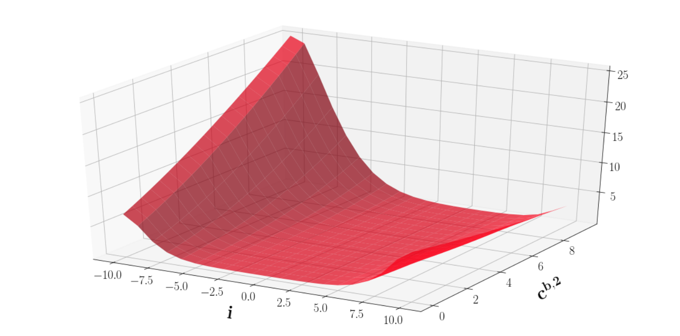
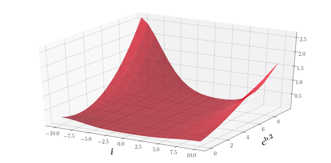
We compare the different value functions associated to each controls in Figures 1, 2 and 3. As expected the control δ2\delta^{2} is optimal and δ0\delta^{0} is sub-optimal compared δ1\delta^{1}. Moreover we observe in Figure 1 that considering an exponential kernel Hawkes model for the order flows leads to a 10%10\% gain compared with a strategy considering that market order flows is a Poisson process. Using two exponentials leads to another 10%10\% gain. This shows the large gain that can arise from taking into account the clustering and long memory properties of market order flows when designing a market making strategy.

Refer to caption
Figure 1: Value functions along the time for controls δ0\delta^{0}, δ1\delta^{1} and δ2\delta^{2} with initial condition ca=(0,10)c^{a}=(0,10), cb=(0,10)c^{b}=(0,10) and i=−10i=-10.
Refer to caption
Figure 2: Difference between the value functions associated to controls δ2\delta^{2} and δ1\delta^{1} for ca=(10,0)c^{a}=(10,0), cb,1=10c^{b,1}=10.
Refer to caption
Figure 3: Difference between the value functions associated to controls δ2\delta^{2} and δ0\delta^{0} for ca=(10,0)c^{a}=(10,0), cb,1=10c^{b,1}=10.

4.2 Numerical illustration of Section 3.4

In this section we use the method presented in Section 3.4 to estimate UKU^{K} at several points when the function KK is the following completely monotone L1L^{1} function:

K⁡(t)=λλ+(t+ε)α​1(t+ε)β​𝟏ℝ+​(t),K(t)=\frac{\lambda}{\lambda+(t+\varepsilon)^{\alpha}}\frac{1}{(t+\varepsilon)^{\beta}}\mathbf{1}_{\mathbb{R}_{+}}(t),

for λ=0.1\lambda=0.1, α=0.7\alpha=0.7, β=0.4\beta=0.4 and ε=0.01\varepsilon=0.01 is a small shift used for numerical purposes.

We explain in Appendix G how to build in this case the sequence (αn,βn)n≥0(\alpha_{n},\beta_{n})_{n\geq 0} given by Lemma 3.1. As in Section 3.4 we note Kn=Kαn,βnK_{n}=K^{\alpha_{n},\beta_{n}}.

For any nn we consider the following elements of ℰKn\mathcal{E}^{K_{n}}

x0n=(0,0,5​Kn,0),x1n=(0,5,5​Kn,0)​ and ​x2n=(0,−5,5​Kn,0)x^{n}_{0}=(0,0,5K^{n},0),~x^{n}_{1}=(0,5,5K^{n},0)\text{ and }x^{n}_{2}=(0,-5,5K^{n},0)

and the following elements of ℰK\mathcal{E}^{K}

x0=(0,0,5​K,0),x1=(0,5,5​K,0)​ and ​x2n=(0,5,5​K,0).x_{0}=(0,0,5K,0),~x_{1}=(0,5,5K,0)\text{ and }x^{n}_{2}=(0,5,5K,0).

According to Proposition 3.1 we have

UKn​(xin)​→n→+∞​UK​(xi)​ for any ​i∈{0,1,2}.U_{K_{n}}(x^{n}_{i})\underset{n\rightarrow+\infty}{\rightarrow}U_{K}(x_{i})\text{ for any }i\in\{0,1,2\}.

This convergence is illustrated in Figure 4. We used the probabilistic representation of [13] to compute the UKn​(xin)U^{K_{n}}(x^{n}_{i}) and UK​(xi)U^{K}(x_{i}), see Appendix H for more details. This proves the tractability of the method presented in Section 3.4.

Refer to caption
Figure 4: Log relative difference between UKn​(xin)U^{K_{n}}(x^{n}_{i}) and UK​(xi)U^{K}(x_{i}) for i∈{0,1,2}i\in\{0,1,2\}. We used T=1T=1 for the computations. In red is the linear regression.

.

Acknowledgments

We thank Thibaut Mastrolia, Mathieu Rosenbaum and Nizar Touzi for many interesting discussions. The author gratefully acknowledges the financial support of the ERC Grant 679836 Staqamof and of the chair Analytics and Models for Regulation.

5 Proofs

In this section we drop the superscript KK for the processes XKX^{K}, θK,a\theta^{K,a} and θK,b\theta^{K,b} to lighten the notations.

5.1 Formal definition of the probability space

In this section we make precise the probability space we are working on. In particular we give a proper definition to 𝔼δ\mathbb{E}^{\delta}. First we define the canonical process and the probability space associated to our stochastic control problem.

  • -

    Consider Ωd\Omega_{d} the set of increasing piecewise constant càdlàg functions from [0,T][0,T] into ℕ\mathbb{N} with jumps equal to 11 and Ωp\Omega_{p} the set of continuous functions from [0,T][0,T] into ℝ\mathbb{R}. We define Ω=Ωp×Ωd2\Omega=\Omega_{p}\times\Omega_{d}^{2}.

  • -

    We let (Wt,Nta,Ntb)t∈[0,T](W_{t},N^{a}_{t},N^{b}_{t})_{t\in[0,T]} be the canonical process on Ω\Omega.

  • -

    The associated filtration is 𝔽=(ℱtp⊗ℱtd⊗ℱtd)t∈[0,T]\mathbb{F}=(\mathcal{F}^{p}_{t}\otimes\mathcal{F}^{d}_{t}\otimes\mathcal{F}^{d}_{t})_{t\in[0,T]} where (ℱtd)t∈[0,T](\mathcal{F}^{d}_{t})_{t\in[0,T]} (resp. (ℱtp)t∈[0,T](\mathcal{F}^{p}_{t})_{t\in[0,T]}) is the right continuous completed filtration associated with NaN^{a} (or NbN^{b}) (resp. WW).

  • -

    We denote by ℙ0\mathbb{P}_{0} the probability measure on (Ω,𝔽)(\Omega,\mathbb{F}) such that (Msa=Nsa−s​λ0,Msb=Nsb−s​λ0)s∈[0,T]\big(M^{a}_{s}=N^{a}_{s}-s\lambda_{0},~M^{b}_{s}=N^{b}_{s}-s\lambda_{0}\big)_{s\in[0,T]}, for λ0>0\lambda_{0}>0, are local martingales and (Ws)s∈[0,T](W_{s})_{s\in[0,T]} is a Brownian motion .

We now introduce some processes we use later in this paper. For a fixed (t,x)∈ℰK(t,x)\in\mathcal{E}^{K} we define Xt,x=(Pt,x,it,x,θt,x;a,θt,x;b)X^{t,x}=(P^{t,x},i^{t,x},\theta^{t,x;a},\theta^{t,x;b}) that is the state of the system after time tt when starting from point (t,x)(t,x). The dynamics of Xt,xX^{t,x} is given on [t,T][t,T] by

d​Pst,x=d⁡(s,Pst,x)​d​s+σ​d​Ws,Ptt,x=p,\displaystyle\mathrm{d}P^{t,x}_{s}=d(s,P_{s}^{t,x})\mathrm{d}s+\sigma\mathrm{d}W_{s},~~P^{t,x}_{t}=p,
d​ist,x=d​Nsa−d​Nsb,itt,x=i,\displaystyle\mathrm{d}i^{t,x}_{s}=\mathrm{d}N^{a}_{s}-\mathrm{d}N^{b}_{s},~~i^{t,x}_{t}=i,
dθst,x;a=K(⋅−s)dNsa,θtt,x;a=θa,\displaystyle\mathrm{d}\theta^{t,x;a}_{s}=K(\cdot-s)\mathrm{d}N^{a}_{s},~~\theta^{t,x;a}_{t}=\theta^{a},
dθst,x;b=K(⋅−s)dNsb,θtt,x;b=θb.\displaystyle\mathrm{d}\theta^{t,x;b}_{s}=K(\cdot-s)\mathrm{d}N^{b}_{s},~~\theta^{t,x;b}_{t}=\theta^{b}.

Using those processes we explicit the change of measure associated to each control process. For this we consider the functions

λa​(t,x,δ)=e−kσ​δa​Φ​(θa​(t))​ and ​λb​(t,x,δ)=e−kσ​δb​Φ​(θb​(t)),\lambda^{a}(t,x,\delta)=e^{-\frac{k}{\sigma}\delta^{a}}\Phi\big(\theta^{a}(t)\big)\text{ and }\lambda^{b}(t,x,\delta)=e^{-\frac{k}{\sigma}\delta^{b}}\Phi\big(\theta^{b}(t)\big),

that represent the ask and bid intensity in the state (t,x)∈ℰK(t,x)\in\mathcal{E}^{K} when the control is δ\delta. For any δ∈𝒜\delta\in\mathcal{A} we define ℙt,x;δ\mathbb{P}^{t,x;\delta} by

d​ℙt,x;δd​ℙ0=LTt,x;δ\frac{\mathrm{d}\mathbb{P}^{t,x;\delta}}{\mathrm{d}\mathbb{P}_{0}}=L_{T}^{t,x;\delta}

where LTt,x;δL_{T}^{t,x;\delta} is the Doléans-Dade exponential of

Zst,x;δ=∫0sλa​(s,Xst,x,δs)−λ0λ0​𝟏s≥t​d​Msa+λb​(s,Xst,x,δs)−λ0λ0​𝟏s≥t​d​Msb.Z^{t,x;\delta}_{s}=\int_{0}^{s}\frac{\lambda^{a}(s,X^{t,x}_{s},\delta_{s})-\lambda_{0}}{\lambda_{0}}\mathbf{1}_{s\geq t}\mathrm{d}M^{a}_{s}+\frac{\lambda^{b}(s,X^{t,x}_{s},\delta_{s})-\lambda_{0}}{\lambda_{0}}\mathbf{1}_{s\geq t}\mathrm{d}M^{b}_{s}.

Since λa​(t,x,δ)≤C⁡(1+‖x‖)\lambda^{a}(t,x,\delta)\leq C(1+\|x\|) and λb​(t,x,δ)≤C⁡(1+‖x‖)\lambda^{b}(t,x,\delta)\leq C(1+\|x\|), by the Corrolary 2.6 in [24], for any (t,x)∈ℰK(t,x)\in\mathcal{E}^{K}, (Lst,x;δ)s∈[t,T](L_{s}^{t,x;\delta})_{s\in[t,T]} is a true ℙ0\mathbb{P}_{0} martingale. Moreover by Theorem III-3.11 in [17] the processes

Mt,x;a,δ=Na−∫t⋅λa​(u,δu,Xut,x)​𝑑u​ and ​Mt,x;b,δ=Nb−∫t⋅λb​(u,δu,Xut,x)​𝑑uM^{t,x;a,\delta}=N^{a}-\int_{t}^{\cdot}\lambda^{a}(u,\delta_{u},X^{t,x}_{u})\mathrm{d}u\text{ and }M^{t,x;b,\delta}=N^{b}-\int_{t}^{\cdot}\lambda^{b}(u,\delta_{u},X^{t,x}_{u})\mathrm{d}u

are ℙt,x;δ\mathbb{P}^{t,x;\delta}-local martingales on [t,T][t,T]. Actually they are true martingales, see Appendix B.1.

For (t,x)∈ℰK(t,x)\in\mathcal{E}^{K} and δ∈𝒜\delta\in\mathcal{A} we note 𝔼t,xδ\mathbb{E}^{\delta}_{t,x} the expectation under the law ℙt,x;δ\mathbb{P}^{t,x;\delta} and note 𝔼δ\mathbb{E}^{\delta} instead of 𝔼0,0δ\mathbb{E}^{\delta}_{0,0}.

Finally, for any FF bounded continuous function, δ∈𝒜\delta\in\mathcal{A} and θ\theta stopping time with values in [t,T][t,T] we have:

𝔼t,xδ​[F⁡(XTt,x)|ℱθ]=𝔼θ,Xθt,xδθ​[F⁡(XTθ,Xθt,x)]\mathbb{E}^{\delta}_{t,x}[F(X^{t,x}_{T})|\mathcal{F}_{\theta}]=\mathbb{E}^{\delta^{\theta}}_{\theta,X^{t,x}_{\theta}}[F(X^{\theta,X^{t,x}_{\theta}}_{T})] (8)

where, δθ\delta^{\theta} is the restriction to [θ,T][\theta,T] of δ\delta. This prove that for any (t,x)∈ℰK(t,x)\in\mathcal{E}^{K} the process (s,Xst,x)s≥t(s,X^{t,x}_{s})_{s\geq t} is Markovian.

5.2 Proof of Theorem 2.1

We proceed in 5 steps.

  1. 1.

    Section 5.2.1: Using a comparison result we show that (𝐇𝐉𝐁)K(\mathbf{HJB})_{K} admits a unique viscosity solution with polynomial growth.

  2. 2.

    Section 5.2.2: For any KK we define UKU^{K} the continuation utility function associated to (3).

  3. 3.

    Section 5.2.3: We prove a dynamic programming principle for UKU^{K}.

  4. 4.

    Section 5.2.4: Using a verification argument we show that UKU^{K} is the unique viscosity solution (with polynomial growth) of (𝐇𝐉𝐁)K(\mathbf{HJB})_{K}.

  5. 5.

    Section 5.2.5: We show that the control given in Equation (5) solves the control problem (3).

5.2.1 Comparison result for (𝐇𝐉𝐁)K(\mathbf{HJB})_{K}

We start by proving a comparison result for bounded solutions, then we extend it to functions with polynomial growth.

Proposition 5.1.

Let U∈U​S​C​(ℰK)U\in USC(\mathcal{E}^{K}) be a bounded from above viscosity sub-solution of (𝐇𝐉𝐁)K(\mathbf{HJB})_{K} and V∈L​S​C​(ℰK)V\in LSC(\mathcal{E}^{K}) be a bounded from below viscosity super-solution of (𝐇𝐉𝐁)K(\mathbf{HJB})_{K} such that U⁡(T,⋅)≤V⁡(T,⋅)U(T,\cdot)\leq V(T,\cdot) then

U≤V​ on ​ℰK.U\leq V\text{ on }\mathcal{E}^{K}.
Proof.

We suppose that there exists some (t0,x0)∈ℰK(t_{0},x_{0})\in\mathcal{E}^{K} such that

U⁡(t0,x0)−V⁡(t0,x0)=δ>0.U(t_{0},x_{0})-V(t_{0},x_{0})=\delta>0.

By hypothesis, necessarily t0∈[0,T)t_{0}\in[0,T). We show that this implies a contradiction. We consider the following quantities

Nε=sup(t,x)∈ℰK​U​(t,x)−V⁡(t,x)−2​ε​‖x‖2N_{\varepsilon}=\underset{(t,x)\in\mathcal{E}^{K}}{\sup}~U(t,x)-V(t,x)-2\varepsilon\|x\|^{2}

and

Nεα=sup(t,x),(t,y)∈ℰK​U​(t,x)−V⁡(t,y)−ε⁡(‖x‖2+‖y‖2)−α​‖x−y‖2.N^{\alpha}_{\varepsilon}=\underset{(t,x),(t,y)\in\mathcal{E}^{K}}{\sup}U(t,x)-V(t,y)-\varepsilon(\|x\|^{2}+\|y\|^{2})-\alpha\|x-y\|^{2}.

The functions UU and −V-V being bounded from above we have

lim‖x‖+‖y‖→+∞​U​(t,x)−V⁡(t,y)−α​‖x−y‖2−ε​‖x‖2−ε​‖y‖2=−∞\underset{\|x\|+\|y\|\rightarrow+\infty}{\lim}~U(t,x)-V(t,y)-\alpha\|x-y\|^{2}-\varepsilon\|x\|^{2}-\varepsilon\|y\|^{2}=-\infty

uniformly in tt. Thus we can restrict the supremums to bounded sets that depends only on ε\varepsilon. More precisely

Nε\displaystyle N_{\varepsilon} =\displaystyle= sup(t,x)∈ℰRK​U​(t,x)−V⁡(t,x)−2​ε​‖x‖2\displaystyle\underset{(t,x)\in\mathcal{E}^{K}_{R}}{\sup}~U(t,x)-V(t,x)-2\varepsilon\|x\|^{2} (9)
Nεα\displaystyle N^{\alpha}_{\varepsilon} =\displaystyle= sup(t,x),(t,y)∈ℰRK​U​(t,x)−V⁡(t,y)−ε⁡(‖x‖2+‖y‖2)−α​‖x−y‖2\displaystyle\underset{(t,x),(t,y)\in\mathcal{E}^{K}_{R}}{\sup}~U(t,x)-V(t,y)-\varepsilon(\|x\|^{2}+\|y\|^{2})-\alpha\|x-y\|^{2} (10)

where RR only depends on ε\varepsilon. Since the set ℰRK\mathcal{E}^{K}_{R} is compact the supremum NεαN_{\varepsilon}^{\alpha} is achieved at some (tεα,xεα,yεα)(t_{\varepsilon}^{\alpha},x_{\varepsilon}^{\alpha},y_{\varepsilon}^{\alpha}). We show at the end of the proof that when α→+∞\alpha\rightarrow+\infty, up to a subsequence, we have

limα→+∞​(tεα,xεα,yεα)=(tε,xε,xε)\underset{\alpha\rightarrow+\infty}{\lim}(t_{\varepsilon}^{\alpha},x_{\varepsilon}^{\alpha},y_{\varepsilon}^{\alpha})=(t_{\varepsilon},x_{\varepsilon},x_{\varepsilon}) (11)

where (tε,xε)(t_{\varepsilon},x_{\varepsilon}) achieves the supremum NεN_{\varepsilon}. We also prove that

limα→+∞​α​‖xεα−yεα‖2=0​, ​limα→0​Nεα=Nε,limε→0​ε​‖xε‖2=0\underset{\alpha\rightarrow+\infty}{\lim}~\alpha\|x_{\varepsilon}^{\alpha}-y_{\varepsilon}^{\alpha}\|^{2}=0\text{, }\underset{\alpha\rightarrow 0}{\lim}~N_{\varepsilon}^{\alpha}=N_{\varepsilon},~\underset{\varepsilon\rightarrow 0}{\lim}~\varepsilon\|x_{\varepsilon}\|^{2}=0 (12)

and that

limε→0​Nε=N=sup(t,x)∈ℰK​U​(t,x)−V⁡(t,x).\underset{\varepsilon\rightarrow 0}{\lim}~N_{\varepsilon}=N=\underset{(t,x)\in\mathcal{E}^{K}}{\sup}~U(t,x)-V(t,x). (13)

A consequence of Equation (13) is that

limα→+∞​(U⁡(tεα,xεα),V⁡(tεα,xεα))=(U⁡(tε,xε),V⁡(tε,xε)).\underset{\alpha\rightarrow+\infty}{\lim}\big(U(t^{\alpha}_{\varepsilon},x^{\alpha}_{\varepsilon}),V(t^{\alpha}_{\varepsilon},x^{\alpha}_{\varepsilon})\big)=\big(U(t_{\varepsilon},x_{\varepsilon}),V(t_{\varepsilon},x_{\varepsilon})\big). (14)

We use the notations xεα=(Pεα,iεα,θεa,α,θεb,α)​ and ​yεα=(Qεα,jεα,βεa,α,βεb,α)x_{\varepsilon}^{\alpha}=(P_{\varepsilon}^{\alpha},i_{\varepsilon}^{\alpha},\theta_{\varepsilon}^{a,\alpha},\theta_{\varepsilon}^{b,\alpha})\text{ and }y_{\varepsilon}^{\alpha}=(Q_{\varepsilon}^{\alpha},j_{\varepsilon}^{\alpha},\beta_{\varepsilon}^{a,\alpha},\beta_{\varepsilon}^{b,\alpha}).

With respect to Lemma D.1, which is an adaptation of the Crandall-Ishi’s lemma to our framework, for any β>0\beta>0 there exists ((λεα,pεα),Aεβ,α,h)∈𝒥¯+​U​(tεα,xεα)\big((\lambda^{\alpha}_{\varepsilon},p^{\alpha}_{\varepsilon}),A^{\beta,\alpha}_{\varepsilon},h)\in\overline{\mathcal{J}}^{+}U(t^{\alpha}_{\varepsilon},x^{\alpha}_{\varepsilon}\big) and ((λ^εα,qεα),Bεβ,α,g)∈𝒥¯−​V​(tεα,yεα)\big((\hat{\lambda}^{\alpha}_{\varepsilon},q^{\alpha}_{\varepsilon}),B^{\beta,\alpha}_{\varepsilon},g)\in\overline{\mathcal{J}}^{-}V(t^{\alpha}_{\varepsilon},y^{\alpha}_{\varepsilon}\big) such that

−(β−1+2​ε+4​α)​I2≤(Aεβ,α00−Bεβ,α)≤(2​ε+β​4​ε2)​I2+(2​α+8​β​(α​ε+α2))​(1−1−11).-(\beta^{-1}+2\varepsilon+4\alpha)I_{2}\leq\begin{pmatrix}A^{\beta,\alpha}_{\varepsilon}&0\\ 0&-B^{\beta,\alpha}_{\varepsilon}\end{pmatrix}\leq(2\varepsilon+\beta 4\varepsilon^{2})I_{2}+\big(2\alpha+8\beta(\alpha\varepsilon+\alpha^{2})\big)\begin{pmatrix}1&-1\\ -1&1\end{pmatrix}.

with

pεα=2​ε​Pεα+2​α​(Pεα−Qεα),qεα=−2​ε​Qεα−2​α​(Qεα−Pεα),λεα=0​ and ​λ^εα=0.p^{\alpha}_{\varepsilon}=2\varepsilon P^{\alpha}_{\varepsilon}+2\alpha(P^{\alpha}_{\varepsilon}-Q^{\alpha}_{\varepsilon}),~q^{\alpha}_{\varepsilon}=-2\varepsilon Q^{\alpha}_{\varepsilon}-2\alpha(Q^{\alpha}_{\varepsilon}-P^{\alpha}_{\varepsilon}),~\lambda^{\alpha}_{\varepsilon}=0\text{ and }\hat{\lambda}^{\alpha}_{\varepsilon}=0.

Remark that for ε\varepsilon small enough

U⁡(tεα,xεα)−V⁡(tεα,yεα)≥δ−ε​‖x0‖2>δ2U(t^{\alpha}_{\varepsilon},x^{\alpha}_{\varepsilon})-V(t^{\alpha}_{\varepsilon},y^{\alpha}_{\varepsilon})\geq\delta-\varepsilon\|x_{0}\|^{2}>\frac{\delta}{2}

We now walk towards a contradiction by showing that

limsupε→0​limsupα→+∞​U​(tεα,xεα)−V⁡(tεα,yεα)≤0.\underset{\varepsilon\rightarrow 0}{\lim\sup}~\underset{\alpha\rightarrow+\infty}{\lim\sup}~U(t^{\alpha}_{\varepsilon},x^{\alpha}_{\varepsilon})-V(t^{\alpha}_{\varepsilon},y^{\alpha}_{\varepsilon})\leq 0.

According to the definition of sub-solution and super-solution we have

F⁡(tεα,xεα,U⁡(tεα,xεα),(λεα,pεα),Aεβ,α,DK​U​(tεα,xεα))≤0F\big(t_{\varepsilon}^{\alpha},x_{\varepsilon}^{\alpha},U(t_{\varepsilon}^{\alpha},x_{\varepsilon}^{\alpha}),(\lambda^{\alpha}_{\varepsilon},p^{\alpha}_{\varepsilon}),A^{\beta,\alpha}_{\varepsilon},D^{K}U(t_{\varepsilon}^{\alpha},x_{\varepsilon}^{\alpha})\big)\leq 0

and

F⁡(tεα,yεα,V⁡(tεα,yεα),(λ^εα,qεα),Bεβ,α,DK​V​(tεα,yεα))≥0.F\big(t_{\varepsilon}^{\alpha},y_{\varepsilon}^{\alpha},V(t_{\varepsilon}^{\alpha},y_{\varepsilon}^{\alpha}),(\hat{\lambda}^{\alpha}_{\varepsilon},q^{\alpha}_{\varepsilon}),B^{\beta,\alpha}_{\varepsilon},D^{K}V(t_{\varepsilon}^{\alpha},y_{\varepsilon}^{\alpha})\big)\geq 0.

By definition of FF:

r⁡(U⁡(tεα,xεα)−V⁡(tεα,yεα))\displaystyle r\big(U(t_{\varepsilon}^{\alpha},x^{\alpha}_{\varepsilon})-V(t_{\varepsilon}^{\alpha},y^{\alpha}_{\varepsilon})\big) ≤F⁡(tεα,xεα,U⁡(tεα,xεα),(λεα,pεα),Aεβ,α,DK​U​(tεα,xεα))\displaystyle\leq F\big(t_{\varepsilon}^{\alpha},x^{\alpha}_{\varepsilon},U(t_{\varepsilon}^{\alpha},x^{\alpha}_{\varepsilon}),(\lambda^{\alpha}_{\varepsilon},p^{\alpha}_{\varepsilon}),A^{\beta,\alpha}_{\varepsilon},D^{K}U(t_{\varepsilon}^{\alpha},x^{\alpha}_{\varepsilon})\big)
−F⁡(tεα,xεα,V⁡(tεα,yεα),(λεα,pεα),Aεβ,α,DK​U​(tεα,xεα)),\displaystyle~~~~~~-F\big(t_{\varepsilon}^{\alpha},x^{\alpha}_{\varepsilon},V(t_{\varepsilon}^{\alpha},y^{\alpha}_{\varepsilon}),(\lambda^{\alpha}_{\varepsilon},p^{\alpha}_{\varepsilon}),A^{\beta,\alpha}_{\varepsilon},D^{K}U(t_{\varepsilon}^{\alpha},x^{\alpha}_{\varepsilon})\big),

thus

r⁡(U⁡(tεα,xεα)−V⁡(tεα,yεα))\displaystyle r\big(U(t_{\varepsilon}^{\alpha},x^{\alpha}_{\varepsilon})-V(t_{\varepsilon}^{\alpha},y^{\alpha}_{\varepsilon})\big) ≤F⁡(tεα,yεα,V⁡(tεα,yεα),λ^εα,qεα,Bεβ,α,DK​V​(tεα,yεα))\displaystyle\leq F(t_{\varepsilon}^{\alpha},y^{\alpha}_{\varepsilon},V(t_{\varepsilon}^{\alpha},y^{\alpha}_{\varepsilon}),\hat{\lambda}^{\alpha}_{\varepsilon},q^{\alpha}_{\varepsilon},B^{\beta,\alpha}_{\varepsilon},D^{K}V(t_{\varepsilon}^{\alpha},y^{\alpha}_{\varepsilon}))
−F⁡(tεα,xεα,V⁡(tεα,yεα),λεα,pεα,Aεβ,α,DK​U​(tεα,xεα))\displaystyle~~~~~~-F(t_{\varepsilon}^{\alpha},x^{\alpha}_{\varepsilon},V(t_{\varepsilon}^{\alpha},y^{\alpha}_{\varepsilon}),\lambda^{\alpha}_{\varepsilon},p^{\alpha}_{\varepsilon},A^{\beta,\alpha}_{\varepsilon},D^{K}U(t_{\varepsilon}^{\alpha},x^{\alpha}_{\varepsilon}))
≤d⁡(tεα,Pεα)​pεα−d⁡(tεα,Qεα)​qεα+12​σ2​Aεα−12​σ2​Bεα\displaystyle\leq d(t_{\varepsilon}^{\alpha},P^{\alpha}_{\varepsilon})p^{\alpha}_{\varepsilon}-d(t_{\varepsilon}^{\alpha},Q^{\alpha}_{\varepsilon})q^{\alpha}_{\varepsilon}+\frac{1}{2}\sigma^{2}A^{\alpha}_{\varepsilon}-\frac{1}{2}\sigma^{2}B^{\alpha}_{\varepsilon}
+H⁡(tεα,yεα,DK​V​(tεα,yεα))−H⁡(tεα,xεα,DK​U​(tεα,xεα))\displaystyle~~~~~~+H(t^{\alpha}_{\varepsilon},y^{\alpha}_{\varepsilon},D^{K}V(t^{\alpha}_{\varepsilon},y^{\alpha}_{\varepsilon}))-H(t^{\alpha}_{\varepsilon},x^{\alpha}_{\varepsilon},D^{K}U(t^{\alpha}_{\varepsilon},x^{\alpha}_{\varepsilon}))

where

H⁡(t,x,I)=−supδ∈ℝ+​Φ​(θa​(t))​e−σk​δ​(δ+I1)−supδ∈ℝ+​Φ​(θb​(t))​e−σk​δ​(δ+I2)+g⁡(i,p).H(t,x,I)=-\underset{\delta\in\mathbb{R}_{+}}{\sup}\Phi\big(\theta^{a}(t)\big)e^{-\frac{\sigma}{k}\delta}(\delta+I_{1})-\underset{\delta\in\mathbb{R}_{+}}{\sup}\Phi\big(\theta^{b}(t)\big)e^{-\frac{\sigma}{k}\delta}(\delta+I_{2})+g(i,p).

Note that the function HH is Lipschitz continuous. Taking β=α−1\beta=\alpha^{-1} we get

σ2​Aεβ,α−σ2​Bεβ,α≤2​(2​ε+α−1​4​ε2)​σ2.\sigma^{2}A^{\beta,\alpha}_{\varepsilon}-\sigma^{2}B^{\beta,\alpha}_{\varepsilon}\leq 2(2\varepsilon+\alpha^{-1}4\varepsilon^{2})\sigma^{2}.

The RHS can be taken arbitrarly small when α→+∞\alpha\rightarrow+\infty and ε→0\varepsilon\rightarrow 0 by Equation (12). Using the Lipschitz property of dd we have

d⁡(tεα,Pεα)​pεα−d⁡(tεα,Qεα)​qεα\displaystyle d(t_{\varepsilon}^{\alpha},P^{\alpha}_{\varepsilon})p^{\alpha}_{\varepsilon}-d(t_{\varepsilon}^{\alpha},Q^{\alpha}_{\varepsilon})q^{\alpha}_{\varepsilon} =2​ε​(d⁡(tεα,Pεα)​Pεα+d⁡(tεα,Qεα)​Qεα)+2​α​(Pεα−Qεα)​(d⁡(tεα,Pεα)−d⁡(tεα,qεα))\displaystyle=2\varepsilon\big(d(t_{\varepsilon}^{\alpha},P^{\alpha}_{\varepsilon})P^{\alpha}_{\varepsilon}+d(t_{\varepsilon}^{\alpha},Q^{\alpha}_{\varepsilon})Q^{\alpha}_{\varepsilon}\big)+2\alpha(P^{\alpha}_{\varepsilon}-Q^{\alpha}_{\varepsilon})\big(d(t_{\varepsilon}^{\alpha},P^{\alpha}_{\varepsilon})-d(t_{\varepsilon}^{\alpha},q^{\alpha}_{\varepsilon})\big)
≤2​ε​C​(1+‖yεα‖2+‖xεα‖2)+C​α​‖xεα−yεα‖2.\displaystyle\leq 2\varepsilon C(1+\|y^{\alpha}_{\varepsilon}\|^{2}+\|x^{\alpha}_{\varepsilon}\|^{2})+C\alpha\|x^{\alpha}_{\varepsilon}-y^{\alpha}_{\varepsilon}\|^{2}.

Here the RHS goes to zero when α→+∞\alpha\rightarrow+\infty and ε→0\varepsilon\rightarrow 0 due to Equation (12). Finally, by Equation (14) and since UU (resp. VV) is a USC (resp. LSC) function and HH is continuous and decreasing with respect to its last variable we have

limsupα→+∞​H​(tεα,yεα,DK​V​(tεα,yεα))−H⁡(tεα,xεα,DK​U​(tεα,xεα))≤H⁡(tε,xε,DK​V​(tε,xε))−H⁡(tε,xε,DK​U​(tε,xε)).\underset{\alpha\rightarrow+\infty}{\lim\sup}~H(t_{\varepsilon}^{\alpha},y_{\varepsilon}^{\alpha},D^{K}V(t_{\varepsilon}^{\alpha},y_{\varepsilon}^{\alpha}))-H(t_{\varepsilon}^{\alpha},x_{\varepsilon}^{\alpha},D^{K}U(t_{\varepsilon}^{\alpha},x_{\varepsilon}^{\alpha}))\leq H\big(t_{\varepsilon},x_{\varepsilon},D^{K}V(t_{\varepsilon},x_{\varepsilon})\big)-H\big(t_{\varepsilon},x_{\varepsilon},D^{K}U(t_{\varepsilon},x_{\varepsilon})\big).

Remark that for any zz such that (tε,xε+z)∈ℰK(t_{\varepsilon},x_{\varepsilon}+z)\in\mathcal{E}^{K} we have by definition of (tε,xε)(t_{\varepsilon},x_{\varepsilon})

U⁡(tε,xε)−V⁡(tε,xε)−2​ε​‖xε‖2≥U⁡(tε,xε+z)−V⁡(tε,xε+z)−2​ε​‖xε+z‖2.U(t_{\varepsilon},x_{\varepsilon})-V(t_{\varepsilon},x_{\varepsilon})-2\varepsilon\|x_{\varepsilon}\|^{2}\geq U(t_{\varepsilon},x_{\varepsilon}+z)-V(t_{\varepsilon},x_{\varepsilon}+z)-2\varepsilon\|x_{\varepsilon}+z\|^{2}.

Consequently we have

V⁡(tε,xε+z)−V⁡(tε,xε)≥U⁡(tε,xε+z)−U⁡(tε,xε)−2​ε​(‖xε+z‖2−‖xε‖2)V(t_{\varepsilon},x_{\varepsilon}+z)-V(t_{\varepsilon},x_{\varepsilon})\geq U(t_{\varepsilon},x_{\varepsilon}+z)-U(t_{\varepsilon},x_{\varepsilon})-2\varepsilon\big(\|x_{\varepsilon}+z\|^{2}-\|x_{\varepsilon}\|^{2}\big)

and so

DKV(tε,xε)≤DK(U−2ε∥⋅∥)(tε,xε).D^{K}V(t_{\varepsilon},x_{\varepsilon})\leq D^{K}(U-2\varepsilon\|\cdot\|)(t_{\varepsilon},x_{\varepsilon}).

The monotony and Lipschitz regularity of HH implies

limsupα→+∞\displaystyle\underset{\alpha\rightarrow+\infty}{\lim\sup}~ H⁡(tεα,yεα,DK​V​(tεα,yεα))−H⁡(tεα,xεα,DK​U​(tεα,xεα))\displaystyle H(t_{\varepsilon}^{\alpha},y_{\varepsilon}^{\alpha},D^{K}V(t_{\varepsilon}^{\alpha},y_{\varepsilon}^{\alpha}))-H(t_{\varepsilon}^{\alpha},x_{\varepsilon}^{\alpha},D^{K}U(t_{\varepsilon}^{\alpha},x_{\varepsilon}^{\alpha}))
≤H(xε,DK(U−2ε∥⋅∥)(tε,xε))−H(xε,DKU(tε,xε))\displaystyle~~~\leq H\big(x_{\varepsilon},D^{K}(U-2\varepsilon\|\cdot\|)(t_{\varepsilon},x_{\varepsilon})\big)-H\big(x_{\varepsilon},D^{K}U(t_{\varepsilon},x_{\varepsilon})\big)
≤Cε∥xε∥∥DK∥⋅∥2(tε,xε)∥.\displaystyle~~~\leq C\varepsilon\|x_{\varepsilon}\|\Big\|D^{K}\|\cdot\|^{2}(t_{\varepsilon},x_{\varepsilon})\Big\|.

Notice that for any x∈ℰKx\in\mathcal{E}^{K}

DK∥⋅∥2(x)=(∥θa+K(⋅−t)∥21−∥θa∥21+|i+1|2−|i|2∥θb+K(⋅−t)∥21−∥θb∥21+|i−1|2−|i|2)=(∥K(⋅−t)∥21+2∥K(⋅−t)∥1∥θa∥1+1+2i∥K(⋅−t)∥21+2∥K(⋅−t)∥1∥θb∥1+1−2i),\begin{array}[]{ll}D^{K}\|\cdot\|^{2}(x)&=\begin{pmatrix}\|\theta^{a}+K(\cdot-t)\|^{2}_{1}-\|\theta^{a}\|^{2}_{1}+|i+1|^{2}-|i|^{2}\\ \|\theta^{b}+K(\cdot-t)\|^{2}_{1}-\|\theta^{b}\|^{2}_{1}+|i-1|^{2}-|i|^{2}\end{pmatrix}\\ &=\begin{pmatrix}\|K(\cdot-t)\|^{2}_{1}+2\|K(\cdot-t)\|_{1}\|\theta^{a}\|_{1}+1+2i\\ \|K(\cdot-t)\|^{2}_{1}+2\|K(\cdot-t)\|_{1}\|\theta^{b}\|_{1}+1-2i\end{pmatrix},\end{array}

thus there exists C>0C>0 such that ∥DK∥⋅∥2(t,x)∥≤C(1+∥x∥)\big\|D^{K}\|\cdot\|^{2}(t,x)\big\|\leq C(1+\|x\|). Consequently we get

limsupα→+∞​H​(tεα,yεα,DK​V​(tεα,yεα))−H⁡(tεα,xεα,DK​U​(tεα,xεα))≤C​ε​(1+‖xε‖2)\displaystyle\underset{\alpha\rightarrow+\infty}{\lim\sup}~H(t_{\varepsilon}^{\alpha},y_{\varepsilon}^{\alpha},D^{K}V(t_{\varepsilon}^{\alpha},y_{\varepsilon}^{\alpha}))-H(t_{\varepsilon}^{\alpha},x_{\varepsilon}^{\alpha},D^{K}U(t_{\varepsilon}^{\alpha},x_{\varepsilon}^{\alpha}))\leq C\varepsilon(1+\|x_{\varepsilon}\|^{2})

that goes to zero when taking the limit ε→0\varepsilon\rightarrow 0. Finally we have shown that

limsupε→0​limsupα→+∞​U​(tεα,xεα)−V⁡(tεα,yεα)≤0,\underset{\varepsilon\rightarrow 0}{\lim\sup}~\underset{\alpha\rightarrow+\infty}{\lim\sup}~U(t^{\alpha}_{\varepsilon},x^{\alpha}_{\varepsilon})-V(t^{\alpha}_{\varepsilon},y^{\alpha}_{\varepsilon})\leq 0,

which is a contradiction.

We finally prove the statements (11), (12) and (13). We consider (tε,xε,yε)∈(tεα,xεα,yεα)α≥0¯(t_{\varepsilon},x_{\varepsilon},y_{\varepsilon})\in\overline{(t^{\alpha}_{\varepsilon},x^{\alpha}_{\varepsilon},y^{\alpha}_{\varepsilon})_{\alpha\geq 0}} that exists since ℰK\mathcal{E}^{K} is compact. Since Nεα≥NεN^{\alpha}_{\varepsilon}\geq N_{\varepsilon} then necessarily xε=yεx_{\varepsilon}=y_{\varepsilon}. We now prove the first limit of (12) and that (tε,xε)(t_{\varepsilon},x_{\varepsilon}) corresponds to a point where the supremum NεN_{\varepsilon} is achieved. Passing to the lower limit we get

U⁡(tε,xε)−V⁡(tε,xε)−2​ε​‖xε‖2−limsupα→+∞​α​‖xεα−yεα‖2≥Nε.U(t_{\varepsilon},x_{\varepsilon})-V(t_{\varepsilon},x_{\varepsilon})-2\varepsilon\|x_{\varepsilon}\|^{2}-\underset{\alpha\rightarrow+\infty}{\lim\sup}~\alpha\|x^{\alpha}_{\varepsilon}-y^{\alpha}_{\varepsilon}\|^{2}\geq N_{\varepsilon}.

Hence by definition of NεN_{\varepsilon} we necessarily have that limα→+∞​α​‖xεα−yεα‖2=0\underset{\alpha\rightarrow+\infty}{\lim}~\alpha\|x^{\alpha}_{\varepsilon}-y^{\alpha}_{\varepsilon}\|^{2}=0 and that

Nε=U⁡(tε,xε)−V⁡(tε,xε)−2​ε​‖xε‖2.N_{\varepsilon}=U(t_{\varepsilon},x_{\varepsilon})-V(t_{\varepsilon},x_{\varepsilon})-2\varepsilon\|x_{\varepsilon}\|^{2}.

To conclude we show that Nε→NN_{\varepsilon}\rightarrow N and that ε​‖xε‖2→0\varepsilon\|x_{\varepsilon}\|^{2}\rightarrow 0. For ξ>0\xi>0 consider (t,x)(t,x) that is ξ\xi-optimal in the definition of NN:

U⁡(t,x)−V⁡(t,x)≥N−ξ.U(t,x)-V(t,x)\geq N-\xi.

For ε\varepsilon small enough 2​ε​‖x‖22\varepsilon\|x\|^{2} is lower than ξ\xi, and we get

N≥Nε≥U⁡(t,x)−V⁡(t,x)−2​ε​‖x‖2≥N−2​ξ.N\geq N_{\varepsilon}\geq U(t,x)-V(t,x)-2\varepsilon\|x\|^{2}\geq N-2\xi.

Therefore we get convergence of NεN_{\varepsilon} towards NN and as consequence

U⁡(tε,xε)−V⁡(tε,xε)−2​ε​‖xε‖2→N.U(t_{\varepsilon},x_{\varepsilon})-V(t_{\varepsilon},x_{\varepsilon})-2\varepsilon\|x_{\varepsilon}\|^{2}\rightarrow N.

Since for any ε\varepsilon we have

N≥U⁡(tε,xε)−V⁡(tε,xε)≥U⁡(tε,xε)−V⁡(tε,xε)−2​ε​‖xε‖2=Nε,N\geq U(t_{\varepsilon},x_{\varepsilon})-V(t_{\varepsilon},x_{\varepsilon})\geq U(t_{\varepsilon},x_{\varepsilon})-V(t_{\varepsilon},x_{\varepsilon})-2\varepsilon\|x_{\varepsilon}\|^{2}=N_{\varepsilon},

we get that ε​‖xε‖2→0\varepsilon\|x_{\varepsilon}\|^{2}\rightarrow 0. This concludes the proof.

∎

We now extend Proposition 5.1 to the case of functions with polynomial growth.

Proposition 5.2.

Let U∈U​S​C​(ℰK)U\in USC(\mathcal{E}^{K}) with polynomial growth be a viscosity sub-solution of Equation (𝐇𝐉𝐁)K(\mathbf{HJB})_{K} and V∈L​S​C​(ℰK)V\in LSC(\mathcal{E}^{K}) with polynomial growth be a viscosity super-solution of Equation (H​J​B)K(HJB)_{K} such that U⁡(T,⋅)≤V⁡(T,⋅)U(T,\cdot)\leq V(T,\cdot). Then

U≤V​ on ​ℰK.U\leq V\text{ on }\mathcal{E}^{K}.
Proof.

There exists k>0k>0 such that

lim‖x‖→+∞​|U⁡(t,x)|+|V⁡(t,x)|1+‖x‖k=0.\underset{\|x\|\rightarrow+\infty}{\lim}~\frac{|U(t,x)|+|V(t,x)|}{1+\|x\|^{k}}=0.

We introduce the following function

w⁡(t,x)=eM⁡(T−t)​(1+‖x‖2​k),w(t,x)=e^{M(T-t)}(1+\|x\|^{2k}),

where MM is a positive constant. We have

DK​w​(t,x)=eM⁡(T−t)​(P2​k−111​(‖θa‖1)P2​k−112​(i)P2​k−121​(‖θb‖1)P2​k−122​(i))D^{K}w(t,x)=e^{M(T-t)}\begin{pmatrix}P^{11}_{2k-1}(\|\theta^{a}\|_{1})&P^{12}_{2k-1}(i)\\ P^{21}_{2k-1}(\|\theta^{b}\|_{1})&P^{22}_{2k-1}(i)\end{pmatrix}

with (P2​k−1i​j)i,j∈{1,2}(P^{ij}_{2k-1})_{i,j\in\{1,2\}} polynomials with degree 2​k−12k-1. Consequently for some C>0C>0

‖x‖​‖DK​w​(t,x)‖≤C​w​(t,x).\|x\|\|D^{K}w(t,x)\|\leq Cw(t,x).

We have

σ2​∂P2w⁡(t,x)≤C⁡(1+‖x‖2)​eM⁡(T−t)​Q2​k−2​(‖x‖)≤C​w​(t,x)\sigma^{2}\partial^{2}_{P}w(t,x)\leq C(1+\|x\|^{2})e^{M(T-t)}Q_{2k-2}(\|x\|)\leq Cw(t,x)

and

d⁡(t,x)​∂Pw⁡(t,x)≤eM⁡(T−t)​C​(1+‖x‖)​Q2​k−1​(‖x‖)≤C​w​(t,x)d(t,x)\partial_{P}w(t,x)\leq e^{M(T-t)}C(1+\|x\|)Q_{2k-1}(\|x\|)\leq Cw(t,x)

where Q2​k−2Q_{2k-2} and Q2​k−1Q_{2k-1} are two polynomials with respective degree 2​k−22k-2 and 2​k−12k-1. Consequently for any constant BB

−∂tw(t,x)−d(t,x)∂Pw(t,x)−12σ2∂P2w(t,x)−B∥x∥∥DKw(t,x)∥≥w(t,x)(M−C)-\partial_{t}w(t,x)-d(t,x)\partial_{P}w(t,x)-\frac{1}{2}\sigma^{2}\partial^{2}_{P}w(t,x)-B\|x\|\|D^{K}w(t,x)\|\geq w(t,x)(M-C)

which is positive for MM large enough. Hence for any ε>0\varepsilon>0 the function U−ε​wU-\varepsilon w is a bounded from above viscosity sub-solution of Equation (𝐇𝐉𝐁)K(\mathbf{HJB})_{K}. Indeed if U−ε​w<ϕU-\varepsilon w<\phi then U<ϕ+ε​wU<\phi+\varepsilon w consequently

F⁡(t,x,U⁡(t,x),∇(ϕ+ε​w)​(t,x),∂p​p2(ϕ+ε​w)​(t,x),DK​U​(t,x))≤0.F\big(t,x,U(t,x),\nabla(\phi+\varepsilon w)(t,x),\partial^{2}_{pp}(\phi+\varepsilon w)(t,x),D^{K}U(t,x)\big)\leq 0.

We have for MM large enough

F⁡(CLOSE\displaystyle F\big( OPENt,x,U⁡(t,x)−ε​w​(t,x),∇ϕ​(t,x),∂p​p2ϕ⁡(t,x),DK​(U−ε​w)​(t,x))\displaystyle t,x,U(t,x)-\varepsilon w(t,x),\nabla\phi(t,x),\partial_{pp}^{2}\phi(t,x),D^{K}(U-\varepsilon w)(t,x)\big)
−\displaystyle- F⁡(t,x,U⁡(t,x),(∇(ϕ+ε​w)​(t,x),∂p​p2(ϕ+ε​w)​(t,x),DK​U​(t,x))CLOSE\displaystyle F\big(t,x,U(t,x),(\nabla(\phi+\varepsilon w)(t,x),\partial^{2}_{pp}(\phi+\varepsilon w)(t,x),D^{K}U(t,x)\big)
≤ε(−rw(t,x)+(∂t+d∂P+12σ2∂p​p2)w(t,x)+C∥x∥∥DKw(t,x)∥)\displaystyle\leq\varepsilon\big(-rw(t,x)+(\partial_{t}+d\partial_{P}+\frac{1}{2}\sigma^{2}\partial_{pp}^{2})w(t,x)+C\|x\|\|D^{K}w(t,x)\|\big)
<0.\displaystyle<0.

It implies that

F⁡(t,x,U⁡(t,x)−ε​w​(t,x),(∂tϕ⁡(t,x),∂pϕ⁡(t,x)),∂p​p2ϕ⁡(t,x),DK​(U−ε​w)​(t,x))≤0.F\big(t,x,U(t,x)-\varepsilon w(t,x),(\partial_{t}\phi(t,x),\partial_{p}\phi(t,x)),\partial_{pp}^{2}\phi(t,x),D^{K}(U-\varepsilon w)(t,x)\big)\leq 0.

We show in the same way that V+ε​wV+\varepsilon w is a bounded from below viscosity super-solution. Then from Proposition 5.1 we have

U−ε​w≤V+ε​wU-\varepsilon w\leq V+\varepsilon w

and taking ε\varepsilon to 00 we get the stated result. ∎

An immediate consequence from Proposition 5.2 is that there exists a unique viscosity solution with polynomial growth to (𝐇𝐉𝐁)K(\mathbf{HJB})_{K}. We now prove the existence of such solution using a verification argument.

5.2.2 Definition of the continuation utility function

For (t,x)∈ℰK(t,x)\in\mathcal{E}^{K} and δ∈𝒜\delta\in\mathcal{A} we define

JK​(t,x,δ)=𝔼t,xδ​[G⁡(iTt,x,PTt,x)​e−r⁡(T−t)+∫tTe−r⁡(s−t)​g~​(s,Xst,x,δs)​𝑑s]J^{K}(t,x;\delta)=\mathbb{E}_{t,x}^{\delta}[G(i^{t,x}_{T},P^{t,x}_{T})e^{-r(T-t)}+\int_{t}^{T}e^{-r(s-t)}\tilde{g}(s,X^{t,x}_{s},\delta_{s})\mathrm{d}s]

where

g~​(s,x,δ)=g⁡(i,P)+δa​λa​(s,x,δ)+δb​λb​(s,x,δ).\tilde{g}(s,x,\delta)=g(i,P)+\delta^{a}\lambda^{a}(s,x,\delta)+\delta^{b}\lambda^{b}(s,x,\delta).

We also define

UK​(t,x)=supδ∈𝒜​JK​(t,x,δ)U^{K}(t,x)=\underset{\delta\in\mathcal{A}}{\sup}~J^{K}(t,x;\delta) (15)

that is the maximal utility than can expect a market maker starting its trading from time tt with initial market condition given by xx. By Lemma B.1 we get that UKU^{K} has polynomial growth. More precisely there exists a positive constant κ\kappa such that

UK​(t,x)≤κ⁡(1+‖x‖2).U^{K}(t,x)\leq\kappa(1+\|x\|^{2}).

We also define

𝒜t={δ∈𝒜 s.t. δ is independent of ℱt},\mathcal{A}_{t}=\{\delta\in\mathcal{A}\text{ s.t. }\delta\text{ is independent of }\mathcal{F}_{t}\},

the set of controls starting from tt and independent from the past. Since under ℙ0\mathbb{P}_{0} the processes NaN^{a} and NbN^{b} have independent increments, using the same arguments than in Remark 2.2-(i​v)(iv) in [25] we get

UK​(t,x)=supδ∈𝒜t​JK​(t,x,δ).U^{K}(t,x)=\underset{\delta\in\mathcal{A}_{t}}{\sup}J^{K}(t,x;\delta).

In the next sections we show that the function UKU^{K} is the unique viscosity solution with polynomial growth to (𝐇𝐉𝐁)K(\mathbf{HJB})_{K} . For this we prove a dynamic programming principle for UKU^{K} and then conclude using a verification argument.

5.2.3 Dynamic programming principle

Consider the lower and upper semi-continuous version of UKU^{K}:

U∗K(x)=liminfy→xUK(y) and UK∗(x)=limsupy→xUK(y).U_{*}^{K}(x)=\underset{y\rightarrow x}{\lim\inf}~U^{K}(y)\text{ and }U^{K*}(x)=\underset{y\rightarrow x}{\lim\sup}~U^{K}(y).

Inspired by [25] we prove the following dynamic programming principle.

Theorem 5.1.

Let (t,x)∈ℰK(t,x)\in\mathcal{E}^{K} be fixed and {θδ,δ∈𝒜t}\{\theta^{\delta},~\delta\in\mathcal{A}_{t}\} be a family of finite stopping times with values in [t,T][t,T]. Assume that for any δ\delta, (Xst,x​𝟏s∈[t,θδ])s∈[0,T](X^{t,x}_{s}\mathbf{1}_{s\in[t,\theta^{\delta}]})_{s\in[0,T]} is L∞L^{\infty}-bounded. Then we have

UK​(t,x)≥supδ∈𝒜t​𝔼δ​[e−r⁡(θδ−t)​U∗K​(θδ,Xθδt,x)+∫tθδe−r⁡(s−t)​g~​(s,Xst,x,δs)​𝑑s]U^{K}(t,x)\geq\underset{\delta\in\mathcal{A}_{t}}{\sup}~\mathbb{E}^{\delta}[e^{-r(\theta^{\delta}-t)}U^{K}_{*}(\theta^{\delta},X^{t,x}_{\theta^{\delta}})+\int_{t}^{\theta^{\delta}}e^{-r(s-t)}\tilde{g}(s,X^{t,x}_{s},\delta_{s})\mathrm{d}s]

and

UK(t,x)≤supδ∈𝒜t𝔼δ[e−r⁡(θδ−t)UK∗(θδ,Xθδt,x)+∫tθδe−r⁡(s−t)g~(s,Xst,x,δs)ds].U^{K}(t,x)\leq\underset{\delta\in\mathcal{A}_{t}}{\sup}~\mathbb{E}^{\delta}[e^{-r(\theta^{\delta}-t)}U^{K*}(\theta^{\delta},X^{t,x}_{\theta^{\delta}})+\int_{t}^{\theta^{\delta}}e^{-r(s-t)}\tilde{g}(s,X^{t,x}_{s},\delta_{s})\mathrm{d}s].

The proof of Theorem 5.1 is the same as the one of Theorem 2.3 in [25]. However since we are working on non-standard domains we write the proof for the sake of completeness.

Proof.

We first show the first inequality. We consider a continuous function ψ\psi such that UK≥ψU^{K}\geq\psi. By definition of UKU^{K} for any (t,x)∈ℰK(t,x)\in\mathcal{E}^{K} there is an admissible control δt,x,ε∈𝒜t\delta^{t,x,\varepsilon}\in\mathcal{A}_{t} that is ε\varepsilon optimal:

JK​(t,x,δt,x,ε)≥UK​(t,x)−ε.J^{K}(t,x;\delta^{t,x,\varepsilon})\geq U^{K}(t,x)-\varepsilon.

Using Fatou’s lemma and the fact that GG and g~\tilde{g} are lower semi-continuous we get that JK​(⋅,δt,x,ε)J^{K}(\cdot;\delta^{t,x,\varepsilon}) is a lower semi-continuous function. Then ψ\psi being upper semi continuous we can find a family of positive real (rt,x)t,x∈ℰK\big(r_{t,x}\big)_{t,x\in\mathcal{E}^{K}} such that for any (t,x)∈ℰK(t,x)\in\mathcal{E}^{K} we have

ψ⁡(t,x)−ψ⁡(s,y)≥−ε​ and ​JK​(t,x,δt,x,ε)−JK​(s,y,δt,x,ε)≤ε, for ​(s,y)∈B⁡(t,x,rt,x)\psi(t,x)-\psi(s,y)\geq-\varepsilon\text{ and }J^{K}(t,x;\delta^{t,x,\varepsilon})-J^{K}(s,y;\delta^{t,x,\varepsilon})\leq\varepsilon,\text{ for }(s,y)\in B(t,x;r_{t,x})

where

B(t,x;r)={(s,y)∈ℰK s.t. s∈(t−r,t),∥x−y∥<r}.B(t,x;r)=\{(s,y)\in\mathcal{E}^{K}\text{ s.t. }s\in(t-r,t),~\|x-y\|<r\}.

The system (B⁡(t,x,rt,x))t,x∈ℰ(B(t,x;r_{t,x}))_{t,x\in\mathcal{E}} forms an open covering of ℰK\mathcal{E}^{K}. With the topology it is endowed ℰK\mathcal{E}^{K} is second countable since [0,T]×ℝ×ℤ×𝕃1×𝕃1[0,T]\times\mathbb{R}\times\mathbb{Z}\times\mathbb{L}_{1}\times\mathbb{L}_{1} is second countable. Hence by the Lindelöf covering Theorem we can extract from (B⁡(t,x,r⁡(t,x)))(t,x)∈ℰK\big(B(t,x;r(t,x))\big)_{(t,x)\in\mathcal{E}^{K}} a countable subfamily that covers ℰK\mathcal{E}^{K}. Thus we have (ti,xi,ri)i∈ℕ(t_{i},x_{i},r_{i})_{i\in\mathbb{N}} such that

ℰK⊂⋃i∈ℕB⁡(ti,xi,ri).\mathcal{E}^{K}\subset\bigcup_{i\in\mathbb{N}}B(t_{i},x_{i};r_{i}).

Set An=⋃0≤i≤nAiA^{n}=\bigcup_{0\leq i\leq n}A_{i}. Consider A0={T}×𝒳TK,C−1=∅A_{0}=\{T\}\times\mathcal{X}^{K}_{T},~C_{-1}=\emptyset and define the sequence

Ai+1=B⁡(ti+1,xi+1,ri+1)\Ci, where ​Ci=Ci−1∪Ai,i≥0.A_{i+1}=B(t_{i+1},x_{i+1};r_{i+1})\backslash C_{i},\text{ where }C_{i}=C_{i-1}\cup A_{i},~i\geq 0.

Now fix δ∈𝒜t\delta\in\mathcal{A}_{t}. With the above construction, we have (θδ,Xθδt,x)∈∪i≥0Ai(\theta^{\delta},X^{t,x}_{\theta^{\delta}})\in\cup_{i\geq 0}A_{i} and for i≥1i\geq 1, we have

JK​(⋅,δti,xi,ε)≥ψ−3​ε​ on ​Ai.J^{K}(\cdot;\delta^{t_{i},x_{i},\varepsilon})\geq\psi-3\varepsilon\text{ on }A_{i}.

We define the control process δε,n\delta^{\varepsilon,n} by

δsε,n=𝟏[t,θδ]​(s)​δs+𝟏(θδ,T]​(s)​(𝟏Anc​(θδ,Xθδt,x)​δs+∑i=1n𝟏Ai​(θδ,Xθδt,x)​δsti,xi,ε).\delta^{\varepsilon,n}_{s}=\mathbf{1}_{[t,\theta^{\delta}]}(s)\delta_{s}+\mathbf{1}_{(\theta^{\delta},T]}(s)\big(\mathbf{1}_{{A^{n}}^{c}}(\theta^{\delta},X^{t,x}_{\theta^{\delta}})\delta_{s}+\sum_{i=1}^{n}\mathbf{1}_{A_{i}}(\theta^{\delta},X^{t,x}_{\theta^{\delta}})\delta^{t_{i},x_{i},\varepsilon}_{s}\big).

The control δε,n\delta^{\varepsilon,n} is in 𝒜t\mathcal{A}_{t}. By Equation (8) we have

𝔼t,xδε,n[G(iTt,x,PTt,x)e−r⁡(T−t)\displaystyle\mathbb{E}_{t,x}^{\delta^{\varepsilon,n}}[G(i_{T}^{t,x},P^{t,x}_{T})e^{-r(T-t)} +∫tTe−r⁡(s−t)g~(s,Xst,x,δs)ds|ℱθδ]𝟏An(θ,Xθδt,x)\displaystyle+\int_{t}^{T}e^{-r(s-t)}\tilde{g}(s,X^{t,x}_{s},\delta_{s})\mathrm{d}s|\mathcal{F}_{\theta^{\delta}}]\mathbf{1}_{A^{n}}(\theta,X^{t,x}_{\theta^{\delta}})
=\displaystyle= (UK​(T,XTt,x)​e−r⁡(T−t)+∫tTe−r⁡(s−t)​g~​(s,Xst,x,δs)​𝑑s)​𝟏A0​(θδ,Xθδt,x)\displaystyle\big(U^{K}(T,X_{T}^{t,x})e^{-r(T-t)}+\int_{t}^{T}e^{-r(s-t)}\tilde{g}(s,X^{t,x}_{s},\delta_{s})\mathrm{d}s\big)\mathbf{1}_{A_{0}}(\theta^{\delta},X^{t,x}_{\theta^{\delta}})
+∑i=1n(e−r⁡(θδ−t)JK(θδ,Xθδt,x;δti,xi,ε)+∫tθδe−r⁡(s−t)g~(s,Xst,x,δs)ds)𝟏Ai(θδ,Xθδt,x)\displaystyle+\sum_{i=1}^{n}\big(e^{-r(\theta^{\delta}-t)}J^{K}(\theta^{\delta},X^{t,x}_{\theta^{\delta}};\delta^{t_{i},x_{i},\varepsilon})+\int_{t}^{\theta^{\delta}}e^{-r(s-t)}\tilde{g}(s,X^{t,x}_{s},\delta_{s})\mathrm{d}s\big)\mathbf{1}_{A_{i}}(\theta^{\delta},X^{t,x}_{\theta^{\delta}})
≥\displaystyle\geq ∑i=0n(e−r⁡(θδ−t)​ψ​(θδ,Xθδt,x)−3​ε+∫tθδe−r⁡(s−t)​g~​(s,Xst,x,δs)​𝑑s)​𝟏Ai​(θδ,Xθδt,x)\displaystyle\sum_{i=0}^{n}\big(e^{-r(\theta^{\delta}-t)}\psi(\theta^{\delta},X^{t,x}_{\theta^{\delta}})-3\varepsilon+\int_{t}^{\theta^{\delta}}e^{-r(s-t)}\tilde{g}(s,X^{t,x}_{s},\delta_{s})\mathrm{d}s\big)\mathbf{1}_{A_{i}}(\theta^{\delta},X_{\theta^{\delta}}^{t,x})
≥\displaystyle\geq (e−r⁡(θδ−t)​ψ​(θδ,Xθδt,x)−3​ε+∫tθδe−r⁡(s−t)​g~​(s,Xst,x,δs)​𝑑s)​𝟏An​(θδ,Xθδt,x).\displaystyle\big(e^{-r(\theta^{\delta}-t)}\psi(\theta^{\delta},X^{t,x}_{\theta^{\delta}})-3\varepsilon+\int_{t}^{\theta^{\delta}}e^{-r(s-t)}\tilde{g}(s,X^{t,x}_{s},\delta_{s})\mathrm{d}s\big)\mathbf{1}_{A^{n}}(\theta^{\delta},X_{\theta^{\delta}}^{t,x}).

Thus we get

UK​(t,x)≥\displaystyle U^{K}(t,x)\geq JK​(t,x,δε,n)\displaystyle J^{K}(t,x;\delta^{\varepsilon,n})
≥\displaystyle\geq 𝔼t,xδε,n​[𝔼t,xδε,n​[G⁡(iTt,x,PTt,x)​e−r⁡(T−t)+∫tTe−r⁡(s−t)​g~​(s,Xst,x,δsε,n)​𝑑s|ℱθδ]]\displaystyle\mathbb{E}_{t,x}^{\delta^{\varepsilon,n}}[\mathbb{E}_{t,x}^{\delta^{\varepsilon,n}}[G(i_{T}^{t,x},P_{T}^{t,x})e^{-r(T-t)}+\int_{t}^{T}e^{-r(s-t)}\tilde{g}(s,X^{t,x}_{s},\delta^{\varepsilon,n}_{s})\mathrm{d}s|\mathcal{F}_{\theta^{\delta}}]]
≥\displaystyle\geq 𝔼t,xδε,n​[(e−r⁡(θδ−t)​ψ​(θδ,Xθδt,x)−3​ε+∫tθδe−r⁡(s−t)​g~​(s,Xst,x,δs)​𝑑s)​𝟏An​(θδ,Xθδt,x)]\displaystyle\mathbb{E}_{t,x}^{\delta^{\varepsilon,n}}[\big(e^{-r(\theta^{\delta}-t)}\psi(\theta^{\delta},X^{t,x}_{\theta^{\delta}})-3\varepsilon+\int_{t}^{\theta^{\delta}}e^{-r(s-t)}\tilde{g}(s,X^{t,x}_{s},\delta_{s})\mathrm{d}s\big)\mathbf{1}_{A_{n}}(\theta^{\delta},X_{\theta^{\delta}}^{t,x})]
+𝔼t,xδε,n​[(G⁡(iTt,x,PTt,x)​e−r⁡(T−t)+∫tTe−r⁡(s−t)​g~​(s,Xst,x,δs)​𝑑s)​𝟏Anc​(θδ,Xθδt,x)].\displaystyle+\mathbb{E}_{t,x}^{\delta^{\varepsilon,n}}[\big(G(i_{T}^{t,x},P_{T}^{t,x})e^{-r(T-t)}+\int_{t}^{T}e^{-r(s-t)}\tilde{g}(s,X_{s}^{t,x},\delta_{s})\mathrm{d}s\big)\mathbf{1}_{{A^{n}}^{c}}(\theta^{\delta},X^{t,x}_{\theta^{\delta}})].

Since Lt,x;δε,nL^{t,x;\delta^{\varepsilon,n}} is a true martingale and Lst,x;δε,n=Lst,x;δL_{s}^{t,x;\delta^{\varepsilon,n}}=L_{s}^{t,x;\delta} for s∈[t,θδ]s\in[t,\theta^{\delta}] we have

UK​(t,x)≥\displaystyle U^{K}(t,x)\geq 𝔼t,xδ​[(e−r⁡(θδ−t)​ψ​(θδ,Xθδt,x)−3​ε+∫tθδe−r⁡(s−t)​g~​(s,Xst,x,δs)​𝑑s)​𝟏An​(θδ,Xθδt,x)]\displaystyle\mathbb{E}_{t,x}^{\delta}[\big(e^{-r(\theta^{\delta}-t)}\psi(\theta^{\delta},X^{t,x}_{\theta^{\delta}})-3\varepsilon+\int_{t}^{\theta^{\delta}}e^{-r(s-t)}\tilde{g}(s,X_{s}^{t,x},\delta_{s})\mathrm{d}s\big)\mathbf{1}_{A_{n}}(\theta^{\delta},X_{\theta^{\delta}}^{t,x})]
+𝔼t,xδε,n​[(G⁡(iTt,x,PTt,x)​e−r⁡(T−t)+∫tTe−r⁡(s−t)​g~​(s,Xst,x,δs)​𝑑s)​𝟏Anc​(θδ,Xθδt,x)].\displaystyle+\mathbb{E}_{t,x}^{\delta^{\varepsilon,n}}[\big(G(i_{T}^{t,x},P_{T}^{t,x})e^{-r(T-t)}+\int_{t}^{T}e^{-r(s-t)}\tilde{g}(s,X_{s}^{t,x},\delta_{s})\mathrm{d}s\big)\mathbf{1}_{{A^{n}}^{c}}(\theta^{\delta},X^{t,x}_{\theta^{\delta}})].

By dominated convergence letting n→+∞n\rightarrow+\infty we get

UK​(t,x)≥−3​ε+𝔼t,xδ​[e−r⁡(θδ−t)​ψ​(θδ,Xθδt,x)+∫tθδe−r⁡(s−t)​g~​(s,Xst,x,δs)​𝑑s].U^{K}(t,x)\geq-3\varepsilon+\mathbb{E}_{t,x}^{\delta}[e^{-r(\theta^{\delta}-t)}\psi(\theta^{\delta},X^{t,x}_{\theta^{\delta}})+\int_{t}^{\theta^{\delta}}e^{-r(s-t)}\tilde{g}(s,X_{s}^{t,x},\delta_{s})\mathrm{d}s].

Since ε\varepsilon is any positive real we have

UK(t,x)≥𝔼t,xδ[e−r⁡(θδ−t)ψ(θδ,Xθδt,x)+∫tθδe−r⁡(s−t)g~(s,Xst,x,δs)ds)].U^{K}(t,x)\geq\mathbb{E}_{t,x}^{\delta}[e^{-r(\theta^{\delta}-t)}\psi(\theta^{\delta},X^{t,x}_{\theta^{\delta}})+\int_{t}^{\theta^{\delta}}e^{-r(s-t)}\tilde{g}(s,X_{s}^{t,x},\delta_{s})\mathrm{d}s\big)].

We now explain how to pass from ψ\psi dominated by UKU^{K} to U∗KU^{K}_{*}. By hypothesis, for any δ\delta we can find rr such that almost surely ‖Xst,x‖≤r\|X^{t,x}_{s}\|\leq r for any s∈[t,θδ]s\in[t,\theta^{\delta}]. Then we can find an increasing sequence of continuous functions on ℰK\mathcal{E}^{K}, (Φn)n≥0(\Phi_{n})_{n\geq 0} such that Φn≤U∗K≤UK\Phi_{n}\leq U^{K}_{*}\leq U^{K} and such that Φn\Phi_{n} converges pointwise towards U∗KU^{K}_{*} on ([0,T]×Br​(x))∩ℰK\big([0,T]\times B_{r}(x)\big)\cap\mathcal{E}^{K} (see Lemma 3.5. in [22]), where

Br(x)={y∈ℝ×ℤ×L1×L1 s.t. ∥y−x∥≤r}.B_{r}(x)=\{y\in\mathbb{R}\times\mathbb{Z}\times L^{1}\times L^{1}\text{ s.t. }\|y-x\|\leq r\}.

Consequently from monotone convergence Theorem we have

UK​(t,x)≥𝔼t,xδ​[e−r⁡(θδ−t)​U∗K​(θδ,Xθδt,x)+∫tθδe−r⁡(s−t)​g~​(s,Xst,x,δs)​𝑑s].U^{K}(t,x)\geq~\mathbb{E}_{t,x}^{\delta}[e^{-r(\theta^{\delta}-t)}U^{K}_{*}(\theta^{\delta},X^{t,x}_{\theta^{\delta}})+\int_{t}^{\theta^{\delta}}e^{-r(s-t)}\tilde{g}(s,X_{s}^{t,x},\delta_{s})\mathrm{d}s].

Then we can pass to the supremum in δ∈𝒜t\delta\in\mathcal{A}_{t} to get the result.

Now we show the first inequality. Take δ∈𝒜t\delta\in\mathcal{A}_{t} and consider δ~\tilde{\delta} the controlled process obtained after freezing the trajectory of δ\delta up to time τδ\tau^{\delta}. By definition of UKU^{K} we have

UK∗(τδ,Xτδt,x)≥𝔼τ,Xτt,xδ~[e−r⁡(T−τδ)G(iTτδ,Xτδt,x,PTτδ,Xτδt,x)+∫τδTe−r⁡(s−τδ)g~(s,Xsτδ,Xτδt,x,δs)ds].U^{K*}(\tau^{\delta},X^{t,x}_{\tau^{\delta}})\geq\mathbb{E}_{\tau,X^{t,x}_{\tau}}^{\tilde{\delta}}[e^{-r(T-\tau^{\delta})}G(i^{\tau^{\delta},X^{t,x}_{\tau^{\delta}}}_{T},P^{\tau^{\delta},X^{t,x}_{\tau^{\delta}}}_{T})+\int_{\tau^{\delta}}^{T}e^{-r(s-\tau^{\delta})}\tilde{g}(s,X^{\tau^{\delta},X^{t,x}_{\tau^{\delta}}}_{s},\delta_{s})\mathrm{d}s].

Using Equation (8) this gives

UK∗(τ,Xτt,x)e−r⁡(τδ−t)\displaystyle U^{K*}(\tau,X^{t,x}_{\tau})e^{-r(\tau^{\delta}-t)} +∫tτδe−r⁡(s−t)g~(s,Xst,x,δs)ds\displaystyle+\int_{t}^{\tau^{\delta}}e^{-r(s-t)}\tilde{g}(s,X^{t,x}_{s},\delta_{s})\mathrm{d}s
≥𝔼t,xδ​[e−r⁡(T−t)​G​(iTt,x,PTt,x)+∫tTe−r⁡(s−t)​g~​(s,Xst,x,δs)​𝑑s|ℱτδ].\displaystyle\geq\mathbb{E}_{t,x}^{\delta}[e^{-r(T-t)}G(i^{t,x}_{T},P^{t,x}_{T})+\int_{t}^{T}e^{-r(s-t)}\tilde{g}(s,X^{t,x}_{s},\delta_{s})\mathrm{d}s|\mathcal{F}_{\tau^{\delta}}].

Now taking the average, by arbitrariness of δ\delta we get the second inequality

supδ∈𝒜t𝔼t,xδ[UK∗(τδ,Xτδt,x)e−r⁡(τδ−t)+∫tτδe−r⁡(s−t)g~(s,Xst,x,δs)ds]≥UK(t,x).\underset{\delta\in\mathcal{A}_{t}}{\sup}~~\mathbb{E}_{t,x}^{\delta}[U^{K*}(\tau^{\delta},X^{t,x}_{\tau^{\delta}})e^{-r(\tau^{\delta}-t)}+\int_{t}^{\tau^{\delta}}e^{-r(s-t)}\tilde{g}(s,X^{t,x}_{s},\delta_{s})\mathrm{d}s]\geq U^{K}(t,x).

∎

In the next section we show that UKU^{K} is a viscosity solution of (𝐇𝐉𝐁)K(\mathbf{HJB})_{K} using a verification argument based on Theorem 5.1.

5.2.4 Verification

In this section using the dynamic programming principle proved previously we prove that UK∗U^{K*} (resp. U∗KU^{K}_{*}) is a viscosity super (resp. sub)-solution of (𝐇𝐉𝐁)K(\mathbf{HJB})_{K}. The proof is inspired from the proof of Propositions 6.2 and 6.3 in [25].

Proposition 5.3.

The function U∗KU^{K}_{*} (resp. UK∗U^{K*}) is a viscosity sub (resp. super)-solution of (𝐇𝐉𝐁)K(\mathbf{HJB})_{K}.

Proof.

We first show that U∗KU^{K}_{*} is a viscosity super-solution and then that UK∗U^{K*} is a viscosity sub-solution.

Let (t,x)∈ℰ(t,x)\in\mathcal{E} and ϕ\phi be a test function such that

(U∗K−ϕ)​(t,x)=minℰK​U∗K−ϕ=0(U^{K}_{*}-\phi)(t,x)=\underset{\mathcal{E}^{K}}{\min}~U^{K}_{*}-\phi=0

and (tn,xn)(t_{n},x_{n}) a sequence in ℰK\mathcal{E}^{K} such that

(tn,xn)→(t,x)​ and ​UK​(tn,xn)→U∗K​(t,x).(t_{n},x_{n})\rightarrow(t,x)\text{ and }U^{K}(t_{n},x_{n})\rightarrow U^{K}_{*}(t,x).

Since ϕ\phi is continuous we have

ηn=UK​(tn,xn)−ϕ⁡(tn,xn)→0.\eta_{n}=U^{K}(t_{n},x_{n})-\phi(t_{n},x_{n})\rightarrow 0.

Let δ∈ℝ+2\delta\in\mathbb{R}_{+}^{2} and consider the constant control process equal to δ\delta. We use the notation Xn=Xtn,xnX^{n}=X^{t_{n},x_{n}} and 𝔼nδ=𝔼tn,xnδ\mathbb{E}^{\delta}_{n}=\mathbb{E}^{\delta}_{t_{n},x_{n}}. Finally, for all n>0n>0 we define the stopping time:

τn=inf{s>tns.t.(s−tn,Xsn−xn)∉[0,hn)×Bα},\tau_{n}=\inf\{s>t_{n}~\text{s.t.}~(s-t_{n},X^{n}_{s}-x_{n})\notin[0,h_{n})\times B_{\alpha}\},

where BαB_{\alpha} the ball for ∥⋅∥\|\cdot\|, centered in 00 with radius α\alpha positive and small enough such that if a jump occurs then the stopping time τn\tau_{n} is immediatly reached. We take

hn=ηn​𝟏ηn≠0+n−1​𝟏ηn=0.h_{n}=\sqrt{\eta_{n}}\mathbf{1}_{\eta_{n}\neq 0}+n^{-1}\mathbf{1}_{\eta_{n}=0}.

Notice that τn→t\tau_{n}\rightarrow t almost surely.

From the first inequality in the dynamic programming principle, we have

0≤𝔼nδ​[UK​(tn,xn)−e−r⁡(τn−tn)​U∗K​(τn,Xτnn)−∫tnτne−r⁡(s−tn)​g~​(s,Xsn,δ)​𝑑s].0\leq\mathbb{E}_{n}^{\delta}\big[U^{K}(t_{n},x_{n})-e^{-r(\tau_{n}-t_{n})}U^{K}_{*}(\tau_{n},X^{n}_{\tau_{n}})-\int_{t_{n}}^{\tau_{n}}e^{-r(s-t_{n})}\tilde{g}(s,X^{n}_{s},\delta)\mathrm{d}s\big].

Now using that U∗K≥ϕU^{K}_{*}\geq\phi we get

0≤ηn+𝔼nδ​[ϕ⁡(tn,xn)−e−r⁡(τn−tn)​ϕ​(τn,Xτnn)−∫tnτne−r⁡(s−tn)​g~​(s,Xsn,δs)​𝑑s].0\leq\eta_{n}+\mathbb{E}_{n}^{\delta}\big[\phi(t_{n},x_{n})-e^{-r(\tau_{n}-t_{n})}\phi(\tau_{n},X^{n}_{\tau_{n}})-\int_{t_{n}}^{\tau_{n}}e^{-r(s-t_{n})}\tilde{g}(s,X^{n}_{s},\delta_{s})\mathrm{d}s\big].

We can use the Ito formula since ϕ\phi is smooth. Thus we get

0≤ηn−𝔼nδ​[∫tnτne−r⁡(s−tn)​((−r​ϕ+∂tϕ+ℒδ​ϕ)​(s,Xsn)+g~​(s,Xsn,δs))​𝑑s]−𝔼nδ​[Mτnn]0\leq\eta_{n}-\mathbb{E}_{n}^{\delta}\big[\int_{t_{n}}^{\tau_{n}}e^{-r(s-t_{n})}\big((-r\phi+\partial_{t}\phi+\mathcal{L}^{\delta}\phi)(s,X^{n}_{s})+\tilde{g}(s,X^{n}_{s},\delta_{s})\big)\mathrm{d}s\big]-\mathbb{E}_{n}^{\delta}[M^{n}_{\tau_{n}}]

where

ℒδ​ϕ​(s,x)=ℒP​ϕ​(s,x)+∑j=a,bDjK​φ​(s,x)​e−kσ​δuj​Φ​(θj​(s))\mathcal{L}^{\delta}\phi(s,x)=\mathcal{L}^{P}\phi(s,x)+\sum_{j=a,b}D^{K}_{j}\varphi(s,x)e^{-\frac{k}{\sigma}\delta^{j}_{u}}\Phi\big(\theta^{j}(s)\big)

and with

Msn=∫tnse−r⁡(s−tn)​(DKa​ϕ​(s,Xsn)​d​Msδ,a+DKb​ϕ​(s,Xsn)​d​Msδ,b+σ​∂pϕ⁡(s,Xsn)​d​Ws)M_{s}^{n}=\int_{t_{n}}^{s}e^{-r(s-t_{n})}\big(D^{a}_{K}\phi(s,X^{n}_{s})\mathrm{d}M^{\delta,a}_{s}+D^{b}_{K}\phi(s,X^{n}_{s})\mathrm{d}M^{\delta,b}_{s}+\sigma\partial_{p}\phi(s,X^{n}_{s})\mathrm{d}W_{s}\big)

The function ϕ\phi being continuous, the integrands in the term MnM^{n} are all bounded so the expectation of MnM^{n} under ℙnδ\mathbb{P}^{\delta}_{n} is 00. Consequently we have

0≤ηnhn−𝔼nδ​[1hn​∫tnτne−r⁡(s−tn)​((−r​ϕ+∂tϕ+ℒδ​ϕ)​(s,Xsn)+g~​(s,Xsn,δ))​𝑑s].0\leq\frac{\eta_{n}}{h_{n}}-\mathbb{E}_{n}^{\delta}\big[\frac{1}{h_{n}}\int_{t_{n}}^{\tau_{n}}e^{-r(s-t_{n})}\big((-r\phi+\partial_{t}\phi+\mathcal{L}^{\delta}\phi)(s,X^{n}_{s})+\tilde{g}(s,X^{n}_{s},\delta)\big)\mathrm{d}s\big].

Taking n→+∞n\rightarrow+\infty using dominated convergence and arbitrariness of δ\delta we get

0≤(r​ϕ−∂tϕ−ℒδ​ϕ)​(t,x)−g~​(t,x,δ).0\leq(r\phi-\partial_{t}\phi-\mathcal{L}^{\delta}\phi)(t,x)-\tilde{g}(t,x,\delta).

The control δ\delta being arbitrary we finally have that

F⁡(t,x,ϕ⁡(t,x),∇ϕ​(t,x),∂p​p2ϕ⁡(t,x),DK​ϕ​(t,x))≥0.F(t,x,\phi(t,x),\nabla\phi(t,x),\partial_{pp}^{2}\phi(t,x),D^{K}\phi(t,x))\geq 0.

Thus U∗KU^{K}_{*} is a viscosity supersolution of (𝐇𝐉𝐁)K(\mathbf{HJB})_{K}.

Now we suppose that UK∗U^{K*} is not a viscosity subsolution of (𝐇𝐉𝐁)K(\mathbf{HJB})_{K} and exhibit a contradiction. According to the definition of viscosity subsolution we can find ϕ\phi a test function and (t0,x0)(t_{0},x_{0}) such that

0=(UK∗−ϕ)(t0,x0)>(UK∗−ϕ)(t,x),∀(t,x)∈ℰK\{(t0,x0)}\begin{array}[]{ll}0=(U^{K*}-\phi)(t_{0},x_{0})>(U^{K*}-\phi)(t,x),~\forall~(t,x)\in\mathcal{E}^{K}\backslash\{(t_{0},x_{0})\}\end{array}

and that

F⁡(t0,x0,ϕ⁡(t0,x0),∇ϕ​(t0,x0),∂p​p2ϕ⁡(t0,x0),DK​ϕ​(t0,x0))>0.F(t_{0},x_{0},\phi(t_{0},x_{0}),\nabla\phi(t_{0},x_{0}),\partial_{pp}^{2}\phi(t_{0},x_{0}),D^{K}\phi(t_{0},x_{0}))>0. (16)

By continuity of ϕ\phi and FF we have existence of a r>0r>0 small enough such that on Br​(t0,x0)\{(t0,x0)}B_{r}(t_{0},x_{0})\backslash\{(t_{0},x_{0})\} we have

h=−F⁡(⋅,ϕ,∇ϕ,∂p​p2ϕ,DK​ϕ)<0.h=-F(\cdot,\phi,\nabla\phi,\partial_{pp}^{2}\phi,D^{K}\phi)<0.

Moreover we can find some η>0\eta>0 (up to a change of rr), such that

sup∂Br​(t0,x0)∪𝒥⁡(t0,x0)UK∗−ϕ=−2ηer​T\underset{\partial B_{r}(t_{0},x_{0})\cup\mathcal{J}(t_{0},x_{0})}{\sup}U^{K*}-\phi=-2\eta e^{rT}

where 𝒥⁡(t0,x0)\mathcal{J}(t_{0},x_{0}) is the set of all values that can be reached if a jump occurs inside Br​(t0,x0)B_{r}(t_{0},x_{0}). Note that it is a compact set. We consider a sequence (tn,xn)n≥0∈ℰK(t_{n},x_{n})_{n\geq 0}\in\mathcal{E}^{K} such that

limn→+∞(tn,xn)=(t0,x0) and limn→+∞UK(tn,xn)=UK∗(t0,x0).\underset{n\rightarrow+\infty}{\lim}(t_{n},x_{n})=(t_{0},x_{0})\text{ and }\underset{n\rightarrow+\infty}{\lim}U^{K}(t_{n},x_{n})=U^{K*}(t_{0},x_{0}).

Since UK​(tn,xn)−ϕ⁡(tn,xn)→0U^{K}(t_{n},x_{n})-\phi(t_{n},x_{n})\rightarrow 0 we can assume that

|UK​(tn,xn)−ϕ⁡(tn,xn)|≤η​ for any ​n≥1.|U^{K}(t_{n},x_{n})-\phi(t_{n},x_{n})|\leq\eta\text{ for any }n\geq 1.

For a fixed control δ∈𝒜tn\delta\in\mathcal{A}_{t_{n}} We define the stopping time

τn=inf{t>tn s.t Xttn,xn∉Br(t0,x0)}.\tau_{n}=\inf\{t>t_{n}\text{ s.t }X_{t}^{t_{n},x_{n}}\notin B_{r}(t_{0},x_{0})\}.

At the stopping time, either the process Xtn,xnX^{t_{n},x_{n}} has not jumped and so is on ∂Br​(t0,x0)\partial B_{r}(t_{0},x_{0}) or has jumped and is in 𝒥⁡(t0,x0)\mathcal{J}(t_{0},x_{0}). Thus

e−r⁡(τn−tn)​ϕ​(τn,Xτntn,xn)≥2​η+e−r⁡(τn−tn)​UK​(τn,Xτntn,xn).e^{-r(\tau_{n}-t_{n})}\phi(\tau_{n},X^{t_{n},x_{n}}_{\tau_{n}})\geq 2\eta+e^{-r(\tau_{n}-t_{n})}U^{K}(\tau_{n},X^{t_{n},x_{n}}_{\tau_{n}}).

We derive from the Ito formula

UK​(tn,xn)\displaystyle U^{K}(t_{n},x_{n}) ≥\displaystyle\geq −η+ϕ⁡(tn,xn)\displaystyle-\eta+\phi(t_{n},x_{n})
=\displaystyle= −η+𝔼nδ[e−r⁡(τn−tn)ϕ(τn,Xτnn)−∫tnτne−r⁡(s−tn)(−r+∂t+ℒδ)ϕ(s,Xs−n)ds].\displaystyle-\eta+\mathbb{E}_{n}^{\delta}\big[e^{-r(\tau_{n}-t_{n})}\phi(\tau_{n},X^{n}_{\tau_{n}})-\int_{t_{n}}^{\tau_{n}}e^{-r(s-t_{n})}(-r+\partial_{t}+\mathcal{L}^{\delta})\phi(s,X^{n}_{s^{-}})\mathrm{d}s\big].

Hence using Equation (16) we get

UK​(tn,xn)\displaystyle U^{K}(t_{n},x_{n}) ≥\displaystyle\geq −η+𝔼nδ​[e−r⁡(τn−tn)​ϕ​(τn,Xτnn)+∫tnτne−r⁡(s−tn)​g~​(s,Xsn,δ)​𝑑s]\displaystyle-\eta+\mathbb{E}_{n}^{\delta}\big[e^{-r(\tau_{n}-t_{n})}\phi(\tau_{n},X^{n}_{\tau_{n}})+\int_{t_{n}}^{\tau_{n}}e^{-r(s-t_{n})}\tilde{g}(s,X^{n}_{s},\delta)\mathrm{d}s\big]
≥\displaystyle\geq η+𝔼nδ[e−r⁡(τn−tn)UK∗(τn,Xτnn)+∫tnτne−r⁡(s−tn)g~(s,Xsn,δ)ds].\displaystyle\eta+\mathbb{E}_{n}^{\delta}\big[e^{-r(\tau_{n}-t_{n})}U^{K*}(\tau_{n},X^{n}_{\tau_{n}})+\int_{t_{n}}^{\tau_{n}}e^{-r(s-t_{n})}\tilde{g}(s,X^{n}_{s},\delta)\mathrm{d}s\big].

Since δ\delta is any control and η\eta is positive this contradict the second equation of Theorem 5.1. Thus UK∗U^{K*} is a viscosity sub-solution of (𝐇𝐉𝐁)K(\mathbf{HJB})_{K}.

∎

A direct consequence of Proposition 5.3 together with Proposition 5.2 is that

UK∗≥UK∗.U^{K}_{*}\geq U^{K*}.

But obviously we have UK∗≤UK∗U^{K}_{*}\leq U^{K*}, therefore UK∗=UK∗=UKU^{K}_{*}=U^{K*}=U^{K}. In particular UKU^{K} is continuous and therefore is the unique continuous viscosity solution with polynomial growth to (𝐇𝐉𝐁)K(\mathbf{HJB})_{K}.

5.2.5 Proof of Theorem 2.1 (i​i​i)(iii)

To prove Theorem 2.1 (i​i​i)(iii) we must show that JK​(⋅,δ∗)=UKJ^{K}(\cdot;\delta^{*})=U^{K}.

As we did previously we can show that JK​(⋅,δ∗)J^{K}(\cdot;\delta^{*}) is the unique viscosity solution with polynomial growth of

(𝐋𝐇𝐉𝐁)K:{r​U−∂tU−ℒP​U−g−∑j=a,be−kσ​δjK​Φ​(θj​(u))​(DjK​U+δjK)=0​, on ​ℰKU⁡(T,x)=G⁡(i,P)​ for ​x∈𝒳TK.(\mathbf{LHJB})_{K}:~~\left\{\begin{array}[]{ll}&rU-\partial_{t}U-\mathcal{L}^{P}U-g-\sum_{j=a,b}e^{-\frac{k}{\sigma}\delta^{K}_{j}}\Phi\big(\theta^{j}(u)\big)(D^{K}_{j}U+\delta^{K}_{j})=0\text{, on }\mathcal{E}^{K}\\ &U(T,x)=G(i,P)\text{ for }x\in\mathcal{X}^{K}_{T}\end{array}\right..

But since UKU^{K} is a viscosity solution of (𝐇𝐉𝐁)K(\mathbf{HJB})_{K} and by definition of δK\delta^{K}, UKU^{K} is also a viscosity solution with polynomial growth of (𝐋𝐇𝐉𝐁)K(\mathbf{LHJB})_{K}. This gives the result.

5.3 Proof of Proposition 3.1.

We define the following functions on ℰK\mathcal{E}^{K}:

U¯​(x)=limsup(y,n)∈ℰ¯→(x,+∞)​UKn​(y)​ and ​U¯​(x)=liminf(y,n)∈ℰ¯→(x,+∞)​UKn​(y),\overline{U}(x)=\underset{(y,n)\in\bar{\mathcal{E}}\rightarrow(x,+\infty)}{\lim\sup}~U^{K_{n}}(y)\text{ and }\underline{U}(x)=\underset{(y,n)\in\bar{\mathcal{E}}\rightarrow(x,+\infty)}{\lim\inf}~U^{K_{n}}(y),

We show that U¯\underline{U} and U¯\overline{U} are respectively a viscosity super-solution and a viscosity sub-solution of (𝐇𝐉𝐁)K(\mathbf{HJB})_{K}.

Consider ϕ\phi a test function and x¯∈ℰK\underline{x}\in\mathcal{E}^{K} a strict minimizer of U¯−ϕ\underline{U}-\phi. We have existence of a sequence (xn,σn)n∈ℕ(x_{n},\sigma_{n})_{n\in\mathbb{N}} in ℰ¯\overline{\mathcal{E}} such that

(xn,σn)→(+∞,x¯)​ and ​UKn​(xn)→U¯​(x¯).(x_{n},\sigma_{n})\rightarrow(+\infty,\underline{x})\text{ and }U^{K_{n}}(x_{n})\rightarrow\underline{U}(\underline{x}).

Consider Br​(x¯)B_{r}(\underline{x}) the closed ball of [0,T]×ℝ×ℤ×L1×L1[0,T]\times\mathbb{R}\times\mathbb{Z}\times L^{1}\times L^{1} with radius r>0r>0 centered in x¯\underline{x}. Then we can always suppose that xn∈Br​(x¯),∀n≥0x_{n}\in B_{r}(\underline{x}),~\forall n\geq 0. Let x¯n\underline{x}_{n} be a minimizer of the difference UKn−ϕU^{K_{n}}-\phi on ℰKn∩Br​(x¯)\mathcal{E}^{K_{n}}\cap B_{r}(\underline{x}) (exists because ℰKn\mathcal{E}^{K_{n}} is locally compact). We note x¯n=(tn,pn,in,θn,a,θn,b)\underline{x}_{n}=(t_{n},p_{n},i_{n},\theta^{n,a},\theta^{n,b}). We show at the end of the proof that there exists x∈ℰKx\in\mathcal{E}^{K} such that (x,+∞)(x,+\infty) is the limit of a subsequence of (x¯n,σn)n≥0(\underline{x}_{n},\sigma_{n})_{n\geq 0} and that θn,j​(tn)→θj​(t)\theta^{n,j}(t_{n})\rightarrow\theta^{j}(t) for j=aj=a and bb. Hence we can write

U¯​(x¯)−ϕ​(x¯)\displaystyle\underline{U}(\underline{x})-\phi(\underline{x}) =limn→+∞​UKn​(xn)−ϕ⁡(xn)\displaystyle=\underset{n\rightarrow+\infty}{\lim}~U^{K_{n}}(x_{n})-\phi(x_{n})
≥lim infn→+∞​UKn​(x¯n)−ϕ⁡(x¯n)\displaystyle\geq\underset{n\rightarrow+\infty}{\liminf}~U^{K_{n}}(\underline{x}_{n})-\phi(\underline{x}_{n})
≥U¯​(x)−ϕ​(x).\displaystyle\geq\underline{U}(x)-\phi(x).

Thus by definition of x¯\underline{x} we get that (x¯n)n≥0(\underline{x}_{n})_{n\geq 0} converges towards x¯\underline{x} and that

UKn​(x¯n)​→n→+∞​U¯​(x¯).U^{K_{n}}(\underline{x}_{n})\underset{n\rightarrow+\infty}{\rightarrow}\underline{U}(\underline{x}).

As a consequence when nn is large enough x¯n\underline{x}_{n} is a local minimizer of UKn−ϕU^{K_{n}}-\phi (because it is in the interior of B¯r​(x¯)\overline{B}_{r}(\underline{x})) hence by definition of viscosity solutions

F⁡(x¯n,UKn​(x¯n),∇ϕ​(x¯n),∂p​p2ϕ⁡(x¯n),DKn​UKn​(x¯n))≥0.F\big(\underline{x}_{n},U^{K_{n}}(\underline{x}_{n}),\nabla\phi(\underline{x}_{n}),\partial^{2}_{pp}\phi(\underline{x}_{n}),D^{K_{n}}U^{K_{n}}(\underline{x}_{n})\big)\geq 0.

Then by definition of U¯\underline{U} and since UKn​(x¯n)→U¯​(x¯)U^{K_{n}}(\underline{x}_{n})\rightarrow\underline{U}(\underline{x}):

liminfn→+∞​DKn​UKn​(xn¯)≥DK​U¯​(x¯).\underset{n\rightarrow+\infty}{\lim\inf}~D^{K_{n}}U^{K_{n}}(\underline{x_{n}})\geq D^{K}\underline{U}(\underline{x}).

Finally since FF is decreasing with respect to the last variable and since θn,j​(tn)\theta^{n,j}(t_{n}) converges towards θj​(t)\theta^{j}(t) for j=aj=a and bb we have

F⁡(x¯,U¯​(x¯),∇ϕ​(x¯),∂p​p2ϕ⁡(x¯),DK​U¯​(x¯))≥limsupn→+​F​(x¯n,UKn​(x¯n),∇ϕ​(x¯n),∂p​p2ϕ⁡(x¯n),DKn​UKn​(x¯n))≥0.F\big(\underline{x},\underline{U}(\underline{x}),\nabla\phi(\underline{x}),\partial^{2}_{pp}\phi(\underline{x}),D_{K}\underline{U}(\underline{x}))\geq\underset{n\rightarrow+}{\lim\sup}~F\big(\underline{x}_{n},U^{K_{n}}(\underline{x}_{n}),\nabla\phi(\underline{x}_{n}),\partial^{2}_{pp}\phi(\underline{x}_{n}),D^{K_{n}}U^{K_{n}}(\underline{x}_{n}))\geq 0.

So by Definition 2.1 U¯\underline{U} is a viscosity super-solution of (𝐇𝐉𝐁)K(\mathbf{HJB})_{K}. In the same way we can show that U¯\overline{U} is a viscosity sub-solution of (𝐇𝐉𝐁)K(\mathbf{HJB})_{K}. Moreover since the a priori inequalities on UKnU^{K_{n}} can be chosen uniform in nn (because ‖Kn‖1→‖K‖1\|K_{n}\|_{1}\rightarrow\|K\|_{1}) they are true for U¯\underline{U} and U¯\overline{U}. Therefore Proposition 5.2 implies that U¯≥U¯\underline{U}\geq\overline{U}. Because we have the other inequality by definition we get U¯=U¯=UK\overline{U}=\underline{U}=U^{K}, the unique viscosity solution with polynomial growth of (𝐇𝐉𝐁)K(\mathbf{HJB})_{K}.

To complete the proof we show that (xn¯)n≥0(\underline{x_{n}})_{n\geq 0} admits a subsequence converging towards some x∈ℰKx\in\mathcal{E}^{K} and that for j=aj=a and bb, θn,a​(tn)\theta^{n,a}(t_{n}) converges θa​(t)\theta^{a}(t).

We have x¯n=(tn,pn,in,θn,a,θn,b)\underline{x}_{n}=(t_{n},p_{n},i_{n},\theta^{n,a},\theta^{n,b}) with

θn,a=∑j=1mn,aKn​(−Tjn,a)​ and ​θn,b=∑j=1mn,bKn​(−Tjn,b)\theta^{n,a}=\sum_{j=1}^{m^{n,a}}K_{n}(-T^{n,a}_{j})\text{ and }\theta^{n,b}=\sum_{j=1}^{m^{n,b}}K_{n}(-T^{n,b}_{j})

where mn,am^{n,a} and mn,bm^{n,b} are non-negative integers, (Tjn,a)1≤j≤mn,a(T^{n,a}_{j})_{1\leq j\leq m^{n,a}} and (Tjn,b)1≤j≤mn,b(T^{n,b}_{j})_{1\leq j\leq m^{n,b}} are in [0,tn][0,t_{n}]. We recall that (‖xn‖)n≥0(\|x_{n}\|)_{n\geq 0} is bounded. Hence up to a subsequence (tn,pn,in,‖θn,a‖1,‖θn,b‖1)n≥0(t_{n},p_{n},i_{n},\|\theta^{n,a}\|_{1},\|\theta^{n,b}\|_{1})_{n\geq 0} converges towards some (t,p,i,la,lb)(t,p,i,l^{a},l^{b}). Since we have assumed that ‖K‖1\|K\|_{1} is positive the convergence of (‖θn,a‖1)n≥0(\|\theta^{n,a}\|_{1})_{n\geq 0} and (‖θn,b‖1)n≥0(\|\theta^{n,b}\|_{1})_{n\geq 0} imply those of (mn,a)n≥(m^{n,a})_{n\geq} and (mn,b)n≥0(m^{n,b})_{n\geq 0}. Consequently those sequences are eventually constant and equal to mam^{a} and mbm^{b} for nn large enough. Then up to a subsequence we have convergence of ((Tjn,a)1≤j≤ma)n≥0\big((T^{n,a}_{j})_{1\leq j\leq m^{a}}\big)_{n\geq 0} and ((Tjn,b)1≤j≤mb)n≥0\big((T^{n,b}_{j})_{1\leq j\leq m^{b}}\big)_{n\geq 0} since they take their values in [0,T]ma[0,T]^{m^{a}} and [0,T]mb[0,T]^{m^{b}} which are compact sets. We consider (Tja)1≤j≤ma(T^{a}_{j})_{1\leq j\leq m^{a}} and (Tjb)1≤j≤mb(T^{b}_{j})_{1\leq j\leq m^{b}} their limits. We now show that (θn,a)n≥0(\theta^{n,a})_{n\geq 0} converges in L1L^{1} towards

θa(⋅)=∑j=1maK(⋅−Tja)∈ΘtK.\theta^{a}(\cdot)=\sum_{j=1}^{m^{a}}K(\cdot-T^{a}_{j})\in\Theta^{K}_{t}.

We show that Kn(⋅−Tjn,a)K_{n}(\cdot-T^{n,a}_{j}) converges in L1L^{1} towards K(⋅−Tja)K(\cdot-T^{a}_{j}) to conclude. We write

∥K(⋅−Tja)−Kn(⋅−Tjn,a)|1\displaystyle\|K(\cdot-T^{a}_{j})-K_{n}(\cdot-T^{n,a}_{j})|_{1} ≤∥Kn(⋅−Tjn,a)−K(⋅−Tjn,a)∥1+∥K(⋅−Tjn,a)−K(⋅−Tja)∥1\displaystyle\leq\|K_{n}(\cdot-T^{n,a}_{j})-K(\cdot-T^{n,a}_{j})\|_{1}+\|K(\cdot-T^{n,a}_{j})-K(\cdot-T^{a}_{j})\|_{1}
≤∥Kn−K∥1+∥K(⋅−Tjn,a)−K(⋅−Tja)∥1.\displaystyle\leq\|K_{n}-K\|_{1}+\|K(\cdot-T^{n,a}_{j})-K(\cdot-T^{a}_{j})\|_{1}.

The first term goes to 00 by hypothesis, the second by dominated convergence. Same results holds for (θn,b)n≥0(\theta^{n,b})_{n\geq 0} and θb\theta^{b}. Consequently we have proved the convergence of (xn)n≥0(x_{n})_{n\geq 0} towards

x=(t,p,i,θa,θb)∈ℰK.x=(t,p,i,\theta^{a},\theta^{b})\in\mathcal{E}^{K}.

We finally show that θn,a​(tn)\theta^{n,a}(t_{n}) converges towards θa​(t)\theta^{a}(t), the same methodology holds for bb. We have for nn large enough

|θn,a​(tn)−θa​(t)|≤∑j=1ma|Kn​(tn−Tjn,a)−K⁡(t−Tja)|.\big|\theta^{n,a}(t_{n})-\theta^{a}(t)\big|\leq\sum_{j=1}^{m^{a}}\big|K_{n}(t_{n}-T^{n,a}_{j})-K(t-T^{a}_{j})\big|.

The uniform convergence of KnK_{n} towards KK implies that Kn​(tn−Tjn,a)K_{n}(t_{n}-T^{n,a}_{j}) converges towards K⁡(t−Tja)K(t-T^{a}_{j}). This concludes the proof.

5.4 Proof of point (i​v)(iv) of Theorem 3.1

We recall that the proof of Theorem 3.1 is exactly the same of Theorem 2.1. Hence for any (t,y)∈ℰn(t,y)\in\mathcal{E}^{n} we define for (t,y)∈ℰn(t,y)\in\mathcal{E}^{n} the process Yt,y=(it,y,Pt,y,ct,y;a,ct,y;b)∈ℰnY^{t,y}=(i^{t,y},P^{t,y},c^{t,y;a},c^{t,y;b})\in\mathcal{E}^{n} by analogy with the process Xt,xX^{t,x} defined in Section 5.2.2. Note that by construction for any (t,x)∈ℰKα,γ(t,x)\in\mathcal{E}^{K_{\alpha,\gamma}} and for any s∈[t,T]s\in[t,T] we have for (t,y)=ℛα,γ​(t,x)(t,y)=\mathcal{R}^{\alpha,\gamma}(t,x)

(s,Yst,y)=ℛα,γ​(s,Xst,x).(s,Y^{t,y}_{s})=\mathcal{R}^{\alpha,\gamma}(s,X^{t,x}_{s}). (17)

Then as in Section 5.2.4 we prove that the function

Uα,γ​(t,y)=supδ∈𝒜t​𝔼δ​[G⁡(iTt,y,PTt,y)+∫tT(g⁡(ist,y,Pst,y)+δsa​λsa,δ+δsb​λsb,δ)​𝑑s]U^{\alpha,\gamma}(t,y)=\underset{\delta\in\mathcal{A}_{t}}{\sup}~\mathbb{E}^{\delta}[G(i_{T}^{t,y},P_{T}^{t,y})+\int_{t}^{T}\Big(g(i^{t,y}_{s},P^{t,y}_{s})+\delta^{a}_{s}\lambda^{a,\delta}_{s}+\delta^{b}_{s}\lambda^{b,\delta}_{s}\Big)\mathrm{d}s]

is the unique viscosity solution with polynomial growth of (𝐇𝐉𝐁)α,γ(\mathbf{HJB})_{\alpha,\gamma}. Moreover for any (t,x)∈ℰKα,γ(t,x)\in\mathcal{E}^{K_{\alpha,\gamma}} and (t,y)=ℛα,γ​(t,x)(t,y)=\mathcal{R}^{\alpha,\gamma}(t,x) by Equation (17) we have:

Uα,γ​(t,y)=supδ∈𝒜t​𝔼δ​[G⁡(iTt,x,PTt,x)+∫tT(g⁡(ist,x,Pst,x)+δsa​λsa,δ+δsb​λsb,δ)​𝑑s]=UKα,γ​(t,x).U^{\alpha,\gamma}(t,y)=\underset{\delta\in\mathcal{A}_{t}}{\sup}~\mathbb{E}^{\delta}[G(i_{T}^{t,x},P_{T}^{t,x})+\int_{t}^{T}\Big(g(i^{t,x}_{s},P^{t,x}_{s})+\delta^{a}_{s}\lambda^{a,\delta}_{s}+\delta^{b}_{s}\lambda^{b,\delta}_{s}\Big)\mathrm{d}s]=U^{K_{\alpha,\gamma}}(t,x).

Therefore for any (t,x)∈ℰKα,γ(t,x)\in\mathcal{E}^{K_{\alpha,\gamma}} we have UKα,γ​(t,x)=Uα,γ∘ℛα,γ​(t,x)U^{K_{\alpha,\gamma}}(t,x)=U^{\alpha,\gamma}\circ\mathcal{R}^{\alpha,\gamma}(t,x). This concludes on the proof of point (i​v)(iv) of Theorem 3.1.

Appendix A Proof of Lemma 2.1

We first prove (i). Consider (θk)k≥0(\theta_{k})_{k\geq 0} a sequence with values in ΘtK\Theta^{K}_{t} that converges towards some θ\theta in L1L^{1}. We have

θk=∑j=1NkK(⋅−Tjk).\theta_{k}=\sum_{j=1}^{N_{k}}K(\cdot-T^{k}_{j}).

The convergence of ‖θk‖1\|\theta_{k}\|_{1} towards ‖θ‖1\|\theta\|_{1} gives that NkN_{k} is constant and equal to some NN up to a certain rank. Finally for any subsequence ((Tjσ⁡(k))1≤j≤N)k≥0\big((T^{\sigma(k)}_{j})_{1\leq j\leq N}\big)_{k\geq 0} converging to some (Tj)1≤j≤N(T_{j})_{1\leq j\leq N} we have :

θσ⁡(k)→∑j=1NK(⋅−Tj)=θ, in L1.\theta_{\sigma(k)}\rightarrow\sum_{j=1}^{N}K(\cdot-T_{j})=\theta,\text{ in }L^{1}.

so ΘtK\Theta^{K}_{t} is closed. Now with the same notation we consider a bounded sequence (θk)k≥0(\theta_{k})_{k\geq 0}. We can find a subsequence σ\sigma such that Nσ⁡(k)N_{\sigma(k)} is constant and equal to some N∈ℕN\in\mathbb{N} and such that for j=1​…​Nj=1\dots N, Tjσ⁡(k)→TjT^{\sigma(k)}_{j}\rightarrow T_{j}. This implies that

θσ⁡(k)→∑j=1NK(⋅−Tj).\theta_{\sigma(k)}\rightarrow\sum_{j=1}^{N}K(\cdot-T_{j}).

This shows that that ΘtK\Theta^{K}_{t} is locally compact.

Now we prove (ii). Consider a converging sequence (sk,θk)k≥0(s_{k},\theta_{k})_{k\geq 0} such that θk∈ΘskK\theta_{k}\in\Theta^{K}_{s_{k}} for any kk and let θ=∑iNK(⋅−Tj)\theta=\sum_{i}^{N}K(\cdot-T_{j}) be the limit of (θk)k≥0(\theta_{k})_{k\geq 0}. Then necessarily ((Tjk)1≤j≤n)k≥0((T^{k}_{j})_{1\leq j\leq n})_{k\geq 0} converges towards (Tj)1≤j≤n(T_{j})_{1\leq j\leq n}. Moreover by comparison we have Tj≤sT_{j}\leq s and by continuity of KK that

θk​(sk)→∑j=1NK⁡(s−Tj).\theta_{k}(s_{k})\rightarrow\sum_{j=1}^{N}K(s-T_{j}).

Finally consider now that K⁡(t)=α​e−γ​tK(t)=\alpha e^{-\gamma t}, for l∈ℕl\in\mathbb{N} we have

(θkK)(l)​(T)=∑i=1Nα​(−γ)l​e−γ⁡(T−Tik).(\theta_{k}^{K})^{(l)}(T)=\sum_{i=1}^{N}\alpha(-\gamma)^{l}e^{-\gamma(T-T^{k}_{i})}.

The convergence of (Tjk)k≥0(T_{j}^{k})_{k\geq 0} thus imply that θk(l)​(T)→θ(l)​(T)\theta_{k}^{(l)}(T)\rightarrow\theta^{(l)}(T).

Appendix B A priori inequalities

In this section we prove some a priori inequalities.

B.1 Hawkes processes

Consider a Hawkes process NN with kernel K=c​𝟏ℝ+K=c\mathbf{1}_{\mathbb{R}_{+}} and exogenous intensity μ\mu. The intensity of NN is given by

λt=μ+Nt​c.\lambda_{t}=\mu+N_{t}c.

The existence of such process is proved in [16]. Consider Tp=inf{s s.t. Ns>p}T_{p}=\inf\{s\text{ s.t. }N_{s}>p\}, by to [16], T∞=limn→+∞​Tn=+∞T_{\infty}=\underset{n\rightarrow+\infty}{\lim}T_{n}=+\infty. To lighten the notations we write Np:=NTpN^{p}:=N^{T_{p}}. We have for any t∈[0,T]t\in[0,T]

𝔼⁡[Ntp]=𝔼⁡[∫0t∧Tpλs​𝑑s]≤𝔼⁡[∫0tC⁡(1+Nsp)​𝑑s].\mathbb{E}[N^{p}_{t}]=\mathbb{E}[\int_{0}^{t\wedge T_{p}}\lambda_{s}\mathrm{d}s]\leq\mathbb{E}[\int_{0}^{t}C(1+N_{s}^{p})\mathrm{d}s].

thus using a Grönwall’s lemma we get 𝔼⁡[NTp]≤C​T​eC​T\mathbb{E}[N^{p}_{T}]\leq CTe^{CT}. The RHS being independent of pp and using monotone convergence we get

𝔼⁡[NT]<+∞.\mathbb{E}[N_{T}]<+\infty.

We also have

𝔼⁡[(Ntp)2]\displaystyle\mathbb{E}[(N^{p}_{t})^{2}] =𝔼⁡[∫0t∧Tp(2​Ns−p+1)​d​Ns]\displaystyle=\mathbb{E}[\int_{0}^{t\wedge T_{p}}(2N_{s^{-}}^{p}+1)\mathrm{d}N_{s}]
=𝔼⁡[∫0t∧Tp(2​Ns−p+1)​λs​𝑑s]≤𝔼⁡[∫0t∧TpC⁡(2​Nsp+1)​(Nsp+1)​s​𝑑s].\displaystyle=\mathbb{E}[\int_{0}^{t\wedge T_{p}}(2N_{s^{-}}^{p}+1)\lambda_{s}\mathrm{d}s]\leq\mathbb{E}[\int_{0}^{t\wedge T_{p}}C(2N_{s}^{p}+1)(N_{s}^{p}+1)s\mathrm{d}s].

Using again a Gronwall lemma we deduce that 𝔼⁡[(NTp)2]≤C​T2​eC​T\mathbb{E}[(N^{p}_{T})^{2}]\leq CT^{2}e^{CT} with CC independent of pp, so

𝔼⁡[(NT)2]<+∞.\mathbb{E}[(N_{T})^{2}]<+\infty.

Now consider a Hawkes process NN with kernel KK bounded and intensity given by

λt=Φ⁡(∫0tK⁡(t−s))​d​Ns\lambda_{t}=\Phi\big(\int_{0}^{t}K(t-s)\big)\mathrm{d}N_{s}

with Φ\Phi non decreasing in its last variable and such that |Φ⁡(x)|≤C⁡(1+|x|)|\Phi(x)|\leq C(1+|x|) for some C>0C>0. By the thinning property we can see NN as dominated by some Hawkes process N~\tilde{N} with kernel C​𝟏ℝ+C\mathbf{1}_{\mathbb{R}_{+}} and exogenous intensity CC. Remark that as a consequence λ~\tilde{\lambda} dominates λ\lambda. Hence we get

𝔼⁡[N~T+∫0Tλ~s]<+∞\mathbb{E}[\tilde{N}_{T}+\int_{0}^{T}\tilde{\lambda}_{s}]<+\infty

then consequently

𝔼⁡[NT]<+∞,𝔼⁡[NT2]<+∞​ and ​𝔼​[∫0Tδ​e−k​δ​λs​𝑑s]<+∞.\mathbb{E}[N_{T}]<+\infty,~\mathbb{E}[N^{2}_{T}]<+\infty\text{ and }\mathbb{E}[\int_{0}^{T}\delta e^{-k\delta}\lambda_{s}\mathrm{d}s]<+\infty.

This ensures that the function UKU^{K} defined in Equation (15) is well defined. This also implies that the martingales Mt,x;a,δM^{t,x;a,\delta} and Mt,x;b,δM^{t,x;b,\delta} are uniformly integrable martingales.

B.2 A priori estimates on XX

We prove here that the value function UKU^{K} defined in Equation (15) has polynomial growth in xx. For this we show some inequalities on the norm of (Xt,x)(t,x)∈ℰK(X^{t,x})_{(t,x)\in\mathcal{E}^{K}}. More precisely we prove the following result:

Lemma B.1.

There exists some positive constant CC depending only on TT and on the regularity constants of GG and gg such that for any (t,x)∈ℰ(t,x)\in\mathcal{E}

𝔼t,xδ​[sups∈[t,T]​‖Xst,x‖2]≤C⁡(1+‖x‖2)\mathbb{E}^{\delta}_{t,x}[\underset{s\in[t,T]}{\sup}~\|X^{t,x}_{s}\|^{2}]\leq C(1+\|x\|^{2})

and

|UK​(t,x)|≤C⁡(1+‖x‖2).|U^{K}(t,x)|\leq C(1+\|x\|^{2}).

To prove Lemma B.1, consider (t,x)∈ℰK(t,x)\in\mathcal{E}^{K} and δ∈𝒜t\delta\in\mathcal{A}_{t} with x=(P,i,θa,θb)x=(P,i,\theta^{a},\theta^{b}). We show different a priori estimates on the subprocesses composing Xt,x=(Pt,x,it,x,θt,x;a,θt,x;b)X^{t,x}=(P^{t,x},i^{t,x},\theta^{t,x;a},\theta^{t,x;b}) under the probability measure ℙt,x;δ\mathbb{P}^{t,x;\delta}.

A priori estimates on θt,x;a\theta^{t,x;a} and θt,x;b\theta^{t,x;b}:

We have

Nsa−Nta=Mst,x;a,δ+∫tsλa​(u,Xut,x,δu)​𝑑uN^{a}_{s}-N^{a}_{t}=M^{t,x;a,\delta}_{s}+\int_{t}^{s}\lambda^{a}(u,X^{t,x}_{u},\delta_{u})\mathrm{d}u

since λa​(t,x,δ)≤C⁡(1+‖θa‖1)\lambda^{a}(t,x,\delta)\leq C(1+\|\theta^{a}\|_{1}) and ‖θua‖1=‖θa‖1+(Nua−Nta)​‖K‖1\|\theta^{a}_{u}\|_{1}=\|\theta^{a}\|_{1}+(N^{a}_{u}-N^{a}_{t})\|K\|_{1} we have

Nsa−Nta≤Mst,x;a,δ+∫tsC⁡(1+‖θut,x;a‖1+‖K‖1​(Nua−Nta))​𝑑u.N^{a}_{s}-N^{a}_{t}\leq M^{t,x;a,\delta}_{s}+\int_{t}^{s}C\big(1+\|\theta^{t,x;a}_{u}\|_{1}+\|K\|_{1}(N^{a}_{u}-N^{a}_{t})\big)\mathrm{d}u.

Taking the expected value over the probability measure ℙt,x;δ\mathbb{P}^{t,x;\delta} using the fact that Mt,x;d,δM^{t,x;d,\delta} is a true martingale and a Grönwall lemma we get

𝔼t,xδ​[NTa−Nta]≤C⁡(1+‖θa‖1)\mathbb{E}^{\delta}_{t,x}[N^{a}_{T}-N^{a}_{t}]\leq C(1+\|\theta^{a}\|_{1}) (18)

where CC only depends on TT and on the model constants. Consequently we have for some positive constant CC

𝔼t,xδ​[‖θst,x;a‖1]≤C⁡(1+‖θa‖1).\mathbb{E}_{t,x}^{\delta}[\|\theta^{t,x;a}_{s}\|_{1}]\leq C(1+\|\theta^{a}\|_{1}).

We now give an a priori estimate for the second order moment.

(Nsa−Nta)2\displaystyle(N^{a}_{s}-N^{a}_{t})^{2} =∫ts(2​(Nu−a−Nta)+1)​λu​𝑑u+∫ts(2​(Nu−a−Nta)+1)​d​Mut,x;a,δ\displaystyle=\int_{t}^{s}\big(2(N^{a}_{u^{-}}-N^{a}_{t})+1\big)\lambda_{u}\mathrm{d}u+\int_{t}^{s}\big(2(N^{a}_{u^{-}}-N^{a}_{t})+1\big)\mathrm{d}M^{t,x;a,\delta}_{u}
≤∫ts(2​(Nu−a−Nta)+1)​C​(1+‖θut,x;a‖1+Nua−Nta)​𝑑u+∫ts(2​(Nu−a−Nta)+1)​d​Mut,x;a,δ\displaystyle\leq\int_{t}^{s}\big(2(N^{a}_{u^{-}}-N^{a}_{t})+1\big)C(1+\|\theta^{t,x;a}_{u}\|_{1}+N^{a}_{u}-N^{a}_{t})\mathrm{d}u+\int_{t}^{s}\big(2(N^{a}_{u^{-}}-N^{a}_{t})+1\big)\mathrm{d}M^{t,x;a,\delta}_{u}
≤∫tsC​(Nu−a−Nta)2+(Nu−a−Nta)​C​(1+‖θut,x;a‖1)​𝑑u+∫ts(2​(Nu−a−Nta)+1)​d​Mut,x;a,δ.\displaystyle\leq\int_{t}^{s}C(N^{a}_{u^{-}}-N^{a}_{t})^{2}+(N^{a}_{u^{-}}-N^{a}_{t})C(1+\|\theta^{t,x;a}_{u}\|_{1})\mathrm{d}u+\int_{t}^{s}\big(2(N^{a}_{u^{-}}-N^{a}_{t})+1\big)\mathrm{d}M^{t,x;a,\delta}_{u}.

The average of the last term of the right hand side is 00 as consequence of Appendix B.1. Thus taking the average and using a Grönwall lemma we get

𝔼t,xδ​[(NTa−Nta)2]≤C⁡(1+‖θ‖12).\mathbb{E}_{t,x}^{\delta}[(N^{a}_{T}-N^{a}_{t})^{2}]\leq C(1+\|\theta\|^{2}_{1}). (19)
A priori estimates on Pt,xP^{t,x}:

We have

d​Pst,x=d⁡(s,Pst,x)​d​s+σ​d​Ws, with ​Ptt,x=P.\mathrm{d}P^{t,x}_{s}=d(s,P^{t,x}_{s})\mathrm{d}s+\sigma\mathrm{d}W_{s},\text{ with }P^{t,x}_{t}=P.

By assumption there exists k>0k>0 such that :|d⁡(t,p)−d⁡(t,q)|≤k​|p−q||d(t,p)-d(t,q)|\leq k|p-q|. We have the classic apriori estimates (see for example Theorem 1.2 in [25]).

𝔼t,xδ​[sups≤T​Ps2]≤C⁡(1+P2).\mathbb{E}_{t,x}^{\delta}[\underset{s\leq T}{\sup}~P^{2}_{s}]\leq C(1+P^{2}). (20)

Where CC only depends only on the Lipshitz constant kk and on TT.

A priori estimates on Xt,xX^{t,x}:

We have

is=i+Nsa−Nta+Nsb−Ntb\displaystyle i_{s}=i+N^{a}_{s}-N^{a}_{t}+N^{b}_{s}-N^{b}_{t}
∥θsj∥1=∥θj∥1+∥K∥1(Nsj−Ntj), for j=a,b.\displaystyle\|\theta^{j}_{s}\|_{1}=\|\theta^{j}\|_{1}+\|K\|_{1}(N^{j}_{s}-N^{j}_{t}),\text{ for }j=a,~b.

Thus we have

‖Xst,x‖2≤C⁡(1+i2+‖θa‖12+‖θb‖12+(Nsa−Nta)2+(Nsb−Ntb)2+Ps2).\|X_{s}^{t,x}\|^{2}\leq C(1+i^{2}+\|\theta^{a}\|^{2}_{1}+\|\theta^{b}\|^{2}_{1}+(N^{a}_{s}-N^{a}_{t})^{2}+(N^{b}_{s}-N^{b}_{t})^{2}+P_{s}^{2}).

Taking the average and using Equations (18), (19) and (20) we get

𝔼t,xδ​[sups≤T​‖Xst,x‖2]≤C⁡(1+i2+‖θa‖12+‖θb‖12+P2)=C⁡(1+‖x‖2)\mathbb{E}_{t,x}^{\delta}\big[\underset{s\leq T}{\sup}\|X_{s}^{t,x}\|^{2}\big]\leq C(1+i^{2}+\|\theta^{a}\|^{2}_{1}+\|\theta^{b}\|^{2}_{1}+P^{2})=C(1+\|x\|^{2}) (21)

where CC is independent of δ\delta.

A priori estimates on the value function:

By the quadratic growth of GG and g~\tilde{g} we get

|JK​(t,x,δ)|\displaystyle|J^{K}(t,x;\delta)| ≤𝔼t,xδ​[e−r⁡(T−tCLOSE​C​(1+‖XTt,x‖2)+∫tTe−r⁡(s−t)​C​(1+‖Xst,x‖2)].\displaystyle\leq\mathbb{E}_{t,x}^{\delta}\big[e^{-r(T-t}C(1+\|X^{t,x}_{T}\|^{2})+\int_{t}^{T}e^{-r(s-t)}C(1+\|X^{t,x}_{s}\|^{2})\big].

Because of the a priori estimates (18), (19), (20) and (21) we have

|JK​(t,x,δ)|≤C⁡(1+i2+‖θa‖12+‖θb‖12+P2)≤C⁡(1+‖x‖2)|J^{K}(t,x;\delta)|\leq C(1+i^{2}+\|\theta^{a}\|^{2}_{1}+\|\theta^{b}\|^{2}_{1}+P^{2})\leq C(1+\|x\|^{2})

where CC only depends on TT and the regularity constants. We conclude by arbitrariness of δ\delta.

B.3 Rewriting of the utility

We show that for any δ∈𝒜\delta\in\mathcal{A} we have

𝔼δ​[∫0Te−r​s​δsa​d​Nsa]=𝔼δ​[∫0Te−r​s​δsa​λsa,δ​𝑑s].\mathbb{E}^{\delta}[\int_{0}^{T}e^{-rs}\delta^{a}_{s}\mathrm{d}N^{a}_{s}]=\mathbb{E}^{\delta}[\int_{0}^{T}e^{-rs}\delta^{a}_{s}\lambda^{a,\delta}_{s}\mathrm{d}s].

To conclude it is enough to show that

M¯t=∫0te−r​s​δsa​d​Msa\overline{M}_{t}=\int_{0}^{t}e^{-rs}\delta^{a}_{s}\mathrm{d}M^{a}_{s}

is a true martingale. We have

[M¯]t=∫0te−2​r​s​(δsa)2​d​Nsa​ and ​⟨M¯⟩t=∫0te−2​r​s​(δsa)2​λsa,δ​𝑑s[\overline{M}]_{t}=\int_{0}^{t}e^{-2rs}(\delta^{a}_{s})^{2}\mathrm{d}N^{a}_{s}\text{ and }\langle\overline{M}\rangle_{t}=\int_{0}^{t}e^{-2rs}(\delta^{a}_{s})^{2}\lambda^{a,\delta}_{s}\mathrm{d}s

and since (δta)2​λta,δ≤C⁡(1+‖Xt‖1)(\delta^{a}_{t})^{2}\lambda^{a,\delta}_{t}\leq C(1+\|X_{t}\|_{1}) we get

⟨M¯⟩T≤∫0Te−2​r​s​C​(1+‖Xs‖1)​𝑑s≤T​C​(1+sups∈[0,T]​‖Xs‖1).\langle\overline{M}\rangle_{T}\leq\int_{0}^{T}e^{-2rs}C(1+\|X_{s}\|_{1})\mathrm{d}s\leq TC(1+\underset{s\in[0,T]}{\sup}\|X_{s}\|_{1}).

The last term of the RHS is integrable by Lemma B.1. By the monotone convergence [M¯]T[\overline{M}]_{T} is also integrable so M¯\overline{M} is a uniformly integrable martingale. As consequence we get

𝔼δ[G(iT,PT)e−r​T+\displaystyle\mathbb{E}^{\delta}[G(i_{T},P_{T})e^{-rT}+ ∫0Te−r​s(g(is,Ps)ds+δsadNsa+δsbdNsb)]\displaystyle\int_{0}^{T}e^{-rs}\Big(g(i_{s},P_{s})\mathrm{d}s+\delta^{a}_{s}\mathrm{d}N^{a}_{s}+\delta^{b}_{s}\mathrm{d}N^{b}_{s}\Big)]
=𝔼δ​[G⁡(iT,PT)​e−r​T+∫0Te−r​s​(g⁡(is,Ps)+δsa​λsa,δ+δsb​λsb,δ)​𝑑s].\displaystyle=\mathbb{E}^{\delta}[G(i_{T},P_{T})e^{-rT}+\int_{0}^{T}e^{-rs}\Big(g(i_{s},P_{s})+\delta^{a}_{s}\lambda^{a,\delta}_{s}+\delta^{b}_{s}\lambda^{b,\delta}_{s}\Big)\mathrm{d}s].

Using the sames arguments we get We show that for any δ∈𝒜\delta\in\mathcal{A} we have

𝔼δ​[∫0Te−r​s​δsb​d​Nsb]=𝔼δ​[∫0Te−r​s​δsb​λsb,δ​𝑑s].\mathbb{E}^{\delta}[\int_{0}^{T}e^{-rs}\delta^{b}_{s}\mathrm{d}N^{b}_{s}]=\mathbb{E}^{\delta}[\int_{0}^{T}e^{-rs}\delta^{b}_{s}\lambda^{b,\delta}_{s}\mathrm{d}s].

Appendix C Equivalence between the two definitions of viscosity solutions

Lemma C.1.

Definition 2.1 and Definition 2.2 are equivalent.

Proof.

We show it for sub-solutions, the demonstration is the same for super-solutions.

Consider UU a USC sub-solution of (𝐇𝐉𝐁)K(\mathbf{HJB})_{K} in the sense of Definition 2.2. Now consider a test function ϕ\phi such that 0=U⁡(t0,x0)−ϕ⁡(t0,x0)=sup𝒱​U−ϕ0=U(t_{0},x_{0})-\phi(t_{0},x_{0})=\underset{\mathcal{V}}{\sup}~U-\phi for 𝒱\mathcal{V} a neighborhood of (t0,x0)(t_{0},x_{0}) in ℰK\mathcal{E}^{K}. We show that

F⁡(t0,x0,U⁡(t0,x0),∇ϕ​(t0,x0),∂p​p2ϕ⁡(t0,x0),DK​ϕ​(t0,x0))≤0.F\big(t_{0},x_{0},U(t_{0},x_{0}),\nabla\phi(t_{0},x_{0}),\partial_{pp}^{2}\phi(t_{0},x_{0}),D^{K}\phi(t_{0},x_{0})\big)\leq 0.

Writing x=(p,z)∈ℝ×𝒵TKx=(p,z)\in\mathbb{R}\times\mathcal{Z}^{K}_{T} we have ϕ⁡(t,p,z)=ϕ⁡(t0,p0,z0)+∂tϕ⁡(t0,x0)​(t−t0)+∂pϕ⁡(t0,x0)​(p−p0)+∂p​p2ϕ⁡(t0,x0)​(p−p0)22+o⁡(|p−p0|2+|t−t0|2)+h⁡(z−z0).\phi(t,p,z)=\phi(t_{0},p_{0},z_{0})+\partial_{t}\phi(t_{0},x_{0})(t-t_{0})+\partial_{p}\phi(t_{0},x_{0})(p-p_{0})+\partial_{pp}^{2}\phi(t_{0},x_{0})\frac{(p-p_{0})^{2}}{2}+o(|p-p_{0}|^{2}+|t-t_{0}|^{2})+h(z-z_{0}). where hh is a modulus of continuity of ϕ\phi. Thus we have

(∇ϕ​(t0,x0),∂p​p2ϕ⁡(t0,x0),h)∈𝒥+​u​(t0,x0).(\nabla\phi(t_{0},x_{0}),\partial_{pp}^{2}\phi(t_{0},x_{0}),h)\in\mathcal{J}^{+}u(t_{0},x_{0}).

Consequently

F⁡(t0,x0,U⁡(t0,x0),∇ϕ​(t0,x0),∂p​p2ϕ⁡(t0,x0),DK​U​(t0,x0))≥0.F(t_{0},x_{0},U(t_{0},x_{0}),\nabla\phi(t_{0},x_{0}),\partial^{2}_{pp}\phi(t_{0},x_{0}),D^{K}U(t_{0},x_{0}))\geq 0.

So UU is a viscocity sub-solution of (𝐇𝐉𝐁)K(\mathbf{HJB})_{K} in the sense of Definition 2.1.

Now we show the opposite implication. Consider UU a USC function sub-solution of (𝐇𝐉𝐁)K(\mathbf{HJB})_{K} in the sense of Definition 2.1. Consider (d,A,h)∈𝒥+​U​(t0,x0)(d,A,h)\in\mathcal{J}^{+}U(t_{0},x_{0}), we built a test function ϕ\phi dominating UU with equality at point (t0,x0)(t_{0},x_{0}) and such that

(∇ϕ​(x0),∂p​p2ϕ⁡(x0))=(d,A).\big(\nabla\phi(x_{0}),\partial_{pp}^{2}\phi(x_{0})\big)=(d,A).

We will then get the expected inequality that will extend directly to 𝒥¯+​U​(t0,x0)\overline{\mathcal{J}}^{+}U(t_{0},x_{0}) by continuity of FF.

Using the notation (t,x)=(t,p,z)∈[0,T]×ℝ×𝒵tK(t,x)=(t,p,z)\in[0,T]\times\mathbb{R}\times\mathcal{Z}^{K}_{t} we have

U⁡(t,x)≤U⁡(t0,x0)+d1​(t−t0)+d2​(p−p0)+12​A​(p−p0)2+h⁡(z−z0)+o⁡(|p−p0|2)+o⁡(|t−t0|).U(t,x)\leq U(t_{0},x_{0})+d_{1}(t-t_{0})+d_{2}(p-p_{0})+\frac{1}{2}A(p-p_{0})^{2}+h(z-z_{0})+o(|p-p_{0}|^{2})+o(|t-t_{0}|).

hence

U⁡(t,p,z)−h⁡(z−z0)≤U⁡(t0,x0)+d1​(t−t0)+d2​(p−p0)+12​A​(p−p0)2+o⁡(|p−p0|2)+o⁡(|t−t0|).U(t,p,z)-h(z-z_{0})\leq U(t_{0},x_{0})+d_{1}(t-t_{0})+d_{2}(p-p_{0})+\frac{1}{2}A(p-p_{0})^{2}+o(|p-p_{0}|^{2})+o(|t-t_{0}|).

We take the supremum on zz over a compact neighborhood of z0z_{0}, and consider

U~​(t,p)=supz∈Br​(z0)∩𝒵tK​U​(t,p,z)−h⁡(z−z0).\tilde{U}(t,p)=\underset{z\in B_{r}(z_{0})\cap\mathcal{Z}^{K}_{t}}{\sup}U(t,p,z)-h(z-z_{0}).

Since U~​(t0,p0)=U⁡(t0,x0)\tilde{U}(t_{0},p_{0})=U(t_{0},x_{0}) we get

U~​(t,p)≤U~​(t0,p0)+d1​(t−t0)+d2​(p−p0)+12​A​(p−p0)2+o⁡(|p−p0|2)+o⁡(|t−t0|).\tilde{U}(t,p)\leq\tilde{U}(t_{0},p_{0})+d_{1}(t-t_{0})+d_{2}(p-p_{0})+\frac{1}{2}A(p-p_{0})^{2}+o(|p-p_{0}|^{2})+o(|t-t_{0}|).

We prove at the end that U~\tilde{U} is a USC function and assume this is true. The last equation means that (d,A)∈𝒥+​U~​(t0,p0)(d,A)\in\mathcal{J}^{+}\tilde{U}(t_{0},p_{0}). Then by an argument developped for the analysis of viscosity solutions on ℝd\mathbb{R}^{d} (see for example [9] Lemma 4.1.) we have existence of a function ϕ∈C1,2\phi\in C^{1,2} such that

U~​(t,p)−ϕ⁡(t,p)≤U~​(t0,p0)−ϕ⁡(t0,p0)​ with ​(∇ϕ​(t0,p0),∂p​p2ϕ⁡(t0,p0))=(d,A).\tilde{U}(t,p)-\phi(t,p)\leq\tilde{U}(t_{0},p_{0})-\phi(t_{0},p_{0})\text{ with }(\nabla\phi(t_{0},p_{0}),\partial_{pp}^{2}\phi(t_{0},p_{0}))=(d,A).

So finally we have on a compact neighborhood of x0x_{0}:

U⁡(t,p,e)−ϕ⁡(t,p)−h⁡(e−e0)≤U⁡(t0,p0,e0)−ϕ⁡(t0,p0)−h⁡(e0−e0).U(t,p,e)-\phi(t,p)-h(e-e_{0})\leq U(t_{0},p_{0},e_{0})-\phi(t_{0},p_{0})-h(e_{0}-e_{0}).

This local domination can then be extended to the whole domain ℰK\mathcal{E}^{K}.

Finally we show that U~\tilde{U} is a USC function. Fix ε>0\varepsilon>0 and (t,p)(t,p). Since UU is USC and hh continuous, for any e∈Br​(e0)e\in B_{r}(e_{0}) we can find rer_{e} such that on Bre​(t,p,e)B_{r_{e}}(t,p,e) we have

U+h(⋅−e0)≤U(t,p,e)+h(e−e0)+ε.U+h(\cdot-e_{0})\leq U(t,p,e)+h(e-e_{0})+\varepsilon.

The collection (Bre2​(t,p,e))e∈Br​(e0)\big(B_{\frac{r_{e}}{2}}(t,p,e)\big)_{e\in B_{r}(e_{0})} forms an open covering of {t}×{p}×Br​(e0)\{t\}\times\{p\}\times B_{r}(e_{0}) which is a compact set by Lemma 2.1. Thus we may find a finite sequence (Brei2​(t,p,ei))1≤i≤N\big(B_{\frac{r_{e_{i}}}{2}}(t,p,e_{i})\big)_{1\leq i\leq N} that covers {t}×{p}×Br​(e0)\{t\}\times\{p\}\times B_{r}(e_{0}). Consider r∗=min1≤i≤N​rei2r_{*}=\underset{1\leq i\leq N}{\min}\frac{r_{e_{i}}}{2}. Now take any (s,q)∈Br∗​(t,p)(s,q)\in B_{r_{*}}(t,p), then fo any e∈Br​(e0)e\in B_{r}(e_{0}) there is some i∈{1,…,N}i\in\{1,\dots,N\} such that (t,p,e)∈Brei/2​(t,p,ei)(t,p,e)\in B_{r_{e_{i}}/2}(t,p,e_{i}). Hence we get

‖(s,q,e)−(t,p,ei)‖≤rei2+r∗≤rei\|(s,q,e)-(t,p,e_{i})\|\leq\frac{r_{e_{i}}}{2}+r^{*}\leq r_{e_{i}}

so (s,q,e)∈Brei​(t,p,ei)(s,q,e)\in B_{r_{e_{i}}}(t,p,e_{i}) and consequently

U⁡(s,q,e)−h⁡(e−e0)≤U⁡(t,p,ei)+h⁡(ei−e0)+ε≤U~​(t,p)+ε.U(s,q,e)-h(e-e_{0})\leq U(t,p,e_{i})+h(e_{i}-e_{0})+\varepsilon\leq\tilde{U}(t,p)+\varepsilon.

Passing to the supremum in e∈Br​(e0)e\in B_{r}(e_{0}) in the LHS we get that U~\tilde{U} is USC. ∎

Appendix D Crandall Ishi’s lemma

The most crucial point to prove comparison result for viscosity solutions is the Crandall-Ishi’s lemma that allows to deal with the second order terms. In the general case the Crandall Ishi’s lemma is proved for subset of ℝn\mathbb{R}^{n}, see [7]. Hence our particular domain requires an adaptation of the classic version of the Lemma.

Lemma D.1.

Let ϕ1∈C2​([0,T]2)\phi_{1}\in C^{2}([0,T]^{2}), ϕ2∈C1​(ℝ2)\phi_{2}\in C^{1}(\mathbb{R}^{2}) and ϕ3∈C0​((𝒵TK)2)\phi_{3}\in C^{0}\big((\mathcal{Z}_{T}^{K})^{2}\big), u∈U​S​C​(ℰK)u\in USC(\mathcal{E}^{K}) and v∈L​S​C​(ℰK)v\in LSC(\mathcal{E}^{K}). Suppose we have (t0,p0,z0)∈ℝ2×ℝ2×(𝒵TK)2(t_{0},p_{0},z_{0})\in\mathbb{R}^{2}\times\mathbb{R}^{2}\times(\mathcal{Z}^{K}_{T})^{2} such that

u⁡(t01,p01,z01)−v⁡(t02,p02,z02)−ϕ1​(t0)−ϕ2​(p0)−ϕ3​(z0)=supt,p,z∈ℝ2×[0,T]2×(𝒵TK)2​u​(t1,p1,z1)−v⁡(t2,p2,z2)−ϕ1​(t)−ϕ2​(p)−ϕ3​(z).\begin{array}[]{rl}&u(t^{1}_{0},p^{1}_{0},z^{1}_{0})-v(t^{2}_{0},p^{2}_{0},z^{2}_{0})-\phi_{1}(t_{0})-\phi_{2}(p_{0})-\phi_{3}(z_{0})\\ &~~=\underset{t,p,z\in\mathbb{R}^{2}\times[0,T]^{2}\times(\mathcal{Z}^{K}_{T})^{2}}{\sup}u(t^{1},p^{1},z^{1})-v(t^{2},p^{2},z^{2})-\phi_{1}(t)-\phi_{2}(p)-\phi_{3}(z).\end{array} (22)

Then for any ε\varepsilon there is (Aε,h)(A_{\varepsilon},h) and (Bε,h)(B_{\varepsilon},h) in ℝ×C0​(𝒵TK)\mathbb{R}\times C^{0}(\mathcal{Z}^{K}_{T}) such that

((∇1ϕ1​(t0),∇1ϕ2​(p0)),Aε,h)∈𝒥¯+​u​(t01,p01,z01),((−∇2ϕ1​(t0),−∇2ϕ2​(p0)),Bε,h)∈𝒥¯−​v​(t02,p02,z02)\big((\nabla_{1}\phi_{1}(t_{0}),\nabla_{1}\phi_{2}(p_{0})),A_{\varepsilon},h)\in\overline{\mathcal{J}}^{+}u(t_{0}^{1},p^{1}_{0},z^{1}_{0}),~~\big((-\nabla_{2}\phi_{1}(t_{0}),-\nabla_{2}\phi_{2}(p_{0})),B_{\varepsilon},h)\in\overline{\mathcal{J}}^{-}v(t^{2}_{0},p^{2}_{0},z^{2}_{0})

and that

−(ε−1+|H​ϕ2​(p0)|)​I2≤(Aε00−Bε)≤H​ϕ2​(p0)+ε​H​ϕ2​(p0)2-(\varepsilon^{-1}+|H\phi_{2}(p_{0})|)I_{2}\leq\begin{pmatrix}A_{\varepsilon}&0\\ 0&-B_{\varepsilon}\end{pmatrix}\leq H\phi_{2}(p_{0})+\varepsilon H\phi_{2}(p_{0})^{2} (23)

where HH is the Hessian operator and |A||A| denotes the spectral radius of the matrix AA.

Note that even thought this extension is not straightforward we benefit from the fact that in (𝐇𝐉𝐁)K(\mathbf{HJB})_{K} the second order derivative concerns a real variable. Therefore to prove this result we are going to benefit from the usual Crandall Ishi’s lemma.

Proof.

Suppose there exists 𝒱\mathcal{V} a compact neighborhood of (t0,p0,z0)(t_{0},p_{0},z_{0}) in ℰK\mathcal{E}^{K} such that on 𝒱\{t0,p0,z0}\mathcal{V}\backslash\{t_{0},p_{0},z_{0}\} we have

(u−v)​(t0,p0,z0)\displaystyle(u-v)(t_{0},p_{0},z_{0}) ≥(u−v)​(t,p,z)−ϕ2​(p)+ϕ2​(p0)−ϕ1​(t)+ϕ1​(t0)−ϕ3​(z)+ϕ3​(z0)\displaystyle\geq(u-v)(t,p,z)-\phi_{2}(p)+\phi_{2}(p_{0})-\phi_{1}(t)+\phi_{1}(t_{0})-\phi_{3}(z)+\phi_{3}(z_{0})
≥(u−v)​(t,p,z)−ϕ2​(p)+ϕ2​(p0)+∇ϕ1​(t0)​(t0−t)+𝒪⁡(‖t−t0‖2)−ϕ3​(z)+ϕ3​(z0)\displaystyle\geq(u-v)(t,p,z)-\phi_{2}(p)+\phi_{2}(p_{0})+\nabla\phi_{1}(t_{0})(t_{0}-t)+\mathcal{O}(\|t-t_{0}\|^{2})-\phi_{3}(z)+\phi_{3}(z_{0})
>(u−v)​(x,y,z)−ϕ2​(p)+ϕ2​(p0)+∇ϕ1​(t0)​(t0−t)−C​‖t−t0‖2−h⁡(z01−z1)−h⁡(z02−z2)\displaystyle>(u-v)(x,y,z)-\phi_{2}(p)+\phi_{2}(p_{0})+\nabla\phi_{1}(t_{0})(t_{0}-t)-C\|t-t_{0}\|^{2}-h(z_{0}^{1}-z^{1})-h(z_{0}^{2}-z^{2})

where hh is any modulus of continuity of the function ϕ3\phi_{3} and CC a positive constant. For x∈ℝx\in\mathbb{R} consider gj​(x)=∂jϕ1​(t0)​x−C​x2g_{j}(x)=\partial_{j}\phi_{1}(t_{0})x-Cx^{2} for j=1j=1 or 22. Hence on 𝒱\(t0,p0,z0)\mathcal{V}\backslash(t_{0},p_{0},z_{0}) we have:

(u−v)​(t0,p0,z0)>u⁡(t1,p1,z1)−v⁡(t2,p2,z2)−ϕ2​(p)+ϕ2​(p0)−h⁡(z01−z1)−h⁡(z02−z2)+g1​(t01−t1)+g2​(t02−t2)\begin{array}[]{ll}(u-v)(t_{0},p_{0},z_{0})>&u(t^{1},p^{1},z^{1})-v(t^{2},p^{2},z^{2})-\phi_{2}(p)+\phi_{2}(p_{0})\\ &-h(z^{1}_{0}-z^{1})-h(z^{2}_{0}-z^{2})+g_{1}(t^{1}_{0}-t^{1})+g_{2}(t^{2}_{0}-t^{2})\end{array} (24)

with equality at (t0,p0,z0)(t_{0},p_{0},z_{0}) and with h⁡(0)=gi​(0)=0,gj′​(0)=∂jϕ1​(t0)h(0)=g_{i}(0)=0,~~g^{\prime}_{j}(0)=\partial_{j}\phi_{1}(t_{0}).

We can always assume that there exists r>0r>0 so that 𝒱\mathcal{V} is of the form

𝒱=(Br​(t0)×Br​(p0)×Br​(z0))∩ℰK\mathcal{V}=\big(B_{r}(t_{0})\times B_{r}(p_{0})\times B_{r}(z_{0})\big)\cap\mathcal{E}^{K}

where Br​(x)B_{r}(x) denotes the closed ball with center xx and radius rr. We define the following functions

u~​(p1)=supt,z∈Br​(t0)×Br​(z0)​u​(t1,p1,z1)−h⁡(z01−z1)+g1​(t01−t1)v~​(p2)=inft,z∈Br​(t0)×Br​(z0)​v​(t2,p2,z2)−h⁡(z02−z2)+g2​(t02−t2)\begin{array}[]{ll}\tilde{u}(p^{1})&=\underset{t,z\in B_{r}(t_{0})\times B_{r}(z_{0})}{\sup}u(t^{1},p^{1},z^{1})-h(z^{1}_{0}-z^{1})+g_{1}(t^{1}_{0}-t^{1})\\ \tilde{v}(p^{2})&=\underset{t,z\in B_{r}(t_{0})\times B_{r}(z_{0})}{\inf}v(t^{2},p^{2},z^{2})-h(z^{2}_{0}-z^{2})+g_{2}(t^{2}_{0}-t^{2})\end{array}

where the supremums above are taken for (t,z)(t,z) such that (t,p,z)∈ℰK(t,p,z)\in\mathcal{E}^{K}. The functions u~\tilde{u} and v~\tilde{v} are respectively USC and LSC functions since the supremums are taken over compact subsets (see the proof of Lemma C.1). And we have

u~​(p1)−v~​(p2)−ϕ2​(p)≤u~​(p01)−v~​(p02)−ϕ2​(p0).\tilde{u}(p^{1})-\tilde{v}(p^{2})-\phi_{2}(p)\leq\tilde{u}(p^{1}_{0})-\tilde{v}(p^{2}_{0})-\phi_{2}(p_{0}).

Thus by the Crandall Ishi’s lemma (see for example Theorem 6.1. in [9]) there exists (Aε,Bε)(A_{\varepsilon},B_{\varepsilon}) satisfying (23) such that

(∂1ϕ2(p0),Aε)∈𝒥¯+u~(p01) and (−∂2ϕ2(p0),Bε)∈𝒥¯−v~(p02).(\partial_{1}\phi_{2}(p_{0}),A_{\varepsilon})\in\overline{\mathcal{J}}^{+}\tilde{u}(p^{1}_{0})\text{ and }(-\partial_{2}\phi_{2}(p_{0}),B_{\varepsilon})\in\overline{\mathcal{J}}^{-}\tilde{v}(p^{2}_{0}).

Consequently there exist a sequence (qn,An,pn1,u~​(pn1))n∈ℕ(q_{n},A_{n},p^{1}_{n},\tilde{u}(p^{1}_{n}))_{n\in\mathbb{N}} such that

limn→+∞​(qn,An,pn1,u~​(pn1))=(∂1ϕ2​(p0),Aε,p01,u~​(p01)), and ​∀n≥0,(qn,An,pn1,u~​(pn1))∈𝒥+​u~​(pn1).\underset{n\rightarrow+\infty}{\lim}(q_{n},A_{n},p^{1}_{n},\tilde{u}(p^{1}_{n}))=(\partial_{1}\phi_{2}(p_{0}),A_{\varepsilon},p^{1}_{0},\tilde{u}(p^{1}_{0})),~\text{ and }\forall~n\geq 0,~(q_{n},A_{n},p^{1}_{n},\tilde{u}(p^{1}_{n}))\in\mathcal{J}^{+}\tilde{u}(p^{1}_{n}).

So for any nn we have

u~​(p1)≤u~​(pn1)+qn​(p1−pn1)+12​An​(p1−pn1)2+o⁡(|p1−pn1|2).\tilde{u}(p^{1})\leq\tilde{u}(p_{n}^{1})+q_{n}(p^{1}-p^{1}_{n})+\frac{1}{2}A_{n}(p^{1}-p^{1}_{n})^{2}+o(|p^{1}-p^{1}_{n}|^{2}).

Consider tn1t^{1}_{n} and zn1z^{1}_{n} such that

u~​(pn1)=u⁡(tn1,pn1,zn1)−h⁡(z01−zn1)+g1​(t01−tn1)\tilde{u}(p^{1}_{n})=u(t^{1}_{n},p^{1}_{n},z^{1}_{n})-h(z^{1}_{0}-z^{1}_{n})+g_{1}(t_{0}^{1}-t^{1}_{n})

such maximizers exist by compacity. We show that (tn1,pn1,zn1)(t^{1}_{n},p^{1}_{n},z^{1}_{n}) converges towards (t01,p01,z01)(t^{1}_{0},p^{1}_{0},z^{1}_{0}), we assume it for now. Equation (24) implies that for any (t,p,z)(t,p,z) we have

u⁡(t1,p1,z1)≤\displaystyle u(t^{1},p^{1},z^{1})\leq u⁡(tn1,pn1,zn1)+qn​(p1−pn1)+12​An​(p1−pn1)2+o⁡(|p1−pn1|2)\displaystyle~u(t^{1}_{n},p^{1}_{n},z^{1}_{n})+q_{n}(p^{1}-p^{1}_{n})+\frac{1}{2}A_{n}(p^{1}-p^{1}_{n})^{2}+o(|p^{1}-p^{1}_{n}|^{2})
−h⁡(z01−zn1)+h⁡(z01−z1)+g1​(t01−tn1)−g1​(t01−t1).\displaystyle~-h(z^{1}_{0}-z^{1}_{n})+h(z^{1}_{0}-z^{1})+g_{1}(t^{1}_{0}-t^{1}_{n})-g_{1}(t^{1}_{0}-t^{1}).

Consider the function hn​(z1)=−h⁡(z01−zn1)+h⁡(z01−zn1−z1)h_{n}(z^{1})=-h(z^{1}_{0}-z^{1}_{n})+h(z^{1}_{0}-z^{1}_{n}-z^{1}) such that hn​(0)=0h_{n}(0)=0 and

hn​(z1−zn1)=−h⁡(z01−zn1)+h⁡(z01−z1).h_{n}(z^{1}-z^{1}_{n})=-h(z^{1}_{0}-z^{1}_{n})+h(z^{1}_{0}-z^{1}).

Since zn1z_{n}^{1} converges towards z1z^{1} the sequence (hn)n≥0(h_{n})_{n\geq 0} converges uniformly towards hh because hh is continuous and because we are working on compact neighborhood. Consider qn1=∂1ϕ1​(t0)−2​C​(t01−tn1)q_{n}^{1}=\partial_{1}\phi_{1}(t_{0})-2C(t^{1}_{0}-t^{1}_{n}) that converges towards ∂1ϕ1​(t0)\partial_{1}\phi_{1}(t_{0})

g1​(t01−tn1)−g1​(t01−t1)\displaystyle g_{1}(t^{1}_{0}-t^{1}_{n})-g_{1}(t^{1}_{0}-t^{1}) =qn1​(t1−tn1)+C​(tn1−t1)2.\displaystyle=q_{n}^{1}(t^{1}-t^{1}_{n})+C(t^{1}_{n}-t^{1})^{2}.

Thus we have

u⁡(t1,p1,z1)≤\displaystyle u(t^{1},p^{1},z^{1})\leq u⁡(tn1,pn1,zn1)+qn​(p1−pn1)+12​An​(p1−pn1)2+o⁡(|p1−pn1|2)\displaystyle u(t^{1}_{n},p^{1}_{n},z^{1}_{n})+q_{n}(p^{1}-p^{1}_{n})+\frac{1}{2}A_{n}(p^{1}-p^{1}_{n})^{2}+o(|p^{1}-p^{1}_{n}|^{2})
+qn1​(t1−tn1)+o⁡(|t1−tn1|)+hn​(z1−zn1)\displaystyle+q^{1}_{n}(t^{1}-t^{1}_{n})+o(|t^{1}-t^{1}_{n}|)+h_{n}(z^{1}-z^{1}_{n})

hence ((qn1,qn),An,hn)∈𝒥+​u​(tn1,pn1,zn1)\big((q_{n}^{1},q_{n}),A_{n},h_{n}\big)\in\mathcal{J}^{+}u(t^{1}_{n},p^{1}_{n},z^{1}_{n}) and

((qn1,qn),An,hn)→((∂1ϕ1​(t0),∂1ϕ2​(p0)),Aε,h)\big((q_{n}^{1},q_{n}),A_{n},h_{n}\big)\rightarrow\big((\partial_{1}\phi_{1}(t_{0}),\partial_{1}\phi_{2}(p_{0})),A_{\varepsilon},h\big)

Finally we show that (tn1,pn1,zn1)​→n→+∞​(t01,p01,z01)(t^{1}_{n},p^{1}_{n},z^{1}_{n})\underset{n\rightarrow+\infty}{\rightarrow}(t^{1}_{0},p^{1}_{0},z^{1}_{0}) which will imply the conclusion that

((∂1ϕ1​(t0),∂2ϕ2​(p0)),Aε,h)∈𝒥¯+​u​(t01,p01,z01).\big((\partial_{1}\phi_{1}(t_{0}),\partial_{2}\phi_{2}(p_{0})),A_{\varepsilon},h)\in\overline{\mathcal{J}}^{+}u(t^{1}_{0},p^{1}_{0},z^{1}_{0}).

We have for any n≥0n\geq 0:

u~​(pn1)=u⁡(tn1,pn1,zn1)−h⁡(z01−zn1)−g1​(t01−tn1).\tilde{u}(p^{1}_{n})=u(t_{n}^{1},p^{1}_{n},z^{1}_{n})-h(z_{0}^{1}-z_{n}^{1})-g_{1}(t_{0}^{1}-t_{n}^{1}).

Consider any (t1,z1)∈(tn1,zn1)¯n≥0(t^{1},z^{1})\in\overline{(t^{1}_{n},z^{1}_{n})}_{n\geq 0}. Since u~​(pn1)→u~​(p01)\tilde{u}(p^{1}_{n})\rightarrow\tilde{u}(p^{1}_{0}), by upper semi-continuity of uu and by the definition of u~\tilde{u} we get

u⁡(t1,p01,z1)−h⁡(z01−z1)+g1​(t01−t1)≥u⁡(t01,p01,z01).u(t^{1},p^{1}_{0},z^{1})-h(z^{1}_{0}-z^{1})+g_{1}(t_{0}^{1}-t^{1})\geq u(t^{1}_{0},p^{1}_{0},z^{1}_{0}).

Which implies that (t1,z1)=(t01,z01)(t^{1},z^{1})=(t^{1}_{0},z^{1}_{0}) since everywhere else the above inequality is false because of Equation (24). Hence we get

((qn1,qn),An,hn,(xn1,yn1,zn1))​→n→∞​((∂1ϕ1​(t0),∂1ϕ2​(p0)),Aε,h,(t01,p01,z01))\big((q^{1}_{n},q_{n}),A_{n},h_{n},(x^{1}_{n},y^{1}_{n},z^{1}_{n})\big)\underset{n\rightarrow\infty}{\rightarrow}\big((\partial_{1}\phi_{1}(t_{0}),\partial_{1}\phi_{2}(p_{0})),A_{\varepsilon},h,(t_{0}^{1},p^{1}_{0},z^{1}_{0})\big)

and so

((∂1ϕ1​(t0),∂1ϕ2​(p0)),Aε,h)∈𝒥¯+​u​(t01,p01,z01).\big((\partial_{1}\phi_{1}(t_{0}),\partial_{1}\phi_{2}(p_{0})),A_{\varepsilon},h\big)\in\overline{\mathcal{J}}^{+}u(t^{1}_{0},p_{0}^{1},z_{0}^{1}).

Similarly we get

((−∂2ϕ1(t0),−∂2ϕ2(p0)),Bε,h)∈𝒥¯−v(t02,p02,z02).\big((-\partial_{2}\phi_{1}(t_{0}),-\partial_{2}\phi_{2}(p_{0})),B_{\varepsilon},h\big)\in\overline{\mathcal{J}}^{-}v(t^{2}_{0},p_{0}^{2},z_{0}^{2}).

This concludes the proof. ∎

Appendix E Existence of ℛα,γ\mathcal{R}^{\alpha,\gamma}

Consider t≥0t\geq 0 we have for any j≥0j\geq 0

θta⁡(j)​(T)=∑i=1ncta,i​(−γi)j​e−γi​(T−t)​ and ​θtb⁡(j)​(T)=∑i=1nctb,i​(−γi)j​e−γi​(T−t).\theta^{a(j)}_{t}(T)=\sum_{i=1}^{n}c^{a,i}_{t}(-\gamma_{i})^{j}e^{-\gamma_{i}(T-t)}\text{ and }\theta^{b(j)}_{t}(T)=\sum_{i=1}^{n}c^{b,i}_{t}(-\gamma_{i})^{j}e^{-\gamma_{i}(T-t)}. (25)

So let AA be the matrix with coefficient Ai​j=(−γi)jA_{ij}=(-\gamma_{i})^{j}. This is a Vandermonde matrix which is invertible. By Equation (25) we have

cta,i=eγi​(T−t)​∑j=1n(A−1)i​j​θta⁡(j)​(T)​ and ​ctb,i=eγi​(T−t)​∑j=1n(A−1)i​j​θtb⁡(j)​(T).c^{a,i}_{t}=e^{\gamma_{i}(T-t)}\sum_{j=1}^{n}(A^{-1})_{ij}\theta_{t}^{a(j)}(T)\text{ and }c^{b,i}_{t}=e^{\gamma_{i}(T-t)}\sum_{j=1}^{n}(A^{-1})_{ij}\theta_{t}^{b(j)}(T).

So we define ℛα,γ\mathcal{R}^{\alpha,\gamma} for (t,x)∈ℰKα,γ(t,x)\in\mathcal{E}^{K_{\alpha,\gamma}} by

ℛα,γ​(t,x)=(t,p,i,ca​(t,x),cb​(t,x))\mathcal{R}^{\alpha,\gamma}(t,x)=\big(t,p,i,c^{a}(t,x),c^{b}(t,x)\big)

where

ca​(t,x)=(eγi​(T−t)​∑j=1n(A−1)i​j​θa⁡(j)​(T))1≤j≤n​ and ​cb​(t,x)=(eγi​(T−t)​∑j=1n(A−1)i​j​θb⁡(j)​(T))1≤j≤n.c^{a}(t,x)=\big(e^{\gamma_{i}(T-t)}\sum_{j=1}^{n}(A^{-1})_{ij}\theta^{a(j)}(T)\big)_{1\leq j\leq n}\text{ and }c^{b}(t,x)=\big(e^{\gamma_{i}(T-t)}\sum_{j=1}^{n}(A^{-1})_{ij}\theta^{b(j)}(T)\big)_{1\leq j\leq n}.

By Lemma 2.1 the map ℛα,γ\mathcal{R}^{\alpha,\gamma} is continuous and by construction we have for any t≥0t\geq 0

ℛα,γ​(t,Xt)=(t,Ytα,γ).\mathcal{R}^{\alpha,\gamma}(t,X_{t})=(t,Y^{\alpha,\gamma}_{t}).

Appendix F Proof of Lemma 3.1

We are going to approximate the integral in Equation (7) by Riemann sum. We take An=nA_{n}=\sqrt{n} and (ai)0≤i≤n−1(a_{i})_{0\leq i\leq n-1} a regular grid of [0,An][0,A_{n}] with mesh 1n\frac{1}{\sqrt{n}}. We set

Kn​(t)=∑i=0n−1e−ai+1​t​∫aiai+1m⁡(𝑑u)≤K⁡(t).K_{n}(t)=\sum_{i=0}^{n-1}e^{-a_{i+1}t}\int_{a_{i}}^{a_{i+1}}m(\mathrm{d}u)\leq K(t).

For t∈ℝ+t\in\mathbb{R}_{+}, we have

K⁡(t)−Kn​(t)=∑i=0n−1∫aiai+1m⁡(𝑑u)​∫uai+1t​e−t​v​𝑑v−∫An+∞e−t​u​m​(𝑑u).K(t)-K_{n}(t)=\sum_{i=0}^{n-1}\int_{a_{i}}^{a_{i+1}}m(\mathrm{d}u)\int_{u}^{a_{i+1}}te^{-tv}\mathrm{d}v-\int_{A_{n}}^{+\infty}e^{-tu}m(\mathrm{d}u).

Hence for any TT and t≤Tt\leq T:

|Kn​(t)−K​(t)|\displaystyle|K_{n}(t)-K(t)| ≤∑i=0n−1T​∫aiai+1m⁡(𝑑u)​(ai+1−ai)+∫An+∞m⁡(𝑑u)\displaystyle\leq\sum_{i=0}^{n-1}T\int_{a_{i}}^{a_{i+1}}m(\mathrm{d}u)(a_{i+1}-a_{i})+\int_{A_{n}}^{+\infty}m(\mathrm{d}u)
≤Tn​∫0nm⁡(𝑑u)+∫An+∞m⁡(𝑑u)\displaystyle\leq\frac{T}{\sqrt{n}}\int_{0}^{n}m(\mathrm{d}u)+\int_{A_{n}}^{+\infty}m(\mathrm{d}u)
≤Tn​∫0+∞m⁡(𝑑u)+∫An+∞m⁡(𝑑u)\displaystyle\leq\frac{T}{\sqrt{n}}\int_{0}^{+\infty}m(\mathrm{d}u)+\int_{A_{n}}^{+\infty}m(\mathrm{d}u)

which goes to 00 when nn goes to infinity, uniformly on t∈[0,T]t\in[0,T]. Hence the sequence KnK_{n} converges uniformly towards KK and is dominated by KK so KnK_{n} converges in 𝕃1\mathbb{L}_{1} towards KK.

Set αn=K⁡(0)−Kn​(0)\alpha_{n}=K(0)-K_{n}(0) and βn=αn‖K‖1−‖Kn‖1\beta_{n}=\frac{\alpha_{n}}{\|K\|_{1}-\|K_{n}\|_{1}} and consider K~n=Kn+αne−βn⋅\tilde{K}_{n}=K_{n}+\alpha_{n}e^{-\beta_{n}\cdot}, we have for any nn

K~n​(0)=K⁡(0)​ and ​‖K~n‖1=‖K‖1\tilde{K}_{n}(0)=K(0)\text{ and }\|\tilde{K}_{n}\|_{1}=\|K\|_{1}

and K~n→K\tilde{K}_{n}\rightarrow K in 𝕃1\mathbb{L}_{1}. Thus the sequence (K~n)n≥0(\tilde{K}_{n})_{n\geq 0} gives the result.

Appendix G Choice of an approximating sequence for Section 4.2

Consider fα,λf^{\alpha,\lambda} the Mittag-Leffler density function, see [12] for details, and ℒ\mathcal{L} the Laplace transform operator we have

ℒ​[fα,λ]​(t)=λλ+tα.\mathcal{L}[f^{\alpha,\lambda}](t)=\frac{\lambda}{\lambda+t^{\alpha}}.

Moreover for any β∈(0,1)\beta\in(0,1) we have

ℒ⁡[Dβ​fα,λ]​(t)=λλ+tα​1tβ,\mathcal{L}[D^{\beta}f^{\alpha,\lambda}](t)=\frac{\lambda}{\lambda+t^{\alpha}}\frac{1}{t^{\beta}},

where DβD^{\beta} is the fractional derivative operator, see [23] for details. Hence we have

λλ+(t+ε)α​1(t+ε)β=∫0+∞e−p​t​e−p​ε​Dβ​fα,λ​(p)​𝑑p.\frac{\lambda}{\lambda+(t+\varepsilon)^{\alpha}}\frac{1}{(t+\varepsilon)^{\beta}}=\int_{0}^{+\infty}e^{-pt}e^{-p\varepsilon}D^{\beta}f^{\alpha,\lambda}(p)\mathrm{d}p.

Therefore to build the (αn,βn)n≥0(\alpha_{n},\beta_{n})_{n\geq 0} we simply use Riemman sums. More precisely for any nn we set

Kn​(t)=∑i=0n−1(e−ci+1​ε​Dβ​fα,λ​(ci+1)​(ci+1−ci))​e−ci+1​t,K_{n}(t)=\sum_{i=0}^{n-1}\big(e^{-c_{i+1}\varepsilon}D^{\beta}f^{\alpha,\lambda}(c_{i+1})(c_{i+1}-c_{i})\big)e^{-c_{i+1}t},

where ci=i/nc_{i}=i/\sqrt{n}. Hence we have

αin=i+1n​ and ​γin=e−ci+1​ε​Dβ​fα,λ​(ci+1)​(ci+1−ci).\alpha^{n}_{i}=\frac{i+1}{\sqrt{n}}\text{ and }\gamma^{n}_{i}=e^{-c_{i+1}\varepsilon}D^{\beta}f^{\alpha,\lambda}(c_{i+1})(c_{i+1}-c_{i}).

Finally we rescale the αn\alpha^{n} to obtain equality of the L1L^{1} norm.

Appendix H Probabilistic representation of PIDE in high dimension

We are going to use a probabilistic representation based on branching processes. This method is insensitive to the dimension of the domain of the PIDE. Theoretically the method works for any semi-linear PIDE admitting a strong solution and with a generator that can be written as a power serie. Thought this is not the case for (𝐇𝐉𝐁)α,γ(\mathbf{HJB})_{\alpha,\gamma}, in order to implement this method we approximate the generator of the PIDE by a second order polynomial and assume that the approximated PIDE have a strong solution. Thus we are left with an PIDE of the form

(𝐇𝐉𝐁)α,γ′:−∂tU−ℒU−f(U,DαU)=0,u(T,⋅)=0 on ℤ×ℝn×ℝn(\mathbf{HJB})^{\prime}_{\alpha,\gamma}:~~-\partial_{t}U-\mathcal{L}U-f(U,D^{\alpha}U)=0,~~u(T,\cdot)=0\text{ on }\mathbb{Z}\times\mathbb{R}^{n}\times\mathbb{R}^{n}

where

f⁡(U,Dα​U)​(t,x)=\displaystyle f(U,D^{\alpha}U)(t,x)= f0​(t,x)+f1​(t,x)​U​(t,x)\displaystyle f_{0}(t,x)+f_{1}(t,x)U(t,x)
+f2,1a​(t,x)​Daα​U​(t,x)+f2,1b​(t,x)​Dbα​U​(t,x)\displaystyle+f^{a}_{2,1}(t,x)D^{\alpha}_{a}U(t,x)+f^{b}_{2,1}(t,x)D^{\alpha}_{b}U(t,x)
+f2,2a​(t,x)​Daα​U​(t,x)2+f2,2b​(t,x)​Dbα​U​(t,x)2.\displaystyle+f^{a}_{2,2}(t,x)D^{\alpha}_{a}U(t,x)^{2}+f^{b}_{2,2}(t,x)D^{\alpha}_{b}U(t,x)^{2}.

The operator ℒ\mathcal{L} is defined by ℒ​U​(t,x)=−⟨γ,∇ac​U​(t,x)⟩−⟨γ,∇bc​U​(t,x)⟩\mathcal{L}U(t,x)=-\langle\gamma,\nabla^{c}_{a}U(t,x)\rangle-\langle\gamma,\nabla^{c}_{b}U(t,x)\rangle.

Consider a process X~t,x\tilde{X}^{t,x} starting at time tt with initial state xx such that (t,x)∈ℰn(t,x)\in\mathcal{E}^{n} and whose dynamics is driven by the infinitesimal generator ℒ\mathcal{L}. The Feynman-Kac formula gives

U⁡(t,x)=𝔼⁡[f⁡(U,Dα​U)​(τ,X~t+τt,x)ρ⁡(τ)​𝟏t+τ<T]U(t,x)=\mathbb{E}[\frac{f(U,D^{\alpha}U)(\tau,\tilde{X}^{t,x}_{t+\tau})}{\rho(\tau)}\mathbf{1}_{t+\tau<T}] (26)

where τ\tau is a positive random variable with density ρ\rho.

We show in Appendix H.1 that there exists an appropriate probability measure ℙ𝒯\mathbb{P}_{\mathcal{T}} on the set

𝒯={0,1,(2,j,d,ε), with ​d∈{0,1,2},j∈{a,b},ε∈{0,1}d}\mathcal{T}=\big\{0,1,(2,j,d,\varepsilon),\text{ with }d\in\{0,1,2\},~j\in\{a,b\},~\varepsilon\in\{0,1\}^{d}\big\}

and a set of functions (gτ)τ∈𝒯(g_{\tau})_{\tau\in\mathcal{T}} from [0,T]×ℤ×ℝ+n×ℝ+n[0,T]\times\mathbb{Z}\times\mathbb{R}_{+}^{n}\times\mathbb{R}_{+}^{n} such that for any random variable ξ\xi with law ℙ𝒯\mathbb{P}_{\mathcal{T}} we have

f⁡(U,Dα​U)​(t,x)=𝔼⁡[gξ​(U,Dα​U)​(t,x)].f(U,D^{\alpha}U)(t,x)=\mathbb{E}[g_{\xi}(U,D^{\alpha}U)(t,x)]. (27)

The set (gτ)τ∈𝒯(g_{\tau})_{\tau\in\mathcal{T}} is defined by

g0​(U,Dα​U)​(t,x)=f0​(t,x)​ℙ​(l=0)−1,g1​(U,Dα​U)​(t,x)=f1​(t,x)​ℙ​(l=1)−1​U​(t,x)g_{0}(U,D^{\alpha}U)(t,x)=f_{0}(t,x)\mathbb{P}(l=0)^{-1},~g_{1}(U,D^{\alpha}U)(t,x)=f_{1}(t,x)\mathbb{P}(l=1)^{-1}U(t,x)

and

g(2,j,d,ε)​(U,Dα​U)​(t,x)=f2,dj​(t,x)​ℙ​(l=(2,j,d,ε))−1​∏k=1dU⁡(t,x+Δj​εk)​(−1)1−εk,g_{(2,j,d,\varepsilon)}(U,D^{\alpha}U)(t,x)=f^{j}_{2,d}(t,x)\mathbb{P}\big(l=(2,j,d,\varepsilon)\big)^{-1}\displaystyle\prod_{k=1}^{d}U(t,x+\Delta^{j}\varepsilon_{k})(-1)^{1-\varepsilon_{k}},

where Δa\Delta^{a} (resp. Δb\Delta^{b}) is the jump corresponding to an ask (resp. bid) market order, namely Δa=(−1,α,0)​ and ​Δb=(1,0,α)\Delta^{a}=(-1,\alpha,0)\text{ and }\Delta^{b}=(1,0,\alpha) (We recall that the price variable is no longer part of the domain).

We now define a branching process in the following way: any particle is noted by (t,x,l0,l1,…,ln)(t,x,l_{0},l_{1},\dots,l_{n}) where (x,t)∈ℰn(x,t)\in\mathcal{E}^{n} and the lil_{i}’s belong in 𝒯\mathcal{T}. The variable xx denotes the initial position of the particle and tt its birth time, lnl_{n} is the label of the particle, ln−1l_{n-1} the label of its parent, and so on. The lifetime of the particles are i.i.d random variables with density ρ\rho

We now describe the evolution of the particle. Consider a particle born at time ss at the state xx with lifetime τ\tau. During its lifetime the particle state is described by its position: ((,,,,,))s≤t≤s+τ\big((i^{s,x}_{t},c^{s,x;a}_{t},c^{s,x;b}_{t})\big)_{s\leq t\leq s+\tau} in ℤ×ℝ+n×ℝ+n\mathbb{Z}\times\mathbb{R}_{+}^{n}\times\mathbb{R}_{+}^{n}. The dynamics of the particle position is given by

d​ctj,i=−γi​ctj,i​d​t, for ​i∈{1,…,n}​ and ​j=a​ or ​b.\mathrm{d}c^{j,i}_{t}=-\gamma_{i}c^{j,i}_{t}\mathrm{d}t,\text{ for }i\in\{1,\dots,n\}\text{ and }j=a\text{ or }b.

The other components are constants. Note that this dynamics corresponds to the infinitesimal generator ℒ\mathcal{L}. When the particle dies it gave birth to independent particles. The number and type of children particles depend on the label lnl_{n} of the particle:

  • •

    if ln=0l_{n}=0: 00 child

  • •

    if l=1l=1: 11 child

  • •

    if ln=(2,d,j,ε)l_{n}=(2,d,j,\varepsilon): dd children

    • –

      if j=aj=a the initial state of the i−t​hi-th child particle is Xs+τs;x+Δa​εiX^{s;x}_{s+\tau}+\Delta^{a}\varepsilon_{i}

    • –

      if j=bj=b the initial state of the i−t​hi-th child particle is Xs+τs;x+Δb​εiX^{s;x}_{s+\tau}+\Delta^{b}\varepsilon_{i}

The labels of the children particles are i.i.d. random variables with law ℙ𝒯\mathbb{P}_{\mathcal{T}}. We note 𝒞p\mathcal{C}_{p} the set of the children particles.

Considering a particle starting at point (t,x)(t,x), Equations (27) and (26) give

U⁡(t,x)=𝔼⁡[a⁡(l,t+τ,Xt+τt;x)ρ⁡(τ)​∏c∈𝒞pU⁡(t+τ,Xc)​𝟏t+τ<T]U(t,x)=\mathbb{E}[\frac{a(l,t+\tau,X^{t;x}_{t+\tau})}{\rho(\tau)}\displaystyle\prod_{c\in\mathcal{C}_{p}}U(t+\tau,X_{c})\mathbf{1}_{t+\tau<T}]

where XcX_{c} denotes the initial position of the child particle cc and where aa is defined by

a⁡(i,t,x)\displaystyle a(i,t,x) =f0​(t,x)​ℙ​(l=i)−1, for ​i=1​or ​2\displaystyle=f_{0}(t,x)\mathbb{P}(l=i)^{-1},\text{ for }i=1\text{or }2
a⁡((2,j,d,ε),t,x)\displaystyle a\big((2,j,d,\varepsilon),t,x\big) =f2,dj​(t,x)​ℙ​(l=(2,j,d,ε))−1​∏k=1d(−1)1−εk\displaystyle=f^{j}_{2,d}(t,x)\mathbb{P}\big(l=(2,j,d,\varepsilon)\big)^{-1}\prod_{k=1}^{d}(-1)^{1-\varepsilon_{k}}

By iterating the above equality to the descendents of the particle and assuming that the number of descendent particles born before the time horizon TT is almost surely finite we can evaluate U⁡(t,x)U(t,x) using Monte Carlo simulation. For more details on this method we refer to [13].

H.1 Existence of a measure for the particle method

We have

f⁡(u,D​u)​(t,x)=𝔼⁡[fI​(u,D​u)​(t,x)]f(u,Du)(t,x)=\mathbb{E}[f_{I}(u,Du)(t,x)]

where II is a random variable with values in {0,1,2}\{0,1,2\}, and

f0​(u,D​u)​(x)\displaystyle f_{0}(u,Du)(x) =f0​(t,x)​ℙ​(I=0)−1\displaystyle=f_{0}(t,x)\mathbb{P}(I=0)^{-1}
f1​(u,D​u)​(x)\displaystyle f_{1}(u,Du)(x) =f1​(t,x)​u​(t,x)​ℙ​(I=1)−1\displaystyle=f_{1}(t,x)u(t,x)\mathbb{P}(I=1)^{-1}
f2​(u,D​u)​(x)\displaystyle f_{2}(u,Du)(x) =𝔼⁡[fl​(u,D​u)​(t,x)]​ℙ​(I=2)−1\displaystyle=\mathbb{E}[f_{l}(u,Du)(t,x)]\mathbb{P}(I=2)^{-1}

where ll is a random variable with values in {(a,1),(b,1),(a,2),(b,2)}\{(a,1),(b,1),(a,2),(b,2)\} and

f(j,d)​(u,D​u)​(t,x)=f2,dj​(t,x)​Dj​u​(t,x)d​ℙ​(l=(j,d))−1.\displaystyle f_{(j,d)}(u,Du)(t,x)=f^{j}_{2,d}(t,x)D^{j}u(t,x)^{d}\mathbb{P}(l=(j,d))^{-1}.

Finally we have

Dj​u​(t,x)d=2d​𝔼​[∏k=1du⁡(t,x+Δj​εk)​(−1)1−εk]D^{j}u(t,x)^{d}=2^{d}~\mathbb{E}[\displaystyle\prod_{k=1}^{d}u(t,x+\Delta^{j}\varepsilon_{k})(-1)^{1-\varepsilon_{k}}]

with (εi)1≤i≤d(\varepsilon_{i})_{1\leq i\leq d} i.i.d. random variables with law B​e​r​(12)Ber(\frac{1}{2}). Thus finally

f⁡(u,D​u)​(t,x)=𝔼⁡[gl​(u,D​u)​(t,x)]f(u,Du)(t,x)=\mathbb{E}[g_{l}(u,Du)(t,x)]

with ll is a random variable whose law is the uniform probability measure on the set ℒ={0,1,(2,j,d,ε), with ​d∈{0,1,2},j∈{a,b},ε∈{0,1}d}\mathcal{L}=\big\{0,1,(2,j,d,\varepsilon),\text{ with }d\in\{0,1,2\},~j\in\{a,b\},~\varepsilon\in\{0,1\}^{d}\big\} and where

g0​(u,D​u)​(t,x)\displaystyle g_{0}(u,Du)(t,x) =f0​(t,x)​ℙ​(l=0)−1\displaystyle=f_{0}(t,x)~\mathbb{P}(l=0)^{-1}
g1​(u,D​u)​(t,x)\displaystyle g_{1}(u,Du)(t,x) =f1​(t,x)​u​(t,x)​ℙ​(l=1)−1\displaystyle=f_{1}(t,x)u(t,x)~\mathbb{P}(l=1)^{-1}
g(2,j,d,ε)​(u,D​u)​(t,x)\displaystyle g_{(2,j,d,\varepsilon)}(u,Du)(t,x) =f2,dj​(t,x)​ℙ​(l=(2,j,d,ε))−1​∏k=1du⁡(t,x+Δj​εk)​(−1)1−εk.\displaystyle=f^{j}_{2,d}(t,x)\mathbb{P}\big(l=(2,j,d,\varepsilon)\big)^{-1}\displaystyle\prod_{k=1}^{d}u(t,x+\Delta^{j}\varepsilon_{k})(-1)^{1-\varepsilon_{k}}.

References

  • [1] Eduardo Abi Jaber. Lifting the Heston model. Quantitative Finance, 19(12):1995–2013, 2019.
  • [2] Aurélien Alfonsi and Pierre Blanc. Dynamic optimal execution in a mixed-market-impact Hawkes price model. Finance and Stochastics, 20(1):183–218, 2016.
  • [3] Marco Avellaneda and Sasha Stoikov. High-frequency trading in a limit order book. Quantitative Finance, 8(3):217–224, 2008.
  • [4] Emmanuel Bacry, Thibault Jaisson, and Jean-François Muzy. Estimation of slowly decreasing Hawkes kernels: application to high-frequency order book dynamics. Quantitative Finance, 16(8):1179–1201, 2016.
  • [5] Álvaro Cartea, Sebastian Jaimungal, and José Penalva. Algorithmic and high-frequency trading. Cambridge University Press, 2015.
  • [6] Álvaro Cartea, Sebastian Jaimungal, and Jason Ricci. Buy low, sell high: A high frequency trading perspective. SIAM Journal on Financial Mathematics, 5(1):415–444, 2014.
  • [7] Michael G Crandall, Hitoshi Ishii, and Pierre-Louis Lions. User’s guide to viscosity solutions of second order partial differential equations. Bulletin of the American mathematical society, 27(1):1–67, 1992.
  • [8] Khalil Dayri and Mathieu Rosenbaum. Large tick assets: implicit spread and optimal tick size. Market Microstructure and Liquidity, 1(01):1550003, 2015.
  • [9] Wendell H Fleming and Halil Mete Soner. Controlled Markov processes and viscosity solutions, volume 25. Springer Science & Business Media, 2006.
  • [10] Olivier Guéant. The Financial Mathematics of Market Liquidity: From optimal execution to market making, volume 33. CRC Press, 2016.
  • [11] Olivier Guéant, Charles-Albert Lehalle, and Joaquin Fernandez-Tapia. Dealing with the inventory risk: a solution to the market making problem. Mathematics and financial economics, 7(4):477–507, 2013.
  • [12] Hans J Haubold, Arak M Mathai, and Ram K Saxena. Mittag-Leffler functions and their applications. Journal of Applied Mathematics, 2011, 2011.
  • [13] Pierre Henry-Labordere, Nadia Oudjane, Xiaolu Tan, Nizar Touzi, Xavier Warin, et al. Branching diffusion representation of semilinear PDEs and Monte Carlo approximation. In Annales de l’Institut Henri Poincaré, Probabilités et Statistiques, volume 55, pages 184–210. Institut Henri Poincaré, 2019.
  • [14] Patrick Hewlett. Clustering of order arrivals, price impact and trade path optimisation. In Workshop on Financial Modeling with Jump processes, Ecole Polytechnique, pages 6–8, 2006.
  • [15] Côme Huré, Huyên Pham, Achref Bachouch, and Nicolas Langrené. Deep neural networks algorithms for stochastic control problems on finite horizon, part i: convergence analysis. arXiv preprint arXiv:1812.04300, 2018.
  • [16] Jean Jacod. Multivariate point processes: predictable projection, Radon-Nikodym derivatives, representation of martingales. Zeitschrift für Wahrscheinlichkeitstheorie und verwandte Gebiete, 31(3):235–253, 1975.
  • [17] Jean Jacod and Albert Shiryaev. Limit theorems for stochastic processes, volume 288. Springer Science & Business Media, 2013.
  • [18] Thibault Jaisson, Mathieu Rosenbaum, et al. Rough fractional diffusions as scaling limits of nearly unstable heavy tailed Hawkes processes. The Annals of Applied Probability, 26(5):2860–2882, 2016.
  • [19] Fabrizio Lillo and J Doyne Farmer. The long memory of the efficient market. Studies in nonlinear dynamics & econometrics, 8(3), 2004.
  • [20] Ananth Madhavan, Matthew Richardson, and Mark Roomans. Why do security prices change? a transaction-level analysis of NYSE stocks. The Review of Financial Studies, 10(4):1035–1064, 1997.
  • [21] Milan Merkle. Completely monotone functions: A digest. In Analytic Number Theory, Approximation Theory, and Special Functions, pages 347–364. Springer, 2014.
  • [22] Philip J Reny. On the existence of pure and mixed strategy Nash equilibria in discontinuous games. Econometrica, 67(5):1029–1056, 1999.
  • [23] Stefan G Samko, Anatoly A Kilbas, Oleg I Marichev, et al. Fractional integrals and derivatives, volume 1. Gordon and Breach Science Publishers, Yverdon Yverdon-les-Bains, Switzerland, 1993.
  • [24] Alexander Sokol et al. Optimal Novikov-type criteria for local martingales with jumps. Electronic Communications in Probability, 18, 2013.
  • [25] Nizar Touzi. Optimal stochastic control, stochastic target problems, and backward SDE, volume 29. Springer Science & Business Media, 2012.
  • [26] Matthieu Wyart, Jean-Philippe Bouchaud, Julien Kockelkoren, Marc Potters, and Michele Vettorazzo. Relation between bid–ask spread, impact and volatility in order-driven markets. Quantitative finance, 8(1):41–57, 2008.
  • [27] Ge Zhang Ying Chen, Zexin Wang and Chao Zhou. Optimal high frequency trading with thinned Hawkes process. Working paper.