跳到论文正文
W Papers独立论文阅读器 arXiv:2003.05892 论文正文 计算阅读时间 · 0%
引用这篇论文根据当前论文元数据生成,正式投稿前建议核对。


License: arXiv.org perpetual non-exclusive license
arXiv:2003.05892v5 [math.GR] 17 Feb 2022

The Asymptotic Statistics of Random Covering Surfaces

Michael Magee    Doron Puder
August 11, 2026
Abstract

Let Γg\Gamma_{g} be the fundamental group of a closed connected orientable surface of genus g≥2g\geq 2. We develop a new method for integrating over the representation space 𝕏g,n=Hom⁡(Γg,Sn)\mathbb{X}_{g,n}=\mathrm{Hom}(\Gamma_{g},S_{n}) where SnS_{n} is the symmetric group of permutations of {1,…,n}\{1,\ldots,n\}. Equivalently, this is the space of all vertex-labeled, nn-sheeted covering spaces of the the closed surface of genus gg.

Given ϕ∈𝕏g,n\phi\in\mathbb{X}_{g,n} and γ∈Γg\gamma\in\Gamma_{g}, we let 𝖿𝗂𝗑γ​(ϕ)\mathsf{fix}_{\gamma}(\phi) be the number of fixed points of the permutation ϕ⁡(γ)\phi(\gamma). The function 𝖿𝗂𝗑γ\mathsf{fix}_{\gamma} is a special case of a natural family of functions on 𝕏g,n\mathbb{X}_{g,n} called Wilson loops. Our new methodology leads to an asymptotic formula, as n→∞n\to\infty, for the expectation of 𝖿𝗂𝗑γ\mathsf{fix}_{\gamma} with respect to the uniform probability measure on 𝕏g,n\mathbb{X}_{g,n}, which is denoted by 𝔼g,n​[𝖿𝗂𝗑γ]\mathbb{E}_{g,n}[\mathsf{fix}_{\gamma}]. We prove that if γ∈Γg\gamma\in\Gamma_{g} is not the identity, and qq is maximal such that γ\gamma is a qqth power in Γg\Gamma_{g}, then

𝔼g,n​[𝖿𝗂𝗑γ]=d⁡(q)+O⁡(n−1)\mathbb{E}_{g,n}\left[\mathsf{fix}_{\gamma}\right]=d(q)+O(n^{-1})

as n→∞n\to\infty, where d⁡(q)d\left(q\right) is the number of divisors of qq. Even the weaker corollary that 𝔼g,n​[𝖿𝗂𝗑γ]=o⁡(n)\mathbb{E}_{g,n}[\mathsf{fix}_{\gamma}]=o(n) as n→∞n\to\infty is a new result of this paper. We also prove that 𝔼g,n​[𝖿𝗂𝗑γ]\mathbb{E}_{g,n}[\mathsf{fix}_{\gamma}] can be approximated to any order O⁡(n−M)O(n^{-M}) by a polynomial in n−1n^{-1}.

1 Introduction

Let g≥2g\geq 2 and let Σg\Sigma_{g} be a closed orientable topological surface of genus gg. We fix a base point o∈Σgo\in\Sigma_{g} and let

Γg=defπ1(Σg,o)≅⟨a1,b1,…,ag,bg|[a1,b1]⋯[ag,bg]⟩\Gamma_{g}\stackrel{{\scriptstyle\mathrm{def}}}{{=}}\pi_{1}\left(\Sigma_{g},o\right)\cong\left\langle a_{1},b_{1},\ldots,a_{g},b_{g}\,\middle|\,\left[a_{1},b_{1}\right]\cdots\left[a_{g},b_{g}\right]\right\rangle (1.1)

be the fundamental group of Σg\Sigma_{g}. Denote by

𝕏g,n=defHom⁡(Γg,Sn)\mathbb{X}_{g,n}\stackrel{{\scriptstyle\mathrm{def}}}{{=}}\mathrm{Hom}\left(\Gamma_{g},S_{n}\right)

the representation space of all homomorphisms from Γg\Gamma_{g} to SnS_{n}, where SnS_{n} is the symmetric group of permutations of {1,…,n}\{1,\ldots,n\}. From another point of view, the space 𝕏g,n\mathbb{X}_{g,n} can be viewed as the space of degree-nn covering maps of Σg\Sigma_{g}. Indeed, for every not-necessarily-connected degree-nn covering map

p:X↠Σg,p\colon X\twoheadrightarrow\Sigma_{g},

we may identify the fiber p−1​(o)p^{-1}\left(o\right) with {1,…,n}\left\{1,\ldots,n\right\}, and the monodromy action of π1​(Σg,o)\pi_{1}\left(\Sigma_{g},o\right) on the fiber then gives rise to a homomorphism ϕ∈Hom⁡(Γg,Sn)\phi\in\mathrm{Hom}(\Gamma_{g},S_{n}). This gives a one-to-one correspondence between 𝕏g,n\mathbb{X}_{g,n} and degree-nn covering maps with p−1​(o)={1,…,n}p^{-1}\left(o\right)=\left\{1,\ldots,n\right\}. This correspondence is discussed in more detail in §​§\lx@sectionsign\lx@sectionsign2.2.

The space 𝕏g,n\mathbb{X}_{g,n} was studied by Liebeck and Shalev [LS04], who showed that a uniformly random homomorphism ϕ:Γg→Sn\phi\colon\Gamma_{g}\to S_{n} satisfies ϕ⁡(Γg)⊇An\phi\left(\Gamma_{g}\right)\supseteq A_{n} a.a.s. (asymptotically almost surely, namely, with probability tending to 11 as n→∞n\to\infty) [LS04, Thm 1.12]11 1 The paper [LS04] considers, more generally, random homomorphisms from any Fuchsian group to SnS_{n}.. In particular the image is a.a.s. transitive, or, equivalently, the corresponding random degree-n covering space is a.a.s. connected. When Γg\Gamma_{g} is replaced by a non-abelian free group, the analogous result holds by the famous theorem of Dixon [Dix69] that two random permutations in SnS_{n} a.a.s. generate SnS_{n} or AnA_{n}.

In the current work we address the problem of integration over the space 𝕏g,n\mathbb{X}_{g,n}. Namely, our goal is to analyze the expected value 𝔼g,n​[f]\mathbb{E}_{g,n}\left[f\right] of functions ff on 𝕏g,n\mathbb{X}_{g,n} with respect to the uniform measure on 𝕏g,n\mathbb{X}_{g,n}. The functions on 𝕏g,n\mathbb{X}_{g,n} that we consider are natural functions that arise from loops in Σg\Sigma_{g}. Given an element γ∈Γg\gamma\in\Gamma_{g} and a character χ\chi of SnS_{n}, we let

χγ​(ϕ)=defχ⁡(ϕ⁡(γ)),χγ:𝕏g,n→𝐑.\chi_{\gamma}(\phi)\stackrel{{\scriptstyle\mathrm{def}}}{{=}}\chi(\phi(\gamma)),\quad\chi_{\gamma}:\mathbb{X}_{g,n}\to\mathbf{R}.

These functions are called Wilson loops in the physics literature [Lab13, Def. 6.4.1]. Our focus is on the character 𝖿𝗂𝗑\mathsf{fix} of SnS_{n} which assigns to every permutation its number of fixed points.

The main motivation behind this work is its relevance to the study of random covers of the closed surface Σg\Sigma_{g}. Given some 1≠γ∈Γg1\neq\gamma\in\Gamma_{g}, consider the geodesic CγC_{\gamma} in Σg\Sigma_{g} corresponding to the conjugacy class of γ\gamma. For every homomorphism ϕ∈𝕏g,n\phi\in\mathbb{X}_{g,n}, the number of fixed points 𝖿𝗂𝗑γ​(ϕ)\mathsf{fix}_{\gamma}\left(\phi\right) is precisely the number of lifts of CγC_{\gamma} to a closed geodesic in the degree-nn covering corresponding to ϕ\phi. Indeed, the results of this paper are crucial ingredients in a subsequent work [MNP20] which gives new results on spectral gaps of random covers of a closed surface.

Another source of motivation is the rich theory that has been discovered around similar questions when surface groups are replaced by free groups (e.g. [Nic94, PP15, MP19a, HP20] and see §​§\lx@sectionsign\lx@sectionsign1.2 below). Expanding this theory to other groups is challenging, as the presence of a relation between the generators presents a fundamental difficulty that is not present for free groups. Surface groups, among the best understood and best behaved one-relator groups, are a natural starting point for this quest. To overcome the difficulty brought up by the existence of a relation, we develop in this work new machinery, both in representation theory of SnS_{n} and in combinatorial group theory.

Expected number of fixed points

Recall that the expectation 𝔼g,n​[𝖿𝗂𝗑γ]\mathbb{E}_{g,n}\left[\mathsf{fix}_{\gamma}\right] is the average number of fixed points in ϕ⁡(γ)\phi\left(\gamma\right) where ϕ:Γg→Sn\phi\colon\Gamma_{g}\to S_{n} is uniformly random. Our main results are the following two theorems.

Theorem 1.1.

Fix g≥2g\geq 2 and γ∈Γg\gamma\in\Gamma_{g}. Then there is an infinite sequence of rational numbers

a1​(γ),a0​(γ),a−1​(γ),a−2​(γ),…a_{1}\left(\gamma\right),a_{0}\left(\gamma\right),a_{-1}\left(\gamma\right),a_{-2}\left(\gamma\right),\ldots

such that for any M∈𝐍M\in\mathbf{N}, as n→∞n\to\infty,

𝔼g,n​[𝖿𝗂𝗑γ]=a1​(γ)​n+a0​(γ)+a−1​(γ)n+…​a−(M−1)​(γ)nM−1+O⁡(1nM).\mathbb{E}_{g,n}\left[\mathsf{fix}_{\gamma}\right]=a_{1}\left(\gamma\right)n+a_{0}\left(\gamma\right)+\frac{a_{-1}\left(\gamma\right)}{n}+\ldots\frac{a_{-\left(M-1\right)}\left(\gamma\right)}{n^{M-1}}+O\left(\frac{1}{n^{M}}\right). (1.2)
Theorem 1.2.

If γ∈Γg\gamma\in\Gamma_{g} is not the identity then, as n→∞n\to\infty,

𝔼g,n​[𝖿𝗂𝗑γ]=O⁡(1).\mathbb{E}_{g,n}[\mathsf{fix}_{\gamma}]=O(1).

In fact, if q∈𝐍q\in\mathbf{N} is maximal such that γ=γ0q\gamma=\gamma_{0}^{~q} for some γ0∈Γ\gamma_{0}\in\Gamma, then, as n→∞n\to\infty,

𝔼g,n​[𝖿𝗂𝗑γ]\displaystyle\mathbb{E}_{g,n}[\mathsf{fix}_{\gamma}] =d⁡(q)+O⁡(1n),\displaystyle=d(q)+O\left(\frac{1}{n}\right),

where d⁡(q)d(q) is the number of divisors function. In other words, a1​(γ)=0a_{1}(\gamma)=0 and a0​(γ)=d​(q)a_{0}(\gamma)=d(q).

For example, consider the element aa in Γ2=⟨a,b,c,d|[a,b][c,d]⟩\Gamma_{2}=\left\langle a,b,c,d\,\middle|\,\left[a,b\right]\left[c,d\right]\right\rangle. This element is not a proper power and so 𝔼2,n​[𝖿𝗂𝗑a]=1+O⁡(n−1)\mathbb{E}_{2,n}\left[\mathsf{fix}_{a}\right]=1+O\left(n^{-1}\right) by Theorem 1.2. By Theorem 1.1, this average can be approximated to any order n−Mn^{-M} by a rational function in nn. In this particular case this rational function can be computed to get for, e.g., M=5M=5,

𝔼2,n​[𝖿𝗂𝗑a]=1+1n2+2n3+10n4+O⁡(1n5).\mathbb{E}_{2,n}\left[\mathsf{fix}_{a}\right]=1+\frac{1}{n^{2}}+\frac{2}{n^{3}}+\frac{10}{n^{4}}+O\left(\frac{1}{n^{5}}\right).

Given a finite group GG, the number of homomorphisms Γg→G\Gamma_{g}\to G is related to the Witten zeta function of GG,

ζG​(s)=def∑χ∈Irr​Gχ​(1)−s,\zeta^{G}\left(s\right)\stackrel{{\scriptstyle\mathrm{def}}}{{=}}\sum_{\chi\in\mathrm{Irr}G}\chi\left(1\right)^{-s},

the summation being over the isomorphism classes of irreducible complex representations of GG. These functions were introduced by Zagier [Zag94] after Witten’s work in [Wit91]. The connection is given by

|Hom⁡(Γg,G)|=|G|2​g−1​ζG​(2​g−2).\left|\mathrm{Hom}\left(\Gamma_{g},G\right)\right|=\left|G\right|^{2g-1}\zeta^{G}\left(2g-2\right). (1.3)

This result goes back to Hurwitz [Hur02], who gave a more general formula for arbitrary Fuchsian groups (a proof in English is given in [LS04, Prop. 3.2]). It is also sometimes called ‘Mednykh’s formula’ in the literature after [Med78]. For the case G=SnG=S_{n}, the zeta function ζSn\zeta^{S_{n}} was studied in [Lul96, MP02, LS04, Gam06]. Inter alia, these works show that for every s>0s>0,

ζSn​(s)​→n→∞​2.\zeta^{S_{n}}\left(s\right)\underset{n\to\infty}{\to}2.

Moreover, their results yield an asymptotic expansion in nn which approximates ζSn​(s)\zeta^{S_{n}}\left(s\right) as n→∞n\to\infty, in a similar manner to the one in Theorem 1.1. As such, their results can be thought of as the special case of γ=1\gamma=1 of a version of Theorem 1.1. We elaborate more in §​§\lx@sectionsign\lx@sectionsign5.1.

Common fixed points of subgroups

Our proof also yields the following more general result that concerns not only elements of Γg\Gamma_{g} but also f.g. (finitely generated) subgroups. We write J≤f.g.ΓgJ\leq_{\mathrm{f.g.}}\Gamma_{g} to denote a f.g. subgroup JJ of Γg\Gamma_{g}. Given J≤f.g.ΓgJ\leq_{\mathrm{f.g.}}\Gamma_{g} and ϕ∈𝕏g,n\phi\in\mathbb{X}_{g,n}, we let 𝖿𝗂𝗑J​(ϕ)\mathsf{fix}_{J}\left(\phi\right) denote the number of elements in 1,…,n1,\ldots,n that are fixed by all permutations in ϕ⁡(J)\phi\left(J\right):

𝖿𝗂𝗑J​(ϕ)=def|{i∈{1,…,n}|σ⁡(i)=i​for​all​σ∈ϕ⁡(J)}|.\mathsf{fix}_{J}\left(\phi\right)\stackrel{{\scriptstyle\mathrm{def}}}{{=}}\left|\left\{i\in\left\{1,\ldots,n\right\}\,\middle|\,\sigma\left(i\right)=i~\mathrm{for~all}~\sigma\in\phi\left(J\right)\right\}\right|.

In particular, 𝖿𝗂𝗑⟨γ⟩=𝖿𝗂𝗑γ\mathsf{fix}_{\left\langle\gamma\right\rangle}=\mathsf{fix}_{\gamma} for all γ∈Γg\gamma\in\Gamma_{g}. For J≤f.g.ΓgJ\leq_{\mathrm{f.g.}}\Gamma_{g} we let

χmax(J)=defmax{χ(K)|J≤K≤f.g.Γg}\chi_{\max}\left(J\right)\stackrel{{\scriptstyle\mathrm{def}}}{{=}}\max\left\{\chi\left(K\right)\,\middle|\,J\leq K\leq_{\mathrm{f.g.}}\Gamma_{g}\right\} (1.4)

denote the largest Euler characteristic22 2 Every f.g. subgroup K≤ΓgK\leq\Gamma_{g} is either a free group, in which case χ⁡(K)=1−rank⁡(K)\chi\left(K\right)=1-\mathrm{rank}\left(K\right), or a surface group of genus h≥gh\geq g, in which case χ⁡(K)=2−2​h\chi\left(K\right)=2-2h. of a f.g. subgroup K≤f.g.ΓgK\leq_{\mathrm{f.g.}}\Gamma_{g} which contains JJ. Note that χ⁡(Γg)=2−2​g≤χmax​(J)≤1\chi\left(\Gamma_{g}\right)=2-2g\leq\chi_{\max}\left(J\right)\leq 1 and that χmax​(J)≥χ⁡(J)\chi_{\max}\left(J\right)\geq\chi\left(J\right). It is also true that χmax​(J)=1\chi_{\max}\left(J\right)=1 if and only if J={1}J=\left\{1\right\}, and χmax​(J)≥0\chi_{\max}\left(J\right)\geq 0 if and only if JJ is cyclic. In addition, we let

𝔐𝔒𝔊(J)=def{K≤f.g.Γg|J≤Kandχ(K)=χmax(J)}\mathfrak{MOG}\left(J\right)\stackrel{{\scriptstyle\mathrm{def}}}{{=}}\left\{K\leq_{\mathrm{f.g.}}\Gamma_{g}\,\middle|\,J\leq K~\mathrm{and}~\chi\left(K\right)=\chi_{\max}\left(J\right)\right\}

denote the set of “maximal overgroups” – f.g. subgroups achieving the maximum from (1.4). This set is always finite – see Corollary 2.16.

Theorem 1.3.

Let J≤f.g.ΓgJ\leq_{\mathrm{f.g.}}\Gamma_{g} be a finitely generated subgroup. Then

𝔼g,n​[𝖿𝗂𝗑J]=|𝔐​𝔒​𝔊​(J)|⋅nχmax​(J)+O⁡(nχmax​(J)−1).\mathbb{E}_{g,n}\left[\mathsf{fix}_{J}\right]=\left|\mathfrak{MOG}\left(J\right)\right|\cdot n^{\chi_{\max}\left(J\right)}+O\left(n^{\chi_{\max}\left(J\right)-1}\right).

Theorem 1.3 generalizes Theorem 1.2, as for γ≠1\gamma\neq 1, χmax​(⟨γ⟩)=0\chi_{\max}\left(\left\langle\gamma\right\rangle\right)=0 and

𝔐​𝔒​𝔊​(⟨γ⟩)={⟨γ0m⟩​|m|​q}.\mathfrak{MOG}\left(\left\langle\gamma\right\rangle\right)=\left\{\,\left\langle\gamma_{0}^{~m}\right\rangle\big|~\,m|q\,\right\}.

The analog of Theorem 1.1 holds too for f.g. subgroups: there is an infinite sequence of rational numbers

a1​(J),a0​(J),a−1​(J),…a_{1}\left(J\right),a_{0}\left(J\right),a_{-1}\left(J\right),\ldots

such that for any M∈𝐍M\in\mathbf{N}, as n→∞n\to\infty,

𝔼g,n​[𝖿𝗂𝗑J]=∑i=−(M−1)1ai​(J)​ni+O⁡(n−M),\mathbb{E}_{g,n}\left[\mathsf{fix}_{J}\right]=\sum_{i=-(M-1)}^{1}a_{i}\left(J\right)n^{i}+O\left(n^{-M}\right),

and such that a1=a0=…=aχmax​(J)+1=0a_{1}=a_{0}=\ldots=a_{\chi_{\max}\left(J\right)+1}=0 and aχmax​(J)=|𝔐​𝔒​𝔊​(J)|a_{\chi_{\max}\left(J\right)}=\left|\mathfrak{MOG}\left(J\right)\right|.

1.1 Related works I: Mirzakhani’s integral formulas

In [Mir07], Mirzakhani considered a similar problem to the one in this paper. Instead of integrating over the finite space Hom⁡(Γg,Sn)\mathrm{Hom}(\Gamma_{g},S_{n}), Mirzakhani obtained formulas for the integral of geometric functions over the the moduli space ℳg\mathcal{M}_{g} of complete hyperbolic surfaces of genus gg, with respect to the Weil-Petersson volume form d​Volwpd\mathrm{Vol}_{\mathrm{wp}}.

The geometric functions that Mirzakhani considers are very much like our Wilson loops. Given any closed curve γ∈Σg\gamma\in\Sigma_{g}, for any complete hyperbolic metric JJ on Σg\Sigma_{g} there is a unique curve isotopic to γ\gamma that is shortest with respect to JJ, and the length of this curve is called the length of γ\gamma, denoted by ℓJ​([γ])\ell_{J}([\gamma]). Here [γ][\gamma] is the isotopy class of γ\gamma.

Mirzakhani requires that γ\gamma be simple, meaning that it does not intersect itself. This condition is not present in the current paper and can be viewed as an advantage of our work. To obtain a function on ℳg\mathcal{M}_{g}, given a continuous function f:𝐑+→𝐑+f:\mathbf{R}_{+}\to\mathbf{R}_{+}, Mirzakhani considers the averaged function

fγ​(J)=def∑[γ′]∈MCG⁡(Σg).[γ]f⁡(ℓJ​([γ′]))f_{\gamma}(J)\stackrel{{\scriptstyle\mathrm{def}}}{{=}}\sum_{[\gamma^{\prime}]\in\mathrm{MCG}(\Sigma_{g}).[\gamma]}f(\ell_{J}([\gamma^{\prime}]))

where MCG⁡(Σg)\mathrm{MCG}(\Sigma_{g}) is the mapping class group of Σg\Sigma_{g}. Because of the averaging over the mapping class group, fγf_{\gamma} descends to a function on ℳg\mathcal{M}_{g}. This type of averaging is not necessary in the current paper because 𝕏g,n=Hom⁡(Γg,Sn)\mathbb{X}_{g,n}=\mathrm{Hom}(\Gamma_{g},S_{n}) is already finite; here 𝕏g,n\mathbb{X}_{g,n} is playing the role of the Teichmüller space and not the moduli space. In [Mir07, Thm. 8.1], Mirzakhani gives a formula for

∫ℳgfγ​d​Volwp\int_{\mathcal{M}_{g}}f_{\gamma}\,d\mathrm{Vol}_{\mathrm{wp}}

in terms of integrating ff against Weil-Petersson volumes of moduli spaces. The power of this formula is that in the same paper [Mir07], Mirzakhani gives explicit recursive formulas for the calculations of Weil-Petersson volumes. For a more detailed discussion of these formulas, the reader should consult Wright’s survey of Mirzakhani’s work [Wri20, §4].

1.2 Related works II: Free groups

Let 𝐅r\mathrm{\mathbf{F}}_{r} denote a free group on rr generators. For γ∈𝐅r\gamma\in\mathrm{\mathbf{F}}_{r}, the problem of integrating the Wilson loop

𝖿𝗂𝗑γ​(ϕ)=def𝖿𝗂𝗑⁡(ϕ⁡(γ)),𝖿𝗂𝗑γ:Hom⁡(𝐅r,Sn)→𝐑\mathsf{fix}_{\gamma}(\phi)\stackrel{{\scriptstyle\mathrm{def}}}{{=}}\mathsf{fix}(\phi(\gamma)),\quad\mathsf{fix}_{\gamma}:\mathrm{Hom}(\mathrm{\mathbf{F}}_{r},S_{n})\to\mathbf{R}

over Hom⁡(𝐅r,Sn)\mathrm{Hom}(\mathrm{\mathbf{F}}_{r},S_{n}) with respect to the uniform probability measure is a basic problem that serves as a precursor to that of the current paper. As mentioned above, many of the considerations used with free groups no longer apply in the present paper. Indeed, Hom⁡(𝐅r,Sn)\mathrm{Hom}(\mathrm{\mathbf{F}}_{r},S_{n}) can be identified with SnrS_{n}^{r} and hence techniques for integrating over groups are relevant in a much more direct way than in the case of Hom⁡(Γg,SN)\mathrm{Hom}\left(\Gamma_{g},S_{N}\right).

Despite being an easier problem, the theory is very rich. It was proved by Nica in [Nic94] that the analog of Theorem 1.2 holds for 𝔼𝐅r,n​[𝖿𝗂𝗑γ]\mathbb{E}_{\mathrm{\mathbf{F}}_{r},n}[\mathsf{fix}_{\gamma}]. A significantly sharper result was given by Puder and Parzanchevski in [PP15] where they proved that if γ∈𝐅r\gamma\in\mathrm{\mathbf{F}}_{r}, then as n→∞n\to\infty

𝔼𝐅r,n​[𝖿𝗂𝗑γ]=1+c⁡(γ)nπ⁡(γ)−1+O⁡(1nπ⁡(γ))\mathbb{E}_{\mathrm{\mathbf{F}}_{r},n}\left[\mathsf{fix}_{\gamma}\right]=1+\frac{c(\gamma)}{n^{\pi(\gamma)-1}}+O\left(\frac{1}{n^{\pi(\gamma)}}\right)

where π⁡(γ)∈{0,…,r}∪{∞}\pi(\gamma)\in\{0,\ldots,r\}\cup\{\infty\} is an algebraic invariant of γ\gamma called the primitivity rank and c⁡(γ)∈𝐍c(\gamma)\in\mathbf{N} is explained in terms of the enumeration of special subgroups of 𝐅r\mathrm{\mathbf{F}}_{r} determined by γ\gamma. Obtaining a similarly sharp result in the context of Γg\Gamma_{g} is an interesting problem that should be taken up in the future.

Similar Laurent series expansions for the expected value of χγ\chi_{\gamma} on Hom⁡(𝐅r,G⁡(n))\mathrm{Hom}(\mathrm{\mathbf{F}}_{r},G(n)) have been proved to exist, and studied, when G⁡(n)G(n) is one of the families of compact Lie groups U⁡(n),O⁡(n),Sp⁡(n)\mathrm{U}(n),\mathrm{O}(n),\mathrm{Sp}(n) [MP19a, MP19b], when G⁡(n)G(n) is a generalized symmetric group [MP21b], and when G⁡(n)=GLn​(𝔽q)G(n)=\mathrm{\mathrm{GL}}_{n}(\mathbb{F}_{q}), where 𝔽q\mathbb{F}_{q} is a fixed finite field [EWPS21]. In all cases χ\chi is taken to be a natural character. For example, when G⁡(n)=U⁡(n)G(n)=\mathrm{U}(n), one such χ\chi is the trace of the matrix in the group. Moreover, for G⁡(n)=U⁡(n),O⁡(n),Sp⁡(n)G(n)=\mathrm{U}(n),\mathrm{O}(n),\mathrm{Sp}(n) and χ\chi the trace, all the coefficients of the Laurent series are understood [MP19a, MP19b].

In works undertaken after the completion of this paper, the first named author has obtained analogs of Theorem 1.1 and the first part of Theorem 1.2 for33 3 In this case, instead of the uniform measure on Hom⁡(Γg,Sn)\mathrm{Hom}(\Gamma_{g},S_{n}) that we use here, one should use a natural measure on Hom⁡(Γg,U⁡(n))\mathrm{Hom}(\Gamma_{g},\mathrm{U(}n)) that arises from the Atiyah-Bott-Goldman symplectic form [Gol84, AB83] on (a non-singular part of) the character variety Hom⁡(Γg,U⁡(n))/U⁡(n)\mathrm{Hom}(\Gamma_{g},\mathrm{U(}n))/\mathrm{U}(n). Hom⁡(Γg,U⁡(n))\mathrm{Hom}(\Gamma_{g},\mathrm{U(}n)) and the standard matrix trace [Mag21a, Mag21b]. The methods used in (ibid.) are inspired by those of the current work.

1.3 Related works III: Non-commutative probability

Theorem 1.2 has a direct consequence in the setting of Voiculescu’s non-commutative probability theory. Following [VDN92, Def. 2.2.2], a C∗C^{*}-probability space is a pair (ℬ,τ)(\mathcal{B},\tau) where ℬ\mathcal{B} is a unital C∗C^{*}-algebra and τ\tau is a state44 4 A state on a unital C∗C^{*} algebra is a positive linear functional such that τ⁡(1)=1.\tau(1)=1. on ℬ\mathcal{B}. We say that a sequence {(ℬ,τn)}n=1∞\{(\mathcal{B},\tau_{n})\}_{n=1}^{\infty} of C∗C^{*}-probability spaces converges to (ℬ,τ)(\mathcal{B},\tau) if for all elements b∈ℬb\in\mathcal{B}

limn→∞τn​(b)=τ⁡(b).\lim_{n\to\infty}\tau_{n}(b)=\tau(b).

The functions τn:Γg→𝐑\tau_{n}:\Gamma_{g}\to\mathbf{R} defined by τn​(γ)=defn−1​𝔼g,n​[𝖿𝗂𝗑γ]\tau_{n}(\gamma)\stackrel{{\scriptstyle\mathrm{def}}}{{=}}n^{-1}\mathbb{E}_{g,n}[\mathsf{fix}_{\gamma}] extend to states on the full group C∗C^{*}-algebra C∗(Γ)gC^{*}(\Gamma{}_{g}) of Γg\Gamma_{g}. There is also a unique state τreg\tau_{\mathrm{reg}} on C∗​(Γg)C^{*}(\Gamma_{g}) that satisfies τreg​(g)=0\tau_{\mathrm{reg}}(g)=0 for g≠1g\neq 1; we use the subscript reg\mathrm{reg} because the GNS representation of τreg\tau_{\mathrm{reg}} is the left regular representation. One has the following corollary of Theorem 1.2:

Corollary 1.4.

The C∗C^{*}-probability spaces (C∗​(Γg),τn)(C^{*}(\Gamma_{g}),\tau_{n}) converge to (C∗​(Γg),τreg)(C^{*}(\Gamma_{g}),\tau_{\mathrm{reg}}) as n→∞n\to\infty.

It is reasonable to hope that similar results can be obtained when Γg\Gamma_{g} is replaced by any residually finite one-relator group (cf. §​§\lx@sectionsign\lx@sectionsign1.4). We view Corollary 1.4 as an important first step in this program.

1.4 Related works IV: Residual finiteness

A f.g. discrete group Λ\Lambda is residually finite if for any non-identity λ∈Λ\lambda\in\Lambda there is a finite index subgroup H≤ΛH\leq\Lambda such that λ∉H\lambda\notin H. The residual finiteness of Γg\Gamma_{g} has been known for a long time [Bau62, Hem72]. More recently, various quantifications of residual finiteness and of the related property of LERF55 5 Locally extended residual finiteness. have been proposed by various authors [BR10, LLM19]. Theorem 1.2 can serve as a strengthening of the residual finiteness of Γg\Gamma_{g}, as we now explain.

Note that residual finiteness of a group Λ\Lambda is equivalent to, for all e≠λ∈Λe\neq\lambda\in\Lambda, the existence of n∈𝐍n\in\mathbf{N} and ϕ∈Hom⁡(Λ,Sn)\phi\in\mathrm{Hom}(\Lambda,S_{n}) such that ϕ⁡(λ)≠1\phi(\lambda)\neq 1. Theorem 1.2 combined with Markov’s inequality implies the following quantitative version of residual finiteness:

Corollary 1.5.

Given a non-identity element e≠γ∈Γge\neq\gamma\in\Gamma_{g}, for large enough nn,

|{ϕ∈Hom⁡(Γg,Sn):ϕ⁡(γ)≠1}||Hom⁡(Γg,Sn)|≥1−d⁡(q)n−O(1n2),\frac{\left|\left\{\phi\in\mathrm{Hom}(\Gamma_{g},S_{n})\,:\,\text{$\phi(\gamma)\neq 1$}\right\}\right|}{|\mathrm{Hom}(\Gamma_{g},S_{n})|}\geq 1-\frac{d\left(q\right)}{n}-O\left(\frac{1}{n^{2}}\right), (1.5)

where qq and d⁡(q)d\left(q\right) are as in Theorem 1.2, and the implied constant in the big-OO term depends on γ\gamma.

In fact, the techniques of this paper can be used to show that, for example, for every m∈ℕm\in\mathbb{N}, the expected value of 𝖿𝗂𝗑γm\mathsf{fix}_{\gamma}^{~m} is of the form c⁡(q)+O⁡(n−1)c\left(q\right)+O\left(n^{-1}\right), where qq is as in Theorem 1.2 and c⁡(q)c\left(q\right) is a positive integer. This would yield a probability bound similar to (1.5) but of the form 1−c⁡(q)nm+O⁡(n−m−1)1-\frac{c\left(q\right)}{n^{m}}+O\left(n^{-m-1}\right).

1.5 Related works V: Benjamini-Schramm convergence.

In [BS01] Benjamini and Schramm introduced a notion of convergence of a sequence of finite graphs to a limiting graph, known now as Benjamini-Schramm convergence. This concept was extended to convergence of sequences of Riemannian manifolds in [ABB+11, ABB+17]. Theorem 1.2 has consequences for the Benjamini-Schramm convergence of random covers of Riemannian surfaces; there are various of these consequences but we present just one representative one here66 6 This consequence of Theorem 1.2 was first pointed out by Baker and Petri in [BP20]..

Corollary 1.6.

Let XX be a closed hyperbolic surface of genus ≥2\geq 2. With respect to Benjamini-Schramm distance, uniformly random degree-nn covering spaces of XX converge in probability as n→∞n\to\infty to the hyperbolic upper half plane ℍ\mathbb{H}.

Concretely this means that for any L>0L>0 and ε>0\varepsilon>0, if XnX_{n} denotes a random degree-nn cover of XX (as above), then a.a.s. as n→∞n\to\infty,

area⁡(Xn<L)area⁡(Xn)<ε,\frac{\mathrm{area}\left(X_{n}^{<L}\right)}{\mathrm{area}\left(X_{n}\right)}<\varepsilon,

where Xn<LX_{n}^{<L} is the points of XnX_{n} with local injectivity radius <L<L. To see how this follows from Theorem 1.2, viewing LL as a constant, any point in Xn<LX_{n}^{<L} is in a neighborhood, with bounded area depending on LL, of some simple closed geodesic of XnX_{n} with length <2​L<2L [Bus10, proof of Thm. 4.1.6]. Any such geodesic covers a closed (possibly non-primitive) geodesic in XX of length <2​L<2L and these in turn correspond to a finite list of conjugacy classes in Γg\Gamma_{g}. Starting with a conjugacy class [γ][\gamma], the number of corresponding closed lifted geodesics in XnX_{n} is at most 𝖿𝗂𝗑γ\mathsf{fix}_{\gamma}. Using Markov’s inequality with Theorem 1.2 gives therefore a.a.s. that the number of simple closed geodesics of XnX_{n} with length <2​L<2L is bounded (depending on LL). This means area⁡(Xn<L)\mathrm{area}\left(X_{n}^{<L}\right) is bounded a.a.s. and as area⁡(Xn)\mathrm{area}\left(X_{n}\right) is linear in nn, this completes the proof.

1.6 Structure of the proofs and the issues that arise

The reader of the paper is advised to first read this §\lx@sectionsign1.6, and then §\lx@sectionsign6, where all the ideas of the paper are brought together to give concise proofs of Theorems 1.1, 1.2, and 1.3, before reading the other sections.

There are two main ideas of the paper, that we will discuss momentarily. Here we give a ‘high-level’ account of the strategy of proving our main theorems. At times we oversimplify definitions to be more instructive. Let us fix g=2g=2, and discuss only Theorems 1.1 and 1.2. The extension of these results from cyclic groups to more general finitely generated subgroups is along the same lines. So fix γ∈Γ2\gamma\in\Gamma_{2}.

Firstly, we view 𝕏n=𝕏2,n\mathbb{X}_{n}=\mathbb{X}_{2,n} as a space of random coverings of a fixed genus 2 surface Σ2\Sigma_{2}. By fixing an octagonal fundamental domain of Σ2\Sigma_{2}, each covering of Σ2\Sigma_{2} is tiled by octagons. This leads us to the notion of a tiled surface, defined precisely in Definition 2.1. A tiled surface involves not just a tiling, but a labeling of the edges of the tiling by generators of the fundamental group of Σ2\Sigma_{2}. Hence all the main theorems can be reinterpreted in terms of random tiled surfaces that are called XϕX_{\phi} for ϕ∈𝕏n\phi\in\mathbb{X}_{n}.

The first observation is that 𝔼n​[𝖿𝗂𝗑γ]=𝔼2,n​[𝖿𝗂𝗑γ]\mathbb{E}_{n}\left[\mathsf{fix}_{\gamma}\right]=\mathbb{E}_{2,n}\left[\mathsf{fix}_{\gamma}\right], the expected number of fixed points of γ\gamma under ϕ∈𝕏n\phi\in\mathbb{X}_{n}, is the expected number of times that we see a fixed annulus AA, specified by γ\gamma, immersed in the random tiled surface XϕX_{\phi}. However, this annulus needs not be embedded. On the other hand, it is possible to produce a finite collection ℛ\mathcal{R} of tiled surfaces, each of which has an immersed copy of AA, such that

𝔼n​[𝖿𝗂𝗑γ]=∑Y∈ℛ𝔼nemb​(Y).\mathbb{E}_{n}\left[\mathsf{fix}_{\gamma}\right]=\sum_{Y\in\mathcal{R}}\mathbb{E}_{n}^{\mathrm{emb}}(Y). (1.6)

where 𝔼nemb​(Y)\mathbb{E}_{n}^{\mathrm{emb}}(Y) is the expected number of times that YY is embedded in the random XϕX_{\phi}.

We formalize types of collections ℛ\mathcal{R} that have the above property in Definition 2.8; we call them resolutions (of AA). Of course, there is a great deal of flexibility in how ℛ\mathcal{R} is chosen; we will come back to this point shortly. The benefit to having (1.6) brings us to the first main idea of the paper:

We have a new method of calculating 𝔼nemb​(Y)\mathbb{E}_{n}^{\mathrm{emb}}(Y), using the representation theory of symmetric groups SnS_{n} and more specifically, the approach to the representation theory of SnS_{n} developed by Vershik and Okounkov in [VO96].

This methodology is developed in §\lx@sectionsign5. The necessary background on representation theory is given in §\lx@sectionsign3, and in §\lx@sectionsign4 we prove some preliminary representation theoretic results needed for §\lx@sectionsign5. The reader may be interested to see that Theorem 1.1 has, at its source, Proposition 4.6. See also the overview of §\lx@sectionsign5 in §​§\lx@sectionsign\lx@sectionsign5.1.

This new methodology to calculate 𝔼nemb​(Y)\mathbb{E}_{n}^{\mathrm{emb}}(Y) is sufficient to prove Theorem 1.1. However, in the proof of Theorem 1.2, a critical issue now intervenes. We expect, based on experience with similar projects (e.g. [PP15, MP19a]) that

𝔼nemb​(Y)≈nχ⁡(Y)\mathbb{E}_{n}^{\mathrm{emb}}(Y)\approx n^{\chi(Y)} (1.7)

as n→∞n\to\infty. However, this cannot always be the case. For example, if, roughly speaking, it is possible to glue some octagons to YY to increase the Euler characteristic, forming Y′Y^{\prime}, then the observation that 𝔼nemb​(Y)≥𝔼nemb​(Y′)\mathbb{E}_{n}^{\mathrm{emb}}(Y)\geq\mathbb{E}_{n}^{\mathrm{emb}}(Y^{\prime}) breaks (1.7). Then it is not unsurprising that the bounds we obtain for 𝔼nemb​(Y)\mathbb{E}_{n}^{\mathrm{emb}}(Y) do not always agree with (1.7).

On the other hand, if YY has special properties that we call boundary reduced and strongly boundary reduced, then we can get appropriate bounds on 𝔼nemb​(Y)\mathbb{E}_{n}^{\mathrm{emb}}(Y). We give the precise definitions of these properties in Definitions 2.4 and 2.5. They involve forbidding certain constellations from appearing in the boundary of YY. Even though these constellations are dictated by representation theory, forbidding them remarkably relates to natural geometric properties of YY. For example, if YY is not boundary reduced, then it is possible to add octagons to YY to decrease the number of edges in its boundary. To give some more intuition, being boundary reduced can be viewed as a discrete analog of a hyperbolic surface having geodesic boundary. This means that these properties are closely related with the problem of finding shortest representatives (with respect to word length) of elements of Γg\Gamma_{g}, that is addressed by Dehn’s algorithm [Deh12].

If YY is boundary reduced, then we can prove (Theorem 5.10 and Proposition 5.25)

𝔼nemb​(Y)=O⁡(nχ⁡(Y)),\mathbb{E}_{n}^{\mathrm{emb}}(Y)=O\left(n^{\chi(Y)}\right),

and if YY is strongly boundary reduced, we can prove (Theorem 5.10 and Proposition 5.26)

𝔼nemb​(Y)=nχ⁡(Y)​(1+O⁡(n−1))\mathbb{E}_{n}^{\mathrm{emb}}(Y)=n^{\chi\left(Y\right)}\left(1+O\left(n^{-1}\right)\right)

(see, again, Section 5.1 for a more detailed overview). Therefore, to prove Theorem 1.2, it suffices to produce resolutions of the annulus AA where we can control which elements are (strongly) boundary reduced, control their Euler characteristics, and count the number of elements with maximal Euler characteristic. The design of these resolutions is the second main theme of the paper.

For any tiled surface ZZ, we describe an algorithm to produce finite resolutions of ZZ with careful control on their properties as above. This is the main topic of §\lx@sectionsign2. Precisely defining the annulus AA that should be used as input, as well as its generalization for non-cyclic subgroups J≤ΓJ\leq\Gamma, and counting the outputs of our algorithm, requires introducing the concept of a core surface of a subgroup J≤ΓJ\leq\Gamma. For example, above, AA should be taken to be the core surface of ⟨γ⟩\langle\gamma\rangle. The theory of core surfaces that we develop in a companion paper [MP21a] is analogous to that of Stallings’ core graphs for subgroups of free groups due to Stallings [Sta83], and we hope that the results therein may be of independent interest.

1.7 Notation

Write 𝐍\mathbf{N} for the natural numbers 1,2,…1,2,\ldots. For n∈𝐍n\in\mathbf{N} we use the notation [n][n] for the set {1,…,n}\{1,\ldots,n\}. For m≤nm\leq n, m,n∈𝐍m,n\in\mathbf{N} we write [m,n][m,n] for the set {m,m+1,…,n}\{m,m+1,\ldots,n\}. If AA and BB are sets we write A\BA\backslash B for the elements of AA that are not in BB. We write (n)ℓ(n)_{\ell} for the Pochhammer symbol

(n)ℓ=defn⁡(n−1)​…​(n−ℓ+1).(n)_{\ell}\stackrel{{\scriptstyle\mathrm{def}}}{{=}}n(n-1)\ldots(n-\ell+1).

If VV is a vector space we write End⁡(V)\mathrm{End}(V) for the linear endomorphisms of VV. If VV is a unitary representation of some group we write Vˇ\check{V} for the dual representation. If P1,…,PkP_{1},\ldots,P_{k} are a series of expressions we write 𝟏{P1,…,Pk}\mathbf{1}_{\left\{P_{1},\ldots,P_{k}\right\}} for a value which is 1 if all the statements PiP_{i} are true and 00 else. If VV is a vector space we write IdV\mathrm{Id}_{V} for the identity operator on that space. All integrals over finite sets are with respect to the uniform probability measure on the set. If XX is a CW-complex we write X(i)X^{(i)} for its ii-skeleton. If we use the symbol ±\pm more than once in the same expression or equation, we mean that the same sign is chosen each time. If implied constants in big-O notation depend on other constants, we indicate this by adding the constants as a subscript to the OO, for example, Oε​(f​(n))O_{\varepsilon}(f(n)) means the implied constant depends on ε\varepsilon. We use Vinogradov notation f⁡(n)≪g⁡(n)f(n)\ll g(n) to mean that there are constants n0≥0n_{0}\geq 0 and C0>0C_{0}>0 such that for n>n0n>n_{0}, |f⁡(n)|≤C0​g​(n)|f(n)|\leq C_{0}g(n). We add subscripts to indicate dependence of the implied constants on other quantities or objects. If a,ba,b are elements of the same group, we write [a,b]=defa​b​a−1​b−1[a,b]\stackrel{{\scriptstyle\mathrm{def}}}{{=}}aba^{-1}b^{-1} for their commutator.

Acknowledgments

We thank Nir Avni, Frédéric Naud, Mark Powell, and Henry Wilton for helpful discussions related to this work. The research was supported by the Israel Science Foundation: ISF grant 1071/16 of D.P. This project has received funding from the European Research Council (ERC) under the European Union’s Horizon 2020 research and innovation programme (grant agreement No 850956 and grant agreement No 949143).

2 Resolutions of core surfaces

2.1 Tiled surfaces and core surfaces

In this §​§\lx@sectionsign\lx@sectionsign2.1 we summarize some definitions and results from [MP21a]77 7 A significant chunk of [MP21a] was part of the first version of the current paper. As we believe the theory of core surfaces is of independent interest, and in order to keep the current paper to a manageable size, we decided to develop an expanded version of this theory in a separate paper..

2.1.1 Tiled surfaces

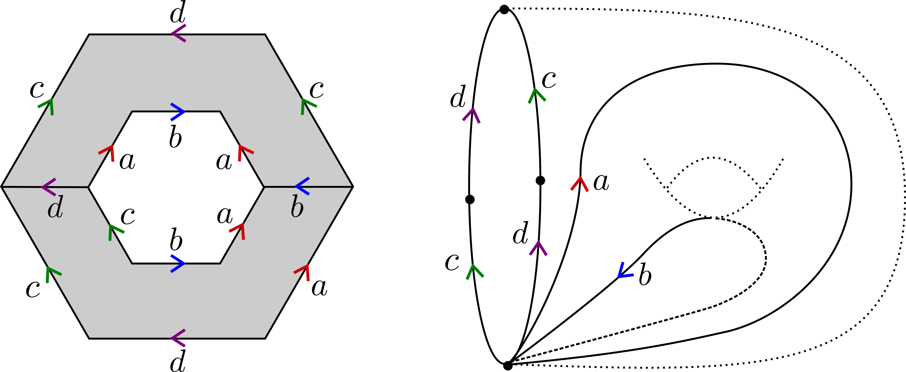
Consider the construction of the surface Σg\Sigma_{g} from a 4​g4g-gon by identifying its edges in pairs according to the pattern a1​b1​a1−1​b1−1​…​ag​bg​ag−1​bg−1a_{1}b_{1}a_{1}^{-1}b_{1}^{-1}\ldots a_{g}b_{g}a_{g}^{-1}b_{g}^{-1}. This gives rise to a CW-structure on Σg\Sigma_{g} consisting of one vertex (denoted oo), 2​g2g oriented 1−1-cells (denoted a1,b1,…,ag,bga_{1},b_{1},\ldots,a_{g},b_{g}) and one 22-cell which is the 4​g4g-gon glued along 4​g4g 11-cells88 8 We use the terms vertices and edges interchangeably with 00-cells and 11-cells, respectively.. See Figure 2.1 (in our running examples with g=2g=2, we denote the generators of Γ2\Gamma_{2} by a,b,c,da,b,c,d instead of a1,b1,a2,b2a_{1},b_{1},a_{2},b_{2}). We identify Γg\Gamma_{g} with π1​(Σg,o)\pi_{1}\left(\Sigma_{g},o\right), so that in the presentation (1.1), words in the generators a1,…,bga_{1},\ldots,b_{g} correspond to the homotopy class of the corresponding closed paths based at oo along the 11-skeleton of Σg\Sigma_{g}.

Refer to caption
Figure 2.1: The fixed CW-structure on Σ2\Sigma_{2}

Note that every covering space p:Υ→Σgp\colon\Upsilon\to\Sigma_{g} inherits a CW-structure from Σg\Sigma_{g}: the vertices are the pre-images of oo, and the open 11-cells (2-cells) are the connected components of the pre-images of the open 1-cells (2-cells, respectively) in Σg\Sigma_{g}. In particular, this is true for the universal covering space Σg~\widetilde{\Sigma_{g}}††margin: Σg~\widetilde{\Sigma_{g}} of Σg\Sigma_{g}, which we can now think of as a CW-complex. A sub-complex of a CW-complex is a subspace consisting of cells such that if some cell belongs to the subcomplex, then so are the cells of smaller dimension at its boundary.

Definition 2.1 (Tiled surface).

[MP21a, Definition 3.1] A tiled surface YY is a sub-complex of a (not-necessarily-connected) covering space of Σg\Sigma_{g}. In particular, a tiled surface is equipped with the restricted covering map p:Y→Σgp\colon Y\to\Sigma_{g} which is an immersion. We write 𝔳⁡(Y)\mathfrak{v}\left(Y\right) for the number of vertices of YY, 𝔢⁡(Y)\mathfrak{e}\left(Y\right) for the number of edges and 𝔣⁡(Y)\mathfrak{f}\left(Y\right)††margin: 𝔳⁡(Y),𝔢⁡(Y),𝔣⁡(Y){\scriptstyle\mathfrak{v}\left(Y\right),\mathfrak{e}\left(Y\right),\mathfrak{f}\left(Y\right)} for the number of 4​g4g-gons.

Alternatively, instead of considering a tiled surface YY to be a complex equipped with a restricted covering map, one may consider YY to be a complex as above with directed and labeled edges: the directions and labels (a1,b1,…,ag,bga_{1},b_{1},\ldots,a_{g},b_{g}) are pulled back from Σg\Sigma_{g} via pp. These labels uniquely determine pp as a combinatorial map between complexes. Figures 2.1 and 2.3 feature examples of tiled surfaces.

Note that a tiled surface is not always a surface: it may also contain vertices or edges with no 22-cells incident to them. However, as YY is a sub-complex of a covering space of Σg\Sigma_{g}, namely, of a surface, any neighborhood of YY inside the covering is a surface, and it is sometimes beneficial to think of YY as such.

Definition 2.2 (Thick version of a tiled surface).

[MP21a, Definition 3.2] Given a tiled surface YY which is a subcomplex of the covering space Υ\Upsilon of Σg\Sigma_{g}, adjoin to YY a small, closed, tubular neighborhood in Υ\Upsilon around every edge and a small closed disc in Υ\Upsilon around every vertex. The resulting closed surface, possibly with boundary, is referred to as the thick version of YY.

We let ∂Y\partial Y denote the boundary of the thick version of YY and 𝔡⁡(Y)\mathfrak{d}\left(Y\right)††margin: ∂Y,𝔡⁡(Y)\partial Y,\mathfrak{d}\left(Y\right) denote the number of edges along ∂Y\partial Y (so if an edge of YY does not border any 4​g4g-gon, it is counted twice).

In particular, 𝔡⁡(Y)=2​𝔢​(Y)−4​g​𝔣​(Y)\mathfrak{d}\left(Y\right)=2\mathfrak{e}\left(Y\right)-4g\mathfrak{f}\left(Y\right). We stress that we do not think of YY as a sub-complex, but rather as a complex for its own sake, which happens to have the capacity to be realized as a subcomplex of a covering space of Σg\Sigma_{g}. See [MP21a, Section 3] for a more detailed discussion.

It is occasionally useful, for example in Section 5, to augment the tiled surface YY by adding some new half-edges. Here, formally, a half-edge is a copy of the interval [0,12)[0,\frac{1}{2}) which is an (open) half of an edge of a covering space of Σg\Sigma_{g}.

Definition 2.3 (Tiled surface with hanging half-edges).

[MP21a, Section 3.2] Let YY be a tiled surface which is a subcomplex of the covering space p:Υ→Σgp\colon\Upsilon\to\Sigma_{g}. We denote by Y+Y_{+}††margin: Y+Y_{+} the tiled surface YY together with half edges of Υ\Upsilon which do not belong to YY but are incident to vertices of YY. Every half-edge of Y+Y_{+} added to YY in this manner is called a hanging half-edge. The thick version of Y+Y_{+} is, as above, Y+Y_{+} together with a small, closed, tubular neighborhood in Υ\Upsilon around every edge or hanging half-edge, and a small closed disc in Υ\Upsilon around every vertex. We denote by ∂Y+\partial Y_{+} the boundary of the think version of Y+Y_{+}.

Note that there are exactly 4​g4g half-edges incident to every vertex in Y+Y_{+}: some of them originate from edges in YY and some are hanging half-edges.

Morphisms of tiled surfaces

If Y1Y_{1} and Y2Y_{2} are tiled surfaces, a morphism from Y1Y_{1} to Y2Y_{2} is a map of C​WCW-complexes which maps ii-cells to ii-cells for i=0,1,2i=0,1,2 and respects the directions and labels of edges. Equivalently, this is a morphism of CW-complexes which commutes with the restricted covering maps pj:Yj→Σgp_{j}\colon Y_{j}\to\Sigma_{g} (j=1,2j=1,2). In particular, the restricted covering map from a tiled surface to Σg\Sigma_{g} is itself a morphism of tiled surfaces. It is an easy observation that every morphism of tiled surfaces is an immersion (locally injective).

2.1.2 Blocks and Chains

Some of the notions we use below are taken from [BS87]. See [MP21a, Section 3.2] for a more detailed account.

Given a covering space Υ\Upsilon of Σg\Sigma_{g}, every path in the 11-skeleton Υ(1)\Upsilon^{\left(1\right)} corresponds to a word in {a1±1,…,bg±1}\left\{a_{1}^{\pm 1},\ldots,b_{g}^{\pm 1}\right\}. A path that follows a (part of the) boundary of a 4​g4g-gon is called a block. If it has length at least 2​g+12g+1 it is called a long block, and if it has length exactly 2​g2g, it is called a half-block. If a (non-cyclic) block of length bb sits along the boundary of a 4​g4g-gon OO, the complement of the block is the block of length 4​g−b4g-b consisting of the complement set of edges along OO, so the block and its complement share the same starting point and the same terminal point.

A chain is a path in Υ(1)\Upsilon^{\left(1\right)} that consists of a sequence of blocks b1,…,brb_{1},\ldots,b_{r}, such that if the last vertex of bib_{i} and the first vertex of bi+1b_{i+1} is vv, there is exactly one edge incident to vv between the last edge of bib_{i} and the first edges of bi+1b_{i+1}. In other words, if the 4​g4g-gons corresponding to the blocks b1,…,brb_{1},\ldots,b_{r} are O1,…,OrO_{1},\ldots,O_{r}, then OiO_{i} and Oi+1O_{i+1} share an edge ee with an endpoint vv, and bib_{i} ends at vv and bi+1b_{i+1} starts at vv. See Figure 2.2. A long chain is a chain with corresponding blocks of lengths

2​g,2​g−1,2​g−1,…,2​g−1,2​g.2g,2g-1,2g-1,\ldots,2g-1,2g.

A half-chain is a cyclic chain (so the corresponding path is closed) consisting of blocks each of which is of length 2​g−12g-1. The complement of a long chain is the chain with blocks of lengths 2​g−1,2​g−1,…,2​g−12g-1,2g-1,\ldots,2g-1 which sits along the other side of the 4​g4g-gons bordering the long chain and with the same starting point and endpoint. Note that the complement of a long chain is shorter by two edges from the long chain (see Figure 2.2). The complement of a half-chain is defined as follows. If the half-chain sits along the boundary of the 4​g4g-gons O1,…,OrO_{1},\ldots,O_{r}, its complement is the half-chain sitting along the other sides of these 4​g4g-gons: a block (of length 2​g−12g-1) of the half-chain along OiO_{i} is replaced by the path of length 2​g−12g-1 along OiO_{i}, with starting and terminal points one edge away from the starting and terminal points, respectively, of the block. The complement of a half-chain has the same length as the original half-chain. The left part of Figure 2.3 illustrates two complementing half-chains of length 66 each (with two octagons in between).

Refer to caption
Figure 2.2: A long chain of total length 1717 (blocks of sizes 4,3,3,3,44,3,3,3,4, in blue) and its complement of length 1515 (in red)

A boundary cycle of YY is a cycle in Y(1)Y^{\left(1\right)} corresponding to an oriented boundary component of the thick version of YY (see Definition 2.2). We always choose the orientation so that there are no 4​g4g-gons to the immediate left of the boundary component as it is traversed. Therefore boundary components of YY correspond to unique cycles. Note that 𝔡⁡(Y)\mathfrak{d}\left(Y\right) is equal to the sum over boundary cycles of YY of the number of edges in each such cycle.

2.1.3 Boundary reduced and strongly boundary reduced tiled surfaces

The following definitions came up from our results in representation theory in §\lx@sectionsign5, but they fit perfectly with classical results in combinatorial group theory [Deh12] and in particular with [BS87].

Definition 2.4 (Boundary reduced).

A tiled surface YY is boundary reduced if no boundary cycle of YY contains a long block or a long chain.

In particular, if YY is boundary reduced, then every path that reads [a1,b1]​…​[ag,bg]\left[a_{1},b_{1}\right]\ldots\left[a_{g},b_{g}\right] is not only closed, but there is also a 4​g4g-gon attached to it. We also need a stronger version of this property.

Definition 2.5 (Strongly boundary reduced).

A tiled surface YY is strongly boundary reduced if no boundary cycle of YY contains a half-block or is a half-chain.

Because a long block contains (at least two) half-blocks and a long chain contains (two) half-blocks, a strongly boundary reduced tiled surface is in particular boundary reduced. The relevance of the notions of being (strongly) boundary reduced is that our techniques for estimating 𝔼nemb​(Y)\mathbb{E}_{n}^{\mathrm{emb}}\left(Y\right) for a tiled surface YY only give the right type of estimates when YY is boundary reduced – see Proposition 5.25. If YY is strongly boundary reduced we get even better estimates – see Proposition 5.26.

Let YY be a compact tiled surface which is a subcomplex of the covering space Υ\Upsilon of Σg\Sigma_{g}. In [MP21a, Section 4] we describe the “boundary reduced closure” 𝖡𝖱⁡(Y↪Υ)\mathsf{BR}\left(Y\hookrightarrow\Upsilon\right) of YY in Υ\Upsilon which is the smallest intermediate tiled surface which is boundary reduced. By (ibid, Proposition 4.6), 𝖡𝖱⁡(Y↪Υ)\mathsf{BR}\left(Y\hookrightarrow\Upsilon\right) is compact too. Likewise, 𝖲𝖡𝖱⁡(Y↪Υ)\mathsf{SBR}\left(Y\hookrightarrow\Upsilon\right), the strongly boundary reduced closure, is the smallest intermediate tiled surface which is strongly boundary reduced, but this one in not always compact. Our resolutions in Section 2.3 are based on a “compromise” between these two types of closures.

2.1.4 Core surfaces

Finally, let us define the main object which was introduced and analyzed in [MP21a], with motivation coming from the current paper. In analogy to Stallings core graphs and their role in the study of free groups and their subgroups, we introduced the notion of core surfaces which relates to subgroups of Γg\Gamma_{g}:

Definition 2.6 (Core surfaces).

[MP21a, Definition 1.1] Given a subgroup 1≠J≤Γg=π1​(Σg,o)1\neq J\leq\Gamma_{g}=\pi_{1}\left(\Sigma_{g},o\right), consider the covering space p:Υ→Σgp\colon\Upsilon\to\Sigma_{g} corresponding to JJ, so Υ=J\Σg~\Upsilon=J\backslash\widetilde{\Sigma_{g}}. Define the core surface of JJ, denoted Core⁡(J)\mathrm{Core}\left(J\right)††margin: Core⁡(J)\mathrm{Core}\left(J\right) , as the tiled surface which is a sub-complex of Υ\Upsilon as follows: (i)\left(i\right) take the union of all shortest-representative cycles in the 1-skeleton Υ(1)\Upsilon^{\left(1\right)} of every free-homotopy class of essential closed curve in Υ\Upsilon, and (i​i)\left(ii\right) add every connected component of the complement which contains finitely many 4​g4g-gons.

For completeness define the core surface of the trivial subgroup to be the 00-dimensional tiled surface consisting of a single vertex.

Note that the quotient Υ=J\Σg~\Upsilon=J\backslash\widetilde{\Sigma_{g}} is invariant under conjugation of JJ, so Core⁡(J)\mathrm{Core}\left(J\right) depends only on the conjugacy class of JJ in Γg\Gamma_{g}. Figure 2.3 gives two examples of core surfaces. As another example, if JJ is of finite index in Γ\Gamma, Core⁡(J)\mathrm{Core}\left(J\right) is identical to J\Σg~J\backslash\widetilde{\Sigma_{g}} and is a compact closed surface.

Refer to caption
Figure 2.3: Fix g=2g=2 and let Γ2=⟨a,b,c,d|[a,b][c,d]⟩\Gamma_{2}=\left\langle a,b,c,d\,\middle|\,\left[a,b\right]\left[c,d\right]\right\rangle. On the left is the core surface Core⁡(⟨a​b​a−2​b−1​c⟩)\mathrm{Core}\left(\left\langle aba^{-2}b^{-1}c\right\rangle\right). It consists of 1212 vertices, 1414 edges and two octagons, and topologically it is an annulus. On the right is the core surface Core⁡(⟨a,b⟩)\mathrm{Core}\left(\left\langle a,b\right\rangle\right). It consists of four vertices, six edges and one octagon, and topologically it is a genus-1 torus with one boundary component.

In [MP21a] we give an intrinsic definition of a core surface and show there is one-to-one correspondence between core surfaces (labeled by a1,…,bga_{1},\ldots,b_{g}) and conjugacy classes of subgroups of Γg\Gamma_{g}, we provide a “folding process” to construct Core⁡(J)\mathrm{Core}\left(J\right) from a finite generating set of JJ (provided, of course, that JJ is f.g.), and prove basic properties of core surfaces. In particular, Core⁡(J)\mathrm{Core}\left(J\right) is connected and strongly boundary reduced (ibid, Proposition 5.3), and whenever JJ is f.g., Core⁡(J)\mathrm{Core}\left(J\right) is compact (ibid, Proposition 5.8). We also show that whenever H≤J≤ΓgH\leq J\leq\Gamma_{g}, the natural morphism between the corresponding covering spaces H\Σg~→J\Σg~H\backslash\widetilde{\Sigma_{g}}\to J\backslash\widetilde{\Sigma_{g}}, restricts to a morphism Core⁡(H)→Core⁡(J)\mathrm{Core}\left(H\right)\to\mathrm{Core}\left(J\right).

2.2 Expectations and probabilities of tiled surfaces

Correspondence between Hom⁡(Γg,Sn)\mathrm{Hom}\left(\Gamma_{g},S_{n}\right) and nn-sheeted covering spaces of Σg\Sigma_{g}

Let MM be a connected topological space with basepoint mm. Consider nn-sheeted covering spaces of MM with the fiber above mm labeled by [n]\left[n\right], so that every point in the fiber has a different label. If MM is “nice enough”, in particular if MM is a surface, there is a one-to-one correspondence between these labeled nn-sheeted covering spaces and the set of homomorphisms Hom⁡(π1​(M,m),Sn)\mathrm{Hom}\left(\pi_{1}\left(M,m\right),S_{n}\right) (see, for instance, [Hat05, pages 68-70]). If M^\hat{M} is a labeled nn-sheeted covering space and p:M^→Mp\colon\hat{M}\to M the covering map, the corresponding homomorphism θ:π1​(M,m)→Sn\theta\colon\pi_{1}\left(M,m\right)\to S_{n} is given as follows: for h∈π1​(M,m)h\in\pi_{1}\left(M,m\right), consider γ\gamma, a closed path in MM, based at mm, which represents hh. Then θ​(h)​(i)=j\theta\left(h\right)\left(i\right)=j if and only if the lift of γ\gamma at the point ii ends at the point jj.99 9 There is a subtle issue here with the direction in which permutations are multiplied in SnS_{n}. The map θ:π1​(M,m)→Sn\theta\colon\pi_{1}\left(M,m\right)\to S_{n} as defined here is a homomorphism only if permutations in SnS_{n} are composed from right to left. We refer to this issue in the case of M=Σ2M=\Sigma_{2} in the beginning of Section 5.

In our case, this translates to a one-to-one correspondence between the representation space 𝕏g,n=Hom⁡(Γg,Sn)\mathbb{X}_{g,n}=\mathrm{Hom}\left(\Gamma_{g},S_{n}\right) and labeled nn-sheeted covering spaces of Σg\Sigma_{g} (pointed at oo). For ϕ:Γg→Sn\phi\colon\Gamma_{g}\to S_{n}, denote the corresponding covering space by pϕ:Xϕ→Σgp_{\phi}\colon X_{\phi}\to\Sigma_{g}. As explained above, XϕX_{\phi} inherits a CW-structure from Σg\Sigma_{g} and is, therefore, a tiled surface. The fiber above oo is precisely the vertices of XϕX_{\phi}, and they are labeled by [n]\left[n\right] in this construction.

Expected number of fixed points as expected number of lifts

Given a compact tiled surface YY, we are interested in the expected number of morphisms from YY to a random nn-covering of Σg\Sigma_{g}, namely, in

𝔼n(Y)=def𝔼ϕ∈𝕏g,n[#{morphismsY→Xϕ}],\mathbb{E}_{n}\left(Y\right)\stackrel{{\scriptstyle\mathrm{def}}}{{=}}\mathbb{E}_{\phi\in\mathbb{X}_{g,n}}\left[\#\left\{\mathrm{morphisms}~Y\to X_{\phi}\right\}\right],

where ϕ\phi is sampled uniformly at random from 𝕏g,n\mathbb{X}_{g,n}. Equivalently, this is the expected number of lifts of the restricted covering map p:Y→Σgp:Y\to\Sigma_{g} to the random nn-covering XϕX_{\phi}:

Xϕ\textstyle{X_{\phi}\ignorespaces\ignorespaces\ignorespaces\ignorespaces}pϕ\scriptstyle{p_{\phi}}Y\textstyle{Y\ignorespaces\ignorespaces\ignorespaces\ignorespaces\ignorespaces\ignorespaces\ignorespaces\ignorespaces}p\scriptstyle{p}Σg\textstyle{\Sigma_{g}}

Note that if YY is connected and ϕ∈𝕏g,n\phi\in\mathbb{X}_{g,n}, the number of morphisms Y→XϕY\to X_{\phi} is at most nn, as any vertex of YY can be lifted to one of the nn vertices of XϕX_{\phi}, and each such lift can be extended in at most one way to a lift of the whole of YY. For suitable choices of YY, 𝔼n​(Y)\mathbb{E}_{n}\left(Y\right) is equal to the quantities 𝔼g,n​[𝖿𝗂𝗑γ]\mathbb{E}_{g,n}\left[\mathsf{fix}_{\gamma}\right] and 𝔼g,n​[𝖿𝗂𝗑J]\mathbb{E}_{g,n}\left[\mathsf{fix}_{J}\right] that feature in our main theorems (Theorems 1.1, 1.2 and 1.3):

Lemma 2.7.

Let YY be a connected tiled surface and p:Y→Σgp\colon Y\to\Sigma_{g} the restricted covering map. For arbitrary vertex y∈Yy\in Y, assume that p∗​(π1​(Y,y))p_{*}\left(\pi_{1}\left(Y,y\right)\right) is conjugate to J≤f.g.ΓgJ\leq_{\mathrm{f.g.}}\Gamma_{g} (as a subgroup of π1​(Σg,o)=Γg\pi_{1}\left(\Sigma_{g},o\right)=\Gamma_{g}). Then for all n∈ℕn\in\mathbb{N},

𝔼n​(Y)=𝔼g,n​[𝖿𝗂𝗑J].\mathbb{E}_{n}\left(Y\right)=\mathbb{E}_{g,n}\left[\mathsf{fix}_{J}\right].

In particular, for J≤f.g.ΓgJ\leq_{\mathrm{f.g.}}\Gamma_{g},

𝔼n​(Core⁡(J))=𝔼g,n​[𝖿𝗂𝗑J].\mathbb{E}_{n}\left(\mathrm{Core}\left(J\right)\right)=\mathbb{E}_{g,n}\left[\mathsf{fix}_{J}\right].
Proof.

In fact, the equality holds at the level of the individual representation ϕ∈𝕏n=Hom⁡(Γg,Sn)\phi\in\mathbb{X}_{n}=\mathrm{Hom}\left(\Gamma_{g},S_{n}\right): the number of morphisms Y→XϕY\to X_{\phi} is equal to the number of common fixed points 𝖿𝗂𝗑J​(ϕ)\mathsf{fix}_{J}\left(\phi\right). Indeed, because the number of common fixed points of ϕ⁡(J)\phi\left(J\right) is the same as the number of fixed points of any conjugate, we may assume without loss of generality that p∗​(π1​(Y,y))=Jp_{*}\left(\pi_{1}\left(Y,y\right)\right)=J. Now, i∈[n]i\in\left[n\right] is a common fixed point of ϕ⁡(J)\phi\left(J\right) if and only if J≤π1​(Xϕ,vi)J\leq\pi_{1}\left(X_{\phi},v_{i}\right), where viv_{i} is the vertex of XϕX_{\phi} labeled ii, and π1​(Xϕ,vi)\pi_{1}\left(X_{\phi},v_{i}\right) is identified with the subgroup

(pϕ)∗​(π1​(Xϕ,vi))≤Γg.\left(p_{\phi}\right)_{*}\left(\pi_{1}\left(X_{\phi},v_{i}\right)\right)\leq\Gamma_{g}.

By standard facts from the theory of covering spaces [Hat05, Propositions 1.33 and 1.34], there is a lift of pp to XϕX_{\phi} mapping the vertex yy to viv_{i} if and only if (the image in Γg\Gamma_{g} of) π1​(Y,y)\pi_{1}\left(Y,y\right) is contained in (the image in Γg\Gamma_{g} of) π1​(Xϕ,vi)\pi_{1}\left(X_{\phi},v_{i}\right), and this lift, if exists, is unique.

The statement about core surfaces follows from the fact that (the image in Γg\Gamma_{g} of) π1​(Core​(J))\pi_{1}\left(\mathrm{Core}\left(J\right)\right) is conjugate to JJ [MP21a, Proposition 5.3]. ∎

Another type of expectation will also feature in this work. Given a compact tiled surface YY, denote

𝔼nemb(Y)=def𝔼ϕ∈𝕏g,n[#{injectivemorphismsY→Xϕ}],\mathbb{E}_{n}^{\mathrm{emb}}\left(Y\right)\stackrel{{\scriptstyle\mathrm{def}}}{{=}}\mathbb{E}_{\phi\in\mathbb{X}_{g,n}}\left[\#\left\{\mathrm{injective~morphisms}~Y\to X_{\phi}\right\}\right],

where the expectation is over a uniformly random ϕ∈𝕏g,n\phi\in\mathbb{X}_{g,n}.

2.3 Resolutions

Definition 2.8 (Resolutions).

A resolution ℛ\mathcal{\mathcal{R}} of a tiled surface YY is a collection of morphisms of tiled surfaces

ℛ={f:Y→Wf},\mathcal{R}=\left\{f\colon Y\to W_{f}\right\},

such that every morphism h:Y→Zh\colon Y\to Z of YY into a tiled surface ZZ with no boundary decomposes uniquely as Y→fWf↪h¯ZY\stackrel{{\scriptstyle f}}{{\to}}W_{f}\stackrel{{\scriptstyle\overline{h}}}{{\hookrightarrow}}Z, where f∈ℛf\in\mathcal{R} and h¯\overline{h} is an embedding.

The purpose of introducing resolutions is the following obvious lemma. Recall the notation 𝔼n​(Y)\mathbb{E}_{n}\left(Y\right) and 𝔼nemb​(Y)\mathbb{E}_{n}^{\mathrm{emb}}\left(Y\right) from Section 2.2.

Lemma 2.9.

If YY is a compact tiled surface and ℛ\mathcal{R} is a finite resolution of YY, then

𝔼n​(Y)=∑f∈ℛ𝔼nemb​(Wf).\mathbb{E}_{n}\left(Y\right)=\sum_{f\in\mathcal{R}}\mathbb{E}_{n}^{\mathrm{emb}}\left(W_{f}\right). (2.1)

Our main goal in the rest of this subsection is to prove the existence of a finite resolution whenever we are given a compact tiled surface YY – this is the content of Theorem 2.14 below. This resolution will consist strictly of boundary reduced tiled surfaces WfW_{f}, and some of these will even be strongly boundary reduced. We shall make use of Theorem 2.14 mainly for YY a core surface of a finitely generated subgroup of Γ\Gamma. In this case the resolution we construct has even nicer properties – see Proposition 2.15.

Ideally, we would have liked to get a resolution where all the elements are strongly boundary reduced. Unfortunately, such a resolution does not always exist. For example, when g=2g=2 and Γ2=⟨a,b,c,d|[a,b][c,d]⟩\Gamma_{2}=\left\langle a,b,c,d\,\middle|\,\left[a,b\right]\left[c,d\right]\right\rangle, the core surface Y=Core⁡(⟨[a,b]⟩)Y=\mathrm{Core}\left(\left\langle\left[a,b\right]\right\rangle\right) does not admit such a resolution as can be inferred from [MP21a, Figure 4.2].

To prove the existence of a resolution with nice properties, we first define a process which outputs a “compromise” between the 𝖡𝖱\mathsf{BR}-closure of a tiled surface and the 𝖲𝖡𝖱\mathsf{SBR}-closure, introduced in [MP21a, Section 4].

Definition 2.10.

Fix χ0∈ℤ\chi_{0}\in\mathbb{Z}. Assume that h:Y→Zh\colon Y\to Z is a morphism between tiled surfaces where YY is compact and ZZ has no boundary. Let W0W_{0} denote the hh-image of YY in ZZ. Set i=0i=0. Perform the following algorithm we call the growing process:

  1. 1.

    If one of the following conditions holds:

    1. (a)

      WiW_{i} is strongly boundary reduced, or

    2. (b)

      WiW_{i} is boundary reduced and χ⁡(Wi)<χ0\chi\left(W_{i}\right)<\chi_{0},

    terminate and return h:Y→Wih\colon Y\to W_{i}.

  2. 2.

    Obtain Wi+1W_{i+1} from WiW_{i} by adding to WiW_{i} (the closure of) every 4​g4g-gon in Z∖WiZ\setminus W_{i} which touches along its boundary an edge of ∂Wi\partial W_{i} which is part of a half-block (this includes the case of a long block), a long chain or a half-chain. Set i:=i+1i:=i+1 and return to item 11.

It is clear that every step of this process is deterministic. Note that if the process ends when WiW_{i} is strongly boundary reduced, then WiW_{i} is the unique smallest strongly boundary reduced tiled surface inside ZZ containing W0W_{0}, denoted 𝖲𝖡𝖱⁡(Y↪Z)\mathsf{SBR}(Y\hookrightarrow Z) [MP21a, Section 4]. (In general, 𝖲𝖡𝖱⁡(Y↪Z)\mathsf{SBR}(Y\hookrightarrow Z) is not always compact, but in this case it is.) The growing process always terminates after finitely many steps:

Lemma 2.11.

The process described in Definition 2.10 always terminates.

Proof.

Let 𝔥​𝔢​(Wi)\mathfrak{he}\left(W_{i}\right) denote the number of hanging half-edges along the boundary of (Wi)+\left(W_{i}\right)_{+} and consider the triple

(𝔡⁡(Wi),χ⁡(Wi),−𝔥​𝔢​(Wi)).\left(\mathfrak{d}\left(W_{i}\right),\chi\left(W_{i}\right),-\mathfrak{he}\left(W_{i}\right)\right). (2.2)

For every ii, WiW_{i} is a compact sub-surface of ZZ, and so the three quantities are well-defined integers. We claim that at every step in the growing process, the triple (2.2) strictly reduces with respect to the lexicographic order.

Indeed, assume we do not halt after ii steps, and let O1,…,OkO_{1},\ldots,O_{k} be the list of 4​g4g-gons in Z∖WiZ\setminus W_{i} which are added to WiW_{i} in order to obtain Wi+1W_{i+1}. By the choice of 4​g4g-gons, it is clear that 𝔡⁡(Wi+1)≤𝔡⁡(Wi)\mathfrak{d}\left(W_{i+1}\right)\leq\mathfrak{d}\left(W_{i}\right). If the inequality is strict, we are done. So assume 𝔡⁡(Wi+1)=𝔡⁡(Wi)\mathfrak{d}\left(W_{i+1}\right)=\mathfrak{d}\left(W_{i}\right). This means that ∂(Wi)\partial\left(W_{i}\right) contains no long blocks nor long chains, so it is boundary reduced, and that the edges in the complements in ZZ of the half-blocks and half-chains at ∂(Wi)\partial\left(W_{i}\right) all belong to ∂(Wi+1)\partial\left(W_{i+1}\right). In other words, let p1,…,pmp_{1},\ldots,p_{m} be these complements in ZZ: so pjp_{j} is either a half-block or a half-chain. The equality 𝔡⁡(Wi+1)=𝔡⁡(Wi)\mathfrak{d}\left(W_{i+1}\right)=\mathfrak{d}\left(W_{i}\right) means that all the edges in p1,…,pmp_{1},\ldots,p_{m} belong to ∂Wi+1\partial W_{i+1}.

It is easy to see that in this case χ⁡(Wi+1)≤χ⁡(Wi)\chi\left(W_{i+1}\right)\leq\chi\left(W_{i}\right): the number of new 4​g4g-gons and vertices in Wi+1W_{i+1} at most balances the number of new edges. Let VV denote the set of internal vertices in p1,…,pmp_{1},\ldots,p_{m} (so not at their endpoints). We have strict inequality χ⁡(Wi+1)<χ⁡(Wi)\chi\left(W_{i+1}\right)<\chi\left(W_{i}\right) if and only if some v∈Vv\in V belongs to WiW_{i} or to two different complements from p1,…,pmp_{1},\ldots,p_{m}.

Now assume that 𝔡⁡(Wi+1)=𝔡⁡(Wi)\mathfrak{d}\left(W_{i+1}\right)=\mathfrak{d}\left(W_{i}\right) and χ⁡(Wi+1)=χ⁡(Wi)\chi\left(W_{i+1}\right)=\chi\left(W_{i}\right). Then WiW_{i} is boundary reduced and each of the complements p1,…,pmp_{1},\ldots,p_{m} is a connected piece of ∂Wi+1\partial W_{i+1}. If OjO_{j} touches a half-block of ∂Wi\partial W_{i}, its annexation adds a net of (2​g−1)​(4​g−2)−2=8​g​(g−1)\left(2g-1\right)\left(4g-2\right)-2=8g\left(g-1\right) hanging half-edges. Every 4​g4g-gon along a half-chain of ∂Wi\partial W_{i} also adds on average a net of 8​g​(g−1)8g\left(g-1\right) hanging half-edges. So if we add at least one 4​g4g-gon at the (i+1)\left(i+1\right)st step, −𝔥​𝔢-\mathfrak{he} strictly decreases. So indeed the triple (2.2) strictly decreases lexicographically in every step.

Finally, there are at most finitely many steps in which 𝔡⁡(Wi)\mathfrak{d}\left(W_{i}\right) decreases, because this is a non-negative integer. So it is enough to show there cannot be infinitely many steps in which 𝔡⁡(Wi)\mathfrak{d}\left(W_{i}\right) is constant. If 𝔡⁡(Wi+1)=𝔡⁡(Wi)\mathfrak{d}\left(W_{i+1}\right)=\mathfrak{d}\left(W_{i}\right), then WiW_{i} is boundary reduced. If χ⁡(Wi)\chi\left(W_{i}\right) keeps decreasing, then eventually we hit the bound χ⁡(Wi)<χ0\chi\left(W_{i}\right)<\chi_{0} and halt. If 𝔡⁡(Wi)\mathfrak{d}\left(W_{i}\right) and χ⁡(Wi)\chi\left(W_{i}\right) are constant, then 𝔥​𝔢​(Wi)\mathfrak{he}\left(W_{i}\right) increases constantly, but in every tiled surface WW, 𝔥​𝔢​(W)≤4​g​𝔡​(W)\mathfrak{he}\left(W\right)\leq 4g\mathfrak{d}\left(W\right), so there cannot be infinitely many steps of this type too. This proves the lemma. ∎

Lemma 2.12.

There is a bound B=B⁡(Y)B=B\left(Y\right), independent of h:Y→Zh\colon Y\to Z, such that in the entire growing process, at most B=B⁡(Y)B=B\left(Y\right) 4​g4g-gons are added to W0W_{0}.

Proof.

Note that every boundary edge of W0W_{0} is necessarily an hh-image of a boundary edge of YY, so that 𝔡⁡(Wi)≤𝔡⁡(W0)≤𝔡⁡(Y)\mathfrak{d}\left(W_{i}\right)\leq\mathfrak{d}\left(W_{0}\right)\leq\mathfrak{d}\left(Y\right). In every step, we add at most 𝔡⁡(Wi)2​g−1≤𝔡⁡(Y)2​g−1\frac{\mathfrak{d}\left(W_{i}\right)}{2g-1}\leq\frac{\mathfrak{d}\left(Y\right)}{2g-1} 4​g4g-gons. So it is enough to bound the number of steps performed in the growing process until it terminates. There are at most 𝔡⁡(Y)2\frac{\mathfrak{d}\left(Y\right)}{2} steps in which 𝔡⁡(Wi)\mathfrak{d}\left(W_{i}\right) strictly decreases (𝔡⁡(Wi+1)<𝔡⁡(Wi)\mathfrak{d}\left(W_{i+1}\right)<\mathfrak{d}\left(W_{i}\right)), so there are at most 𝔡⁡(Y)2+1\frac{\mathfrak{d}\left(Y\right)}{2}+1 possible values of 𝔡⁡(Wi)\mathfrak{d}\left(W_{i}\right). In steps where 𝔡⁡(Wi)\mathfrak{d}\left(W_{i}\right) is unchanged, WiW_{i} is boundary reduced, so by definition χ⁡(Wi)≥χ0\chi\left(W_{i}\right)\geq\chi_{0} (otherwise, the process terminates). Let π0​(Y)\pi_{0}\left(Y\right) denote the number of connected components of YY. For all ii, WiW_{i} is a sub-surface of ZZ with at most π0​(Y)\pi_{0}\left(Y\right) connected components, and by the classification of surfaces, χ⁡(Wi)≤2​π0​(Y)\chi\left(W_{i}\right)\leq 2\pi_{0}\left(Y\right). There are at most 2​π0​(Y)−χ02\pi_{0}\left(Y\right)-\chi_{0} steps with 𝔡⁡(Wi)\mathfrak{d}\left(W_{i}\right) fixed and χ⁡(Wi)\chi\left(W_{i}\right) strictly decreasing. Finally, when 𝔡⁡(Wi)\mathfrak{d}\left(W_{i}\right) is constant there are at most 2​π0​(Y)−χ0+12\pi_{0}\left(Y\right)-\chi_{0}+1 possible values of χ⁡(Wi)\chi\left(W_{i}\right), and if 𝔡⁡(Wi+1)=𝔡⁡(Wi)\mathfrak{d}\left(W_{i+1}\right)=\mathfrak{d}\left(W_{i}\right) and χ⁡(Wi+1)=χ⁡(Wi)\chi\left(W_{i+1}\right)=\chi\left(W_{i}\right) then 𝔥​𝔢​(Wi+1)≥𝔥​𝔢​(Wi)+8​g​(g−1)\mathfrak{he}\left(W_{i+1}\right)\geq\mathfrak{he}\left(W_{i}\right)+8g\left(g-1\right) and 𝔥​𝔢​(Wi)≤4​g​𝔡​(Wi)≤4​g​𝔡​(Y)\mathfrak{he}\left(W_{i}\right)\leq 4g\mathfrak{d}\left(W_{i}\right)\leq 4g\mathfrak{d}\left(Y\right), so there are at most 𝔡⁡(Y)2​(g−1)\frac{\mathfrak{d}\left(Y\right)}{2\left(g-1\right)} steps with the same value of 𝔡⁡(Wi)\mathfrak{d}\left(W_{i}\right) and χ⁡(Wi)\chi\left(W_{i}\right). Overall there are at most

𝔡⁡(Y)2+(𝔡⁡(Y)2+1)​[(2​π0​(Y)−χ0)+(2​π0​(Y)−χ0+1)⋅𝔡⁡(Y)2​(g−1)]\frac{\mathfrak{d}\left(Y\right)}{2}+\left(\frac{\mathfrak{d}\left(Y\right)}{2}+1\right)\left[\left(2\pi_{0}\left(Y\right)-\chi_{0}\right)+\left(2\pi_{0}\left(Y\right)-\chi_{0}+1\right)\cdot\frac{\mathfrak{d}\left(Y\right)}{2\left(g-1\right)}\right] (2.3)

steps in the growing process. Define B⁡(Y)B\left(Y\right) to be 𝔡⁡(Y)2​g−1\frac{\mathfrak{d}\left(Y\right)}{2g-1} times (2.3). ∎

We can now define the sought-after resolution for compact tiled surfaces.

Definition 2.13.

Suppose that YY is a compact tiled surface and χ0∈ℤ\chi_{0}\in\mathbb{Z} a fixed integer. Define the χ0\chi_{0}-resolution of YY to be the collection

ℛ=ℛ⁡(Y,χ0)={f:Y→Wf}\mathcal{R}=\mathcal{R}\left(Y,\chi_{0}\right)=\left\{f\colon Y\to W_{f}\right\}

obtained from all possible morphisms h:Y→Zh\colon Y\to Z from YY to a tiled surface ZZ with no boundary via the growing process (the process applied with parameter χ0\chi_{0}).

Theorem 2.14.

Suppose YY is a compact tiled surface and χ0∈ℤ\chi_{0}\in\mathbb{Z} a fixed integer. The collection ℛ=ℛ⁡(Y,χ0)\mathcal{R}=\mathcal{R}\left(Y,\chi_{0}\right) from Definition 2.13 is a finite resolution of YY which satisfies further

R1

for every f∈ℛf\in\mathcal{R}, the tiled surface WfW_{f} is compact and boundary reduced, and

R2

for every f∈ℛf\in\mathcal{R} with χ⁡(Wf)≥χ0\chi\left(W_{f}\right)\geq\chi_{0}, the tiled surface WfW_{f} is strongly boundary reduced.

Proof.

By Lemma 2.11 and the halting conditions of the growing process, it is clear that every such morphism in ℛ\mathcal{R} satisfies R1 and R2. Given a morphism h:Y→Zh\colon Y\to Z as in Definition 2.13, h⁡(Y)h\left(Y\right) (also named W0W_{0}) is a quotient of YY and therefore the number of cells in h⁡(Y)h\left(Y\right) is bounded. From Lemma 2.12 we now conclude that that there is a bound on the number of cells in any WfW_{f} with f∈ℛf\in\mathcal{R}. This shows that ℛ\mathcal{R} is finite as there are finitely many tiled surfaces with given bounds on the number of cells, and finitely many morphisms between two given compact tiled surfaces.

It remains to show that ℛ\mathcal{R} is a resolution. By the way it was constructed, it is clear that every morphism h:Y→Zh\colon Y\to Z with ∂Z=∅\partial Z=\emptyset, decomposes as

Y→fWf↪ZY\stackrel{{\scriptstyle f}}{{\to}}W_{f}\hookrightarrow Z (2.4)

and that f∈ℛf\in\mathcal{R}. To show uniqueness, assume that hh decomposes in an additional way

Y→φWφ↪ZY\stackrel{{\scriptstyle\varphi}}{{\to}}W_{\varphi}\hookrightarrow Z (2.5)

where WφW_{\varphi} is the result of the growing process for some h′:Y→Z′h^{\prime}\colon Y\to Z^{\prime} with ∂Z′=∅\partial Z^{\prime}=\emptyset. We claim that (2.4) and (2.5) are precisely the same decompositions of hh. Indeed, the growing process defined by h′:Y→Z′h^{\prime}\colon Y\to Z^{\prime} takes place entirely inside WφW_{\varphi}, and does not depend on the structure of Z′\WφZ^{\prime}\backslash W_{\varphi}: in the (i+1)\left(i+1\right)st step of the growing process, the decision whether or not to annex more 4​g4g-gons and where, depends only on the structure and boundary of WiW_{i}. Consequently, the growing process defined by the morphism h′:Y→Z′h^{\prime}\colon Y\to Z^{\prime} has the exact same output, in terms of the resulting element we add to ℛ\mathcal{R}, as the growing process defined by the composition Y→φWφ↪ZY\stackrel{{\scriptstyle\varphi}}{{\to}}W_{\varphi}\hookrightarrow Z. But because the growing process is deterministic, the latter is identical to the growing process defined by h:Y→Zh\colon Y\to Z. ∎

As mentioned above, we will use Theorem 2.14 mainly with YY being a core surface. In this case, the theorem can be strengthened as follows. Recall from Section 1 that given J≤f.g.ΓgJ\leq_{\mathrm{f.g.}}\Gamma_{g}, we denote by 𝔐​𝔒​𝔊​(J)\mathfrak{MOG}\left(J\right) the set of f.g. overgroups of JJ with maximal Euler characteristic, and by χmax​(J)\chi_{\max}\left(J\right) this maximal Euler characteristic.

Proposition 2.15 (Addendum to Theorem 2.14).

Let J≤f.g.ΓgJ\leq_{\mathrm{f.g.}}\Gamma_{g} and let χ0∈ℤ\chi_{0}\in\mathbb{Z}. Let ℛJ,χ0={f:Core⁡(J)→Wf}\mathcal{R}_{J,\chi_{0}}=\left\{f\colon\mathrm{Core}\left(J\right)\to W_{f}\right\} be the resolution ℛ⁡(Core⁡(J),χ0)\mathcal{R}\left(\mathrm{Core}\left(J\right),\chi_{0}\right) from Definition 2.13. Then ℛJ,χ0\mathcal{R}_{J,\chi_{0}} satisfies further the following two properties.

R3

For every f∈ℛJ,χ0f\in\mathcal{R}_{J,\chi_{0}} with χ⁡(Wf)≥χ0\chi\left(W_{f}\right)\geq\chi_{0}, the tiled surface WfW_{f} is the core surface of some K≤f.g.ΓgK\leq_{\mathrm{f.g.}}\Gamma_{g} with J≤KJ\leq K and ff is the natural morphism between the two core surfaces (the restriction of J\Σg~→K\Σg~J\backslash\widetilde{\Sigma_{g}}\to K\backslash\widetilde{\Sigma_{g}}).

R4

Assume that χ0≤χmax​(J)\chi_{0}\leq\chi_{\max}\left(J\right). Then for every K∈𝔐​𝔒​𝔊​(J)K\in\mathfrak{MOG}\left(J\right), the natural morphism Core⁡(J)→Core⁡(K)\mathrm{Core}\left(J\right)\to\mathrm{Core}\left(K\right) belongs to ℛJ,χ0\mathcal{R}_{J,\chi_{0}}.

For K≤f.g.ΓgK\leq_{\mathrm{f.g.}}\Gamma_{g} we have χ⁡(K)=χ⁡(Core⁡(K))\chi\left(K\right)=\chi\left(\mathrm{Core}\left(K\right)\right) [MP21a, Proposition 5.3]. Proposition 2.15 thus shows that as long as χ0≤χmax​(J)\chi_{0}\leq\chi_{\max}\left(J\right), there is a bijection between the elements of 𝔐​𝔒​𝔊​(J)\mathfrak{MOG}\left(J\right) and the elements in the resolution with maximal Euler characteristic.

Corollary 2.16.

For every J≤f.g.ΓgJ\leq_{\mathrm{f.g.}}\Gamma_{g}, the set 𝔐​𝔒​𝔊​(J)\mathfrak{MOG}\left(J\right) of f.g. overgroups of maximal Euler characteristic is finite.

Proof of Proposition 2.15.

Suppose that f:Core⁡(J)→Wff\colon\mathrm{Core}\left(J\right)\to W_{f} satisfies χ⁡(Wf)≥χ0\chi\left(W_{f}\right)\geq\chi_{0}. In particular, WfW_{f} is strongly boundary reduced by R2. Let j∈Core⁡(J)j\in\mathrm{Core}\left(J\right) be a vertex and assume without loss of generality that J=π1​(Core⁡(J),j)J=\pi_{1}\left(\mathrm{Core}\left(J\right),j\right) (recall that if (Y,y0)\left(Y,y_{0}\right) is a based tiled surface, we identify π1​(Y,y0)\pi_{1}\left(Y,y_{0}\right) with the subgroup p∗​(π1​(Y,y0))p_{*}\left(\pi_{1}\left(Y,y_{0}\right)\right) of π1​(Σg,o)=Γg\pi_{1}\left(\Sigma_{g},o\right)=\Gamma_{g}). Define K=defπ1​(Wf,f⁡(j))K\stackrel{{\scriptstyle\mathrm{def}}}{{=}}\pi_{1}\left(W_{f},f\left(j\right)\right). As WfW_{f} is compact, KK is finitely generated. Let pK:(K\Σg~,k)→Σgp_{K}\colon\left(K\backslash\widetilde{\Sigma_{g}},k\right)\to\Sigma_{g} be the pointed coverings space with π1​(K\Σg~,k)=K\pi_{1}\left(K\backslash\widetilde{\Sigma_{g}},k\right)=K. By the unique lifting property from the theory of covering spaces [Hat05, Propositions 1.33 and 1.34], as WfW_{f} is connected, there is a unique lift α\alpha of the restricted covering map pWf:Wf→Σgp_{W_{f}}\colon W_{f}\to\Sigma_{g} to K\Σg~K\backslash\widetilde{\Sigma_{g}}, which maps f⁡(j)f\left(j\right) to kk. We will show that α\alpha gives an isomorphism between WfW_{f} and Core⁡(K)\mathrm{Core}\left(K\right).

(Core⁡(K),k)\textstyle{\left(\mathrm{Core}\left(K\right),k\right)\ignorespaces\ignorespaces\ignorespaces\ignorespaces}ι\scriptstyle{\iota}(K\Σg~,k)\textstyle{\left(K\backslash\widetilde{\Sigma_{g}},k\right)\ignorespaces\ignorespaces\ignorespaces\ignorespaces}pK\scriptstyle{p_{K}}(Core⁡(K),k)\textstyle{\left(\mathrm{Core}\left(K\right),k\right)\ignorespaces\ignorespaces\ignorespaces\ignorespaces}ι\scriptstyle{\iota}(K\Σg~,k)\textstyle{\left(K\backslash\widetilde{\Sigma_{g}},k\right)\ignorespaces\ignorespaces\ignorespaces\ignorespaces}m\scriptstyle{m}(Core⁡(J),j)\textstyle{\left(\mathrm{Core}\left(J\right),j\right)\ignorespaces\ignorespaces\ignorespaces\ignorespaces\ignorespaces\ignorespaces\ignorespaces\ignorespaces}f\scriptstyle{f}(Wf,f⁡(j))\textstyle{\left(W_{f},f\left(j\right)\right)\ignorespaces\ignorespaces\ignorespaces\ignorespaces\ignorespaces\ignorespaces\ignorespaces\ignorespaces}pWf\scriptstyle{p_{W_{f}}}∃!α\scriptstyle{\exists!\alpha}(Σg,o)\textstyle{\left(\Sigma_{g},o\right)}(Wf,f⁡(j))\textstyle{\left(W_{f},f\left(j\right)\right)\ignorespaces\ignorespaces\ignorespaces\ignorespaces}(Z,f⁡(j))\textstyle{\left(Z,f\left(j\right)\right)}

First we show that α⁡(Wf)⊆Core⁡(K)\alpha\left(W_{f}\right)\subseteq\mathrm{Core}\left(K\right). Recall that WfW_{f} is the result of the growing process for some h:Core⁡(J)→Zh\colon\mathrm{Core}\left(J\right)\to Z with ∂Z=∅\partial Z=\emptyset. Consider W0=defh⁡(Core⁡(J))⊆ZW_{0}\stackrel{{\scriptstyle\mathrm{def}}}{{=}}h\left(\mathrm{Core}\left(J\right)\right)\subseteq Z. Recall that Wf=𝖲𝖡𝖱⁡(W0↪Z)W_{f}=\mathsf{SBR}\left(W_{0}\hookrightarrow Z\right). By the unique lifting property, α∘f\alpha\circ f is the natural morphism Core⁡(J)→K\Σg~\mathrm{Core}\left(J\right)\to K\backslash\widetilde{\Sigma_{g}}, which, by [MP21a, Lemma 5.4], has image contained in Core⁡(K)\mathrm{Core}\left(K\right). Hence α⁡(W0)⊆Core⁡(K)\alpha\left(W_{0}\right)\subseteq\mathrm{Core}\left(K\right). As Core⁡(K)\mathrm{Core}\left(K\right) is strongly boundary reduced [MP21a, Propositions 5.3], we have that 𝖲𝖡𝖱⁡(α⁡(W0)↪K\Σg~)\mathsf{SBR}\left(\alpha\left(W_{0}\right)\hookrightarrow K\backslash\widetilde{\Sigma_{g}}\right) is contained in Core⁡(K)\mathrm{Core}\left(K\right). By [MP21a, Lemma 4.7],

α⁡(Wf)=α⁡(𝖲𝖡𝖱⁡(W0↪Z))⊆𝖲𝖡𝖱⁡(α⁡(W0)↪K\Σg~)⊆Core⁡(K).\alpha\left(W_{f}\right)=\alpha\left(\mathsf{SBR}\left(W_{0}\hookrightarrow Z\right)\right)\subseteq\mathsf{SBR}\left(\alpha\left(W_{0}\right)\hookrightarrow K\backslash\widetilde{\Sigma_{g}}\right)\subseteq\mathrm{Core}\left(K\right).

Now ZZ is a covering space of Σg\Sigma_{g} and we may assume it is connected (because Core⁡(J)\mathrm{Core}\left(J\right) is). Thus ZZ is identical to L\Σg~L\backslash\widetilde{\Sigma_{g}} for some L=π1​(Z,h​(j))L=\pi_{1}\left(Z,h\left(j\right)\right). By property R2, WfW_{f} is strongly boundary reduced, and so by [MP21a, Corollary 4.11] its embedding in ZZ is π1\pi_{1}-injective. In other words, K≤LK\leq L, and, therefore, there is a morphism m:(K\Σg~,k)→(Z,f⁡(j))m\colon\left(K\backslash\widetilde{\Sigma_{g}},k\right)\to\left(Z,f\left(j\right)\right). By the unique lifting property, the composition m∘α:(Wf,f⁡(j))→(Z,f⁡(j))m\circ\alpha\colon\left(W_{f},f\left(j\right)\right)\to\left(Z,f\left(j\right)\right) must be identical to the embedding (Wf,f⁡(j))↪(Z,f⁡(j))\left(W_{f},f\left(j\right)\right)\hookrightarrow\left(Z,f\left(j\right)\right) and therefore α\alpha is injective. So α⁡(Wf)\alpha\left(W_{f}\right) is a strongly boundary reduced sub-surface of Core⁡(K)\mathrm{Core}\left(K\right) with fundamental group KK. By [MP21a, Lemma 5.7] if follows that α⁡(Wf)⊇Core⁡(K)\alpha\left(W_{f}\right)\supseteq\mathrm{Core}\left(K\right). We conclude that α:Wf→Core⁡(K)\alpha\colon W_{f}\to\mathrm{Core}\left(K\right) is an isomorphism, and R3 is proven.

To prove R4, suppose that K∈𝔐​𝔒​𝔊​(J)K\in\mathfrak{MOG}\left(J\right). Let h:Core⁡(J)→K\Σg~h\colon\mathrm{Core}\left(J\right)\to K\backslash\widetilde{\Sigma_{g}} be the natural morphism. By the definition of the resolution ℛJ\mathcal{R}_{J}, the morphism hh factors as Core⁡(J)→fWf↪K\Σg~\mathrm{Core}\left(J\right)\stackrel{{\scriptstyle f}}{{\to}}W_{f}\stackrel{{\scriptstyle}}{{\hookrightarrow}}K\backslash\widetilde{\Sigma_{g}} for some f∈ℛJf\in\mathcal{R}_{J}. Because h⁡(Core⁡(J))⊆Core⁡(K)h\left(\mathrm{Core}\left(J\right)\right)\subseteq\mathrm{Core}\left(K\right) (by [MP21a, Lemma 5.4]), and because Core⁡(K)\mathrm{Core}\left(K\right) is strongly boundary reduced, we have Wf⊆Core⁡(K)W_{f}\subseteq\mathrm{Core}\left(K\right).

Let CC be a connected component of the difference between the thick version of Core⁡(K)\mathrm{Core}\left(K\right) and the thick version of WfW_{f}. As Core⁡(K)\mathrm{Core}\left(K\right) is compact, C¯\overline{C} is compact. As Core⁡(K)\mathrm{Core}\left(K\right) is connected, C¯\overline{C} must intersect ∂Wf\partial W_{f} and in particular has at least one boundary component. As WfW_{f} is boundary reduced, C¯\overline{C} is not homeomorphic to a disc, and so χ⁡(C¯)≤0\chi\left(\overline{C}\right)\leq 0. Now

χ⁡(K)=χ⁡(Core⁡(K))=χ⁡(Wf)+∑Cχ⁡(C¯),\chi\left(K\right)=\chi\left(\mathrm{Core}\left(K\right)\right)=\chi\left(W_{f}\right)+\sum_{C}\chi\left(\overline{C}\right),

the sum being over all connected components as above. We conclude that χ⁡(Wf)≥χ⁡(K)=χmax​(J)≥χ0\chi\left(W_{f}\right)\geq\chi\left(K\right)=\chi_{\max}\left(J\right)\geq\chi_{0}. By R2, WfW_{f} is strongly boundary reduced and by R3, Wf=Core⁡(M)W_{f}=\mathrm{Core}\left(M\right) for some subgroup MM. But then M∈𝔐​𝔒​𝔊​(J)M\in\mathfrak{MOG}\left(J\right), χ⁡(Core⁡(M))=χ⁡(K)\chi\left(\mathrm{Core}\left(M\right)\right)=\chi\left(K\right), and every connected component CC as above satisfies χ⁡(C¯)=0\chi\left(\overline{C}\right)=0. As C¯\overline{C} has at least one boundary component, it must be an annulus. But then Core⁡(M)\mathrm{Core}\left(M\right) is a deformation retract of Core⁡(K)\mathrm{Core}\left(K\right), so M=KM=K up to conjugation and so Wf=Core⁡(M)=Core⁡(K)W_{f}=\mathrm{Core}\left(M\right)=\mathrm{Core}\left(K\right). ∎

Corollary 2.17.

Suppose 1≠γ∈Γg1\neq\gamma\in\Gamma_{g} is a non-trivial element. Let qq be the maximal natural number such that γ=γ0q\gamma=\gamma_{0}^{~q} for some γ0∈Γg\gamma_{0}\in\Gamma_{g}, and d⁡(q)d(q) the number of positive divisors of qq. Then Core⁡(⟨γ⟩)\mathrm{Core}\left(\left\langle\gamma\right\rangle\right) has a finite resolution ℛγ={f:Core⁡(⟨γ⟩)→Wf}\mathcal{R}_{\gamma}=\left\{f\colon\mathrm{Core}\left(\left\langle\gamma\right\rangle\right)\to W_{f}\right\} with WfW_{f} boundary reduced for every f∈Rγf\in R_{\gamma}, and with exactly d⁡(q)d\left(q\right) elements f∈ℛγf\in\mathcal{R}_{\gamma} with χ⁡(Wf)≥0\chi\left(W_{f}\right)\geq 0. Moreover, these d⁡(q)d\left(q\right) elements are precisely

fm:Core⁡(⟨γ⟩)→Core⁡(⟨γ0m⟩)f_{m}\colon\mathrm{Core}\left(\left\langle\gamma\right\rangle\right)\to\mathrm{Core}\left(\left\langle\gamma_{0}^{~m}\right\rangle\right) (2.6)

for m|qm\mid q, where fmf_{m} is the natural morphism between the core surfaces.

Proof.

Construct ℛγ={f:Core⁡(⟨γ⟩)→Wf}\mathcal{R}_{\gamma}=\left\{f\colon\mathrm{Core}\left(\left\langle\gamma\right\rangle\right)\to W_{f}\right\} as ℛ⁡(Core⁡(⟨γ⟩),0)\mathcal{R}\left(\mathrm{Core}\left(\left\langle\gamma\right\rangle\right),0\right) from Definition 2.13. By Theorem 2.14 and Proposition 2.15, the elements in ℛγ\mathcal{R}_{\gamma} with χ⁡(Wf)=0\chi\left(W_{f}\right)=0 are precisely the core surfaces of the subgroups in 𝔐​𝔒​𝔊​(⟨γ⟩)\mathfrak{MOG}\left(\left\langle\gamma\right\rangle\right). So it remains to show only that 𝔐​𝔒​𝔊​(⟨γ⟩)\mathfrak{MOG}\left(\left\langle\gamma\right\rangle\right) are precisely ⟨γ0m⟩\left\langle\gamma_{0}^{~m}\right\rangle with m|qm\mid q.

But f.g. subgroups K≤ΓgK\leq\Gamma_{g} with χ⁡(K)=0\chi\left(K\right)=0 are necessarily cyclic. Assume K=⟨δ⟩∈𝔐​𝔒​𝔊​(⟨γ⟩)K=\left\langle\delta\right\rangle\in\mathfrak{MOG}\left(\left\langle\gamma\right\rangle\right), so γ∈⟨δ⟩\gamma\in\left\langle\delta\right\rangle, and we may assume that γ\gamma is a positive power of δ\delta (otherwise switch to δ−1\delta^{-1}). As every finitely generated subgroup of Γ\Gamma of infinite index is free (e.g., [Sco78]), and a subgroup of index tt of Γg\Gamma_{g} cannot be generated by less then t⁡(2​g−1)+1t\left(2g-1\right)+1 elements, we conclude that the subgroup ⟨δ,γ0⟩≤Γ\left\langle\delta,\gamma_{0}\right\rangle\leq\Gamma is free. Because there is a relation γ0q=δk\gamma_{0}^{~q}=\delta^{k} for some k∈ℕk\in\mathbb{N}, it must be a cyclic subgroup. By definition, γ0\gamma_{0} is not a proper power, and so δ\delta must be a positive power of γ0\gamma_{0}, and hence δ=γ0m\delta=\gamma_{0}^{~m} for some m|qm\mid q. ∎

3 Background: representation theory of the symmetric group

In this section we give background on the complex representation theory of SnS_{n} that will be used in the sequel. We follow the Vershik-Okounkov approach to the representation theory of SnS_{n} developed in [VO96].

3.1 Young diagrams

A partition is a sequence λ=(λ1,λ2,…,λℓ)\lambda=(\lambda_{1},\lambda_{2},\ldots,\lambda_{\ell}) with each λi∈𝐍\lambda_{i}\in\mathbf{N} and λ1≥λ2≥⋯≥λℓ\lambda_{1}\geq\lambda_{2}\geq\cdots\geq\lambda_{\ell}. If ∑λi=n\sum\lambda_{i}=n we write this as λ⊢n\lambda\vdash n. Such partitions are in one-to-one correspondence with Young diagrams. A Young diagram (YD) consists of a collection of left-aligned rows of identical square boxes, where the number of boxes in each row is non-increasing from top to bottom. Given a partition λ=(λ1,λ2,…,λℓ)\lambda=(\lambda_{1},\lambda_{2},\ldots,\lambda_{\ell}), the corresponding Young diagram has ℓ\ell rows and λi\lambda_{i} boxes in the iith row, where ii increases from top to bottom. We think of partitions as Young diagrams, and vice versa, freely throughout the sequel. If λ\lambda and μ\mu are two Young diagrams we say μ⊂λ\mu\subset\lambda if every box of μ\mu is a box of λ\lambda. We say μ⊂kλ\mu\subset_{k}\lambda if μ⊂λ\mu\subset\lambda and μ\mu and λ\lambda differ by kk boxes.

A skew Young diagram (SYD) is formally a pair of Young diagrams μ\mu and λ\lambda with μ⊂λ\mu\subset\lambda, and is denoted by λ/μ\lambda/\mu. We also think of λ/μ\lambda/\mu as a diagram consisting of the boxes of λ\lambda that are not in μ\mu. We can think of a Young diagram λ\lambda also as a skew diagram λ=λ/∅\lambda=\lambda/\emptyset where ∅\emptyset is the empty diagram with no boxes. Therefore statements that we make about skew Young diagrams apply in this way also to Young diagrams.

The size |λ/μ||\lambda/\mu| of a SYD λ/μ\lambda/\mu is the number of boxes that it contains, or ∑λi−∑μi\sum\lambda_{i}-\sum\mu_{i}. If □\square is a particular box appearing in a SYD we let i⁡(□)i(\square) be the row number (starting at 1, counting from top to bottom) of the box and j⁡(□)j(\square) the column number (starting at 1, counting from left to right) of the box. The content of a box □\square in a SYD is

c⁡(□)=defj⁡(□)−i⁡(□).c(\square)\stackrel{{\scriptstyle\mathrm{def}}}{{=}}j(\square)-i(\square).

If □1\square_{1} and □2\square_{2} are two boxes in a SYD we let

ax⁡(□1,□2)=defc⁡(□1)−c⁡(□2),\mathrm{ax}(\square_{1},\square_{2})\stackrel{{\scriptstyle\mathrm{def}}}{{=}}c(\square_{1})-c(\square_{2}),

this is called the axial distance between □1\square_{1} and □2\square_{2}.

If λ\lambda is a YD, we write λˇ\check{\lambda} for the YD obtained from λ\lambda by swapping rows and columns, namely, by transposing. This λˇ\check{\lambda} is called the conjugate of λ\lambda.

3.2 Young tableaux

Let λ/μ\lambda/\mu be a SYD with λ⊢n\lambda\vdash n and μ⊢m\mu\vdash m. A standard Young tableau of shape λ/μ\lambda/\mu is a filling of the boxes of λ/μ\lambda/\mu with the numbers m+1,…,nm+1,\ldots,n such that

  • •

    each number appears in exactly one box of λ/μ\lambda/\mu, and

  • •

    the numbers in the boxes are strictly increasing from left to right and from top to bottom.

In the sequel, we will refer to standard Young tableaux simply as tableaux. For λ/μ\lambda/\mu a SYD, we write Tab⁡(λ/μ)\mathrm{Tab}(\lambda/\mu) for the collection of tableaux of shape λ/μ\lambda/\mu. If λ⊢n\lambda\vdash n, T∈Tab⁡(λ)T\in\mathrm{Tab}(\lambda) and m∈[n]m\in\left[n\right], we write μm​(T)\mu_{m}\left(T\right) for the Young diagram obtained by deleting the boxes containing m+1,…,nm+1,\ldots,n from TT, so μm​(T)⊢m\mu_{m}\left(T\right)\vdash m. We also write T|≤m∈Tab(μm(T))T\lvert_{\leq m}\in\mathrm{Tab}\left(\mu_{m}\left(T\right)\right) for the tableau formed by the numbers-in-boxes of TT that are ≤m\leq m, and T|>mT\lvert_{>m} for the tableau formed by the numbers-in-boxes of TT that are >m>m. In general the shape of T|>mT\lvert_{>m} will be a SYD. If TT is a tableau of shape λ/μ\lambda/\mu where λ⊢n\lambda\vdash n and μ⊢m\mu\vdash m, and m<i≤nm<i\leq n, we write iT\text{\framebox{$i$}}_{T} for the box containing ii in TT.

If λ⊢n\lambda\vdash n and μ⊂λ\mu\subset\lambda then we have a concatenation between Tab⁡(μ)\mathrm{Tab}(\mu) and Tab⁡(λ/μ)\mathrm{Tab}(\lambda/\mu): if T∈Tab⁡(μ)T\in\mathrm{Tab}(\mu) and R∈Tab⁡(λ/μ)R\in\mathrm{Tab}(\lambda/\mu), let T⊔RT\sqcup R be the tableau obtained by adjoining RR to TT.

3.3 Representations of symmetric groups

The irreducible unitary representations of SnS_{n} are parameterized, up to unitary equivalence, by Young diagrams of size nn. This correspondence between Young diagrams and representations is denoted by

λ↦Vλ.\lambda\mapsto V^{\lambda}.

Each VλV^{\lambda} is a finite dimensional complex vector space with a unitary action of SnS_{n} and is also a module for the group algebra 𝐂⁡[Sn]\mathbf{C}[S_{n}]. Let dλ=defdimVλd_{\lambda}\stackrel{{\scriptstyle\mathrm{def}}}{{=}}\dim V^{\lambda}. It is known that dλ=|Tab⁡(λ)|d_{\lambda}=\left|\mathrm{Tab}\left(\lambda\right)\right|.

We now follow Vershik-Okounkov [VO96]. The natural ordering of [n][n] induces a filtration

S1⊂S2⊂⋯⊂Sn−1⊂SnS_{1}\subset S_{2}\subset\cdots\subset S_{n-1}\subset S_{n}

of SnS_{n}, where SmS_{m} is the subgroup of SnS_{n} fixing each of the numbers in [m+1,n]\left[m+1,n\right]. If WW is any unitary representation of SnS_{n}, for m∈[n]m\in[n] and μ\mu a YD of size mm, we write WμW_{\mu} for the linear span in WW of all elements in the image of HomSm​(Vμ,W)\mathrm{Hom}_{S_{m}}(V^{\mu},W). In other words, WμW_{\mu} is the span of copies of VμV^{\mu} in the restriction of WW to SmS_{m}. This WμW_{\mu} is called the μ\mu-isotypic subspace of WW.

Vershik and Okounkov describe a specific orthonormal basis of VλV^{\lambda}, called a Gelfand-Tsetlin basis, that will be useful to us here. The basis is indexed by T∈Tab⁡(λ)T\in\mathrm{Tab}(\lambda); each such TT gives a basis vector vTv_{T}. The vectors vTv_{T} can be characterized up to multiplication by complex scalars of modulus 11 in the following way. The intersection of subspaces

(Vλ)μ1​(T)∩(Vλ)μ2​(T)∩⋯∩(Vλ)μn−1​(T)\left(V^{\lambda}\right)_{\mu_{1}(T)}\cap\left(V^{\lambda}\right)_{\mu_{2}(T)}\cap\cdots\cap\left(V^{\lambda}\right)_{\mu_{n-1}(T)}

is one-dimensional and contains the unit vector vTv_{T} [VO96, §\lx@sectionsign1]. One important corollary of this is that if μ⊢m∈[n]\mu\vdash m\in[n], then (Vλ)μ≠{0}\left(V^{\lambda}\right)_{\mu}\neq\{0\} if and only if μ⊂λ\mu\subset\lambda. Also note that if μ1,μ2⊂λ,\mu_{1},\mu_{2}\subset\lambda, μ1,μ2⊢m∈[n]\mu_{1},\mu_{2}\vdash m\in[n], and μ1≠μ2\mu_{1}\neq\mu_{2} then (Vλ)μ1\left(V^{\lambda}\right)_{\mu_{1}} is orthogonal to (Vλ)μ2\left(V^{\lambda}\right)_{\mu_{2}}.

More generally, if λ/μ\lambda/\mu is a SYD with λ⊢n\lambda\vdash n and μ⊢m\mu\vdash m then there is a skew module Vλ/μV^{\lambda/\mu} that is a unitary representation of Sn−m′S^{\prime}_{n-m} where we write Sn−m′S^{\prime}_{n-m} for the copy of Sn−mS_{n-m} in SnS_{n} that fixes the elements [m][m]. Formally,

Vλ/μ=defHomSm​(Vμ,Vλ)V^{\lambda/\mu}\stackrel{{\scriptstyle\mathrm{def}}}{{=}}\mathrm{Hom}_{S_{m}}\left(V^{\mu},V^{\lambda}\right)

where the action of Sn−m′S^{\prime}_{n-m} is by left multiplication: for φ∈HomSm​(Vμ,Vλ)\varphi\in\mathrm{Hom}_{S_{m}}\left(V^{\mu},V^{\lambda}\right), τ∈Sn−m′\tau\in S^{\prime}_{n-m} and v∈Vμv\in V^{\mu}, (τ.φ)(v)=defτ.(φ(v))\left(\tau.\varphi\right)\left(v\right)\stackrel{{\scriptstyle\mathrm{def}}}{{=}}\tau.\left(\varphi\left(v\right)\right). This action preserves Vλ/μV^{\lambda/\mu} as Sn−m′S^{\prime}_{n-m} is in the centralizer of SmS_{m} in 𝐂⁡[Sn]\mathbf{C}[S_{n}]. We write dλ/μd_{\lambda/\mu} for the dimension of Vλ/μV^{\lambda/\mu}. Since dλ/μd_{\lambda/\mu} is the multiplicity of VμV^{\mu} in the restriction of VλV^{\lambda} to SmS_{m}, by Frobenius reciprocity, it is also the multiplicity of VλV^{\lambda} in the induced representation IndSmSn​Vμ\mathrm{Ind}_{S_{m}}^{S_{n}}V^{\mu}. By calculating the dimension of IndSmSn​Vμ\mathrm{Ind}_{S_{m}}^{S_{n}}V^{\mu} in two ways, we obtain the following result that will be useful later.

Lemma 3.1.

Let n∈𝐍n\in\mathbf{N}, m∈[n]m\in\left[n\right] and μ⊢m\mu\vdash m. Then,

∑λ⊢n:μ⊂λdλ/μdλ=n!m!dμ.\sum_{\lambda\vdash n\colon\mu\subset\lambda}d_{\lambda/\mu}d_{\lambda}=\frac{n!}{m!}d_{\mu}.

The module Vλ/μV^{\lambda/\mu} has an orthonormal basis wTw_{T} indexed by T∈Tab⁡(λ/μ)T\in\mathrm{Tab}(\lambda/\mu) [VO96, Section 7]. One also has the following property that we will use later [CSST10, eq. (3.65)].

Lemma 3.2.

Let n∈𝐍n\in\mathbf{N}, m∈[n]m\in\left[n\right], λ⊢n\lambda\vdash n and μ⊢m\mu\vdash m and assume that μ⊂λ\mu\subset\lambda. Then the map

vT⊗wR↦vT⊔R,T∈Tab⁡(μ),R∈Tab⁡(λ/μ)v_{T}\otimes w_{R}\mapsto v_{T\sqcup R},\quad T\in\mathrm{Tab}(\mu),\,R\in\mathrm{Tab}(\lambda/\mu)

linearly extends to an isomorphism of unitary (Sm×Sn−m′)\left(S_{m}\times S^{\prime}_{n-m}\right)-representations Vμ⊗Vλ/μ≅(Vλ)μV^{\mu}\otimes V^{\lambda/\mu}\cong\left(V^{\lambda}\right)_{\mu}.

There is also an explicit formula for the action of Sn−m′S^{\prime}_{n-m} on Vλ/μV^{\lambda/\mu}. A full exposition of this formula can be found in [VO96, §6]. Recall that Sn−m′S^{\prime}_{n-m} is generated by the Coxeter generators

si=def(i​i+1)s_{i}\stackrel{{\scriptstyle\mathrm{def}}}{{=}}(i~\ i+1)

for m<i<nm<i<n, where (i​i+1)\left(i~~i+1\right) is our notation for a transposition switching ii and i+1i+1. Therefore it is sufficient to describe how the sis_{i} act on Vλ/μV^{\lambda/\mu}. Say that TT is admissible for sis_{i} if the boxes containing ii and i+1i+1 in TT are neither in the same row nor the same column.

For T∈Tab⁡(λ/μ)T\in\mathrm{Tab}(\lambda/\mu) let

si​T\displaystyle s_{i}T ={Tif T is not admissible for siT′if T is admissible for si,\displaystyle=\begin{cases}T&\text{if $T$ is not admissible for $s_{i}$}\\ T^{\prime}&\text{if $T$ is admissible for $s_{i}$},\end{cases}

where T′T^{\prime} is the tableaux obtained from TT by swapping ii and i+1i+1. The admissibility condition ensures T′T^{\prime} is a valid standard Young tableau. Then one has Young’s orthogonal form

si​wT=1ax⁡(i+1T,iT)​wT+1−1ax​(i+1T,iT)2​wsi​T.s_{i}w_{T}=\frac{1}{\mathrm{ax}(\text{\framebox{$i+1$}}_{T},\text{\framebox{$i$}}_{T})}w_{T}+\sqrt{1-\frac{1}{\mathrm{ax}(\text{\framebox{$i+1$}}_{T},\text{\framebox{$i$}}_{T})^{2}}}w_{s_{i}T}. (3.1)

Note that as a special case of this formula, if TT is not admissible for sis_{i}, then ax⁡(i+1T,iT)=±1\mathrm{ax}(\text{\framebox{$i+1$}}_{T},\text{\framebox{$i$}}_{T})=\pm 1 and

si​wT=1ax⁡(i+1T,iT)​wT={wTif​i​and​i+1​are​in​the​same​row,−wTif​i​and​i+1​are​in​the​same​column.s_{i}w_{T}=\frac{1}{\mathrm{ax}(\text{\framebox{$i+1$}}_{T},\text{\framebox{$i$}}_{T})}w_{T}=\begin{cases}w_{T}&\mathrm{if}~i~\mathrm{and}~i+1~\mathrm{are~in~the~same~row},\\ -w_{T}&\mathrm{if}~i~\mathrm{and}~i+1~\mathrm{are~in~the~same~column.}\end{cases} (3.2)
Remark 3.3.

For completeness of some of our statements, we need to define the notions above also for S0S_{0}, the symmetric group of the empty set. This is the trivial group. Whenever μ=λ\mu=\lambda, we have Tab⁡(λ/μ)={∅}\mathrm{Tab}\left(\lambda/\mu\right)=\left\{\emptyset\right\}, and the representation Vλ/μV^{\lambda/\mu} is one-dimensional with basis wTw_{T}, for TT the empty tableau.

4 Preliminary representation theoretic results

In this section we give some preliminary results on representation theory that will be used in the rest of the paper. Although some results here seem to be novel (in particular Proposition 4.4), this section plays only a supporting role in the paper.

4.1 Commutants

Recall that if VV is a finite-dimensional vector space, and 𝒜\mathcal{A} is a subalgebra of End⁡(V)\mathrm{End}(V), then the commutant of 𝒜\mathcal{A} in End⁡(V)\mathrm{End}(V) is the algebra of elements b∈End⁡(V)b\in\mathrm{End}(V) such that

b​a=a​bba=ab

for all a∈𝒜a\in\mathcal{A}. For m∈[n]m\in[n] and λ⊢n\lambda\vdash n let Z⁡(λ,m,n)Z(\lambda,m,n) denote the commutant of the image of 𝐂⁡[Sm]\mathbf{C}[S_{m}] in End⁡(Vλ).\mathrm{End}(V^{\lambda}). We identify

End⁡(Vλ)\displaystyle\mathrm{End}(V^{\lambda}) ≅Vλ⊗Vλˇ\displaystyle\cong V^{\lambda}\otimes\check{V^{\lambda}} (4.1)

and give End⁡(Vλ)\mathrm{End}(V^{\lambda}) the Hermitian inner product induced from Vλ.V^{\lambda}.

Lemma 4.1.

Let m∈[n]m\in[n] and λ⊢n\lambda\vdash n. The algebra Z⁡(λ,m,n)Z(\lambda,m,n) has an orthonormal basis given by

{ℰμ,R1,R2λ=def1dμ∑T∈Tab⁡(μ)vT⊔R1⊗vˇT⊔R2:μ⊢m,μ⊂λ,R1,R2∈Tab(λ/μ)}.\left\{\mathcal{E}_{\mu,R_{1},R_{2}}^{\lambda}\stackrel{{\scriptstyle\mathrm{def}}}{{=}}\frac{1}{\sqrt{d_{\mu}}}\sum_{T\in\mathrm{Tab}(\mu)}v_{T\sqcup R_{1}}\otimes\check{v}_{T\sqcup R_{2}}\,:\,\mu\vdash m,\,\mu\subset\lambda,\,R_{1},R_{2}\in\mathrm{Tab}(\lambda/\mu)\right\}. (4.2)
Proof.

Let 𝒜⊆End⁡(Vλ)\mathcal{A}\subseteq\mathrm{End}(V^{\lambda}) be the algebra generated by the ℰμ,R1,R2λ\mathcal{E}_{\mu,R_{1},R_{2}}^{\lambda} (over all OPENμ)\mu) and 𝒜μ⊆𝒜\mathcal{A}_{\mu}\subseteq\mathcal{A} be the algebra generated by the ℰμ,R1,R2λ\mathcal{E}_{\mu,R_{1},R_{2}}^{\lambda} with a fixed value of μ\mu. Suppose that Q∈Tab⁡(λ)Q\in\mathrm{Tab}(\lambda). The formula for the action of ℰμ,R1,R2λ\mathcal{E}_{\mu,R_{1},R_{2}}^{\lambda} on vQv_{Q} is

ℰμ,R1,R2λ(VQ)=𝟏{μm(Q)=μ,Q|>m=R2}1dμvQ|≤m⊔R1.\mathcal{E}_{\mu,R_{1},R_{2}}^{\lambda}\left(V_{Q}\right)=\mathbf{1}\left\{\mu_{m}(Q)=\mu,\,Q\lvert_{>m}=R_{2}\right\}\frac{1}{\sqrt{d_{\mu}}}v_{Q\lvert_{\leq m}\sqcup R_{1}}. (4.3)

It is clear that the ℰμ,R1,R2λ\mathcal{E}_{\mu,R_{1},R_{2}}^{\lambda} are an orthonormal set of elements in End⁡(Vλ)\mathrm{End}(V^{\lambda}). It follows from (4.3) that

ℰμ1,R1,R2λ​ℰμ2,R3,R4λ=𝟏​{μ1=μ2,R3=R2}​1dμ1​ℰμ1,R1,R4λ,\mathcal{E}_{\mu_{1},R_{1},R_{2}}^{\lambda}\mathcal{E}_{\mu_{2},R_{3},R_{4}}^{\lambda}=\mathbf{1}\left\{\mu_{1}=\mu_{2},R_{3}=R_{2}\right\}\frac{1}{\sqrt{d_{\mu_{1}}}}\mathcal{E}_{\mu_{1},R_{1},R_{4}}^{\lambda},

so the ℰμ,R1,R2λ\mathcal{E}_{\mu,R_{1},R_{2}}^{\lambda} are an orthonormal basis for the algebra 𝒜\mathcal{A}, and those with a fixed μ\mu are an orthonormal basis for AμA_{\mu}. Furthermore, we have

𝒜=⨁μ⊂λ,μ⊢m𝒜μ.\mathcal{A}=\bigoplus_{\mu\subset\lambda,\mu\vdash m}\mathcal{A}_{\mu}.

For μ⊢m\mu\vdash m, let pμ∈𝐂⁡[Sm]p_{\mu}\in\mathbf{C}[S_{m}] be the central idempotent projection onto the μ\mu-isotypic component of 𝐂⁡[Sm]\mathbf{C}[S_{m}] and let PμλP_{\mu}^{~\lambda} be the image of pμp_{\mu} in End⁡(Vλ)\mathrm{End}(V^{\lambda}). The element PμλP_{\mu}^{~\lambda} is the orthogonal projection onto (Vλ)μ\left(V^{\lambda}\right)_{\mu}, and PμλP_{\mu}^{~\lambda} is in the center of Z⁡(λ,m,n)Z(\lambda,m,n). Hence for every z∈Z⁡(λ,m,n)z\in Z(\lambda,m,n), we can write

z=⨁μ⊢m,μ⊂λz(μ)z=\bigoplus_{\mu\vdash m,\,\mu\subset\lambda}z^{(\mu)}

where z(μ)=defPμλ​z​Pμλ.z^{(\mu)}\stackrel{{\scriptstyle\mathrm{def}}}{{=}}P_{\mu}^{\lambda}zP_{\mu}^{\lambda}. Moreover, if we let ℬμ\mathcal{B}_{\mu} be the algebra generated by the image of 𝐂⁡[Sm]\mathbf{C}[S_{m}] in End⁡(Vμλ)\mathrm{End}(V_{\mu}^{\lambda}), each z(μ)z^{(\mu)} must be in the commutant ℬμ′\mathcal{B}^{\prime}_{\mu} of ℬμ\mathcal{B}_{\mu} in End⁡(VμλCLOSE\mathrm{End}(V_{\mu}^{\lambda}). On the other hand, if z=⨁μ⊢m,μ⊂λz(μ)z=\bigoplus_{\mu\vdash m,\,\mu\subset\lambda}z^{(\mu)} and each z(μ)∈ℬμ′z^{(\mu)}\in\mathcal{B}^{\prime}_{\mu} then z∈Z⁡(λ,m,n)z\in Z(\lambda,m,n). This shows that

Z⁡(λ,m,n)\displaystyle Z(\lambda,m,n) =⨁μ⊢m,μ⊂λℬμ′.\displaystyle=\bigoplus_{\mu\vdash m,\,\mu\subset\lambda}\mathcal{B}^{\prime}_{\mu}. (4.4)

Since VμV^{\mu} is an irreducible module for 𝐂⁡[Sm]\mathbf{C}[S_{m}], the algebra generated by 𝐂⁡[Sm]\mathbf{C}[S_{m}] in End⁡(Vμ)\mathrm{End}(V^{\mu}) is the whole of End⁡(Vμ)\mathrm{End}(V^{\mu}). Hence, under the isomorphism of Lemma 3.2, the algebra ℬμ\mathcal{B}_{\mu} is identified with End⁡(Vμ)⊗𝐂​IdVλ/μ\mathrm{End}(V^{\mu})\otimes\mathbf{C}\mathrm{Id}_{V_{\lambda/\mu}}. By a classical theorem, due to Tomita [Tom67] in the generality of von Neumann algebras1010 10 This is however easy to prove in the special case here that we use it., the commutant of a tensor product is the tensor product of the two commutants. Therefore, still using the isomorphism of Lemma 3.2, we have

ℬμ′≅𝐂​IdVμ⊗End⁡(Vλ/μ).\mathcal{B}^{\prime}_{\mu}\cong\mathbf{C}\mathrm{Id}_{V^{\mu}}\otimes\mathrm{End}(V_{\lambda/\mu}).

This space is the algebra 𝒜μ\mathcal{A}_{\mu}, so ℬμ′=𝒜μ\mathcal{B}^{\prime}_{\mu}=\mathcal{A}_{\mu} and

Z⁡(λ,m,n)=⨁μ⊢m,μ⊂λℬμ′=⨁μ⊢m,μ⊂λ𝒜μ=𝒜Z(\lambda,m,n)=\bigoplus_{\mu\vdash m,\,\mu\subset\lambda}\mathcal{B}^{\prime}_{\mu}=\bigoplus_{\mu\vdash m,\,\mu\subset\lambda}\mathcal{A}_{\mu}=\mathcal{A}

as required. ∎

4.2 Bounds for the dimensions of irreducible representations

In this section we give bounds related to the dimensions of irreducible representations that we use later. We first note a very simple bound for the dimensions of irreducible representations of SnS_{n}. For a YD, denote by bλ=def|λ|−λ1b_{\lambda}\stackrel{{\scriptstyle\mathrm{def}}}{{=}}\left|\lambda\right|-\lambda_{1} the number of boxes outside the first row.

Lemma 4.2.

Let λ⊢n\lambda\vdash n. Suppose that λ1=n−bλ≥n2\lambda_{1}=n-b_{\lambda}\geq\frac{n}{2}. Then

(λ1bλ)≤dλ≤nbλ.\binom{\lambda_{1}}{b_{\lambda}}\leq d_{\lambda}\leq n^{b_{\lambda}}.
Proof.

The first inequality is given by Liebeck and Shalev in [LS04, Lemma 2.1]. To bound dλd_{\lambda} from above, note that the standard tableaux of shape λ\lambda can be obtained by choosing which λ1\lambda_{1} elements of [n][n] are in the first row (of which there are at most (nbλ)\binom{n}{b_{\lambda}} choices), and choosing the remaining bλb_{\lambda} numbers’ locations outside the first row, of which there are at most bλ!b_{\lambda}! choices. Hence

dλ≤bλ!​(nbλ)≤nbλ.d_{\lambda}\leq b_{\lambda}!\binom{n}{b_{\lambda}}\leq n^{b_{\lambda}}.

∎

Lemma 4.3.

Let λ⊢n\lambda\vdash n, ν⊂kλ\nu\subset_{k}\lambda. If n≥k+2​bλn\geq k+2b_{\lambda} then

(n−bλ)bλbλbλ​(n−k)bν≤dλdν≤bνbν​nbλ(n−k−bν)bν.\frac{\left(n-b_{\lambda}\right)^{b_{\lambda}}}{b_{\lambda}^{~b_{\lambda}}\left(n-k\right)^{b_{\nu}}}\leq\frac{d_{\lambda}}{d_{\nu}}\leq\frac{b_{\nu}^{~b_{\nu}}n^{b_{\lambda}}}{\left(n-k-b_{\nu}\right)^{b_{\nu}}}. (4.5)
Proof.

By assumption, n≥k+2​bλ≥k+2​bνn\geq k+2b_{\lambda}\geq k+2b_{\nu}, so n−bλ≥n2n-b_{\lambda}\geq\frac{n}{2} and n−k−bν≥n−k2n-k-b_{\nu}\geq\frac{n-k}{2} and Lemma 4.2 applies. The statement now follows from Lemma 4.2 together with the inequality (pq)≥(pq)q\binom{p}{q}\geq(\frac{p}{q})^{q}, holding for p,q∈𝐍p,q\in\mathbf{N} with p≥q≥1p\geq q\geq 1. ∎

4.3 An estimate for matrix coefficients in skew modules

Recall that the Coxeter generators of SnS_{n} are si=(i​i+1)s_{i}=\left(i~~i+1\right) for i∈[n−1]i\in\left[n-1\right]. If τ∈Sn\tau\in S_{n}, we write ℓcox​(τ)\ell_{\mathrm{cox}}(\tau) for the minimal length of a word of Coxeter generators that equals τ\tau. Assume that λ⊢n\lambda\vdash n, m∈[n]m\in\left[n\right] and ν⊢m\nu\vdash m. For T∈Tab⁡(λ/ν)T\in\mathrm{Tab}\left(\lambda/\nu\right), we write top⁡(T)⊆[m+1,n]\mathrm{top}(T)\subseteq\left[m+1,n\right] for the set of elements in the top row of TT (which may be empty: it is of size λ1−ν1\lambda_{1}-\nu_{1}).

For any two subsets A,BA,B of [n][n], we define d⁡(A,B)=|A∖B|d(A,B)=\left|A\setminus B\right|. When restricted to subsets of [n]\left[n\right] with exactly pp elements, for some p∈[0,n]p\in\left[0,n\right], this function is a metric. Moreover, the function dd is clearly invariant under SnS_{n}, that is, if σ∈Sn\sigma\in S_{n} and A,B⊆[n]A,B\subseteq\left[n\right], then d⁡(σ⁡(A),σ⁡(B))=d⁡(A,B).d\left(\sigma(A),\sigma(B)\right)=d\left(A,B\right).

Proposition 4.4.

Suppose m≤nm\leq n, λ⊢n\lambda\vdash n, ν⊢m\nu\vdash m and ν⊂λ\nu\subset\lambda, and write k=n−mk=n-m. If λ1+ν1>n+k2\lambda_{1}+\nu_{1}>n+k^{2}, then for any T,T′∈Tab⁡(λ/ν)T,T^{\prime}\in\mathrm{Tab}(\lambda/\nu) and σ∈Sk′\sigma\in S^{\prime}_{k} we have

|⟨σ​wT,wT′⟩|≤(k2λ1+ν1−n)d⁡(σ​top​(T),top⁡(T′)).\left|\langle\sigma w_{T},w_{T^{\prime}}\rangle\right|\leq\left(\frac{k^{2}}{\lambda_{1}+\nu_{1}-n}\right)^{d\left(\sigma\mathrm{top}(T),\mathrm{top}(T^{\prime})\right)}. (4.6)

Note that if the top row of λ/ν\lambda/\nu is empty, namely, if ν1=λ1\nu_{1}=\lambda_{1}, then top⁡(T)=∅\mathrm{top}\left(T\right)=\emptyset for every T∈Tab⁡(λ/ν)T\in\mathrm{Tab}\left(\lambda/\nu\right) and the upper bound in (4.6) is trivial: (k2/(λ1+ν1−n))0=1\left(k^{2}/\left(\lambda_{1}+\nu_{1}-n\right)\right)^{0}=1. In particular, this is the case if m=nm=n, in which case k=0k=0, the bound is 00=10^{0}=1, and we have an action of the trivial group on a one-dimensional space spanned by wTw_{T} for TT the empty tableau (see Remark 3.3).

Proof.

If k=0k=0 the statement is trivial, so we may assume k≥1k\geq 1. We prove (4.6) as a consequence of the following slightly stronger statement:

(S) If λ1+ν1≥n+ℓcox​(σ)\lambda_{1}+\nu_{1}\geq n+\ell_{\mathrm{cox}}(\sigma), then for any T∈Tab⁡(λ/ν)T\in\mathrm{Tab}(\lambda/\nu), A0⊆[m+1,n]A_{0}\subseteq\left[m+1,n\right] of size λ1−ν1\lambda_{1}-\nu_{1}, and any unit vector uu in

WA0=defspan({wT′|T′∈Tab(λ/ν),top(T′)=A0})W_{A_{0}}\stackrel{{\scriptstyle\mathrm{def}}}{{=}}\mathrm{span}\left(\left\{w_{T^{\prime}}\,\middle|\,T^{\prime}\in\mathrm{Tab}(\lambda/\nu),\,\mathrm{top}(T^{\prime})=A_{0}\right\}\right)

we have

|⟨σ​wT,u⟩|≤(ℓcox​(σ)ν1+λ1−n)d⁡(σ​top​(T),A0).|\langle\sigma w_{T},u\rangle|\leq\left(\frac{\ell_{\mathrm{cox}}(\sigma)}{\nu_{1}+\lambda_{1}-n}\right)^{d(\sigma\mathrm{top}(T),A_{0})}. (4.7)

The proposition follows from (S) by using the bound ℓcox​(σ)≤k2\ell_{\mathrm{cox}}(\sigma)\leq k^{2} and setting A0=top⁡(T′)A_{0}=\mathrm{top}(T^{\prime}), u=wT′u=w_{T^{\prime}}.

Let D=defd⁡(σ​top​(T),A0)D\stackrel{{\scriptstyle\mathrm{def}}}{{=}}d\left(\sigma\mathrm{top}(T),A_{0}\right). We prove (S) by induction on ℓ=defℓcox​(σ)\ell\stackrel{{\scriptstyle\mathrm{def}}}{{=}}\ell_{\mathrm{cox}}(\sigma). The base case of the induction is ℓ=0\ell=0. Then σ=id\sigma=\mathrm{id} and

|⟨σ​wT,u⟩|=|⟨wT,u⟩|=0|\langle\sigma w_{T},u\rangle|=|\langle w_{T},u\rangle|=0

unless top⁡(T)=A0\mathrm{top}(T)=A_{0}, meaning D=0D=0. On the other hand, if D=0D=0 then

|⟨σ​wT,u⟩|≤1=00=(ℓν1+λ1−n)D|\langle\sigma w_{T},u\rangle|\leq 1=0^{0}=\left(\frac{\ell}{\nu_{1}+\lambda_{1}-n}\right)^{D}

as required.

For the inductive step, for ℓ≥1\ell\geq 1 we write σ=sj​σ′\sigma=s_{j}\sigma^{\prime} where ℓcox​(σ′)=ℓ−1\ell_{\mathrm{cox}}(\sigma^{\prime})=\ell-1 and j∈[m+1,n−1]j\in\left[m+1,n-1\right]. Two scenarios can occur.

(i) Suppose sj​A0=A0s_{j}A_{0}=A_{0}. In this case, by the definition of the action of the Coxeter generators in (3.1), sj​us_{j}u is a unit vector in WA0W_{A_{0}}. Also, by the invariance of the distance function under sjs_{j},

d⁡(σ′​top​(T),A0)=d⁡(σ​top​(T),sj​A0)=d⁡(σ​top​(T),A0)=D.d(\sigma^{\prime}\mathrm{top}(T),A_{0})=d(\sigma\mathrm{top}(T),s_{j}A_{0})=d(\sigma\mathrm{top}(T),A_{0})=D.

The inductive hypothesis then yields

|⟨σ​wT,u⟩|=|⟨σ′​wT,sj​u⟩|≤(ℓ−1ν1+λ1−n)D≤(ℓν1+λ1−n)D,|\langle\sigma w_{T},u\rangle|=|\langle\sigma^{\prime}w_{T},s_{j}u\rangle|\leq\left(\frac{\ell-1}{\nu_{1}+\lambda_{1}-n}\right)^{D}\leq\left(\frac{\ell}{\nu_{1}+\lambda_{1}-n}\right)^{D},

as required.

(ii) Suppose otherwise that sj​A0≠A0s_{j}A_{0}\neq A_{0}. This means that exactly one of jj and j+1j+1 are in A0A_{0}. We write

u=∑T′∈Tab⁡(λ/ν):top⁡(T′)=A0βT′wT′.u=\sum_{T^{\prime}\in\mathrm{Tab}(\lambda/\nu)\colon\mathrm{top}(T^{\prime})=A_{0}}\beta_{T^{\prime}}w_{T^{\prime}}. (4.8)

For each T′T^{\prime} with top⁡(T′)=A0\mathrm{top}(T^{\prime})=A_{0}, we have

|ax⁡(j+1T′,jT′)|≥ν1+λ1−n.|\mathrm{ax}(\text{\framebox{$j+1$}}_{T^{\prime}},\text{\framebox{$j$}}_{T^{\prime}})|\geq\nu_{1}+\lambda_{1}-n.

From (4.8) and the formula for the action of Coxeter generators (3.1) we can therefore write sj​u=w1+w2s_{j}u=w_{1}+w_{2} where w1∈Wsj​A0w_{1}\in W_{s_{j}A_{0}} and w2∈WA0w_{2}\in W_{A_{0}} are orthogonal vectors with ‖w1‖≤1\|w_{1}\|\leq 1 and ‖w2‖≤(ν1+λ1−n)−1\|w_{2}\|\leq(\nu_{1}+\lambda_{1}-n)^{-1}. Hence

|⟨σ​wT,u⟩|=|⟨σ′​wT,sj​u⟩|≤|⟨σ′​wT,w1⟩|+|⟨σ′​wT,w2⟩|.\left|\langle\sigma w_{T},u\rangle\right|=\left|\langle\sigma^{\prime}w_{T},s_{j}u\rangle\right|\leq\left|\langle\sigma^{\prime}w_{T},w_{1}\rangle\right|+\left|\langle\sigma^{\prime}w_{T},w_{2}\rangle\right|.

Note that d⁡(σ′​top​(T),sj​A0)=d⁡(σ​top​(T),A0)=Dd(\sigma^{\prime}\mathrm{top}(T),s_{j}A_{0})=d\left(\sigma\mathrm{top}(T),A_{0}\right)=D, so by the inductive hypothesis

|⟨σ​wT,u⟩|≤(ℓ−1ν1+λ1−n)D+1ν1+λ1−n​(ℓ−1ν1+λ1−n)d⁡(σ′​top​(T),A0).|\langle\sigma w_{T},u\rangle|\leq\left(\frac{\ell-1}{\nu_{1}+\lambda_{1}-n}\right)^{D}+\frac{1}{\nu_{1}+\lambda_{1}-n}\left(\frac{\ell-1}{\nu_{1}+\lambda_{1}-n}\right)^{d(\sigma^{\prime}\mathrm{top}(T),A_{0})}. (4.9)

By the triangle inequality,

D−1=d⁡(σ′​top​(T),sj​A0)−d⁡(sj​A0,A0)≤d⁡(σ′​top​(T),A0),\displaystyle D-1=d(\sigma^{\prime}\mathrm{top}(T),s_{j}A_{0})-d(s_{j}A_{0},A_{0})\leq d(\sigma^{\prime}\mathrm{top}(T),A_{0}),

so using ν1+λ1≥n+ℓ\nu_{1}+\lambda_{1}\geq n+\ell we obtain from (4.9)

|⟨σ​wT,u⟩|\displaystyle|\langle\sigma w_{T},u\rangle| ≤(ℓ−1ν1+λ1−n)D+1ν1+λ1−n​(ℓ−1ν1+λ1−n)D−1\displaystyle\leq\left(\frac{\ell-1}{\nu_{1}+\lambda_{1}-n}\right)^{D}+\frac{1}{\nu_{1}+\lambda_{1}-n}\left(\frac{\ell-1}{\nu_{1}+\lambda_{1}-n}\right)^{D-1}
=(ℓ−1)D−1​ℓ(ν1+λ1−n)D≤(ℓν1+λ1−n)D,\displaystyle=\frac{(\ell-1)^{D-1}\ell}{(\nu_{1}+\lambda_{1}-n)^{D}}\leq\left(\frac{\ell}{\nu_{1}+\lambda_{1}-n}\right)^{D},

as required. ∎

4.4 Families of Young diagrams and zeta functions

Recall from §\lx@sectionsign1 that the zeta function of SnS_{n} is defined by

ζSn​(s)=def∑λ⊢n1dλs,\zeta^{S_{n}}\left(s\right)\stackrel{{\scriptstyle\mathrm{def}}}{{=}}\sum_{\lambda\vdash n}\frac{1}{d_{\lambda}^{~s}},

and that for g≥2g\geq 2

|𝕏g,n|=|Hom⁡(Γg,Sn)|=(n!)2​g−1​ζSn​(2​g−2).\left|\mathbb{X}_{g,n}\right|=\left|\mathrm{Hom}\left(\Gamma_{g},S_{n}\right)\right|=\left(n!\right)^{2g-1}\zeta^{S_{n}}\left(2g-2\right).

Let Λ⁡(n,b)\Lambda(n,b) denote the collection of λ⊢n\lambda\vdash n such that bλ≥bb_{\lambda}\geq b and bλˇ≥bb_{\check{\lambda}}\geq b. In other words, Λ⁡(n,b)\Lambda(n,b) is the collection of Young diagrams of size nn with at least bb boxes outside the first row and at least bb boxes outside the first column. One has the following useful result of Liebeck and Shalev [LS04, Prop. 2.5] and, independently, Gamburd [Gam06, Prop. 4.2]:

Proposition 4.5.

For fixed b≥0b\geq 0 and real s>0s>0, as n→∞n\to\infty

∑λ∈Λ⁡(n,b)1dλs=Ob​(n−s​b).\sum_{\lambda\in\Lambda(n,b)}\frac{1}{d_{\lambda}^{~s}}=O_{b}\left(n^{-sb}\right).

The proof of Theorem 1.1 will crucially depend on certain families of Young diagrams that interact nicely with the skew modules Vλ/νV^{\lambda/\nu}. Given a YD λ\lambda, we will write λ⁡(n)\lambda(n) for the unique YD λ⁡(n)⊢n\lambda(n)\vdash n which is obtained from λ\lambda by either deleting boxes from or adding boxes to the first row of λ\lambda, if it exists. To be precise, λ⁡(n)\lambda(n) exists if and only if n≥|λ|−(λ1−λ2)n\geq|\lambda|-\left(\lambda_{1}-\lambda_{2}\right), interpreting λ2=0\lambda_{2}=0 if λ\lambda only has one row.

Now given k∈𝐍k\in\mathbf{N}, and YDs ν⊂kλ\nu\subset_{k}\lambda, assume that n1n_{1} and n2n_{2} are large enough so that λ⁡(ni)\lambda(n_{i}) and ν⁡(ni−k)\nu(n_{i}-k) both exist and so that the first row (of length λ1−ν1\lambda_{1}-\nu_{1}, which could be zero) of the SYD λ⁡(ni)/ν⁡(ni−k)\lambda\left(n_{i}\right)/\nu\left(n_{i}-k\right) does not border the second row, namely, ν​(ni−k)1≥λ2\nu\left(n_{i}-k\right)_{1}\geq\lambda_{2}. Then there is a natural way to identify Tab⁡(λ⁡(n1)/ν⁡(n1−k))\mathrm{Tab}\left(\lambda(n_{1})/\nu(n_{1}-k)\right) with Tab⁡(λ⁡(n2)/ν⁡(n2−k))\mathrm{Tab}\left(\lambda(n_{2})/\nu(n_{2}-k)\right) by simply adding n2−n1n_{2}-n_{1} to all numbers in boxes of a tableau in Tab⁡(λ⁡(n1)/ν⁡(n1−k))\mathrm{Tab}\left(\lambda(n_{1})/\nu(n_{1}-k)\right) and shifting the first row right or left as needed. If ν1≥λ2\nu_{1}\geq\lambda_{2} and T∈Tab⁡(λ/ν)T\in\mathrm{Tab}\left(\lambda/\nu\right), we write T⁡(n)T(n) for the resulting tableau in Tab⁡(λ⁡(n)/ν⁡(n−k))\mathrm{Tab}\left(\lambda(n)/\nu(n-k)\right).


Figure 4.1: This figure depicts two elements of a family of SYDs λ⁡(n)/ν⁡(n−10)\lambda(n)/\nu(n-10) for n=16n=16 and n=18n=18. Here we can take λ=(6,3,2,1)\lambda=(6,3,2,1) and ν=(1,1)\nu=(1,1).

Given n∈𝐍n\in\mathbf{N} and k∈[n]k\in\left[n\right], recall that we write Sk′S^{\prime}_{k} for the subgroup of SnS_{n} that acts as the identity on [n−k][n-k]. Throughout the paper we fix isomorphisms

Sk→≈Sk′,σ↦ρk−1∘σ∘ρkS_{k}\xrightarrow{\approx}S^{\prime}_{k},\quad\sigma\mapsto\rho_{k}^{-1}\circ\sigma\circ\rho_{k} (4.10)

where we view Sk≤SnS_{k}\leq S_{n} in the usual way and

ρk​(i)={i+kif i∈[n−k]i−n+kif i∈[n−k+1,n].\rho_{k}(i)=\begin{cases}i+k&\text{if $i\in[n-k]$}\\ i-n+k&\text{if $i\in[n-k+1,n]$.}\end{cases}

Using these isomorphisms allows us to identify the different subgroups Sk′S^{\prime}_{k} as nn varies: this will recur at several points of the sequel. It also allows us to note in the following proposition that matrix coefficients of skew modules Vλ⁡(n)/ν⁡(n−k)V^{\lambda(n)/\nu(n-k)} are holomorphic functions of n−1n^{-1}, for sufficiently large nn. Recall that wTi​(n)w_{T_{i}(n)} are elements of the Gelfand-Tsetlin basis for Vλ⁡(n)/ν⁡(n−k)V^{\lambda(n)/\nu(n-k)}.

Proposition 4.6.

Let k∈𝐍k\in\mathbf{N}, σ∈Sk\sigma\in S_{k}, and ν⊂kλ\nu\subset_{k}\lambda be two Young diagrams that differ by kk boxes. Suppose that ν1≥λ2\nu_{1}\geq\lambda_{2}. Given T1,T2∈Tab⁡(λ/ν)T_{1},T_{2}\in\mathrm{Tab}(\lambda/\nu) there is a function F=Fσ,λ,ν,T1,T2F=F_{\sigma,\lambda,\nu,T_{1},T_{2}} that is holomorphic in the ball of radius |λ|−1\left|\lambda\right|^{-1} around zero, has Taylor expansion around 00 with rational coefficients, and such that for all n≥|λ|n\geq|\lambda|, viewing σ\sigma as an element of Sk′≤SnS^{\prime}_{k}\leq S_{n} via the isomorphism (4.10),

⟨σ​wT1​(n),wT2​(n)⟩=F⁡(n−1).\left\langle\sigma w_{T_{1}(n)},w_{T_{2}(n)}\right\rangle=F\left(n^{-1}\right).
Proof.

Since Vλ⁡(n)/ν⁡(n−k)V^{\lambda(n)/\nu(n-k)} is finite dimensional with dimension independent of nn (as long as n≥|λ|n\geq\left|\lambda\right|), it suffices to prove the result in the case that σ∈Sk\sigma\in S_{k} is a Coxeter generator sis_{i} with i∈[k−1]i\in[k-1]. Interpreted as an element of Sk′≤SnS^{\prime}_{k}\leq S_{n} via (4.10), σ\sigma corresponds to the Coxeter generator si+n−k∈Sns_{i+n-k}\in S_{n}.

Let aa be the axial distance between j=defi+|λ|−kj\stackrel{{\scriptstyle\mathrm{def}}}{{=}}i+\left|\lambda\right|-k and j+1=i+1+|λ|−kj+1=i+1+\left|\lambda\right|-k in T1T_{1}. Note that

ax⁡(i+n−kT1​(n),i+1+n−kT1​(n))={a+n−|λ|if​j​in​the​first​row​of​T1​and​j+1​not,a−(n−|λ|)if​j+1​in​the​first​row​of​T1​and​j​not,aotherwise.\mathrm{ax}\left(\text{\framebox{$i+n-k$}}_{T_{1}\left(n\right)},\text{\framebox{$i+1+n-k$}}_{T_{1}\left(n\right)}\right)=\begin{cases}a+n-\left|\lambda\right|&\mathrm{if}~j~\mathrm{in~the~first~row~of}~T_{1}~\mathrm{and}~j+1~\mathrm{not},\\ a-\left(n-\left|\lambda\right|\right)&\mathrm{if}~j+1~\mathrm{in~the~first~row~of}~T_{1}~\mathrm{and}~j~\mathrm{not},\\ a&\mathrm{otherwise}.\end{cases}

In the first case a>0a>0 and in the second case a<0a<0. By the description in (3.1) of how the Coxeter generators act, ⟨si+n−k​wT1​(n),wT2​(n)⟩\langle s_{i+n-k}w_{T_{1}(n)},w_{T_{2}(n)}\rangle is therefore one of the following functions of nn:

0,1a−n+|λ|,1a+n−|λ|,1−1(a−n+|λ|)2,1−1(a+n−|λ|)2.0,\,\frac{1}{a-n+|\lambda|},\,\frac{1}{a+n-|\lambda|},\,\sqrt{1-\frac{1}{(a-n+|\lambda|)^{2}}},\,\sqrt{1-\frac{1}{(a+n-|\lambda|)^{2}}}.

If one replaces nn by z−1z^{-1}, each of these yields a holomorphic function of zz when |z||z| is sufficiently small. ∎

The dimensions of representations in a family λ⁡(n)\lambda(n) are polynomials in nn:

Lemma 4.7.

Given a Young diagram λ\lambda, consider the family of Young diagrams λ⁡(n)\lambda(n). There is a polynomial G=Gλ∈ℚ⁡[t]G=G_{\lambda}\in\mathbb{Q}\left[t\right] of degree bλb_{\lambda} with rational coefficients such that for every nn such that λ⁡(n)\lambda\left(n\right) exists,

dλ⁡(n)=G⁡(n).d_{\lambda(n)}=G(n).

Furthermore, the complex zeros of GG are integers nn with n∈[0,|λ|]n\in\left[0,\left|\lambda\right|\right], and the leading coefficient is 1m\frac{1}{m} for some integer mm.

For example, if λ⁡(n)=(n−4,3,1)\lambda\left(n\right)=\left(n-4,3,1\right), then dλ⁡(n)=n⁡(n−1)​(n−3)​(n−6)8d_{\lambda\left(n\right)}=\frac{n\left(n-1\right)\left(n-3\right)\left(n-6\right)}{8} for every n≥7n\geq 7.

Proof.

This easily follows from the hook-length formula for the dimension dλd_{\lambda} [FRT54]. ∎

Lemma 4.7 together with Proposition 4.5 have the following nice consequence for the zeta function ζSn\zeta^{S_{n}} that will be crucial in proving Theorem 1.1.

Proposition 4.8.

For any s∈𝐍s\in\mathbf{N} and M∈𝐍M\in\mathbf{N}, there is a polynomial Ps,M∈𝐙⁡[t]P_{s,M}\in\mathbf{Z}\left[t\right] with integer coefficients of degree <M<M such that

ζSn​(s)=2⋅Ps,M​(n−1)+O⁡(n−M)\zeta^{S_{n}}\left(s\right)=2\cdot P_{s,M}\left(n^{-1}\right)+O\left(n^{-M}\right)

as n→∞n\to\infty. The constant coefficient of Ps,MP_{s,M} is equal to 11.

For example, for s=2s=2 and M=5M=5 we have

ζSn​(2)=2​(1+1n2+2n3+11n4)+O⁡(1n5).\zeta^{S_{n}}\left(2\right)=2\left(1+\frac{1}{n^{2}}+\frac{2}{n^{3}}+\frac{11}{n^{4}}\right)+O\left(\frac{1}{n^{5}}\right).
Proof.

Fix s∈𝐍s\in\mathbf{N} and M∈𝐍M\in\mathbf{N} as in the statement of the proposition. Let b=⌈Ms⌉b=\lceil\frac{M}{s}\rceil. Proposition 4.5 implies that

ζSn​(s)=∑λ⊢nλ∉Λ⁡(n,b)1dλs+O⁡(n−M)\zeta^{S_{n}}\left(s\right)=\sum_{\begin{subarray}{c}\lambda\vdash n\\ \lambda\notin\Lambda(n,b)\end{subarray}}\frac{1}{d_{\lambda}^{~s}}+O(n^{-M})

as n→∞n\to\infty. The λ\lambda in the sum above have either <b<b boxes outside their first row, or <b<b boxes outside their first column. For n>2​bn>2b, these options are mutually exclusive. Moreover, the map λ↦λˇ\lambda\mapsto\check{\lambda} maps YDs of the first kind to YDs of the second kind bijectively, and vice versa. Hence if we let Λbλ<b​(n)\Lambda_{b_{\lambda}<b}(n) be the collection of λ⊢n\lambda\vdash n with <b<b boxes outside their first row, then as n→∞n\to\infty,

ζSn​(s)\displaystyle\zeta^{S_{n}}\left(s\right) =∑λ∈Λbλ<b​(n)(1dλs+1dλˇs)+O⁡(n−M)\displaystyle=\sum_{\begin{subarray}{c}\lambda\in\Lambda_{b_{\lambda}<b}(n)\end{subarray}}\left(\frac{1}{d_{\lambda}^{~s}}+\frac{1}{d_{\check{\lambda}}^{~s}}\right)+O\left(n^{-M}\right)
=2​∑λ∈Λbλ<b​(n)1dλs+O⁡(n−M).\displaystyle=2\sum_{\begin{subarray}{c}\lambda\in\Lambda_{b_{\lambda}<b}(n)\end{subarray}}\frac{1}{d_{\lambda}^{~s}}+O\left(n^{-M}\right).

Now, if n>2​bn>2b, there is a finite collection of YDs {μ1,…,μℓ}\{\mu_{1},\ldots,\mu_{\ell}\}, depending on bb, with |μi|<2​b|\mu_{i}|<2b for all ii, such that for each n>2​bn>2b

Λbλ<b​(n)={μ1​(n),μ2​(n),…,μℓ​(n)}.\Lambda_{b_{\lambda}<b}(n)=\left\{\mu_{1}(n),\mu_{2}(n),\ldots,\mu_{\ell}(n)\right\}.

For each of these μi\mu_{i}, let GμiG_{\mu_{i}} be the polynomial provided by Lemma 4.7. No GμiG_{\mu_{i}} has any zero zz with |z|>2​b|z|>2b. Hence

ζSn​(s)=2​∑i=1ℓ1(Gμi​(n))s+O⁡(n−M)\zeta^{S_{n}}\left(s\right)=2\sum_{\begin{subarray}{c}i=1\end{subarray}}^{\ell}\frac{1}{\left(G_{\mu_{i}}\left(n\right)\right)^{s}}+O\left(n^{-M}\right)

as n→∞n\to\infty. Because of the special structure of GμiG_{\mu_{i}}, as elaborated in Lemma 4.7, (Gμi​(n))−1\left(G_{\mu_{i}}\left(n\right)\right)^{-1} is equal to a power series in n−1n^{-1} with integer coefficients. Since s∈𝐍s\in\mathbf{N}, (Gμi​(n))−s\left(G_{\mu_{i}}\left(n\right)\right)^{-s} is too equal to a power series in n−1n^{-1} with integer coefficients. This proves the first statement. Because the degree of Gμi​(n)G_{\mu_{i}}\left(n\right) is positive unless μi​(n)=(n)\mu_{i}\left(n\right)=\left(n\right) in which case Gμi​(n)=1G_{\mu_{i}}\left(n\right)=1, the constant coefficient of Ps,MP_{s,M} must be 11. ∎

In fact, it is the following direct corollary of Proposition 4.8 that we will need.

Corollary 4.9.

For any s∈𝐍s\in\mathbf{N} and M∈𝐍M\in\mathbf{N}, there is a polynomial Qs,M∈𝐙⁡[t]Q_{s,M}\in\mathbf{Z}\left[t\right] of degree <M<M and constant coefficient 11 such that as n→∞n\to\infty,

1ζSn​(s)=12​Qs,M​(n−1)+O⁡(n−M).\frac{1}{\zeta^{S_{n}}\left(s\right)}=\frac{1}{2}Q_{s,M}\left(n^{-1}\right)+O\left(n^{-M}\right).

5 The probability of an embedded tiled surface

5.1 Overview of this section

This short overview is meant to make the results of this section more transparent and to stress an analogy with known results about the zeta function of SnS_{n}. For simplicity, we assume g=2g=2 throughout this Section §\lx@sectionsign5 and denote Γ=Γ2=⟨a,b,c,d|[a,b][c,d]⟩\Gamma=\Gamma_{2}=\left\langle a,b,c,d\,\middle|\,\left[a,b\right]\left[c,d\right]\right\rangle.

As explained in Section §\lx@sectionsign1,

|𝕏n|=|𝕏2,n|=(n!)3⋅∑λ⊢n1dλ2.\left|\mathbb{X}_{n}\right|=\left|\mathbb{X}_{2,n}\right|=\left(n!\right)^{3}\cdot\sum_{\lambda\vdash n}\frac{1}{d_{\lambda}^{~2}}. (5.1)

If {λ⁡(n)}n≥n0\left\{\lambda\left(n\right)\right\}_{n\geq n_{0}} is a family of Young diagrams obtained by extending the first row, as in Section 4.4, then dλ⁡(n)d_{\lambda\left(n\right)} is a polynomial in nn of degree bλb_{\lambda} (Lemma 4.7), and so the contribution of λ⁡(n)\lambda\left(n\right) and of λ⁡(n)ˇ\check{\lambda\left(n\right)} to (5.1) is a rational function in nn for every n≥n0n\geq n_{0}. Proposition 4.5 (due to [LS04, Gam06]) states that up to order O⁡(n−2​b)O\left(n^{-2b}\right), the zeta function in (5.1) is determined by those families of Young diagrams with bλ<bb_{\lambda}<b and their transpose.

In this Section 5 we prove something analogous for 𝔼nemb​(Y)\mathbb{E}_{n}^{\mathrm{emb}}(Y) where YY is a compact tiled surface. We write 𝔳=𝔳⁡(Y)\mathfrak{v}=\mathfrak{v}(Y), 𝔢=𝔢⁡(Y)\mathfrak{e}=\mathfrak{e}(Y), 𝔣=𝔣⁡(Y)\mathfrak{f}=\mathfrak{f}(Y) for the number of vertices, edges, and octagons of YY, respectively. We will use the letter ff for an element of {a,b,c,d}\{a,b,c,d\} and write 𝔢f=𝔢f​(Y)\mathfrak{e}_{f}=\mathfrak{e}_{f}(Y) for the number of ff-labeled edges of YY. The first major result is that, depending on a choice of four constant permutations σf±,τf±∈S𝔳′\sigma_{f}^{\pm},\tau_{f}^{\pm}\in S^{\prime}_{\mathfrak{v}} per letter (defined in Section 5.3), we have

𝔼nemb​(Y)=(n!)3|𝕏n|⋅(n)𝔳​(n)𝔣∏f(n)𝔢f⋅∑ν⊢n−𝔳HY​(ν),\mathbb{E}_{n}^{\mathrm{emb}}\left(Y\right)=\frac{\left(n!\right)^{3}}{\left|\mathbb{X}_{n}\right|}\cdot\frac{\left(n\right)_{\mathfrak{v}}\left(n\right)_{\mathfrak{f}}}{\prod_{f}\left(n\right)_{\mathfrak{e}_{f}}}\cdot\sum_{\nu\vdash n-\mathfrak{v}}H_{Y}\left(\nu\right), (5.2)

where HY​(ν)H_{Y}\left(\nu\right) is some explicit function. This follows from Theorem 5.10. Notice that as n→∞n\to\infty, the first fraction in (5.2) is (n!)3|𝕏n|=12+O⁡(n−2)\frac{\left(n!\right)^{3}}{\left|\mathbb{X}_{n}\right|}=\frac{1}{2}+O\left(n^{-2}\right) by Proposition 4.5, and the second one is (n)𝔳​(n)𝔣∏f(n)𝔢f=nχ⁡(Y)​(1+O⁡(n−1))\frac{\left(n\right)_{\mathfrak{v}}\left(n\right)_{\mathfrak{f}}}{\prod_{f}\left(n\right)_{\mathfrak{e}_{f}}}=n^{\chi\left(Y\right)}\left(1+O\left(n^{-1}\right)\right). So (5.2) gives that

𝔼nemb​(Y)=(12+O⁡(n−1))​nχ⁡(Y)⋅∑ν⊢n−𝔳HY​(ν).\mathbb{E}_{n}^{\mathrm{emb}}\left(Y\right)=\left(\frac{1}{2}+O\left(n^{-1}\right)\right)n^{\chi\left(Y\right)}\cdot\sum_{\nu\vdash n-\mathfrak{v}}H_{Y}\left(\nu\right). (5.3)

Next, our analysis shows that by considering, as above, families of Young diagrams {ν⁡(n)}n≥n0\left\{\nu\left(n\right)\right\}_{n\geq n_{0}}, then for large enough nn, HY​(ν​(n))H_{Y}\left(\nu\left(n\right)\right) is equal to a converging series ∑j=−∞Kβj​nj\sum_{j=-\infty}^{K}\beta_{j}n^{j}, with K=K⁡(Y,ν)K=K\left(Y,\nu\right) some integer. Section 5.8 then shows that for any given MM, there is finite set of families ν⁡(n)\nu\left(n\right), with bνb_{\nu} and bνˇb_{\check{\nu}} bounded, such that all remaining summands in ∑ν⊢n−𝔳HY​(ν)\sum_{\nu\vdash n-\mathfrak{v}}H_{Y}\left(\nu\right) outside these families contribute jointly O⁡(n−M)O\left(n^{-M}\right) – this is analogous to Proposition 4.5. Because every tiled surface admits finite resolutions as in Section 2.3, this quickly leads to the proof of Theorem 1.1 in Section 6.

In fact, the analysis so far could have been carried out with graphs (core graphs à la Stallings) rather than with tiled surfaces. The importance of tiled surfaces and, moreover, of (strongly) boundary reduced tiled surfaces, is in our ability to determine the order of magnitude of HY​(ν)H_{Y}\left(\nu\right). Our analysis here culminates in Proposition 5.21 and Section 5.9, from which it follows that when YY is boundary reduced,

HY​(ν⁡(n))=1dν2⋅O⁡(1)H_{Y}\left(\nu\left(n\right)\right)=\frac{1}{d_{\nu}^{~2}}\cdot O\left(1\right)

as n→∞,n\to\infty, and when YY is strongly boundary reduced,

HY​(ν⁡(n))=1dν2​(1+O⁡(1n)).H_{Y}\left(\nu\left(n\right)\right)=\frac{1}{d_{\nu}^{~2}}\left(1+O\left(\frac{1}{n}\right)\right). (5.4)

This shows that the analysis of the zeta function in (5.1) can be viewed as a special case of our results. Indeed, when Y=Y∅Y=Y_{\emptyset} is the empty tiled surface (which is, in particular, strongly boundary reduced), (5.2) together with (5.4) yield that

|𝕏n|=|𝕏n|⋅𝔼nemb​(Y∅)=(n!)3⋅∑ν⊢nHY∅​(ν)=(n!)3⋅∑ν⊢n1dν2​(1+O⁡(1n)).\left|\mathbb{X}_{n}\right|=\left|\mathbb{X}_{n}\right|\cdot\mathbb{E}_{n}^{\mathrm{emb}}\left(Y_{\emptyset}\right)=\left(n!\right)^{3}\cdot\sum_{\nu\vdash n}H_{Y_{\emptyset}}\left(\nu\right)=\left(n!\right)^{3}\cdot\sum_{\nu\vdash n}\frac{1}{d_{\nu}^{~2}}\left(1+O\left(\frac{1}{n}\right)\right).

What we achieve here is the extension of this result to general strongly boundary reduced tiled surfaces, with an extra factor of nχ⁡(Y)n^{\chi\left(Y\right)} appearing. If YY is merely boundary reduced, we obtain the same result up to multiplicative constants.

A remark about composing permutations

A technical but important remark is due. The bijection

ϕ\displaystyle\phi ↦Xϕ\displaystyle\mapsto X_{\phi}
Hom⁡(Γ,Sn)\displaystyle\mathrm{Hom}(\Gamma,S_{n}) →{degree-n covers of Σ2}\displaystyle\to\{\text{degree-$n$ covers of $\Sigma_{2}\}$ }

described previously involves the version of SnS_{n} where permutations are composed with the left-most permutation acting first. On the other hand, since in the rest of the paper, we work with permutations in detail, and specifically with the representation theory of SnS_{n}, it is more standard to view permutations as functions from [n][n] to [n][n] and hence to multiply according to composition of functions (functions acting from the left). So in the rest of the paper, permutations will be composed with the right-most permutation acting first. These two versions of SnS_{n} are isomorphic, of course, and one isomorphism is given by inv:Sn→Sn\mathrm{inv}\colon S_{n}\to S_{n} defined by σ↦σ−1\sigma\mapsto\sigma^{-1}.

Accordingly, by post-multiplication with inv\mathrm{inv}, we turn a homomorphism

ϕ∈𝕏n=Hom⁡(Γ2,Sn​(left−to−right​version))\phi\in\mathbb{X}_{n}=\mathrm{Hom}\left(\Gamma_{2},S_{n}~{\scriptstyle\mathrm{(left-to-right~version)}}\right)

into a homomorphism

ϕ¯=definv∘ϕ∈Hom⁡(Γ2,Sn​(right−to−left​version)).\overline{\phi}\stackrel{{\scriptstyle\mathrm{def}}}{{=}}\mathrm{inv\circ\phi}\in\mathrm{Hom}\left(\Gamma_{2},S_{n}~{\scriptstyle\mathrm{(right-to-left~version)}}\right).

The homomorphism ϕ¯\overline{\phi} satisfies ϕ¯​(γ)=ϕ​(γ)−1\overline{\phi}\left(\gamma\right)=\phi\left(\gamma\right)^{-1} for every γ∈Γ2\gamma\in\Gamma_{2}. In particular, with composition of permutations from right to left, the four permutations ϕ⁡(a),ϕ⁡(b),ϕ⁡(c),ϕ⁡(d)∈Sn\phi\left(a\right),\phi\left(b\right),\phi\left(c\right),\phi\left(d\right)\in S_{n} satisfy

[ϕ​(a)−1,ϕ​(b)−1]​[ϕ​(c)−1,ϕ​(d)−1]=[ϕ⁡(a)¯,ϕ⁡(b)¯]​[ϕ⁡(c)¯,ϕ⁡(d)¯]=1,\left[\phi\left(a\right)^{-1},\phi\left(b\right)^{-1}\right]\left[\phi\left(c\right)^{-1},\phi\left(d\right)^{-1}\right]=\left[\overline{\phi\left(a\right)},\overline{\phi\left(b\right)}\right]\left[\overline{\phi\left(c\right)},\overline{\phi\left(d\right)}\right]=1,

or, equivalently (taking the inverse of the resulting permutation),

[ϕ​(d)−1,ϕ​(c)−1]​[ϕ​(b)−1,ϕ​(a)−1]=1.\left[\phi(d)^{-1},\phi(c)^{-1}\right]\left[\phi(b)^{-1},\phi(a)^{-1}\right]=1.

This means that the word [d−1,c−1]​[b−1,a−1]\left[d^{-1},c^{-1}\right]\left[b^{-1},a^{-1}\right] will appear below at several points. Note that the image of γ∈Γ\gamma\in\Gamma under ϕ¯\overline{\phi} is the inverse of ϕ⁡(γ)\phi\left(\gamma\right). But since a permutation and its inverse have the same cycle-structure in SnS_{n}, this does not affect the statistics we study in this paper.

5.2 Tiled surfaces and cosets

We assume that YY is a compact tiled surface. In this section we assume n∈𝐍n\in\mathbf{N} with n≥𝔳n\geq\mathfrak{v}. We fix an arbitrary bijection 𝒥:Y(0)→[𝔳]\mathcal{J}:Y^{(0)}\to[\mathfrak{v}], and view (Y,𝒥)(Y,\mathcal{J}) as fixed in this §\lx@sectionsign5. We modify 𝒥\mathcal{J} slightly for technical reasons1111 11 The reason for using this modification comes from a convention in the representation theoretic methods we use below. by letting

𝒥n:Y(0)→[n−𝔳+1,n],𝒥n​(v)=def𝒥⁡(v)+n−𝔳.\mathcal{J}_{n}:Y^{(0)}\to[n-\mathfrak{v}+1,n],\quad\mathcal{J}_{n}(v)\stackrel{{\scriptstyle\mathrm{def}}}{{=}}\mathcal{J}(v)+n-\mathfrak{v}. (5.5)

Then (Y,𝒥n)(Y,\mathcal{J}_{n}) is a vertex-labeled tiled surface for each nn. We are interested in the quantity 𝔼nemb​(Y)\mathbb{E}_{n}^{\mathrm{emb}}(Y), but because the uniform measure on 𝕏n\mathbb{X}_{n} is invariant under conjugation by SnS_{n}, and SnS_{n} acts transitively on ordered tuples of size 𝔳\mathfrak{v} in [n][n], we have

𝔼nemb​(Y)=n!(n−𝔳)!​|𝕏n​(Y,𝒥n)||𝕏n|\mathbb{E}_{n}^{\mathrm{emb}}(Y)=\frac{n!}{\left(n-\mathfrak{v}\right)!}\frac{|\mathbb{X}_{n}(Y,\mathcal{J}_{n})|}{|\mathbb{X}_{n}|} (5.6)

where

𝕏n​(Y,𝒥n)=def{ϕ∈𝕏n:there is an embedding ​Y↪Xϕ​inducing 𝒥n}.\mathbb{X}_{n}(Y,\mathcal{J}_{n})\stackrel{{\scriptstyle\mathrm{def}}}{{=}}\left\{\phi\in\mathbb{X}_{n}\,:\,\text{there is an embedding }Y\hookrightarrow X_{\phi}~\text{inducing~$\mathcal{J}_{n}$}\right\}.

(Recall from §​§\lx@sectionsign\lx@sectionsign2.2 that the vertices of XϕX_{\phi} are labeled by [n][n]. Also, recall that an embedding Y↪XϕY\hookrightarrow X_{\phi} inducing 𝒥n\mathcal{J}_{n}, if it exists, is unique.) Hence we are interested in the size of the set 𝕏n​(Y,𝒥n)\mathbb{X}_{n}(Y,\mathcal{J}_{n}). Henceforth, we use the map 𝒥n\mathcal{J}_{n} and the previous labelings of the vertices of XϕX_{\phi} to identify the vertex sets of YY and XϕX_{\phi} with subsets of 𝐍\mathbf{N}.

For each letter f∈{a,b,c,d}f\in\{a,b,c,d\}, let 𝒱f−=𝒱f−​(Y)⊂[n−𝔳+1,n]\mathcal{V}_{f}^{-}=\mathcal{V}_{f}^{-}(Y)\subset[n-\mathfrak{v}+1,n] be the subset of vertices of YY with outgoing ff-labeled edges, and 𝒱f+⊂[n−𝔳+1,n]\mathcal{V}_{f}^{+}\subset[n-\mathfrak{v}+1,n] those vertices of YY with incoming ff-labeled edges. Note that 𝔢f=|𝒱f±|\mathfrak{e}_{f}=|\mathcal{V}_{f}^{\pm}|. We let GfG_{f} denote the subgroup of SnS_{n} that fixes 𝒱f−\mathcal{V}_{f}^{-} and write

G\displaystyle G =defGa×Gb×Gc×Gd≤Sn4.\displaystyle\stackrel{{\scriptstyle\mathrm{def}}}{{=}}G_{a}\times G_{b}\times G_{c}\times G_{d}\leq S_{n}^{~4}.

For each f∈{a,b,c,d}f\in\{a,b,c,d\} we let gf0∈Sng_{f}^{0}\in S_{n} be a fixed element with the property that for every pair of vertices i,ji,j of YY (so i,j∈[n−𝔳+1,n]i,j\in[n-\mathfrak{v}+1,n]) with a directed ff-labeled edge from ii to jj, we have gf0​(i)=jg_{f}^{0}(i)=j. Recall the notation S𝔳′S^{\prime}_{\mathfrak{v}} for the subgroup of SnS_{n} fixing [n−𝔳][n-\mathfrak{v}] pointwise. We choose the gf0g_{f}^{0} consistently for each nn in the sense that gf0g_{f}^{0} is chosen when n=𝔳n=\mathfrak{v} and then defined for arbitrary nn by the isomorphisms S𝔳≅S𝔳′S_{\mathfrak{v}}\cong S^{\prime}_{\mathfrak{v}} given in (4.10). We write g0=def(ga0,gb0,gc0,gd0)g^{0}\stackrel{{\scriptstyle\mathrm{def}}}{{=}}(g_{a}^{0},g_{b}^{0},g_{c}^{0},g_{d}^{0}). Notice that gf0​(𝒱f−)=𝒱f+g_{f}^{0}(\mathcal{V}_{f}^{-})=\mathcal{V}_{f}^{+}.

In the rest of the paper, whenever we write an integral over a group, it is performed with respect to the uniform probability measure. Let

Θλ​(Y,𝒥n)=def∫hf∈Gfχλ​([(gd0​hd)−1,(gc0​hc)−1]​[(gb0​hb)−1,(ga0​ha)−1])\Theta_{\lambda}\left(Y,\mathcal{J}_{n}\right)\stackrel{{\scriptstyle\mathrm{def}}}{{=}}\int_{h_{f}\in G_{f}}\chi_{\lambda}\left(\left[\left(g_{d}^{0}h_{d}\right)^{-1},\left(g_{c}^{0}h_{c}\right)^{-1}\right]\left[\left(g_{b}^{0}h_{b}\right)^{-1},\left(g_{a}^{0}h_{a}\right)^{-1}\right]\right) (5.7)

where χλ\chi_{\lambda} is the character of SnS_{n} corresponding to the irreducible representation VλV^{\lambda}. We will calculate the size of 𝕏n​(Y,𝒥n)\mathbb{X}_{n}(Y,\mathcal{J}_{n}) using the following result.

Proposition 5.1.

We have

|𝕏n​(Y,𝒥n)|=∏f∈a,b,c,d(n−𝔢f)!n!​∑λ⊢ndλ​Θλ​(Y,𝒥n).|\mathbb{X}_{n}(Y,\mathcal{J}_{n})|=\frac{\prod_{f\in a,b,c,d}(n-\mathfrak{e}_{f})!}{n!}\sum_{\begin{subarray}{c}\lambda\vdash n\end{subarray}}d_{\lambda}\Theta_{\lambda}\left(Y,\mathcal{J}_{n}\right).
Proof.

We begin by observing that with ga0,gb0,gc0,gd0g_{a}^{0},g_{b}^{0},g_{c}^{0},g_{d}^{0} as above, the map

𝕏n→Sn4,ϕ↦(ϕ⁡(a),ϕ⁡(b),ϕ⁡(c),ϕ⁡(d))\mathbb{X}_{n}\to S_{n}^{4},\quad\phi\mapsto\left(\phi(a),\phi(b),\phi(c),\phi(d)\right)

restricts to a bijection between 𝕏n​(Y,𝒥n)\mathbb{X}_{n}(Y,\mathcal{J}_{n}) and the tuples (ga,gb,gc,gd)∈Sn4(g_{a},g_{b},g_{c},g_{d})\in S_{n}^{4} such that both (ga,gb,gc,gd)(g_{a},g_{b},g_{c},g_{d}) is in the coset (ga0,gb0,gc0,gd0)​G(g_{a}^{0},g_{b}^{0},g_{c}^{0},g_{d}^{0})G, and[gd−1,gc−1]​[gb−1,ga−1]=1\left[g_{d}^{-1},g_{c}^{-1}\right]\left[g_{b}^{-1},g_{a}^{-1}\right]=1.

Now let

I=∫hf∈Gf𝟏{[(gd0hd)−1,(gc0hc)−1][(gb0hb)−1,(ga0ha)−1]=1}.I=\int_{h_{f}\in G_{f}}{\bf 1}\left\{\left[\left(g_{d}^{0}h_{d}\right)^{-1},\left(g_{c}^{0}h_{c}\right)^{-1}\right]\left[\left(g_{b}^{0}h_{b}\right)^{-1},\left(g_{a}^{0}h_{a}\right)^{-1}\right]=1\right\}.

Then it is immediate that

|𝕏n​(Y,𝒥n)|=|G|⋅I=∏f∈a,b,c,d(n−𝔢f)!⋅I.|\mathbb{X}_{n}(Y,\mathcal{J}_{n})|=|G|\cdot I=\prod_{f\in a,b,c,d}(n-\mathfrak{e}_{f})!\cdot I.

Finally, use Schur orthogonality to write, as functions on SnS_{n},

𝟏{g=1}=1n!∑λ⊢ndλχλ(g),\mathbf{1}\{g=1\}=\frac{1}{n!}\sum_{\lambda\vdash n}d_{\lambda}\chi_{\lambda}(g),

insert this into the definition of II, and interchange summation and integration to complete the proof. ∎

In the next sections we will focus our attention on the quantities Θλ​(Y,𝒥n)\Theta_{\lambda}(Y,\mathcal{J}_{n}).

5.3 Construction of auxiliary permutations

In order to obtain an expression for Θλ​(Y,𝒥n)\Theta_{\lambda}(Y,\mathcal{J}_{n}) that leads to good analytic estimates, we introduce further maps

σf+,σf−,τf+,τf−∈S𝔳′⊂Sn\sigma_{f}^{+},\sigma_{f}^{-},\tau_{f}^{+},\tau_{f}^{-}\in S^{\prime}_{\mathfrak{v}}\subset S_{n}

for each f∈{a,b,c,d}f\in\{a,b,c,d\}. These should be thought of as orderings of the vertices with indices from [n−𝔳+1,n][n-\mathfrak{v}+1,n], other than the one fixed by 𝒥n\mathcal{J}_{n}. We will first describe the construction of these maps, and then note their properties.

Recall from §​§\lx@sectionsign\lx@sectionsign2.1 that Y(1)Y^{(1)} carries the structure of a ribbon graph and this gives us a way to thicken it up to an oriented surface with boundary with an embedded copy of the graph Y(1)Y^{(1)}. Also recall, from §​§\lx@sectionsign\lx@sectionsign2.1, that we constructed a larger object Y+Y_{+} by adding extra hanging half-edges to the vertices. The one-skeleton Y+(1)Y_{+}^{(1)} also has a cyclic ordering of the half-edges (hanging or otherwise) at each vertex and so Y+(1)Y_{+}^{(1)} can be thickened up to a ‘cut’ ribbon graph with some half-ribbon edges. In this picture, every edge is thickened to a thin rectangle, and every hanging half-edge is thickened up to a thin half-rectangle.

So every vertex of YY has eight incident half-edges (hanging or otherwise), and each of these half-edges has two sides. The 1616 maps {σf±,τf±}f∈{a,b,c,d}\left\{\sigma_{f}^{\pm},\tau_{f}^{\pm}\right\}_{f\in\left\{a,b,c,d\right\}} correspond to these 1616 sides of half-edges at each vertex: σf−\sigma_{f}^{-} and τf−\tau_{f}^{-} correspond to the sides of the outgoing ff-half-edge, while σf+\sigma_{f}^{+} and τf+\tau_{f}^{+} correspond to the sides of the incoming ff-half-edge. Finally, σf±\sigma_{f}^{\pm} correspond to the left side of the outgoing and incoming ff-half-edges, while τf±\tau_{f}^{\pm} correspond to the right side of these ff-half-edges, where ‘left’ and ‘right’ here are with respect to the direction of the half-edge. (We keep our convention from §​§\lx@sectionsign\lx@sectionsign2.1 that boundary cycles are oriented so that the object lies to the right. In particular, the boundary of an octagon is [a,b]​[c,d]\left[a,b\right]\left[c,d\right] when followed in counter-clockwise direction.) See the left hand side of Figure 5.1.

The definition of σf±,τf±\sigma_{f}^{\pm},\tau_{f}^{\pm} is based on the following choices:

  • •

    Numbering octagons: Number the 𝔣\mathfrak{f} octagons of YY by distinct elements in [𝔳−𝔣+1,𝔳][\mathfrak{v}-\mathfrak{f}+1,\mathfrak{v}].

  • •

    Numbering full edges at ∂Y\partial Y: For every f∈{a,b,c,d}f\in\left\{a,b,c,d\right\}, there are 𝔢f−𝔣\mathfrak{e}_{f}-\mathfrak{f} left-sides of full ff-edges that belong to the boundary ∂Y\partial Y (as compared with 𝔣\mathfrak{f} left-sides of full ff-edges that meet octagons of YY). Number them by distinct values in [𝔳−𝔢f+1,𝔳−𝔣]\left[\mathfrak{v}-\mathfrak{e}_{f}+1,\mathfrak{v}-\mathfrak{f}\right]. Similarly, number the 𝔢f−𝔣\mathfrak{e}_{f}-\mathfrak{f} right-sides of full ff-edges belonging to ∂Y\partial Y by distinct values in the same range [𝔳−𝔢f+1,𝔳−𝔣]\left[\mathfrak{v}-\mathfrak{e}_{f}+1,\mathfrak{v}-\mathfrak{f}\right].

  • •

    Numbering hanging half-edges: For each f∈{a,b,c,d}f\in\{a,b,c,d\}, there are precisely 𝔳−𝔢f\mathfrak{v}-\mathfrak{e}_{f} outgoing ff-labeled hanging half-edges, and we number them by distinct numbers in [𝔳−𝔢f][\mathfrak{v}-\mathfrak{e}_{f}]. Using the matching determined by gf0g_{f}^{0} between outgoing and incoming ff-labeled hanging half-edges, the numbering we have just chosen induces a numbering also of the incoming ff-labeled hanging half-rectangles by numbers in [𝔳−𝔢f][\mathfrak{v}-\mathfrak{e}_{f}].

We now define σf±\sigma_{f}^{\pm} and τf±\tau_{f}^{\pm} as follows. For every vertex vv of YY and a side of an incident half-edge (hanging or otherwise), we need to determine the image of vv under the permutation among σf±,τf±\sigma_{f}^{\pm},\tau_{f}^{\pm} corresponding to this side-of-half-edge.

  • •

    If the half-edge is part of a full-edge of YY, then,

    • –

      if the side in question meets an octagon numbered ii, we map v↦n−𝔳+iv\mapsto n-\mathfrak{v}+i, and

    • –

      if the side in question belongs to ∂Y\partial Y and the full-edge is numbered jj, map v↦n−𝔳+jv\mapsto n-\mathfrak{v}+j.

  • •

    If this is a hanging half-edge numbered kk, we map v↦n−𝔳+kv\mapsto n-\mathfrak{v}+k.

Refer to caption
Figure 5.1: The figure on the left shows a local picture of a vertex vv in the thick version of some tiled surface with hanging half-edges Y+Y_{+}, and the correspondence between the 1616 maps σf±,τf±\sigma_{f}^{\pm},\tau_{f}^{\pm} and the 1616 sides of half-edges incident to vv. The figure on the right illustrates how numbering of octagons, of exposed sides of full-edges, and of hanging half-edges, determines the values of σf±,τf±\sigma_{f}^{\pm},\tau_{f}^{\pm} at vv. In this figure, continuous black lines mark pieces of the boundary of the thick version of Y+Y_{+}, whereas dotted black lines mark boundary pieces of Y+(1)Y_{+}^{\left(1\right)} to which octagons are glued in Y+Y_{+}. The vertex vv in the center of the figure is incident with two octagons, numbered 99 and 1010; with three hanging half-edges numbered 33 (outgoing bb and incoming dd) and 44 (incoming cc); and with five half-edges belonging to full-edges, with a total of six exposed sides, the numbering of which is described in the figure. The images of this vertex under σf±\sigma_{f}^{\pm} and τf±\tau_{f}^{\pm} are listed in page 5.3.

This is illustrated in the right hand side of Figure 5.1, which shows some vertex vv of some tiled surface YY, and the numbering of incident octagons, of exposed sides of full-edges and of hanging half-edges. In that case, the images of vv under σf±\sigma_{f}^{\pm} and τf±\tau_{f}^{\pm} are the following:

σa−​(v)=n−𝔳+9σb−​(v)=n−𝔳+3σc−​(v)=n−𝔳+6σd−​(v)=n−𝔳+4σa+​(v)=n−𝔳+7σb+​(v)=n−𝔳+5σc+​(v)=n−𝔳+4σd+​(v)=n−𝔳+3τa−​(v)=n−𝔳+10τb−​(v)=n−𝔳+3τc−​(v)=n−𝔳+5τd−​(v)=n−𝔳+9τa+​(v)=n−𝔳+3τb+​(v)=n−𝔳+10τc+​(v)=n−𝔳+4τd+​(v)=n−𝔳+3.\begin{array}[]{cccc}\sigma_{a}^{-}\left(v\right)=n-\mathfrak{v}+9&\sigma_{b}^{-}\left(v\right)=n-\mathfrak{v}+3&\sigma_{c}^{-}\left(v\right)=n-\mathfrak{v}+6&\sigma_{d}^{-}\left(v\right)=n-\mathfrak{v}+4\\ \sigma_{a}^{+}\left(v\right)=n-\mathfrak{v}+7&\sigma_{b}^{+}\left(v\right)=n-\mathfrak{v}+5&\sigma_{c}^{+}\left(v\right)=n-\mathfrak{v}+4&\sigma_{d}^{+}\left(v\right)=n-\mathfrak{v}+3\\ \tau_{a}^{-}\left(v\right)=n-\mathfrak{v}+10&\tau_{b}^{-}\left(v\right)=n-\mathfrak{v}+3&\tau_{c}^{-}\left(v\right)=n-\mathfrak{v}+5&\tau_{d}^{-}\left(v\right)=n-\mathfrak{v}+9\\ \tau_{a}^{+}\left(v\right)=n-\mathfrak{v}+3&\tau_{b}^{+}\left(v\right)=n-\mathfrak{v}+10&\tau_{c}^{+}\left(v\right)=n-\mathfrak{v}+4&\tau_{d}^{+}\left(v\right)=n-\mathfrak{v}+3.\end{array}

The following properties of the maps we defined are all evident from the construction.

Lemma 5.2.

When the vertices of YY are identified with [n−𝔳+1,n]\left[n-\mathfrak{v}+1,n\right] according to 𝒥n\mathcal{J}_{n}, the 1616 maps σf+,σf−,τf+,τf−\sigma_{f}^{+},\sigma_{f}^{-},\tau_{f}^{+},\tau_{f}^{-} we defined indeed belong to S𝔳′⊂SnS^{\prime}_{\mathfrak{v}}\subset S_{n}. Moreover, they satisfy the following properties:

P1

For all f∈{a,b,c,d}f\in\{a,b,c,d\}, σf±​(𝒱f±)=τf±​(𝒱f±)=[n−𝔢f+1,n]\sigma_{f}^{\pm}(\mathcal{V}_{f}^{\pm})=\tau_{f}^{\pm}(\mathcal{V}_{f}^{\pm})=[n-\mathfrak{e}_{f}+1,n].

P2

For all f∈{a,b,c,d}f\in\{a,b,c,d\}, (σf+)−1​σf−=(τf+)−1​τf−=gf0(\sigma_{f}^{+})^{-1}\sigma_{f}^{-}=(\tau_{f}^{+})^{-1}\tau_{f}^{-}=g_{f}^{0}.

P3

For all f∈{a,b,c,d}f\in\{a,b,c,d\}, σf±|[n]\𝒱f±=τf±|[n]\𝒱f±.\sigma_{f}^{\pm}\lvert_{[n]\backslash\mathcal{V}_{f}^{\pm}}=\tau_{f}^{\pm}\lvert_{[n]\backslash\mathcal{V}_{f}^{\pm}}.

P4

Each of the following permutations fixes every element of [n−𝔣+1,n][n-\mathfrak{f}+1,n]:

σb−​(σa+)−1,τa+​(σb+)−1,τb+​(τa−)−1,σc−​(τb−)−1,σd−​(σc+)−1,τc+​(σd+)−1,τd+​(τc−)−1,σa−​(τd−)−1.\sigma_{b}^{-}\left(\sigma_{a}^{+}\right)^{-1},\tau_{a}^{+}\left(\sigma_{b}^{+}\right)^{-1},\tau_{b}^{+}\left(\tau_{a}^{-}\right)^{-1},\sigma_{c}^{-}\left(\tau_{b}^{-}\right)^{-1},\sigma_{d}^{-}\left(\sigma_{c}^{+}\right)^{-1},\tau_{c}^{+}\left(\sigma_{d}^{+}\right)^{-1},\tau_{d}^{+}\left(\tau_{c}^{-}\right)^{-1},\sigma_{a}^{-}\left(\tau_{d}^{-}\right)^{-1}.
P5

The permutations σf±,τf±\sigma_{f}^{\pm},\tau_{f}^{\pm} are the same for each nn in the sense that they change with nn via the fixed isomorphisms between S𝔳S_{\mathfrak{v}} and S𝔳′≤SnS^{\prime}_{\mathfrak{v}}\leq S_{n} in (4.10).

From now on, assume that we have fixed σf±,τf±\sigma_{f}^{\pm},\tau_{f}^{\pm} with properties P1-P5. We do this once and for all for every tiled surface YY (including the choice of 𝒥\mathcal{J}).

5.4 Integrating over cosets

We briefly review some linear algebra. Recall that Vˇλ\check{V}^{\lambda} is the vector space of complex linear functionals on VλV^{\lambda}. If VλV^{\lambda} has orthonormal basis {vi}\{v_{i}\}, then Vˇλ\check{V}^{\lambda} has a dual basis {vˇi}\{\check{v}_{i}\} defined by vˇi​(v)=def⟨v,vi⟩.\check{v}_{i}(v)\stackrel{{\scriptstyle\mathrm{def}}}{{=}}\langle v,v_{i}\rangle. Requiring the viˇ\check{v_{i}} to be orthonormal defines a Hermitian inner product on Vˇλ\check{V}^{\lambda}. The action of SnS_{n} on Vˇλ\check{V}^{\lambda} is by g⁡[ϕ]​(v)=defϕ⁡(g−1​v)g[\phi](v)\stackrel{{\scriptstyle\mathrm{def}}}{{=}}\phi(g^{-1}v). If Aj​i=def⟨g​vi,vj⟩A_{ji}\stackrel{{\scriptstyle\mathrm{def}}}{{=}}\langle gv_{i},v_{j}\rangle so that gg acts by the matrix A=(Ai​j)A=(A_{ij}) on VλV^{\lambda} in this basis, then

g⁡[vˇi]​(vk)=vˇi​[∑ℓ(A−1)ℓ​k​vℓ]=(A−1)i​k,g[\check{v}_{i}](v_{k})=\check{v}_{i}\left[\sum_{\ell}(A^{-1})_{\ell k}v_{\ell}\right]=\left(A^{-1}\right)_{ik},

so

g⁡[vˇi]=∑k(A−1)i​k​vˇk.g[\check{v}_{i}]=\sum_{k}\left(A^{-1}\right)_{ik}\check{v}_{k}.

We now give some motivation for what follows. We wish to integrate the function

Sn4→𝐑,(ga,gb,gc,gd)↦χλ​([gd−1,gc−1]​[gb−1,ga−1]),S_{n}^{4}\to\mathbf{R},\quad\left(g_{a},g_{b},g_{c},g_{d}\right)\mapsto\chi_{\lambda}\left(\left[g_{d}^{-1},g_{c}^{-1}\right]\left[g_{b}^{-1},g_{a}^{-1}\right]\right),

over a coset in Sn4S_{n}^{4}. This function can clearly be written as a finite sum of finite products of matrix coefficients of the gfg_{f} and gf−1g_{f}^{-1} in VλV^{\lambda}. However, this is not the route we wish to take. Instead, following a philosophy similar to that used in the development of the Weingarten calculus (see for example, [CŚ06]), we aim to write this function more holistically as (what is essentially) one single matrix coefficient in one single representation. To this end, consider the vector space

Wλ=defVaλ⊗Vaλˇ⊗Vbλ⊗Vbλˇ⊗Vcλ⊗Vcλˇ⊗Vdλ⊗VdλˇW^{\lambda}\stackrel{{\scriptstyle\mathrm{def}}}{{=}}V_{a}^{\lambda}\otimes\check{V_{a}^{\lambda}}\otimes V_{b}^{\lambda}\otimes\check{V_{b}^{\lambda}}\otimes V_{c}^{\lambda}\otimes\check{V_{c}^{\lambda}}\otimes V_{d}^{\lambda}\otimes\check{V_{d}^{\lambda}} (5.8)

as a unitary representation of Sn4.S_{n}^{4}. We write an element of Sn4S_{n}^{4} as (ga,gb,gc,gd)(g_{a},g_{b},g_{c},g_{d}) and the subscripts above indicate which coordinate acts on which factor.

Let Bλ∈End⁡(Wλ)B_{\lambda}\in\mathrm{End}(W^{\lambda}) be defined via matrix coefficients by the formula

⟨Bλ​(v1⊗vˇ2⊗v3⊗v4ˇ⊗v5⊗vˇ6⊗v7⊗v8ˇ),w1⊗wˇ2⊗w3⊗w4ˇ⊗w5⊗wˇ6⊗w7⊗w8ˇ⟩=def\displaystyle\left\langle B_{\lambda}\left(v_{1}\otimes\check{v}_{2}\otimes v_{3}\otimes\check{v_{4}}\otimes v_{5}\otimes\check{v}_{6}\otimes v_{7}\otimes\check{v_{8}}\right),w_{1}\otimes\check{w}_{2}\otimes w_{3}\otimes\check{w_{4}}\otimes w_{5}\otimes\check{w}_{6}\otimes w_{7}\otimes\check{w_{8}}\right\rangle\stackrel{{\scriptstyle\mathrm{def}}}{{=}}
⟨v1,w3⟩​⟨v3,v2⟩​⟨w2,v4⟩​⟨w4,w5⟩​⟨v5,w7⟩​⟨v7,v6⟩​⟨w6,v8⟩​⟨w8,w1⟩.\displaystyle~~~~~~~~~\left\langle v_{1},w_{3}\right\rangle\left\langle v_{3},v_{2}\right\rangle\left\langle w_{2},v_{4}\right\rangle\left\langle w_{4},w_{5}\right\rangle\left\langle v_{5},w_{7}\right\rangle\left\langle v_{7},v_{6}\right\rangle\left\langle w_{6},v_{8}\right\rangle\left\langle w_{8},w_{1}\right\rangle. (5.9)
Remark 5.3.

One could also order the tensor factors in (5.8) according to the order specified by the word [a,b]​[c,d]\left[a,b\right]\left[c,d\right], namely Vaλ⊗Vbλ​⊗Vaλˇ⊗Vbλˇ⊗Vcλ⊗Vdλ⊗Vcλˇ⊗VdλˇV_{a}^{\lambda}\otimes V_{b}^{\lambda}\check{\otimes V_{a}^{\lambda}}\otimes\check{V_{b}^{\lambda}}\otimes V_{c}^{\lambda}\otimes V_{d}^{\lambda}\otimes\check{V_{c}^{\lambda}}\otimes\check{V_{d}^{\lambda}}. In this case, the definition of BλB_{\lambda} would be more natural: ⟨v1,w2⟩​⟨v2,v3⟩​⟨w3,v4⟩​⟨w4,w5⟩​⟨v5,w6⟩​⟨v6,v7⟩​⟨w7,v8⟩​⟨w8,w1⟩\left\langle v_{1},w_{2}\right\rangle\left\langle v_{2},v_{3}\right\rangle\left\langle w_{3},v_{4}\right\rangle\left\langle w_{4},w_{5}\right\rangle\left\langle v_{5},w_{6}\right\rangle\left\langle v_{6},v_{7}\right\rangle\left\langle w_{7},v_{8}\right\rangle\left\langle w_{8},w_{1}\right\rangle and easily generalizable to arbitrary words. We chose to stick with the order in (5.8) for ease of notation in the sequel, e.g. in Lemma 5.6.

Lemma 5.4.

For any (ga,gb,gc,gd)∈Sn4(g_{a},g_{b},g_{c},g_{d})\in S_{n}^{4}, we have

trWλ​(Bλ∘(ga,gb,gc,gd))=χλ​([gd−1,gc−1]​[gb−1,ga−1]).\mathrm{tr}_{W^{\lambda}}\left(B_{\lambda}\circ(g_{a},g_{b},g_{c},g_{d})\right)=\chi_{\lambda}\left(\left[g_{d}^{-1},g_{c}^{-1}\right]\left[g_{b}^{-1},g_{a}^{-1}\right]\right).
Proof.

Let viv_{i} be any orthonormal basis of VλV^{\lambda}. Let aj​i=def⟨ga​vi,vj⟩a_{ji}\stackrel{{\scriptstyle\mathrm{def}}}{{=}}\langle g_{a}v_{i},v_{j}\rangle be the matrix coefficients of the matrix a=(ai​j)a=(a_{ij}) by which gg acts on VλV^{\lambda} with respect to {vi}\{v_{i}\}. Similarly define matrices b,c,db,c,d for gb,gc,gdg_{b},g_{c},g_{d} in VλV^{\lambda}. We have

trWλ​(Bλ∘(ga,gb,gc,gd))\displaystyle\mathrm{tr}_{W^{\lambda}}(B_{\lambda}\circ(g_{a},g_{b},g_{c},g_{d})) =\displaystyle= ∑i1,…,i8⟨Bλ∘(ga,gb,gc,gd)vi1⊗vˇi2⊗vi3⊗vi4ˇ⊗vi5⊗vˇi6⊗vi7⊗vˇi8,\displaystyle\sum_{i_{1},\ldots,i_{8}}\langle B_{\lambda}\circ(g_{a},g_{b},g_{c},g_{d})v_{i_{1}}\otimes\check{v}_{i_{2}}\otimes v_{i_{3}}\otimes\check{v_{i_{4}}}\otimes v_{i_{5}}\otimes\check{v}_{i_{6}}\otimes v_{i_{7}}\otimes\check{v}_{i_{8}},
vi1⊗vˇi2⊗vi3⊗vˇi4⊗vi5⊗vˇi6⊗vi7⊗vˇi8⟩\displaystyle~~~~~~~v_{i_{1}}\otimes\check{v}_{i_{2}}\otimes v_{i_{3}}\otimes\check{v}_{i_{4}}\otimes v_{i_{5}}\otimes\check{v}_{i_{6}}\otimes v_{i_{7}}\otimes\check{v}_{i_{8}}\rangle
=\displaystyle= ∑i1,…,i8j1,…,j8aj1​i1(a−1)i2​j2bj3​i3(b−1)i4​j4cj5​i5(c−1)i6​j6dj7​i7(d−1)i8​j8⋅\displaystyle\sum_{\begin{subarray}{c}i_{1},\ldots,i_{8}\\ j_{1},\ldots,j_{8}\end{subarray}}a_{j_{1}i_{1}}(a^{-1})_{i_{2}j_{2}}b_{j_{3}i_{3}}(b^{-1})_{i_{4}j_{4}}c_{j_{5}i_{5}}(c^{-1})_{i_{6}j_{6}}d_{j_{7}i_{7}}(d^{-1})_{i_{8}j_{8}}\cdot
⟨Bλvj1⊗vˇj2⊗vj3⊗vˇj4⊗vj5⊗vˇj6⊗vj7⊗vˇj8,\displaystyle~~~~~~~~~\left\langle B_{\lambda}v_{j_{1}}\otimes\check{v}_{j_{2}}\otimes v_{j_{3}}\otimes\check{v}_{j_{4}}\otimes v_{j_{5}}\otimes\check{v}_{j_{6}}\otimes v_{j_{7}}\otimes\check{v}_{j_{8}}\right.,
vi1⊗vˇi2⊗vi3⊗vˇi4⊗vi5⊗vˇi6⊗vi7⊗vˇi8⟩\displaystyle~~~~~~~~~~~~~~~~v_{i_{1}}\otimes\check{v}_{i_{2}}\otimes v_{i_{3}}\otimes\check{v}_{i_{4}}\otimes v_{i_{5}}\otimes\check{v}_{i_{6}}\otimes v_{i_{7}}\otimes\check{v}_{i_{8}}\rangle

which equals

=\displaystyle= ∑j1,j2,j4,j5,j6,j8,i1,i4aj1​i1​(a−1)j4​j2​bj2​j1​(b−1)i4​j4​cj5​i4​(c−1)j8​j6​dj6​j5​(d−1)i1​j8\displaystyle\sum_{j_{1},j_{2},j_{4},j_{5},j_{6},j_{8},i_{1},i_{4}}a_{j_{1}i_{1}}(a^{-1})_{j_{4}j_{2}}b_{j_{2}j_{1}}(b^{-1})_{i_{4}j_{4}}c_{j_{5}i_{4}}(c^{-1})_{j_{8}j_{6}}d_{j_{6}j_{5}}(d^{-1})_{i_{1}j_{8}}
=\displaystyle= ∑j1,j2,j4,j5,j6,j8,i1,i4(d−1)i1​j8​(c−1)j8​j6​dj6​j5​cj5​i4​(b−1)i4​j4​(a−1)j4​j2​bj2​j1​aj1​i1\displaystyle\sum_{j_{1},j_{2},j_{4},j_{5},j_{6},j_{8},i_{1},i_{4}}(d^{-1})_{i_{1}j_{8}}(c^{-1})_{j_{8}j_{6}}d_{j_{6}j_{5}}c_{j_{5}i_{4}}(b^{-1})_{i_{4}j_{4}}(a^{-1})_{j_{4}j_{2}}b_{j_{2}j_{1}}a_{j_{1}i_{1}}
=\displaystyle= χλ​([gd−1,gc−1]​[gb−1,ga−1]).\displaystyle\chi_{\lambda}\left(\left[g_{d}^{-1},g_{c}^{-1}\right]\left[g_{b}^{-1},g_{a}^{-1}\right]\right).

The third equality used (5.9). ∎

Using Lemma 5.4 allows us to relate Θλ​(Y,𝒥n)\Theta_{\lambda}(Y,\mathcal{J}_{n}) to orthogonal projections in the space WλW^{\lambda}. For each f∈{a,b,c,d}f\in\{a,b,c,d\} let PfP_{f} be the orthogonal projection in WλW^{\lambda} onto the vectors that are invariant by GfG_{f}. We let Q=defPa​Pb​Pc​Pd.Q\stackrel{{\scriptstyle\mathrm{def}}}{{=}}P_{a}P_{b}P_{c}P_{d}.

Lemma 5.5.

We have Θλ​(Y,𝒥n)=trWλ​(Bλ​g0​Q)\Theta_{\lambda}(Y,\mathcal{J}_{n})=\mathrm{tr}_{W^{\lambda}}\left(B_{\lambda}g^{0}Q\right).

Proof.

Using Lemma 5.4, we can write

Θλ​(Y,𝒥n)\displaystyle\Theta_{\lambda}(Y,\mathcal{J}_{n}) =∫hf∈Gfχλ([(gd0hd)−1,(gc0hc)−1][(gb0hb)−1,(ga0ha)−1])\displaystyle=\int_{h_{{}_{f}}\in G_{f}}\chi_{\lambda}\left(\left[\left(g_{d}^{0}h_{d}\right)^{-1},\left(g_{c}^{0}h_{c}\right)^{-1}\right]\left[\left(g_{b}^{0}h_{b}\right)^{-1},\left(g_{a}^{0}h_{a}\right)^{-1}\right]\right)
=trWλ​(Bλ​g0​Pa​Pb​Pc​Pd)=trWλ​(Bλ​g0​Q).\displaystyle=\mathrm{tr}_{W^{\lambda}}\left(B_{\lambda}g^{0}P_{a}P_{b}P_{c}P_{d}\right)=\mathrm{tr}_{W^{\lambda}}\left(B_{\lambda}g^{0}Q\right).

∎

Hence, we now wish to calculate trWλ​(Bλ​g0​Q)\mathrm{tr}_{W^{\lambda}}\left(B_{\lambda}g^{0}Q\right). For each f∈{a,b,c,d}f\in\{a,b,c,d\} and T∈Tab⁡(λ)T\in\mathrm{Tab}(\lambda) let

vTσf±\displaystyle v_{T}^{\sigma_{f}^{\pm}} =def(σf±)−1​(vT),vTτf±=def(τf±)−1​(vT).\displaystyle\stackrel{{\scriptstyle\mathrm{def}}}{{=}}\left(\sigma_{f}^{\pm}\right)^{-1}\left(v_{T}\right),\quad v_{T}^{\tau_{f}^{\pm}}\stackrel{{\scriptstyle\mathrm{def}}}{{=}}\left(\tau_{f}^{\pm}\right)^{-1}\left(v_{T}\right). (5.10)

Similarly, if ν⊂𝔳λ\nu\subset_{\mathfrak{v}}\lambda, recalling that if T∈Tab⁡(λ/ν)T\in\mathrm{Tab}(\lambda/\nu), wTw_{T} denotes the corresponding Gelfand-Tsetlin basis element of Vλ/νV^{\lambda/\nu}, we define

wTσf±=def(σf±)−1​(wT),wTτf±=def(τf±)−1​(wT);w_{T}^{\sigma_{f}^{\pm}}\stackrel{{\scriptstyle\mathrm{def}}}{{=}}\left(\sigma_{f}^{\pm}\right)^{-1}\left(w_{T}\right),\quad w_{T}^{\tau_{f}^{\pm}}\stackrel{{\scriptstyle\mathrm{def}}}{{=}}\left(\tau_{f}^{\pm}\right)^{-1}\left(w_{T}\right);

this makes sense as σf±\sigma_{f}^{\pm} and τf±\tau_{f}^{\pm} are in S𝔳′S_{\mathfrak{v}}^{{}^{\prime}}. Recalling the notation ℰμ,R1,R2λ\mathcal{E}_{\mu,R_{1},R_{2}}^{\lambda} from Lemma 4.1 (where μ⊂λ\mu\subset\lambda), we define

ℰμ,R1,R2λ,f,±\displaystyle\mathcal{E}_{\mu,R_{1},R_{2}}^{\lambda,f,\pm} =def(σf±)−1⊗(τf±)−1​(ℰμ,R1,R2λ).\displaystyle\stackrel{{\scriptstyle\mathrm{def}}}{{=}}\left(\sigma_{f}^{\pm}\right)^{-1}\otimes\left(\tau_{f}^{\pm}\right)^{-1}\left(\mathcal{E}_{\mu,R_{1},R_{2}}^{\lambda}\right). (5.11)
Lemma 5.6.

For λ⊢n\lambda\vdash n, the elements

{ℰμa,Sa,Taλ,a,−⊗ℰμb,Sb,Tbλ,b,−⊗ℰμc,Sc,Tcλ,c,−⊗ℰμd,Sd,Tdλ,d,−:μf⊂𝔢fλ,Sf,Tf∈Tab(λ/μf)}\left\{\,\mathcal{E}_{\mu_{a},S_{a},T_{a}}^{\lambda,a,-}\otimes\mathcal{E}_{\mu_{b},S_{b},T_{b}}^{\lambda,b,-}\otimes\mathcal{E}_{\mu_{c},S_{c},T_{c}}^{\lambda,c,-}\otimes\mathcal{E}_{\mu_{d},S_{d},T_{d}}^{\lambda,d,-}\,:\,\mu_{f}\subset_{\mathfrak{e}_{f}}\lambda,\,S_{f},T_{f}\in\mathrm{Tab}(\lambda/\mu_{f})\,\right\} (5.12)

are an orthonormal basis for the GG-invariant vectors in WλW^{\lambda}.

Proof.

Consider WλW^{\lambda} as a module for 𝐆=defSa(1)×Sa(2)×Sb(1)×Sb(2)×Sc(1)×Sc(2)×Sd(1)×Sd(2)\mathbf{G}\stackrel{{\scriptstyle\mathrm{def}}}{{=}}S_{a}^{(1)}\times S_{a}^{(2)}\times S_{b}^{(1)}\times S_{b}^{(2)}\times S_{c}^{(1)}\times S_{c}^{(2)}\times S_{d}^{(1)}\times S_{d}^{(2)} where all the Sf(i)S_{f}^{(i)}are isomorphic copies of SnS_{n}, Sf(1)S_{f}^{(1)} acts on the VfλV_{f}^{\lambda} factor and Sf(2)S_{f}^{(2)} acts on the Vˇfλ\check{V}_{f}^{\lambda} factor of WλW^{\lambda}. Given subgroups HfH_{f} of SnS_{n} for each f∈{a,b,c,d}f\in\{a,b,c,d\}, write Δ⁡(Ha,Hb,Hc,Hd)\Delta(H_{a},H_{b},H_{c},H_{d}) for the subgroup consisting of tuples of the form (ga,ga,gb,gb,gc,gc,gd,gd)(g_{a},g_{a},g_{b},g_{b},g_{c},g_{c},g_{d},g_{d}) with each gf∈Hfg_{f}\in H_{f}. The statement of Lemma 5.6 is equivalent to the statement that the set given in (5.12) is an orthonormal basis for the Δ⁡(Ga,Gb,Gc,Gd)\Delta(G_{a},G_{b},G_{c},G_{d})-invariant elements.

We have

ℰμa,Sa,Taλ,a,−⊗ℰμb,Sb,Tbλ,b,−⊗ℰμc,Sc,Tcλ,c,−⊗ℰμd,Sd,Tdλ,d,−=\displaystyle\mathcal{E}_{\mu_{a},S_{a},T_{a}}^{\lambda,a,-}\otimes\mathcal{E}_{\mu_{b},S_{b},T_{b}}^{\lambda,b,-}\otimes\mathcal{E}_{\mu_{c},S_{c},T_{c}}^{\lambda,c,-}\otimes\mathcal{E}_{\mu_{d},S_{d},T_{d}}^{\lambda,d,-}=
(σa−,τa−,σb−,τb−,σc−,τc−,σd−,τd−)−1​ℰμa,Sa,Taλ⊗ℰμb,Sb,Tbλ⊗ℰμc,Sc,Tcλ⊗ℰμd,Sd,Tdλ.\displaystyle\left(\sigma_{a}^{-},\tau_{a}^{-},\sigma_{b}^{-},\tau_{b}^{-},\sigma_{c}^{-},\tau_{c}^{-},\sigma_{d}^{-},\tau_{d}^{-}\right)^{-1}\mathcal{E}_{\mu_{a},S_{a},T_{a}}^{\lambda}\otimes\mathcal{E}_{\mu_{b},S_{b},T_{b}}^{\lambda}\otimes\mathcal{E}_{\mu_{c},S_{c},T_{c}}^{\lambda}\otimes\mathcal{E}_{\mu_{d},S_{d},T_{d}}^{\lambda}.

We note that (σa−,τa−,σb−,τb−,σc−,τc−,σd−,τd−)(\sigma_{a}^{-},\tau_{a}^{-},\sigma_{b}^{-},\tau_{b}^{-},\sigma_{c}^{-},\tau_{c}^{-},\sigma_{d}^{-},\tau_{d}^{-}) acts unitarily on WλW^{\lambda}, and by Lemma 4.1, the vectors ℰμa,Sa,Taλ⊗ℰμb,Sb,Tbλ⊗ℰμc,Sc,Tcλ⊗ℰμd,Sd,Tdλ\mathcal{E}_{\mu_{a},S_{a},T_{a}}^{\lambda}\otimes\mathcal{E}_{\mu_{b},S_{b},T_{b}}^{\lambda}\otimes\mathcal{E}_{\mu_{c},S_{c},T_{c}}^{\lambda}\otimes\mathcal{E}_{\mu_{d},S_{d},T_{d}}^{\lambda} are an orthonormal basis for the
Δ⁡(Sn−𝔢a,Sn−𝔢b,Sn−𝔢c,Sn−𝔢d)\Delta(S_{n-\mathfrak{e}_{a}},S_{n-\mathfrak{e}_{b}},S_{n-\mathfrak{e}_{c}},S_{n-\mathfrak{e}_{d}})-invariant vectors in WλW^{\lambda}. Therefore the set given in (5.12) is an orthonormal basis of invariant vectors for the group

(σa−,τa−,σb−,τb−,σc−,τc−,σd−,τd−)−1​Δ​(Sn−𝔢a,Sn−𝔢b,Sn−𝔢c,Sn−𝔢d)​(σa−,τa−,σb−,τb−,σc−,τc−,σd−,τd−).\left(\sigma_{a}^{-},\tau_{a}^{-},\sigma_{b}^{-},\tau_{b}^{-},\sigma_{c}^{-},\tau_{c}^{-},\sigma_{d}^{-},\tau_{d}^{-}\right)^{-1}\Delta\left(S_{n-\mathfrak{e}_{a}},S_{n-\mathfrak{e}_{b}},S_{n-\mathfrak{e}_{c}},S_{n-\mathfrak{e}_{d}}\right)\left(\sigma_{a}^{-},\tau_{a}^{-},\sigma_{b}^{-},\tau_{b}^{-},\sigma_{c}^{-},\tau_{c}^{-},\sigma_{d}^{-},\tau_{d}^{-}\right).

It remains to prove that this group is Δ⁡(Ga,Gb,Gc,Gd)\Delta(G_{a},G_{b},G_{c},G_{d}). By property P1, this group is contained in Ga×Ga×Gb×Gb×Gc×Gc×Gd×GdG_{a}\times G_{a}\times G_{b}\times G_{b}\times G_{c}\times G_{c}\times G_{d}\times G_{d}. Combining this with property P3, the group displayed above is equal to Δ⁡(Ga,Gb,Gc,Gd)\Delta(G_{a},G_{b},G_{c},G_{d}), as required. ∎

Lemma 5.7.

We have

g0​(ℰμa,Sa,Taλ,a,−⊗ℰμb,Sb,Tbλ,b,−⊗ℰμc,Sc,Tcλ,c,−⊗ℰμd,Sd,Tdλ,d,−)=ℰμa,Sa,Taλ,a,+⊗ℰμb,Sb,Tbλ,b,+⊗ℰμc,Sc,Tcλ,c,+⊗ℰμd,Sd,Tdλ,d,+.\displaystyle g^{0}\left(\mathcal{E}_{\mu_{a},S_{a},T_{a}}^{\lambda,a,-}\otimes\mathcal{E}_{\mu_{b},S_{b},T_{b}}^{\lambda,b,-}\otimes\mathcal{E}_{\mu_{c},S_{c},T_{c}}^{\lambda,c,-}\otimes\mathcal{E}_{\mu_{d},S_{d},T_{d}}^{\lambda,d,-}\right)=\mathcal{E}_{\mu_{a},S_{a},T_{a}}^{\lambda,a,+}\otimes\mathcal{E}_{\mu_{b},S_{b},T_{b}}^{\lambda,b,+}\otimes\mathcal{E}_{\mu_{c},S_{c},T_{c}}^{\lambda,c,+}\otimes\mathcal{E}_{\mu_{d},S_{d},T_{d}}^{\lambda,d,+}.
Proof.

This follows from property P2 together with the definitions of ℰμf,Sf,Tfλ,f,±\mathcal{E}_{\mu_{f},S_{f},T_{f}}^{\lambda,f,\pm} in (5.11). ∎

Proposition 5.8.

Recalling the definition of Θλ​(Y,𝒥n)\Theta_{\lambda}(Y,\mathcal{J}_{n}) from (5.7), we have

Θλ​(Y,𝒥n)=\displaystyle\Theta_{\lambda}(Y,\mathcal{J}_{n})= ∑ν⊂𝔳−𝔣λ′⊂𝔣λdλ/λ′dν∑ν⊂μf⊂𝔢f−𝔣λ′1dμa​dμb​dμc​dμdΥn({σf±,τf±},ν,{μf},λ′),\displaystyle\sum_{\nu\subset_{\mathfrak{v}-\mathfrak{f}}\lambda^{\prime}\subset_{\mathfrak{f}}\lambda}d_{\lambda/\lambda^{\prime}}d_{\nu}\sum_{\nu\subset\mu_{f}\subset_{\mathfrak{e}_{f}-\mathfrak{f}}\lambda^{\prime}}\frac{1}{d_{\mu_{a}}d_{\mu_{b}}d_{\mu_{c}}d_{\mu_{d}}}\Upsilon_{n}\left(\left\{\sigma_{f}^{\pm},\tau_{f}^{\pm}\right\},\nu,\left\{\mu_{f}\right\},\lambda^{\prime}\right), (5.13)

where

Υn​({σf±,τf±},ν,{μf},λ′)=def∑rf+,rf−∈Tab⁡(μf/ν)sf,tf∈Tab⁡(λ′/μf)ℳ⁡({σf±,τf±,rf±,sf,tf})\displaystyle\Upsilon_{n}\left(\left\{\sigma_{f}^{\pm},\tau_{f}^{\pm}\right\},\nu,\left\{\mu_{f}\right\},\lambda^{\prime}\right)\stackrel{{\scriptstyle\mathrm{def}}}{{=}}\sum_{\begin{gathered}r_{f}^{+},r_{f}^{-}\in\mathrm{Tab}\left(\mu_{f}/\nu\right)\\ s_{f},t_{f}\in\mathrm{Tab}\left(\lambda^{\prime}/\mu_{f}\right)\end{gathered}}\mathcal{M}\left(\left\{\sigma_{f}^{\pm},\tau_{f}^{\pm},r_{f}^{\pm},s_{f},t_{f}\right\}\right)

and ℳ⁡({σf±,τf±,rf±,sf,tf})\mathcal{M}\left(\left\{\sigma_{f}^{\pm},\tau_{f}^{\pm},r_{f}^{\pm},s_{f},t_{f}\right\}\right) is the following product of matrix coefficients

ℳ⁡({σf±,τf±,rf±,sf,tf})\displaystyle\mathcal{M}\left(\left\{\sigma_{f}^{\pm},\tau_{f}^{\pm},r_{f}^{\pm},s_{f},t_{f}\right\}\right) =def\displaystyle\stackrel{{\scriptstyle\mathrm{def}}}{{=}} ⟨σb−(σa+)−1wra+⊔sa,wrb−⊔sb⟩⟨τa+(σb+)−1wrb+⊔sb,wra+⊔ta⟩⋅\displaystyle\left\langle\sigma_{b}^{-}\left(\sigma_{a}^{+}\right)^{-1}w_{r_{a}^{+}\sqcup s_{a}},w_{r_{b}^{-}\sqcup s{}_{b}}\right\rangle\left\langle\tau_{a}^{+}\left(\sigma_{b}^{+}\right)^{-1}w_{r_{b}^{+}\sqcup s_{b}},w_{r_{a}^{+}\sqcup t_{a}}\right\rangle\cdot (5.16)
⟨τb+(τa−)−1wra−⊔ta,wrb+⊔tb⟩⟨σc−(τb−)−1wrb−⊔tb,wrc−⊔sc⟩⋅\displaystyle\left\langle\tau_{b}^{+}\left(\tau_{a}^{-}\right)^{-1}w_{r_{a}^{-}\sqcup t{}_{a}},w_{r_{b}^{+}\sqcup t_{b}}\right\rangle\left\langle\sigma_{c}^{-}\left(\tau_{b}^{-}\right)^{-1}w_{r_{b}^{-}\sqcup t{}_{b}},w_{r_{c}^{-}\sqcup s{}_{c}}\right\rangle\cdot
⟨σd−(σc+)−1wrc+⊔sc,wrd−⊔sd⟩⟨τc+(σd+)−1wrd+⊔sd,wrc+⊔tc⟩⋅\displaystyle\left\langle\sigma_{d}^{-}\left(\sigma_{c}^{+}\right)^{-1}w_{r_{c}^{+}\sqcup s_{c}},w_{r_{d}^{-}\sqcup s{}_{d}}\right\rangle\left\langle\tau_{c}^{+}\left(\sigma_{d}^{+}\right)^{-1}w_{r_{d}^{+}\sqcup s_{d}},w_{r_{c}^{+}\sqcup t_{c}}\right\rangle\cdot
⟨τd+(τc−)−1wrc−⊔tc,wrd+⊔td⟩⟨σa−(τd−)−1wrd−⊔td,wra−⊔sa⟩.\displaystyle\left\langle\tau_{d}^{+}\left(\tau_{c}^{-}\right)^{-1}w_{r_{c}^{-}\sqcup t{}_{c}},w_{r_{d}^{+}\sqcup t_{d}}\right\rangle\left\langle\sigma_{a}^{-}\left(\tau_{d}^{-}\right)^{-1}w_{r_{d}^{-}\sqcup t{}_{d}},w_{r_{a}^{-}\sqcup s{}_{a}}\right\rangle.

Before proving Proposition 5.8, we say a word about the interpretation of the formula. Recall that the permutations σf±\sigma_{f}^{\pm} and τf±\tau_{f}^{\pm} all belong to S𝔳′≤SnS^{\prime}_{\mathfrak{v}}\leq S_{n}. But by property P4, the eight permutations appearing in (5.16) all restrict to the identity on [n−𝔣+1,n]\left[n-\mathfrak{f}+1,n\right], and so can be seen as permutations on [n−𝔳+1,n−𝔣]\left[n-\mathfrak{v}+1,n-\mathfrak{f}\right]. For every π∈{σf±,τf±}\pi\in\left\{\sigma_{f}^{\pm},\tau_{f}^{\pm}\right\}, π−1​([n−𝔳+1,n−𝔣])\pi^{-1}\left(\left[n-\mathfrak{v}+1,n-\mathfrak{f}\right]\right) correspond to vertices where the corresponding side-of-half-ff-edge belongs either to a hanging half-edge, or to an exposed side of a full-edge. One should think of rf−r_{f}^{-} as the skew Young tableau consisting of indices of outgoing hanging half-edges labeled ff, of rf+r_{f}^{+} as the tableau of incoming hanging half-edges labeled ff, of sfs_{f} as the tableau of exposed left-sides of full ff-edges and of tft_{f} as the tableau of exposed right-sides of full ff-edges. Then indeed, for example, the indices corresponding to σf−\sigma_{f}^{-} are rf−⊔sfr_{f}^{-}\sqcup s_{f}, those corresponding to σf+\sigma_{f}^{+} are rf+⊔sfr_{f}^{+}\sqcup s_{f}, those corresponding to τf−\tau_{f}^{-} are rf−⊔tfr_{f}^{-}\sqcup t_{f}, and those corresponding to τf+\tau_{f}^{+} are rf+⊔tfr_{f}^{+}\sqcup t_{f}.

Proof of Proposition 5.8.

By Lemmas 5.5, 5.6, and 5.7, we have

Θλ​(Y,𝒥n)\displaystyle\Theta_{\lambda}\left(Y,\mathcal{J}_{n}\right) =\displaystyle= trWλ​(Bλ​g0​Q)\displaystyle\mathrm{tr}_{W^{\lambda}}\left(B_{\lambda}g^{0}Q\right)
=\displaystyle= ∑μf⊂𝔢fλ,Sf,Tf∈Tab⁡(λ/μf)⟨Bλg0[ℰμa,Sa,Taλ,a,−⊗ℰμb,Sb,Tbλ,b,−⊗ℰμc,Sc,Tcλ,c,−⊗ℰμd,Sd,Tdλ,d,−],ℰμa,Sa,Taλ,a,−⊗ℰμb,Sb,Tbλ,b,−⊗ℰμc,Sc,Tcλ,c,−⊗ℰμd,Sd,Tdλ,d,−⟩\displaystyle\sum_{\begin{gathered}\mu_{f}\subset_{\mathfrak{e}_{f}}\lambda,\\ S_{f},T_{f}\in\mathrm{Tab}\left(\lambda/\mu_{f}\right)\end{gathered}}\begin{gathered}\big\langle B_{\lambda}g^{0}\left[\mathcal{E}_{\mu_{a},S_{a},T_{a}}^{\lambda,a,-}\otimes\mathcal{E}_{\mu_{b},S_{b},T_{b}}^{\lambda,b,-}\otimes\mathcal{E}_{\mu_{c},S_{c},T_{c}}^{\lambda,c,-}\otimes\mathcal{E}_{\mu_{d},S_{d},T_{d}}^{\lambda,d,-}\right],\\ \mathcal{E}_{\mu_{a},S_{a},T_{a}}^{\lambda,a,-}\otimes\mathcal{E}_{\mu_{b},S_{b},T_{b}}^{\lambda,b,-}\otimes\mathcal{E}_{\mu_{c},S_{c},T_{c}}^{\lambda,c,-}\otimes\mathcal{E}_{\mu_{d},S_{d},T_{d}}^{\lambda,d,-}\big\rangle\end{gathered}
=\displaystyle= ∑μf⊂𝔢fλ,Sf,Tf∈Tab⁡(λ/μf)⟨Bλ[ℰμa,Sa,Taλ,a,+⊗ℰμb,Sb,Tbλ,b,+⊗ℰμc,Sc,Tcλ,c,+⊗ℰμd,Sd,Tdλ,d,+],ℰμa,Sa,Taλ,a,−⊗ℰμb,Sb,Tbλ,b,−⊗ℰμc,Sc,Tcλ,c,−⊗ℰμd,Sd,Tdλ,d,−⟩.\displaystyle\sum_{\begin{gathered}\mu_{f}\subset_{\mathfrak{e}_{f}}\lambda,\\ S_{f},T_{f}\in\mathrm{Tab}\left(\lambda/\mu_{f}\right)\end{gathered}}\begin{gathered}\big\langle B_{\lambda}\left[\mathcal{E}_{\mu_{a},S_{a},T_{a}}^{\lambda,a,+}\otimes\mathcal{E}_{\mu_{b},S_{b},T_{b}}^{\lambda,b,+}\otimes\mathcal{E}_{\mu_{c},S_{c},T_{c}}^{\lambda,c,+}\otimes\mathcal{E}_{\mu_{d},S_{d},T_{d}}^{\lambda,d,+}\right],\\ \mathcal{E}_{\mu_{a},S_{a},T_{a}}^{\lambda,a,-}\otimes\mathcal{E}_{\mu_{b},S_{b},T_{b}}^{\lambda,b,-}\otimes\mathcal{E}_{\mu_{c},S_{c},T_{c}}^{\lambda,c,-}\otimes\mathcal{E}_{\mu_{d},S_{d},T_{d}}^{\lambda,d,-}\big\rangle.\end{gathered}

Using (4.2), (5.9) and (5.11), we obtain

⟨Bλ[ℰμa,Sa,Taλ,a,+⊗ℰμb,Sb,Tbλ,b,+⊗ℰμc,Sc,Tcλ,c,+⊗ℰμd,Sd,Tdλ,d,+],ℰμa,Sa,Taλ,a,−⊗ℰμb,Sb,Tbλ,b,−⊗ℰμc,Sc,Tcλ,c,−⊗ℰμd,Sd,Tdλ,d,−⟩\displaystyle\left\langle B_{\lambda}\left[\mathcal{E}_{\mu_{a},S_{a},T_{a}}^{\lambda,a,+}\otimes\mathcal{E}_{\mu_{b},S_{b},T_{b}}^{\lambda,b,+}\otimes\mathcal{E}_{\mu_{c},S_{c},T_{c}}^{\lambda,c,+}\otimes\mathcal{E}_{\mu_{d},S_{d},T_{d}}^{\lambda,d,+}\right],\mathcal{E}_{\mu{}_{a},S_{a},T_{a}}^{\lambda,a,-}\otimes\mathcal{E}_{\mu{}_{b},S_{b},T_{b}}^{\lambda,b,-}\otimes\mathcal{E}_{\mu{}_{c},S_{c},T_{c}}^{\lambda,c,-}\otimes\mathcal{E}_{\mu{}_{d},S_{d},T_{d}}^{\lambda,d,-}\right\rangle
=\displaystyle= 1dμa​dμb​dμc​dμd∑Rf+,Rf−∈Tab⁡(μf)\displaystyle\frac{1}{d_{\mu_{a}}d_{\mu_{b}}d_{\mu_{c}}d_{\mu_{d}}}\sum_{R_{f}^{+},R_{f}^{-}\in\mathrm{Tab}\left(\mu_{f}\right)}
⟨Bλ[vRa+⊔Saσa+⊗vˇRa+⊔Taτa+⊗vRb+⊔Sbσb+⊗vˇRb+⊔Tbτb+⊗vRc+⊔Scσc+⊗vˇRc+⊔Tcτc+⊗vRd+⊔Sdσd+⊗vˇRd+⊔Tdτd+],\displaystyle\left\langle B_{\lambda}\left[v_{R_{a}^{+}\sqcup S_{a}}^{\sigma_{a}^{+}}\otimes\check{v}_{R_{a}^{+}\sqcup T_{a}}^{\tau_{a}^{+}}\otimes v_{R_{b}^{+}\sqcup S_{b}}^{\sigma_{b}^{+}}\otimes\check{v}_{R_{b}^{+}\sqcup T_{b}}^{\tau_{b}^{+}}\otimes v_{R_{c}^{+}\sqcup S_{c}}^{\sigma_{c}^{+}}\otimes\check{v}_{R_{c}^{+}\sqcup T_{c}}^{\tau_{c}^{+}}\otimes v_{R_{d}^{+}\sqcup S_{d}}^{\sigma_{d}^{+}}\otimes\check{v}_{R_{d}^{+}\sqcup T_{d}}^{\tau_{d}^{+}}\right]\right.,
vRa−⊔Saσa−⊗vˇRa−⊔Taτa−⊗vRb−⊔Sbσb−⊗vˇRb−⊔Tbτb−⊗vRc−⊔Scσc−⊗vˇRc−⊔Tcτc−⊗vRd−⊔Sdσd−⊗vˇRd−⊔Tdτd−⟩\displaystyle\left.~~v_{R_{a}^{-}\sqcup S_{a}}^{\sigma_{a}^{-}}\otimes\check{v}_{R_{a}^{-}\sqcup T_{a}}^{\tau_{a}^{-}}\otimes v_{R_{b}^{-}\sqcup S_{b}}^{\sigma_{b}^{-}}\otimes\check{v}_{R_{b}^{-}\sqcup T_{b}}^{\tau_{b}^{-}}\otimes v_{R_{c}^{-}\sqcup S_{c}}^{\sigma_{c}^{-}}\otimes\check{v}_{R_{c}^{-}\sqcup T_{c}}^{\tau_{c}^{-}}\otimes v_{R_{d}^{-}\sqcup S_{d}}^{\sigma_{d}^{-}}\otimes\check{v}_{R_{d}^{-}\sqcup T_{d}}^{\tau_{d}^{-}}\right\rangle
=\displaystyle= 1dμa​dμb​dμc​dμd∑Rf±∈Tab⁡(μf)⟨vRa+⊔Saσa+,vRb−⊔Sbσb−⟩⟨vRb+⊔Sbσb+,vRa+⊔Taτa+⟩⟨vRa−⊔Taτa−,vRb+⊔Tbτb+⟩⋅\displaystyle\frac{1}{d_{\mu_{a}}d_{\mu_{b}}d_{\mu_{c}}d_{\mu_{d}}}\sum_{R_{f}^{\pm}\in\mathrm{Tab}\left(\mu_{f}\right)}\left\langle v_{R_{a}^{+}\sqcup S_{a}}^{\sigma_{a}^{+}},v_{R_{b}^{-}\sqcup S_{b}}^{\sigma_{b}^{-}}\right\rangle\left\langle v_{R_{b}^{+}\sqcup S_{b}}^{\sigma_{b}^{+}},v_{R_{a}^{+}\sqcup T_{a}}^{\tau_{a}^{+}}\right\rangle\left\langle v_{R_{a}^{-}\sqcup T_{a}}^{\tau_{a}^{-}},v_{R_{b}^{+}\sqcup T_{b}}^{\tau_{b}^{+}}\right\rangle\cdot
⟨vRb−⊔Tbτb−,vRc−⊔Scσc−⟩​⟨vRc+⊔Scσc+,vRd−⊔Sdσd−⟩​⟨vRd+⊔Sdσd+,vRc+⊔Tcτc+⟩​⟨vRc−⊔Tcτc−,vRd+⊔Tdτd+⟩​⟨vRd−⊔Tdτd−,vRa−⊔Saσa−⟩.\displaystyle~~~~~\left\langle v_{R_{b}^{-}\sqcup T_{b}}^{\tau_{b}^{-}},v_{R_{c}^{-}\sqcup S_{c}}^{\sigma_{c}^{-}}\right\rangle\left\langle v_{R_{c}^{+}\sqcup S_{c}}^{\sigma_{c}^{+}},v_{R_{d}^{-}\sqcup S_{d}}^{\sigma_{d}^{-}}\right\rangle\left\langle v_{R_{d}^{+}\sqcup S_{d}}^{\sigma_{d}^{+}},v_{R_{c}^{+}\sqcup T_{c}}^{\tau_{c}^{+}}\right\rangle\left\langle v_{R_{c}^{-}\sqcup T_{c}}^{\tau_{c}^{-}},v_{R_{d}^{+}\sqcup T_{d}}^{\tau_{d}^{+}}\right\rangle\left\langle v_{R_{d}^{-}\sqcup T_{d}}^{\tau_{d}^{-}},v_{R_{a}^{-}\sqcup S_{a}}^{\sigma_{a}^{-}}\right\rangle.

Since σf±,τf±∈S𝔳′\sigma_{f}^{\pm},\tau_{f}^{\pm}\in S^{\prime}_{\mathfrak{v}} for all f∈{a,b,c,d}f\in\{a,b,c,d\}, the only way the product of matrix coefficients above can be non-zero is if there is ν⊢n−𝔳\nu\vdash n-\mathfrak{v} such that ν⊂μf\nu\subset\mu_{f} for all f∈{a,b,c,d}f\in\{a,b,c,d\}, and all Rf+|≤n−𝔳R_{f}^{+}\lvert_{\leq n-\mathfrak{v}}, Rf−|≤n−𝔳R_{f}^{-}\lvert_{\leq n-\mathfrak{v}} are equal and of shape ν\nu. Also, recall from Section 3.3 that the action of σ∈S𝔳′\sigma\in S^{\prime}_{\mathfrak{v}} on a tableau of shape λ⊢n\lambda\vdash n depends only on the boxes with numbers from [n−𝔳+1,n]\left[n-\mathfrak{v}+1,n\right]. This gives

⟨Bλ[ℰμa,Sa,Taλ,a,+⊗ℰμb,Sb,Tbλ,b,+⊗ℰμc,Sc,Tcλ,c,+⊗ℰμd,Sd,Tdλ,d,+],ℰμa,Sa,Taλ,a,−⊗ℰμb,Sb,Tbλ,b,−⊗ℰμc,Sc,Tcλ,c,−⊗ℰμd,Sd,Tdλ,d,−⟩\displaystyle\left\langle B_{\lambda}\left[\mathcal{E}_{\mu_{a},S_{a},T_{a}}^{\lambda,a,+}\otimes\mathcal{E}_{\mu_{b},S_{b},T_{b}}^{\lambda,b,+}\otimes\mathcal{E}_{\mu_{c},S_{c},T_{c}}^{\lambda,c,+}\otimes\mathcal{E}_{\mu_{d},S_{d},T_{d}}^{\lambda,d,+}\right],\mathcal{E}_{\mu{}_{a},S_{a},T_{a}}^{\lambda,a,-}\otimes\mathcal{E}_{\mu{}_{b},S_{b},T_{b}}^{\lambda,b,-}\otimes\mathcal{E}_{\mu{}_{c},S_{c},T_{c}}^{\lambda,c,-}\otimes\mathcal{E}_{\mu{}_{d},S_{d},T_{d}}^{\lambda,d,-}\right\rangle
=\displaystyle= ∑ν⊂𝔳λdνdμa​dμb​dμc​dμd∑rf+,rf−∈Tab⁡(μf/ν)\displaystyle\sum_{\nu\subset_{\mathfrak{v}}\lambda}\frac{d_{\nu}}{d_{\mu_{a}}d_{\mu_{b}}d_{\mu_{c}}d_{\mu_{d}}}\sum_{r_{f}^{+},r_{f}^{-}\in\mathrm{Tab}\left(\mu_{f}/\nu\right)}
⟨wra+⊔Saσa+,wrb−⊔Sbσb−⟩⋅⟨wrb+⊔Sbσb+,wra+⊔Taτa+⟩⋅⟨wra−⊔Taτa−,wrb+⊔Tbτb+⟩⋅⟨wrb−⊔Tbτb−,wrc−⊔Scσc−⟩⋅\displaystyle\left\langle w_{r_{a}^{+}\sqcup S_{a}}^{\sigma_{a}^{+}},w_{r_{b}^{-}\sqcup S_{b}}^{\sigma_{b}^{-}}\right\rangle\cdot\left\langle w_{r_{b}^{+}\sqcup S_{b}}^{\sigma_{b}^{+}},w_{r_{a}^{+}\sqcup T_{a}}^{\tau_{a}^{+}}\right\rangle\cdot\left\langle w_{r_{a}^{-}\sqcup T_{a}}^{\tau_{a}^{-}},w_{r_{b}^{+}\sqcup T_{b}}^{\tau_{b}^{+}}\right\rangle\cdot\left\langle w_{r_{b}^{-}\sqcup T_{b}}^{\tau_{b}^{-}},w_{r_{c}^{-}\sqcup S_{c}}^{\sigma_{c}^{-}}\right\rangle\cdot
⟨wrc+⊔Scσc+,wrd−⊔Sdσd−⟩⋅⟨wrd+⊔Sdσd+,wrc+⊔Tcτc+⟩⋅⟨wrc−⊔Tcτc−,wrd+⊔Tdτd+⟩⋅⟨wrd−⊔Tdτd−,wra−⊔Saσa−⟩.\displaystyle\left\langle w_{r_{c}^{+}\sqcup S_{c}}^{\sigma_{c}^{+}},w_{r_{d}^{-}\sqcup S_{d}}^{\sigma_{d}^{-}}\right\rangle\cdot\left\langle w_{r_{d}^{+}\sqcup S_{d}}^{\sigma_{d}^{+}},w_{r_{c}^{+}\sqcup T_{c}}^{\tau_{c}^{+}}\right\rangle\cdot\left\langle w_{r_{c}^{-}\sqcup T_{c}}^{\tau_{c}^{-}},w_{r_{d}^{+}\sqcup T_{d}}^{\tau_{d}^{+}}\right\rangle\cdot\left\langle w_{r_{d}^{-}\sqcup T_{d}}^{\tau_{d}^{-}},w_{r_{a}^{-}\sqcup S_{a}}^{\sigma_{a}^{-}}\right\rangle. (5.27)

Putting (5.4) and (5.27) together yields

Θλ​(Y,𝒥n)\displaystyle\Theta_{\lambda}\left(Y,\mathcal{J}_{n}\right) =\displaystyle= ∑ν⊂𝔳λdν∑ν⊂μf⊂𝔢fλ1dμa​dμb​dμc​dμd∑rf+,rf−∈Tab⁡(μf/ν)∑Sf,Tf∈Tab⁡(λ/μf)\displaystyle\sum_{\nu\subset_{\mathfrak{v}}\lambda}d_{\nu}\sum_{\nu\subset\mu_{f}\subset_{\mathfrak{e}_{f}}\lambda}\frac{1}{d_{\mu_{a}}d_{\mu_{b}}d_{\mu_{c}}d_{\mu_{d}}}\sum_{r_{f}^{+},r_{f}^{-}\in\mathrm{Tab}\left(\mu_{f}/\nu\right)}\sum_{S_{f},T_{f}\in\mathrm{Tab}\left(\lambda/\mu_{f}\right)}
⟨wra+⊔Saσa+,wrb−⊔Sbσb−⟩​⟨wrb+⊔Sbσb+,wra+⊔Taτa+⟩​⟨wra−⊔Taτa−,wrb+⊔Tbτb+⟩​⟨wrb−⊔Tbτb−,wrc−⊔Scσc−⟩\displaystyle\left\langle w_{r_{a}^{+}\sqcup S_{a}}^{\sigma_{a}^{+}},w_{r_{b}^{-}\sqcup S_{b}}^{\sigma_{b}^{-}}\right\rangle\left\langle w_{r_{b}^{+}\sqcup S_{b}}^{\sigma_{b}^{+}},w_{r_{a}^{+}\sqcup T_{a}}^{\tau_{a}^{+}}\right\rangle\left\langle w_{r_{a}^{-}\sqcup T_{a}}^{\tau_{a}^{-}},w_{r_{b}^{+}\sqcup T_{b}}^{\tau_{b}^{+}}\right\rangle\left\langle w_{r_{b}^{-}\sqcup T_{b}}^{\tau_{b}^{-}},w_{r_{c}^{-}\sqcup S_{c}}^{\sigma_{c}^{-}}\right\rangle
⟨wrc+⊔Scσc+,wrd−⊔Sdσd−⟩​⟨wrd+⊔Sdσd+,wrc+⊔Tcτc+⟩​⟨wrc−⊔Tcτc−,wrd+⊔Tdτd+⟩​⟨wrd−⊔Tdτd−,wra−⊔Saσa−⟩.\displaystyle\left\langle w_{r_{c}^{+}\sqcup S_{c}}^{\sigma_{c}^{+}},w_{r_{d}^{-}\sqcup S_{d}}^{\sigma_{d}^{-}}\right\rangle\left\langle w_{r_{d}^{+}\sqcup S_{d}}^{\sigma_{d}^{+}},w_{r_{c}^{+}\sqcup T_{c}}^{\tau_{c}^{+}}\right\rangle\left\langle w_{r_{c}^{-}\sqcup T_{c}}^{\tau_{c}^{-}},w_{r_{d}^{+}\sqcup T_{d}}^{\tau_{d}^{+}}\right\rangle\left\langle w_{r_{d}^{-}\sqcup T_{d}}^{\tau_{d}^{-}},w_{r_{a}^{-}\sqcup S_{a}}^{\sigma_{a}^{-}}\right\rangle.

Now, ⟨wra+⊔Saσa+,wrb−⊔Sbσb−⟩=⟨σb−​(σa+)−1​wra+⊔Sa,wrb−⊔Sb⟩\langle w_{r_{a}^{+}\sqcup S_{a}}^{\sigma_{a}^{+}},w_{r_{b}^{-}\sqcup S_{b}}^{\sigma_{b}^{-}}\rangle=\langle\sigma_{b}^{-}\left(\sigma_{a}^{+}\right)^{-1}w_{r_{a}^{+}\sqcup S_{a}},w_{r_{b}^{-}\sqcup S_{b}}\rangle and so on, and property P4 implies that each pair Rf1,i1R_{f_{1},i_{1}} and Rf2,i1R_{f_{2},i_{1}} occurring in the same matrix coefficient above have the elements [n−𝔣+1,n][n-\mathfrak{f}+1,n] in the same boxes, if the matrix coefficient is non-zero. This implies that if the product of matrix coefficients is non-zero then all the Rf,iR_{f,i} above have the elements [n−𝔣+1,n][n-\mathfrak{f}+1,n] in the same boxes and there is λ′⊂λ\lambda^{\prime}\subset\lambda such that μf⊂𝔢f−𝔣λ′\mu_{f}\subset_{\mathfrak{e}_{f}-\mathfrak{f}}\lambda^{\prime} for all ff. Therefore the above is equal to

Θλ​(Y,𝒥n)\displaystyle\Theta_{\lambda}\left(Y,\mathcal{J}_{n}\right) =\displaystyle= ∑ν⊂𝔳−𝔣λ′⊂𝔣λdλ/λ′dν∑ν⊂μf⊂𝔢f−𝔣λ′1dμa​dμb​dμc​dμd∑rf+,rf−∈Tab⁡(μf/ν)∑sf,tf∈Tab⁡(λ′/μf)\displaystyle\sum_{\nu\subset_{\mathfrak{v}-\mathfrak{f}}\lambda^{\prime}\subset_{\mathfrak{f}}\lambda}d_{\lambda/\lambda^{\prime}}d_{\nu}\sum_{\nu\subset\mu_{f}\subset_{\mathfrak{e}_{f}-\mathfrak{f}}\lambda^{\prime}}\frac{1}{d_{\mu_{a}}d_{\mu_{b}}d_{\mu_{c}}d_{\mu_{d}}}\sum_{r_{f}^{+},r_{f}^{-}\in\mathrm{Tab}\left(\mu_{f}/\nu\right)}\sum_{s_{f},t_{f}\in\mathrm{Tab}\left(\lambda^{\prime}/\mu_{f}\right)}
⟨σb−(σa+)−1wra+⊔sa,wrb−⊔sb⟩⋅⟨τa+(σb+)−1wrb+⊔sb,wra+⊔ta⟩⋅\displaystyle\left\langle\sigma_{b}^{-}\left(\sigma_{a}^{+}\right)^{-1}w_{r_{a}^{+}\sqcup s_{a}},w_{r_{b}^{-}\sqcup s{}_{b}}\right\rangle\cdot\left\langle\tau_{a}^{+}\left(\sigma_{b}^{+}\right)^{-1}w_{r_{b}^{+}\sqcup s_{b}},w_{r_{a}^{+}\sqcup t_{a}}\right\rangle\cdot
⟨τb+(τa−)−1wra−⊔ta,wrb+⊔tb⟩⋅⟨σc−(τb−)−1wrb−⊔tb,wrc−⊔sc⟩⋅\displaystyle\left\langle\tau_{b}^{+}\left(\tau_{a}^{-}\right)^{-1}w_{r_{a}^{-}\sqcup t{}_{a}},w_{r_{b}^{+}\sqcup t_{b}}\right\rangle\cdot\left\langle\sigma_{c}^{-}\left(\tau_{b}^{-}\right)^{-1}w_{r_{b}^{-}\sqcup t{}_{b}},w_{r_{c}^{-}\sqcup s{}_{c}}\right\rangle\cdot
⟨σd−(σc+)−1wrc+⊔sc,wrd−⊔sd⟩⋅⟨τc+(σd+)−1wrd+⊔sd,wrc+⊔tc⟩⋅\displaystyle\left\langle\sigma_{d}^{-}\left(\sigma_{c}^{+}\right)^{-1}w_{r_{c}^{+}\sqcup s_{c}},w_{r_{d}^{-}\sqcup s{}_{d}}\right\rangle\cdot\left\langle\tau_{c}^{+}\left(\sigma_{d}^{+}\right)^{-1}w_{r_{d}^{+}\sqcup s_{d}},w_{r_{c}^{+}\sqcup t_{c}}\right\rangle\cdot
⟨τd+(τc−)−1wrc−⊔tc,wrd+⊔td⟩⋅⟨σa−(τd−)−1wrd−⊔td,wra−⊔sa⟩.\displaystyle\left\langle\tau_{d}^{+}\left(\tau_{c}^{-}\right)^{-1}w_{r_{c}^{-}\sqcup t{}_{c}},w_{r_{d}^{+}\sqcup t_{d}}\right\rangle\cdot\left\langle\sigma_{a}^{-}\left(\tau_{d}^{-}\right)^{-1}w_{r_{d}^{-}\sqcup t{}_{d}},w_{r_{a}^{-}\sqcup s{}_{a}}\right\rangle.

This finishes the proof. ∎

It is also useful to know the following.

Lemma 5.9.

We have Υn​({σf±,τf±},ν,{μf},λ′)=Υn​({σf±,τf±},νˇ,{μˇf},λˇ′)\Upsilon_{n}\left(\left\{\sigma_{f}^{\pm},\tau_{f}^{\pm}\right\},\nu,\{\mu_{f}\},\lambda^{\prime}\right)=\Upsilon_{n}\left(\left\{\sigma_{f}^{\pm},\tau_{f}^{\pm}\right\},\check{\nu},\{\check{\mu}_{f}\},\check{\lambda}^{\prime}\right).

Proof.

This uses that as Sn−𝔣S_{n-\mathfrak{f}} modules, Vλ′V^{\lambda^{\prime}} and Vλ′ˇ⊗signV^{\check{\lambda^{\prime}}}\otimes\mathrm{sign} are isomorphic by the map wT↦wTˇw_{T}\mapsto w_{\check{T}}. This gives

ℳ⁡({σf±,τf±,rf±,sf,tf})=\displaystyle\mathcal{M}\left(\left\{\sigma_{f}^{\pm},\tau_{f}^{\pm},r_{f}^{\pm},s_{f},t_{f}\right\}\right)= sign⁡(σd−​(σc+)−1)​sign​(τc+​(σd+)−1)​sign​(τd+​(τc−)−1)​sign​(σa−​(τd−)−1)\displaystyle\mathrm{sign}\left(\sigma_{d}^{-}\left(\sigma_{c}^{+}\right)^{-1}\right)\mathrm{sign}\left(\tau_{c}^{+}\left(\sigma_{d}^{+}\right)^{-1}\right)\mathrm{sign}\left(\tau_{d}^{+}\left(\tau_{c}^{-}\right)^{-1}\right)\mathrm{sign}\left(\sigma_{a}^{-}\left(\tau_{d}^{-}\right)^{-1}\right)
⋅sign(σb−(σa+)−1)sign(τa+(σb+)−1)sign(τb+(τa−)−1)sign(σc−(τb−)−1)⋅\displaystyle\cdot\mathrm{sign}\left(\sigma_{b}^{-}\left(\sigma_{a}^{+}\right)^{-1}\right)\mathrm{sign}\left(\tau_{a}^{+}\left(\sigma_{b}^{+}\right)^{-1}\right)\mathrm{sign}\left(\tau_{b}^{+}\left(\tau_{a}^{-}\right)^{-1}\right)\mathrm{sign}\left(\sigma_{c}^{-}\left(\tau_{b}^{-}\right)^{-1}\right)\cdot
⋅ℳ⁡({σf±,τf±,rˇf±,sˇf,tˇf})\displaystyle\cdot\mathcal{M}\left(\left\{\sigma_{f}^{\pm},\tau_{f}^{\pm},\check{r}_{f}^{\pm},\check{s}_{f},\check{t}_{f}\right\}\right)
=\displaystyle= ℳ⁡({σf±,τf±,rˇf±,sˇf,tˇf})\displaystyle\mathcal{M}\left(\left\{\sigma_{f}^{\pm},\tau_{f}^{\pm},\check{r}_{f}^{\pm},\check{s}_{f},\check{t}_{f}\right\}\right)

where the last line used P2 to get (τf+)−1​τf−=(σf+)−1​σf−=g0f(\tau_{f}^{+})^{-1}\tau_{f}^{-}=(\sigma_{f}^{+})^{-1}\sigma_{f}^{-}=g_{0}^{f}. Using this identity gives the result. ∎

We are now ready to give an exact expression for 𝔼nemb​(Y)\mathbb{E}_{n}^{\mathrm{emb}}(Y), which is the main result of this §​§\lx@sectionsign\lx@sectionsign5.4.

Theorem 5.10.

For n≥𝔳n\geq\mathfrak{v} we have

𝔼nemb​(Y)=(n!)3|𝕏n|⋅(n)𝔳​(n)𝔣∏f(n)𝔢f​Ξn​(Y)\mathbb{E}_{n}^{\mathrm{emb}}(Y)=\frac{\left(n!\right)^{3}}{\left|\mathbb{X}_{n}\right|}\cdot\frac{\left(n\right)_{\mathfrak{v}}\left(n\right)_{\mathfrak{f}}}{\prod_{f}\left(n\right)_{\mathfrak{e}_{f}}}\Xi_{n}(Y) (5.28)

where

Ξn(Y)=def∑ν⊂𝔳−𝔣λ′⊢n−𝔣dλ′dν∑ν⊂μf⊂𝔢f−𝔣λ′1dμa​dμb​dμc​dμdΥn({σf±,τf±},ν,{μf},λ′).\Xi_{n}(Y)\stackrel{{\scriptstyle\mathrm{def}}}{{=}}\sum_{\begin{subarray}{c}\nu\subset_{\mathfrak{v}-\mathfrak{f}}\lambda^{\prime}\vdash\,n-\mathfrak{f}\end{subarray}}d_{\lambda^{\prime}}d_{\nu}\sum_{\nu\subset\mu_{f}\subset_{\mathfrak{e}_{f}-\mathfrak{f}}\lambda^{\prime}}\frac{1}{d_{\mu_{a}}d_{\mu_{b}}d_{\mu_{c}}d_{\mu_{d}}}\Upsilon_{n}\left(\left\{\sigma_{f}^{\pm},\tau_{f}^{\pm}\right\},\nu,\{\mu_{f}\},\lambda^{\prime}\right). (5.29)
Remark 5.11.

Although the expression (5.29) seems to depend on the choices of σf±\sigma_{f}^{\pm} etc. that we have made already, the relation (5.28) shows that it only depends on YY.

Proof of Theorem 5.10.

Recall from (5.6) that 𝔼nemb​(Y)=n!(n−𝔳)!​|𝕏n​(Y,𝒥n)||𝕏n|\mathbb{E}_{n}^{\mathrm{emb}}(Y)=\frac{n!}{(n-\mathfrak{v})!}\frac{|\mathbb{X}_{n}(Y,\mathcal{J}_{n})|}{|\mathbb{X}_{n}|}. Combining this with Propositions 5.1 and 5.8 gives

𝔼nemb​(Y)\displaystyle\mathbb{E}_{n}^{\mathrm{emb}}(Y) =∏f∈a,b,c,d(n−𝔢f)!(n−𝔳)!​|𝕏n|∑ν⊂𝔳−𝔣λ′⊂𝔣λ⊢ndλdλ/λ′dν∑ν⊂μf⊂𝔢f−𝔣λ′1dμa​dμb​dμc​dμdΥn​({σf±,τf±},ν,{μf},λ′).\displaystyle=\frac{\prod_{f\in a,b,c,d}(n-\mathfrak{e}_{f})!}{(n-\mathfrak{v})!\left|\mathbb{X}_{n}\right|}\sum_{\nu\subset_{\mathfrak{v}-\mathfrak{f}}\lambda^{\prime}\subset_{\mathfrak{f}}\lambda\vdash n}d_{\lambda}d_{\lambda/\lambda^{\prime}}d_{\nu}\sum_{\nu\subset\mu_{f}\subset_{\mathfrak{e}_{f}-\mathfrak{f}}\lambda^{\prime}}\frac{1}{d_{\mu_{a}}d_{\mu_{b}}d_{\mu_{c}}d_{\mu_{d}}}\text{$\Upsilon_{n}\left(\left\{\sigma_{f}^{\pm},\tau_{f}^{\pm}\right\},\nu,\{\mu_{f}\},\lambda^{\prime}\right).$}

Applying Lemma 3.1 to the summation over λ,\lambda, for fixed λ′\lambda^{\prime}, yields

𝔼nemb(Y)=n!​∏f∈a,b,c,d(n−𝔢f)!(n−𝔳)!​(n−𝔣)!​|𝕏n|∑ν⊂𝔳−𝔣λ′⊢n−𝔣dλ′dν∑ν⊂μf⊂𝔢f−𝔣λ′1dμa​dμb​dμc​dμdΥn​({σf±,τf±},ν,{μf},λ′).\mathbb{E}_{n}^{\mathrm{emb}}(Y)=\frac{n!\prod_{f\in a,b,c,d}(n-\mathfrak{e}_{f})!}{(n-\mathfrak{v})!(n-\mathfrak{f})!\left|\mathbb{X}_{n}\right|}\sum_{\nu\subset_{\mathfrak{v}-\mathfrak{f}}\lambda^{\prime}\vdash\,n-\mathfrak{f}}d_{\lambda^{\prime}}d_{\nu}\sum_{\nu\subset\mu_{f}\subset_{\mathfrak{e}_{f}-\mathfrak{f}}\lambda^{\prime}}\frac{1}{d_{\mu_{a}}d_{\mu_{b}}d_{\mu_{c}}d_{\mu_{d}}}\text{$\Upsilon_{n}\left(\left\{\sigma_{f}^{\pm},\tau_{f}^{\pm}\right\},\nu,\{\mu_{f}\},\lambda^{\prime}\right).$}

∎

In view of Theorem 5.10, from now on we will not need to refer to the partition λ⊢n\lambda\vdash n, but only to the partitions ν⊂𝔳−𝔢fμf⊂𝔢f−𝔣λ′⊢n−𝔣\nu\subset_{\mathfrak{v}-\mathfrak{e}_{f}}\mu_{f}\subset_{\mathfrak{e}_{f}-\mathfrak{f}}\lambda^{\prime}\vdash n-\mathfrak{f}. For ease of notation, from now on we shall abuse notation and write λ\lambda instead of λ′\lambda^{\prime}.

Before moving on, we prove that the recently defined functions Υn​({σf±,τf±},ν,{μf},λ)\Upsilon_{n}(\{\sigma_{f}^{\pm},\tau_{f}^{\pm}\},\nu,\{\mu_{f}\},\lambda) are analytic functions of n−1n^{-1} when ν,μf,λ\nu,\mu_{f},\lambda each vary in a family of Young diagrams. Recall the notation λ⁡(n)\lambda\left(n\right) and T⁡(n)T\left(n\right) from Section 4.4.

Lemma 5.12.

Still assume that (Y,𝒥)(Y,\mathcal{J}), σf±\sigma_{f}^{\pm} and τf±\tau_{f}^{\pm} are all fixed in the sense of Sections 5.4 and 5.6. Suppose that we are given YDs ν⊂𝔳−𝔣λ\nu\subset_{\mathfrak{v}-\mathfrak{f}}\lambda and for each f∈{a,b,c,d}f\in\{a,b,c,d\} a YD μf\mu_{f} with

ν⊂𝔳−𝔢fμf⊂𝔢f−𝔣λ.\nu\subset_{\mathfrak{v}-\mathfrak{e}_{f}}\mu_{f}\subset_{\mathfrak{e}_{f}-\mathfrak{f}}\lambda.

There is a function Υ∗(ν,{μf},λ,∙)\Upsilon^{*}\left(\nu,\{\mu_{f}\},\lambda,\bullet\right) that is holomorphic in some open disc in 𝐂\mathbf{C} with center 00 such that for all nn sufficiently large (depending on YY), λ⁡(n−𝔣)\lambda(n-\mathfrak{f}), μf​(n−𝔢f)\mu_{f}(n-\mathfrak{e}_{f}), and ν⁡(n−𝔳)\nu(n-\mathfrak{v}) all exist and

Υn​({σf±,τf±},ν⁡(n−𝔳),{μf​(n−𝔢f)},λ⁡(n−𝔣))=Υ∗​(ν,{μf},λ,n−1).\Upsilon_{n}\left(\left\{\sigma_{f}^{\pm},\tau_{f}^{\pm}\right\},\nu(n-\mathfrak{v}),\left\{\mu_{f}(n-\mathfrak{e}_{f})\right\},\lambda(n-\mathfrak{f})\right)=\Upsilon^{*}\left(\nu,\{\mu_{f}\},\lambda,n^{-1}\right).

In addition, the coefficients of the Taylor series of Υ∗(ν,{μf},λ,∙)\Upsilon^{*}\left(\nu,\{\mu_{f}\},\lambda,\bullet\right) are in 𝐐.\mathbf{Q}.

Proof.

The proof relies crucially on property P5 of the permutations σf±,τf±\sigma_{f}^{\pm},\tau_{f}^{\pm} stating that they are obtained from fixed permutations in S𝔳S_{\mathfrak{v}}. This means that each of the summands

ℳ⁡({σf±,τf±,sf​(n−𝔣),tf​(n−𝔣),rf−​(n−𝔢f),rf+​(n−𝔢f)})\mathcal{M}\left(\left\{\sigma_{f}^{\pm},\tau_{f}^{\pm},s_{f}\left(n-\mathfrak{f}\right),t_{f}\left(n-\mathfrak{f}\right),r_{f}^{-}\left(n-\mathfrak{e}_{f}\right),r_{f}^{+}\left(n-\mathfrak{e}_{f}\right)\right\}\right)

of

Υn​({σf±,τf±},ν⁡(n−𝔳),{μf​(n−𝔢f)},λ⁡(n−𝔣))\Upsilon_{n}\left(\left\{\sigma_{f}^{\pm},\tau_{f}^{\pm}\right\},\nu(n-\mathfrak{v}),\left\{\mu_{f}(n-\mathfrak{e}_{f})\right\},\lambda(n-\mathfrak{f})\right)

(cf. (5.8)) agrees with a function of n−1n^{-1} that is holomorphic in an open disc with center 00 and with rational coefficients of its Taylor series by Proposition 4.6. Since there are only finitely many summands in (5.8), this proves the lemma. ∎

We also give a coarse bound for the quantities Υn​({σf±,τf±},ν,{μf},λ)\Upsilon_{n}(\{\sigma_{f}^{\pm},\tau_{f}^{\pm}\},\nu,\{\mu_{f}\},\lambda); this will be improved later in Proposition 5.21.

Lemma 5.13.

We have

|Υn​({σf±,τf±},ν,{μf},λ)|≤(dλ/ν)8≤((𝔳−𝔣)!)8.\left|\Upsilon_{n}\left(\left\{\sigma_{f}^{\pm},\tau_{f}^{\pm}\right\},\nu,\left\{\mu_{f}\right\},\lambda\right)\right|\leq\left(d_{\lambda/\nu}\right)^{8}\leq\left((\mathfrak{v}-\mathfrak{f})!\right)^{8}.
Proof.

For fixed ν,{μf},λ\nu,\{\mu_{f}\},\lambda, the range of summation in (5.8) is parameterized 1:11:1 by the 8 tableaux of the form

rf+⊔sf,rf−⊔tf∈Tab⁡(λ/ν).r_{f}^{+}\sqcup s_{f},r_{f}^{-}\sqcup t_{f}\in\mathrm{Tab}(\lambda/\nu).

Also, since the matrix coefficients in (5.16) involve unit vectors in a unitary representation, each summand in (5.16) is ≤1\leq 1 in absolute value. Hence the lemma follows. ∎

5.5 A geometric bound for products of matrix coefficients

We continue to keep all the notations and assumptions of §​§\lx@sectionsign\lx@sectionsign5.4. We will show that we can give improved bounds for the product of matrix coefficients ℳ⁡({σf±,τf±,rf±,sf,tf})\mathcal{M}(\{\sigma_{f}^{\pm},\tau_{f}^{\pm},r_{f}^{\pm},s_{f},t_{f}\}) defined in (5.16) in terms of geometric properties of YY. Recall the definitions of the functions top,left,d\mathrm{top},\mathrm{left},d from §​§​4.3\lx@sectionsign\lx@sectionsign\ref{subsec:An-estimate-for-mat-coefs-in-skew-modules}. We define

Dtop​({σf±,τf±,rf±,sf,tf})=def\displaystyle D_{\mathrm{top}}\left(\left\{\sigma_{f}^{\pm},\tau_{f}^{\pm},r_{f}^{\pm},s_{f},t_{f}\right\}\right)\stackrel{{\scriptstyle\mathrm{def}}}{{=}} (5.30)
d(σb−(σa+)−1top(ra+⊔sa),top(rb−⊔s)b)+d(τa+(σb+)−1top(rb+⊔sb),top(ra+⊔ta))+\displaystyle~~~d\left(\sigma_{b}^{-}\left(\sigma_{a}^{+}\right)^{-1}\mathrm{top}(r_{a}^{+}\sqcup s_{a}),\mathrm{top}(r_{b}^{-}\sqcup s{}_{b})\right)+d\left(\tau_{a}^{+}\left(\sigma_{b}^{+}\right)^{-1}\mathrm{top}(r_{b}^{+}\sqcup s_{b}),\mathrm{top}(r_{a}^{+}\sqcup t_{a})\right)+
d(τb+(τa−)−1top(ra−⊔t)a,top(rb+⊔tb))+d(σc−(τb−)−1top(rb−⊔t)b,top(rc−⊔s)c)+\displaystyle~~~d\left(\tau_{b}^{+}\left(\tau_{a}^{-}\right)^{-1}\mathrm{top}(r_{a}^{-}\sqcup t{}_{a}),\mathrm{top}(r_{b}^{+}\sqcup t_{b})\right)+d\left(\sigma_{c}^{-}\left(\tau_{b}^{-}\right)^{-1}\mathrm{top}(r_{b}^{-}\sqcup t{}_{b}),\mathrm{top}(r_{c}^{-}\sqcup s{}_{c})\right)+
d(σd−(σc+)−1top(rc+⊔sc),top(rd−⊔s)d)+d(τc+(σd+)−1top(rd+⊔sd),top(rc+⊔tc))+\displaystyle~~~d\left(\sigma_{d}^{-}\left(\sigma_{c}^{+}\right)^{-1}\mathrm{top}(r_{c}^{+}\sqcup s_{c}),\mathrm{top}(r_{d}^{-}\sqcup s{}_{d})\right)+d\left(\tau_{c}^{+}\left(\sigma_{d}^{+}\right)^{-1}\mathrm{top}(r_{d}^{+}\sqcup s_{d}),\mathrm{top}(r_{c}^{+}\sqcup t_{c})\right)+
d(τd+(τc−)−1top(rc−⊔t)c,top(rd+⊔td))+d(σa−(τd−)−1top(rd−⊔t)d,top(ra−⊔s)a).\displaystyle~~~d\left(\tau_{d}^{+}\left(\tau_{c}^{-}\right)^{-1}\mathrm{top}(r_{c}^{-}\sqcup t{}_{c}),\mathrm{top}(r_{d}^{+}\sqcup t_{d})\right)+d\left(\sigma_{a}^{-}\left(\tau_{d}^{-}\right)^{-1}\mathrm{top}(r_{d}^{-}\sqcup t{}_{d}),\mathrm{top}(r_{a}^{-}\sqcup s{}_{a})\right).

Proposition 4.4 directly implies the following result.

Lemma 5.14.

If λ1+ν1>n−𝔣+(𝔳−𝔣)2\lambda_{1}+\nu_{1}>n-\mathfrak{f}+\left(\mathfrak{v}-\mathfrak{f}\right)^{2}, then

|ℳ⁡({σf±,τf±,rf±,sf,tf})|≤((𝔳−𝔣)2λ1+ν1−(n−𝔣))Dtop​({σf±,τf±,rf±,sf,tf}).\left|\mathcal{M}\left(\left\{\sigma_{f}^{\pm},\tau_{f}^{\pm},r_{f}^{\pm},s_{f},t_{f}\right\}\right)\right|\leq\left(\frac{(\mathfrak{v}-\mathfrak{f})^{2}}{\lambda_{1}+\nu_{1}-(n-\mathfrak{f})}\right)^{D_{\mathrm{top}}\left(\left\{\sigma_{f}^{\pm},\tau_{f}^{\pm},r_{f}^{\pm},s_{f},t_{f}\right\}\right)}.
Remark 5.15.

If ν\nu has a fixed bound on the number of boxes outside its first row, and YY is fixed, then the hypothesis of Lemma 5.14 is satisfied for sufficiently large nn.

The quantities Dtop​({σf±,τf±,rf±,sf,tf})D_{\mathrm{top}}(\{\sigma_{f}^{\pm},\tau_{f}^{\pm},r_{f}^{\pm},s_{f},t_{f}\}) have a useful interpretation in terms of the combinatorics of the boundary cycles of YY. To explain this, we construct from the data {σf±,τf±,rf±,sf,tf}\{\sigma_{f}^{\pm},\tau_{f}^{\pm},r_{f}^{\pm},s_{f},t_{f}\} a labeling of the sides/half-sides of rectangles/half-rectangles in Y+(1)Y_{+}^{(1)}.

5.6 Construction of labelings of tiled surfaces from collections of tableaux

In this section, we keep all of the notation from the previous sections. In particular, we have a fixed vertex-labeled compact tiled surface (Y,𝒥n)(Y,\mathcal{J}_{n}) with 𝔳\mathfrak{v} vertices, 𝔢f\mathfrak{e}_{f} ff-labeled edges for each f∈{a,b,c,d}f\in\{a,b,c,d\}, and 𝔣\mathfrak{f} octagons. We fix the data

ν⊢n−𝔳,λ⊢n−𝔣\displaystyle\nu\vdash n-\mathfrak{v},\lambda\vdash n-\mathfrak{f}
ν⊂μf⊂𝔢f−𝔣λ\displaystyle\nu\subset\mu_{f}\subset_{\mathfrak{e}_{f}-\mathfrak{f}}\lambda ∀f∈{a,b,c,d}\displaystyle\quad\forall f\in\{a,b,c,d\}
rf+,rf−∈Tab⁡(μf/ν),sf,tf∈Tab⁡(λ/μf)\displaystyle r_{f}^{+},r_{f}^{-}\in\mathrm{Tab}(\mu_{f}/\nu),\,s_{f},t_{f}\in\mathrm{Tab}(\lambda/\mu_{f}) ∀f∈{a,b,c,d}\displaystyle\quad\forall f\in\{a,b,c,d\} (5.31)

All this data uniquely determines one summand of Υn​({σf±,τf±},ν,{μf},λ)\Upsilon_{n}(\{\sigma_{f}^{\pm},\tau_{f}^{\pm}\},\nu,\{\mu_{f}\},\lambda) as in (5.16), and hence also of Ξn​(Y)\Xi_{n}(Y) as in (5.29).

Recall that in §​§\lx@sectionsign\lx@sectionsign5.3 we constructed the maps σf±\sigma_{f}^{\pm} and τf±\tau_{f}^{\pm} according to numbering in [𝔳−𝔣]\left[\mathfrak{v}-\mathfrak{f}\right] of octagons, of exposed sides of full-edges and of hanging half-edges of Y+Y_{+}. By adding n−𝔳,n-\mathfrak{v}, these numbers are in [n−𝔳+1,n−𝔣]\left[n-\mathfrak{v}+1,n-\mathfrak{f}\right], give rise to the images of the corresponding vertices of YY through σf±,τf±\sigma_{f}^{\pm},\tau_{f}^{\pm}, and are the elements in the tableaux rf±,sf,tfr_{f}^{\pm},s_{f},t_{f}. Given these tableaux, we assign a ‘top’ label to the hanging half-edges and exposed sides of full-edges which appear in the top row of the corresponding tableau. Namely,

  • •

    Every exposed left-side (resp. right-side) of an ff-full-edge is labeled ‘top’ if the corresponding element in sfs_{f} (resp. tft_{f}) lies in the top row1212 12 To be sure, the top row in this case is row number one of λ/μf\lambda/\mu_{f}, which may be empty: its length is λ1−(μf)1\lambda_{1}-\left(\mu_{f}\right)_{1}..

  • •

    Every outgoing (resp. incoming) hanging ff-half-edge is labeled ‘top’ if the corresponding element in rf−r_{f}^{-} (resp. rf+r_{f}^{+}) lies in the top row.

This labeling scheme is illustrated in Figure 5.2.

Refer to caption
Figure 5.2: Illustration of how the tableaux rf−,rf+,sf,tfr_{f}^{-},r_{f}^{+},s_{f},t_{f} induce the ‘top’ labeling.

The purpose of introducing these labelings is the following diagrammatic interpretation of DtopD_{\mathrm{top}}. We view the boundary ∂Y+\partial Y_{+} of (the thick version of) Y+Y_{+} to consist of hanging half-edges and of exposed sides of full-edges.

Lemma 5.16.

The quantity Dtop​({σf±,τf±,rf±,sf,tf})D_{\mathrm{top}}(\{\sigma_{f}^{\pm},\tau_{f}^{\pm},r_{f}^{\pm},s_{f},t_{f}\}) is half the number of incidences between two consecutive parts of ∂Y+\partial Y_{+} among which one is labeled ‘top’ and other one is not.

Proof.

This follows simply by careful consideration of the definition (5.30) of DtopD_{\mathrm{top}}, as the permutations appearing in that definition map the index of one part of ∂Y+\partial Y_{+} to a neighboring part. For example, σb−​(σa+)−1\sigma_{b}^{-}\left(\sigma_{a}^{+}\right)^{-1} maps the index on an exposed left-side of an aa-full-edge to the neighboring index which either belongs to an exposed left-side of a bb-full-edge or to a hanging outgoing bb-half-edge.

The reason for the factor 12\frac{1}{2} is that for A,BA,B of the same size, d⁡(A,B)d(A,B) is half the size of the symmetric difference of AA and BB. While in the definition of DtopD_{\mathrm{top}} we count differences d⁡(A,B)d\left(A,B\right), in counting switches between ‘top’ parts to ‘non-top’ parts of ∂Y+\partial Y_{+} and vice-versa, we refer to symmetric differences. ∎

The benefit of Lemma 5.16 is that it allows us to connect the possible properties of YY being boundary reduced or strongly boundary reduced to non-trivial bounds for matrix coefficients.

A piece of ∂Y+\partial Y_{+} is a contiguous collection of exposed sides of full-edges and of hanging half-edges. Given a piece PP, we write 𝔢⁡(P)\mathfrak{e}(P) for the number of exposed sides-of-full-edges in PP, 𝔥​𝔢​(P)\mathfrak{he}(P) for the number of hanging half-edges in PP, and χ⁡(P)\chi\left(P\right) for the Euler characteristic of PP, which may by 00 (if PP is a circle) or 11 (if PP is topologically a path). A piece collection 𝒫\mathcal{P} of ∂Y+\partial Y_{+} is a collection of disjoint pieces of ∂Y+\partial Y_{+} (without intersection even of endpoints).

Definition 5.17.

Define

Defect⁡(P)=def𝔢⁡(P)−3​𝔥​𝔢​(P)\mathrm{Defect}(P)\stackrel{{\scriptstyle\mathrm{def}}}{{=}}\mathfrak{e}(P)-3\mathfrak{he}(P)

and1313 13 For general genus g≥2g\geq 2, the definitions are Defect⁡(P)=𝔢⁡(P)−(2​g−1)​𝔥​𝔢​(P)\mathrm{Defect}\left(P\right)=\mathfrak{e}\left(P\right)-\left(2g-1\right)\mathfrak{he}\left(P\right) and max⁡Defect⁡(Y)=max𝒫⁡Defect⁡(P)−4​g​χ​(P)\max\mathrm{Defect}\left(Y\right)=\max_{{\cal P}}\mathrm{Defect}\left(P\right)-4g\chi\left(P\right).

max⁡Defect⁡(Y)\displaystyle\max\mathrm{Defect}(Y) =defmax⁡∑P∈𝒫𝒫≠∅⁡Defect⁡(P)−8​χ​(P)\displaystyle\stackrel{{\scriptstyle\mathrm{def}}}{{=}}\max_{\mathcal{P\neq\emptyset}}\sum_{P\in\mathcal{P}}\mathrm{Defect}(P)-8\chi(P)

where the maximum is over all nonempty piece collections of ∂Y+\partial Y_{+}.

Lemma 5.18.

If YY is boundary reduced, then

max⁡Defect⁡(Y)≤0.\max\mathrm{Defect}(Y)\leq 0. (5.32)

If YY is strongly boundary reduced, then

max⁡Defect⁡(Y)≤−2.\max\mathrm{Defect}(Y)\leq-2. (5.33)
Proof.

Assume first that YY is boundary reduced. Recall that YY has no long blocks, so no blocks of size >4>4, and no long chains, so between every two blocks of size 44 in the same piece, there must be either two consecutive hanging edges or one block of size ≤2\leq 2. As a result, for every piece PP of ∂Y+\partial Y_{+} that is a circle, we have Defect⁡(P)≤0\mathrm{Defect}(P)\leq 0 so Defect⁡(P)−8​χ​(P)≤0\mathrm{Defect}(P)-8\chi(P)\leq 0. For every piece PP of ∂Y+\partial Y_{+} that is a path, we have Defect⁡(P)≤4\mathrm{Defect}(P)\leq 4: this bound is attained for example when PP corresponds to a block of size 44 or to two consecutive blocks of size 44 and 33. Therefore, Defect⁡(P)−8​χ​(P)≤−4\mathrm{Defect}(P)-8\chi(P)\leq-4. Hence all contributions to max⁡Defect⁡(Y)\max\mathrm{Defect}(Y) are non-positive, and we obtain (5.32).

If YY is strongly boundary reduced, there are no blocks in ∂Y\partial Y of length >3>3, and so every piece PP of ∂Y+\partial Y_{+} which is a path satisfies Defect⁡(P)≤3\mathrm{Defect}(P)\leq 3 and Defect⁡(P)−8​χ​(P)≤−5\mathrm{Defect}(P)-8\chi(P)\leq-5: this bound is attained when PP corresponds to a chain of consecutive blocks of size 33 each. If PP is a piece of ∂Y+\partial Y_{+} that is a circle but not a cyclic chain, then there are two consecutive hanging half-edges and Defect⁡(P)=Defect⁡(P)−χ⁡(P)≤−3\mathrm{Defect}(P)=\mathrm{Defect}(P)-\chi(P)\leq-3. If PP is a cyclic chain, then by [MP21a, Lemma 3.6] it cannot have only one block of size 22, so Defect⁡(P)=Defect⁡(P)−χ⁡(P)≤−2\mathrm{Defect}(P)=\mathrm{Defect}(P)-\chi(P)\leq-2. This proves (5.33). ∎

The following result relates the structure of the pieces of ∂Y\partial Y to the quantities DtopD_{\mathrm{top}} and DleftD_{\mathrm{\mathrm{left}}} appearing in our previous bound (Lemma 5.14) for matrix coefficients. Given a skew YD λ/ν\lambda/\nu, we write bλ/νb_{\lambda/\nu} for the number of boxes of λ/ν\lambda/\nu outside the first row.

Proposition 5.19.

Suppose we are given ν,μf,λ,rf±,sf,tf\nu,\mu_{f},\lambda,r_{f}^{\pm},s_{f},t_{f} as in (5.31). If bλ/ν>0b_{\lambda/\nu}>0, then1414 14 For general g≥2g\geq 2 the bound is 14​g​max⁡Defect​(Y)\frac{1}{4g}\max\mathrm{Defect}\left(Y\right).

bλ/ν−bμa/ν−bμb/ν−bμc/ν−bμd/ν−Dtop({{σf±,τf±,rf±,sf,tf})≤18maxDefect(Y).b_{\lambda/\nu}-b_{\mu_{a}/\nu}-b_{\mu_{b}/\nu}-b_{\mu_{c}/\nu}-b_{\mu_{d}/\nu}-D_{\mathrm{top}}\left(\left\{\{\sigma_{f}^{\pm},\tau_{f}^{\pm},r_{f}^{\pm},s_{f},t_{f}\right\}\right)\leq\frac{1}{8}\max\mathrm{Defect}(Y).
Proof.

We define a collection of pieces 𝒫\mathcal{P} of ∂Y+\partial Y_{+} according to the ‘top’ labels: pieces are contiguous segments of ∂Y+\partial Y_{+} (hanging half-edges or exposed sides of full edges) which are not labeled ‘top’. This collection is non-empty if and only if bλ/ν>0b_{\lambda/\nu}>0, which holds by assumption. Let 𝒫0\mathcal{P}_{0} denote the collection of such pieces that are circles, 𝒫1\mathcal{P}_{1} denote the collection of such pieces that are paths, and 𝒫=𝒫0⊔𝒫1\mathcal{P}=\mathcal{P}_{0}\sqcup\mathcal{P}_{1}. It follows from Lemma 5.16 that

Dtop=defDtop​({σf±,τf±,rf±,sf,tf})=|𝒫1|.D_{\mathrm{top}}\stackrel{{\scriptstyle\mathrm{def}}}{{=}}D_{\mathrm{top}}\left(\left\{\sigma_{f}^{\pm},\tau_{f}^{\pm},r_{f}^{\pm},s_{f},t_{f}\right\}\right)=\left|\mathcal{P}_{1}\right|.

Now bλ/ν=18​∑P∈𝒫[𝔢⁡(P)+𝔥​𝔢​(P)]b_{\lambda/\nu}=\frac{1}{8}\sum_{P\in\mathcal{P}}\left[\mathfrak{e}\left(P\right)+\mathfrak{he}\left(P\right)\right] because for every f∈{a,b,c,d}f\in\left\{a,b,c,d\right\}, every square outside the top row of λ/ν\lambda/\nu corresponds either to two hanging half-edges (in case this square belongs to μf/ν\mu_{f}/\nu), or to two exposed-sides-of-full-edges (in case this square belongs to λ/μf\lambda/\mu_{f}). Similarly, bμa/ν+bμb/ν+bμc/ν+bμd/ν=12​∑P∈𝒫𝔥​𝔢​(P)b_{\mu_{a}/\nu}+b_{\mu_{b}/\nu}+b_{\mu_{c}/\nu}+b_{\mu_{d}/\nu}=\frac{1}{2}\sum_{P\in\mathcal{P}}\mathfrak{he}\left(P\right). Thus,

bλ/ν−bμa/ν−bμb/ν−bμc/ν−bμd/ν−Dtop\displaystyle b_{\lambda/\nu}-b_{\mu_{a}/\nu}-b_{\mu_{b}/\nu}-b_{\mu_{c}/\nu}-b_{\mu_{d}/\nu}-D_{\mathrm{top}} =∑P∈𝒫(18​(𝔢⁡(P)+𝔥​𝔢​(P))−12​𝔥​𝔢​(P))−∑P∈𝒫11\displaystyle=\sum_{P\in\mathcal{\mathcal{P}}}\left(\frac{1}{8}\left(\mathfrak{e}(P)+\mathfrak{he}(P)\right)-\frac{1}{2}\mathfrak{he}(P)\right)-\sum_{P\in\mathcal{P}_{1}}1
=∑P∈𝒫018​Defect​(P)+∑P∈𝒫118​(Defect⁡(P)−8)\displaystyle=\sum_{P\in\mathcal{P}_{0}}\frac{1}{8}\mathrm{Defect}(P)+\sum_{P\in\mathcal{P}_{1}}\frac{1}{8}\left(\mathrm{Defect}(P)-8\right)
=∑P∈𝒫18​(Defect⁡(P)−8​χ​(P))≤18​max⁡Defect⁡(Y).\displaystyle=\sum_{P\in\mathcal{P}}\frac{1}{8}\left(\mathrm{Defect}(P)-8\chi(P)\right)\leq\frac{1}{8}\max\mathrm{Defect}(Y).

∎

Proposition 5.20.

Suppose we are given ν,μf,λ,rf−,rf+,sf,tf\nu,\mu_{f},\lambda,r_{f}^{-},r_{f}^{+},s_{f},t_{f} as in (5.31).

  1. 1.

    If YY is boundary reduced,

    Dtop​({σf±,τf±,rf±,sf,tf})≥bλ/ν−bμa/ν−bμb/ν−bμc/ν−bμd/ν.D_{\mathrm{top}}\left(\left\{\sigma_{f}^{\pm},\tau_{f}^{\pm},r_{f}^{\pm},s_{f},t_{f}\right\}\right)\geq b_{\lambda/\nu}-b_{\mu_{a}/\nu}-b_{\mu_{b}/\nu}-b_{\mu_{c}/\nu}-b_{\mu_{d}/\nu}. (5.34)
  2. 2.

    If YY is strongly boundary reduced, then (5.34) becomes an equality if and only if

    Dtop​({σf±,τf±,rf±,sf,tf})=bλ/ν=bμa/ν=bμb/ν=bμc/ν=bμd/ν=0.D_{\mathrm{top}}\left(\left\{\sigma_{f}^{\pm},\tau_{f}^{\pm},r_{f}^{\pm},s_{f},t_{f}\right\}\right)=b_{\lambda/\nu}=b_{\mu_{a}/\nu}=b_{\mu_{b}/\nu}=b_{\mu_{c}/\nu}=b_{\mu_{d}/\nu}=0. (5.35)

    Otherwise,

    Dtop​({σf±,τf±,rf±,sf,tf})≥bλ/ν−bμa/ν−bμb/ν−bμc/ν−bμd/ν+1.D_{\mathrm{top}}\left(\left\{\sigma_{f}^{\pm},\tau_{f}^{\pm},r_{f}^{\pm},s_{f},t_{f}\right\}\right)\geq b_{\lambda/\nu}-b_{\mu_{a}/\nu}-b_{\mu_{b}/\nu}-b_{\mu_{c}/\nu}-b_{\mu_{d}/\nu}+1. (5.36)
Proof.

Note that for any YY, if bλ/ν=0b_{\lambda/\nu}=0 then Dtop​({σf±,τf±,rf±,sf,tf})=bμa/ν=bμb/ν=bμc/ν=bμd/ν=0D_{\mathrm{top}}(\{\sigma_{f}^{\pm},\tau_{f}^{\pm},r_{f}^{\pm},s_{f},t_{f}\})=b_{\mu_{a}/\nu}=b_{\mu_{b}/\nu}=b_{\mu_{c}/\nu}=b_{\mu_{d}/\nu}=0. Otherwise, Proposition 5.19 applies, and we obtain the statement of the proposition by combining Proposition 5.19 with the inequalities (5.32) and (5.33). To obtain (5.36) from (5.33) (instead of a bound featuring 14\frac{1}{4}), one uses that all b∙b_{\bullet} quantities and Dtop​({σf±,τf±,rf±,sf,tf})D_{\mathrm{top}}(\{\sigma_{f}^{\pm},\tau_{f}^{\pm},r_{f}^{\pm},s_{f},t_{f}\}) are integer valued. ∎

Proposition 5.20 together with Lemma 5.16 have the following important consequence for the quantities Υn​({σf±,τf±},ν,{μf},λ)\Upsilon_{n}(\{\sigma_{f}^{\pm},\tau_{f}^{\pm}\},\nu,\{\mu_{f}\},\lambda).

Proposition 5.21.

Suppose that ν,{μf},λ\nu,\{\mu_{f}\},\lambda are as in (5.31), and that λ1+ν1>n−𝔣+(𝔳−𝔣)2\lambda_{1}+\nu_{1}>n-\mathfrak{f}+(\mathfrak{v}-\mathfrak{f})^{2}.

  1. 1.

    If YY is boundary reduced, then

    |Υn​({σf±,τf±},ν,{μf},λ)|\displaystyle\left|\Upsilon_{n}\left(\left\{\sigma_{f}^{\pm},\tau_{f}^{\pm}\right\},\nu,\{\mu_{f}\},\lambda\right)\right| ≤((𝔳−𝔣)!)8​((𝔳−𝔣)2ν1+λ1−(n−𝔣))bλ/ν−bμa/ν−bμb/ν−bμc/ν−bμd/ν.\displaystyle\leq\left((\mathfrak{v}-\mathfrak{f})!\right)^{8}\left(\frac{(\mathfrak{v}-\mathfrak{f})^{2}}{\nu_{1}+\lambda_{1}-(n-\mathfrak{f})}\right)^{b_{\lambda/\nu}-b_{\mu_{a}/\nu}-b_{\mu_{b}/\nu}-b_{\mu_{c}/\nu}-b_{\mu_{d}/\nu}}. (5.37)
  2. 2.

    If YY is strongly boundary reduced and bλ/​ν>0b_{\text{$\lambda/$}\nu}>0, then

    |Υn​({σf±,τf±},ν,{μf},λ)|≤((𝔳−𝔣)!)8​((𝔳−𝔣)2ν1+λ1−(n−𝔣))1+bλ/ν−bμa/ν−bμb/ν−bμc/ν−bμd/ν.\left|\Upsilon_{n}\left(\left\{\sigma_{f}^{\pm},\tau_{f}^{\pm}\right\},\nu,\{\mu_{f}\},\lambda\right)\right|\leq\left((\mathfrak{v}-\mathfrak{f})!\right)^{8}\left(\frac{(\mathfrak{v}-\mathfrak{f})^{2}}{\nu_{1}+\lambda_{1}-(n-\mathfrak{f})}\right)^{1+b_{\lambda/\nu}-b_{\mu_{a}/\nu}-b_{\mu_{b}/\nu}-b_{\mu_{c}/\nu}-b_{\mu_{d}/\nu}}. (5.38)
  3. 3.

    For any YY, if bλ/ν=0b_{\lambda/\nu}=0, then

    Υn​({σf±,τf±},ν,{μf},λ)=1.\Upsilon_{n}\left(\left\{\sigma_{f}^{\pm},\tau_{f}^{\pm}\right\},\nu,\{\mu_{f}\},\lambda\right)=1.
Proof.

Part 1. Suppose that YY is boundary reduced. As argued in the proof of 5.13, there are at most (dλ/ν)8≤((𝔳−𝔣)!)8(d_{\lambda/\nu})^{8}\leq((\mathfrak{v}-\mathfrak{f})!)^{8} summands in the definition (5.8) of Υn​({σf±,τf±},ν,{μf},λ)\Upsilon_{n}(\{\sigma_{f}^{\pm},\tau_{f}^{\pm}\},\nu,\{\mu_{f}\},\lambda). Each summand is some ℳ⁡({σf±,τf±,rf±,sf,tf})\mathcal{M}(\{\sigma_{f}^{\pm},\tau_{f}^{\pm},r_{f}^{\pm},s_{f},t_{f}\}), so by Lemma 5.14 and Proposition 5.20 Part 1, we get that each summand of (5.8) has absolute value

≤((𝔳−𝔣)2ν1+λ1−(n−𝔣))bλ/ν−bμa/ν−bμb/ν−bμc/ν−bμd/ν.\leq\left(\frac{(\mathfrak{v}-\mathfrak{f})^{2}}{\nu_{1}+\lambda_{1}-(n-\mathfrak{f})}\right)^{b_{\lambda/\nu}-b_{\mu_{a}/\nu}-b_{\mu_{b}/\nu}-b_{\mu_{c}/\nu}-b_{\mu_{d}/\nu}}.

This proves (5.37).

Part 2. Suppose now that YY is strongly boundary reduced and that bλ/ν>0b_{\lambda/\nu}>0. This time, Lemma 5.14 and Proposition 5.20 give that each summand of Υn​({σf±,τf±},ν,{μf},λ)\Upsilon_{n}(\{\sigma_{f}^{\pm},\tau_{f}^{\pm}\},\nu,\{\mu_{f}\},\lambda) in (5.8) has absolute value

≤((𝔳−𝔣)2ν1+λ1−(n−𝔣))1+bλ/ν−bμa/ν−bμb/ν−bμc/ν−bμd/ν.\leq\left(\frac{(\mathfrak{v}-\mathfrak{f})^{2}}{\nu_{1}+\lambda_{1}-(n-\mathfrak{f})}\right)^{1+b_{\lambda/\nu}-b_{\mu_{a}/\nu}-b_{\mu_{b}/\nu}-b_{\mu_{c}/\nu}-b_{\mu_{d}/\nu}}.

As in Part 1, there are ≤((𝔳−𝔣)!)8\leq((\mathfrak{v}-\mathfrak{f})!)^{8} summands of (5.8), so this proves (5.38).

Part 3. Suppose that bλ/ν=0b_{\lambda/\nu}=0. Then there is only one possible choice for the tableaux rf−,rf+,sf,tfr_{f}^{-},r_{f}^{+},s_{f},t_{f} in (5.8). Moreover, Vλ/νV^{\lambda/\nu} is the trivial module for the relevant copy of S𝔳−𝔣S_{\mathfrak{v}-\mathfrak{f}}, hence the product of matrix coefficients appearing in (5.16) is equal to 11, and Υn​({σf±,τf±},ν,{μf},λ)=1\Upsilon_{n}(\{\sigma_{f}^{\pm},\tau_{f}^{\pm}\},\nu,\{\mu_{f}\},\lambda)=1. ∎

5.7 Stronger bounds for matrix coefficients

In this section we give a strengthening of Proposition 5.19 that is used in a sequel to this paper [MNP20]. A reader who is only interested in the current paper may skip this short §​§\lx@sectionsign\lx@sectionsign5.7.

Proposition 5.22.

Suppose we are given Young diagrams ν⊢n−𝔳\nu\vdash n-\mathfrak{v}, λ⊢n−𝔣\lambda\vdash n-\mathfrak{f}, and μf\mu_{f} such that

ν⊂μf⊂𝔢f−𝔣λ,∀f∈{a,b,c,d},\nu\subset\mu_{f}\subset_{\mathfrak{e}_{f}-\mathfrak{f}}\lambda,\quad\forall f\in\{a,b,c,d\},

and tableaux rf+,rf−∈Tab⁡(μf/ν)r_{f}^{+},r_{f}^{-}\in\mathrm{Tab}(\mu_{f}/\nu) and sf,tf∈Tab⁡(λ/μf)s_{f},t_{f}\in\mathrm{Tab}(\lambda/\mu_{f}). Fix ε≥0\varepsilon\geq 0 and suppose in addition that for every piece PP of ∂Y\partial Y we have

Defect⁡(P)−4​χ​(P)≤−ε⁡(𝔢⁡(P)+𝔥​𝔢​(P)).\mathrm{Defect}(P)-4\chi(P)\leq-\varepsilon\left(\mathfrak{e}(P)+\mathfrak{he}(P)\right).

Then

bλ/ν−bμa/ν−bμb/ν−bμc/ν−bμd/ν−Dtop​({σf±,τf±,rf±,sf,tf})≤−ε​bλ/ν.b_{\lambda/\nu}-b_{\mu_{a}/\nu}-b_{\mu_{b}/\nu}-b_{\mu_{c}/\nu}-b_{\mu_{d}/\nu}-D_{\mathrm{top}}\left(\left\{\sigma_{f}^{\pm},\tau_{f}^{\pm},r_{f}^{\pm},s_{f},t_{f}\right\}\right)\leq-\varepsilon b_{\lambda/\nu}.
Proof.

We follow the same construction of a piece collection 𝒫\mathcal{P} as in the proof of Proposition 5.19. This leads to

bλ/ν−bμa/ν−bμb/ν−bμc/ν−bμd/ν−Dtop\displaystyle b_{\lambda/\nu}-b_{\mu_{a}/\nu}-b_{\mu_{b}/\nu}-b_{\mu_{c}/\nu}-b_{\mu_{d}/\nu}-D_{\mathrm{top}} =\displaystyle= 18​∑P∈𝒫Defect⁡(P)−8​χ​(P)≤18​∑P∈𝒫Defect⁡(P)−4​χ​(P)\displaystyle\frac{1}{8}\sum_{P\in\mathcal{P}}\mathrm{Defect}(P)-8\chi(P)\leq\frac{1}{8}\sum_{P\in\mathcal{P}}\mathrm{Defect}(P)-4\chi(P)
≤\displaystyle\leq −ε8∑P∈𝒫(𝔢(P)+𝔥𝔢(P))=−εbλ/ν,\displaystyle-\frac{\varepsilon}{8}\sum_{P\in\mathcal{P}}\left(\mathfrak{e}(P)+\mathfrak{he}(P)\right)=-\varepsilon b_{\lambda/\nu},

as required. ∎

5.8 Approximating Ξn​(Y)\Xi_{n}(Y) by Laurent polynomials

In this section we keep all the notations and assumptions of §​§\lx@sectionsign\lx@sectionsign5.4. We want to show that we can replace the summation over ν,μf\nu,\mu_{f}, and λ\lambda given the definition of Ξn​(Y)\Xi_{n}\left(Y\right) in (5.29) by a sum of finite size, independent of nn, at the cost of a controllable error term. To state this precisely, recalling the definition of Λ⁡(n,b)\Lambda(n,b) from §​§\lx@sectionsign\lx@sectionsign4.4, and letting b∈𝐍b\in\mathbf{N}, we introduce the quantity

Ξn(b)(Y)=def∑ν⊂𝔳−𝔣λ⊢n−𝔣ν∉Λ⁡(n−𝔳,b)dλdν∑ν⊂μf⊂𝔢f−𝔣λ1dμa​dμb​dμc​dμdΥn({σf±,τf±},ν,{μf},λ).\Xi_{n}^{(b)}\left(Y\right)\stackrel{{\scriptstyle\mathrm{def}}}{{=}}\sum_{\begin{subarray}{c}\nu\subset_{\mathfrak{v}-\mathfrak{f}}\lambda\vdash\,n-\mathfrak{f}\\ \nu\notin\Lambda(n-\mathfrak{v},b)\end{subarray}}d_{\lambda}d_{\nu}\sum_{\nu\subset\mu_{f}\subset_{\mathfrak{e}_{f}-\mathfrak{f}}\lambda}\frac{1}{d_{\mu_{a}}d_{\mu_{b}}d_{\mu_{c}}d_{\mu_{d}}}\Upsilon_{n}\left(\left\{\sigma_{f}^{\pm},\tau_{f}^{\pm}\right\},\nu,\{\mu_{f}\},\lambda\right). (5.39)

In this summation, we restrict to ν\nu that have less than bb boxes either outside the first row or outside the first column. Note that whereas Ξn​(Y)\Xi_{n}\left(Y\right) does not depend on any of the choices of g0g^{0} and numberings we made in Sections 5.2 and 5.3 (see Remark 5.11), Ξn(b)​(Y)\Xi_{n}^{\left(b\right)}\left(Y\right) may depend on these choices.

Lemma 5.23.

For a fixed tiled surface YY and b∈𝐍b\in\mathbf{N}, for any vertex-ordering 𝒥\mathcal{J} of YY as above, we have

Ξn​(Y)=Ξn(b)​(Y)+O⁡(n𝔳−𝔣−2​b)\Xi_{n}(Y)=\Xi_{n}^{(b)}(Y)+O\left(n^{\mathfrak{v}-\mathfrak{f}-2b}\right)

as n→∞n\to\infty. The implied constant depends on bb, 𝔳\mathfrak{v}, and 𝔣\mathfrak{f}.

Proof.

Note that dμf≥dνd_{\mu_{f}}\geq d_{\nu}, and for fixed ν\nu and λ\lambda the number of μf\mu_{f} with ν⊂μf⊂𝔢f−𝔣λ\nu\subset\mu_{f}\subset_{\mathfrak{e}_{f}-\mathfrak{f}}\lambda is ≤(𝔳−𝔣)!\leq(\mathfrak{v}-\mathfrak{f})! (there is an injection from the collection of such μf\mu_{f} to Tab⁡(λ/ν)\mathrm{Tab}(\lambda/\nu) by filling the boxes of μf/ν\mu_{f}/\nu with [n−𝔳+1,n−𝔢f][n-\mathfrak{v}+1,n-\mathfrak{e}_{f}] and the other boxes of λ/ν\lambda/\nu arbitrarily). Using these observations together with Lemma 5.13 we obtain

|Ξn​(Y)−Ξn(b)​(Y)|\displaystyle\left|\Xi_{n}(Y)-\Xi_{n}^{(b)}(Y)\right| =|∑ν⊂𝔳−𝔣λ⊢n−𝔣ν∈Λ⁡(n−𝔳,b)dλdν∑ν⊂μf⊂𝔢f−𝔣λ1dμa​dμb​dμc​dμdΥ({σf±,τf±},ν,{μf},λ)|\displaystyle=\left|\sum_{\begin{subarray}{c}\nu\subset_{\mathfrak{v}-\mathfrak{f}}\lambda\vdash\,n-\mathfrak{f}\\ \nu\in\Lambda(n-\mathfrak{v},b)\end{subarray}}d_{\lambda}d_{\nu}\sum_{\nu\subset\mu_{f}\subset_{\mathfrak{e}_{f}-\mathfrak{f}}\lambda}\frac{1}{d_{\mu_{a}}d_{\mu_{b}}d_{\mu_{c}}d_{\mu_{d}}}\Upsilon\left(\left\{\sigma_{f}^{\pm},\tau_{f}^{\pm}\right\},\nu,\{\mu_{f}\},\lambda\right)\right|
≤((𝔳−𝔣)!)12​∑ν⊂𝔳−𝔣λ⊢n−𝔣ν∈Λ⁡(n−𝔳,b)dλdν3.\displaystyle\leq\left((\mathfrak{v}-\mathfrak{f})!\right)^{12}\sum_{\begin{subarray}{c}\nu\subset_{\mathfrak{v}-\mathfrak{f}}\lambda\vdash\,n-\mathfrak{f}\\ \nu\in\Lambda(n-\mathfrak{v},b)\end{subarray}}\frac{d_{\lambda}}{d_{\nu}^{3}}.

By Lemma 3.1, for a fixed ν⊢n−𝔳\nu\vdash n-\mathfrak{v}, we have

∑λ:ν⊂𝔳−𝔣λdλ≤∑λ:ν⊂𝔳−𝔣λdλdλ/ν=(n−𝔣)!(n−𝔳)!dν.\sum_{\lambda:\,\nu\subset_{\mathfrak{v}-\mathfrak{f}}\lambda}d_{\lambda}\leq\sum_{\lambda:\nu\subset_{\mathfrak{v}-\mathfrak{f}}\lambda}d_{\lambda}d_{\lambda/\nu}=\frac{(n-\mathfrak{f})!}{(n-\mathfrak{v})!}d_{\nu}.

Therefore, by Proposition 4.5,

|Ξn​(Y)−Ξn(b)​(Y)|\displaystyle\left|\Xi_{n}(Y)-\Xi_{n}^{(b)}(Y)\right| ≤((𝔳−𝔣)!)12​(n−𝔣)!(n−𝔳)!​∑ν∈Λ⁡(n−𝔳,b)1dν2\displaystyle\leq\left((\mathfrak{v}-\mathfrak{f})!\right)^{12}\frac{(n-\mathfrak{f})!}{(n-\mathfrak{v})!}\sum_{\nu\in\Lambda(n-\mathfrak{v},b)}\frac{1}{d_{\nu}^{2}}
=Ob,𝔳,𝔣​(n𝔳−𝔣−2​b).\displaystyle=O_{b,\mathfrak{v},\mathfrak{f}}\left(n^{\mathfrak{v}-\mathfrak{f}-2b}\right).

∎

Proposition 5.24.

For any M∈𝐍M\in\mathbf{N}, there is a Laurent polynomial ΞM∗​(Y)∈𝐐⁡[t,t−1]\Xi_{M}^{*}(Y)\in\mathbf{Q}\left[t,t^{-1}\right] such that as n→∞n\to\infty

Ξn​(Y)=ΞM∗​(Y)​[n]+O⁡(n−M).\Xi_{n}(Y)=\Xi_{M}^{*}(Y)[n]+O\left(n^{-M}\right).
Proof.

Let b=⌈𝔳−𝔣+M2⌉b=\left\lceil\frac{\mathfrak{v}-\mathfrak{f}+M}{2}\right\rceil. Then Lemma 5.23 yields that as n→∞n\to\infty,

Ξn​(Y)=Ξn(b)​(Y)+O⁡(n−M).\Xi_{n}\left(Y\right)=\Xi_{n}^{(b)}(Y)+O\left(n^{-M}\right). (5.40)

Similarly to the proof of Proposition 4.8, we note that for n−𝔳>2​bn-\mathfrak{v}>2b, the collection of ν⊢n−𝔳\nu\vdash n-\mathfrak{v} such that ν∉Λ⁡(n−𝔳,b)\nu\notin\Lambda(n-\mathfrak{v},b) is the disjoint union of Λbλ<b(n−𝔳)={ν⊢n−𝔳|ν1>n−𝔳−b}\Lambda_{b_{\lambda}<b}(n-\mathfrak{v})=\left\{\nu\vdash n-\mathfrak{v}\,\middle|\,\nu_{1}>n-\mathfrak{v}-b\right\} and the dual partitions {νˇ|ν∈Λbλ<b​(n−𝔳)}\{\check{\nu}\,|\,\nu\in\Lambda_{b_{\lambda}<b}\left(n-\mathfrak{v}\right)\}. Because each μf\mu_{f} and λ\lambda in (5.39) extend ν\nu by a fixed number of boxes, there is a finite number ℓ\ell of tuples of YDs

(νi,μai,μbi,μci,μdi,λ)i,1≤i≤ℓ\left(\nu^{i},\mu_{a}^{i},\mu_{b}^{i},\mu_{c}^{i},\mu_{d}^{i},\lambda{}^{i}\right),\quad 1\leq i\leq\ell

with νi∈Λbλ<b​(2​b)\nu^{i}\in\Lambda_{b_{\lambda}<b}(2b) such that for each 1≤i≤ℓ1\leq i\leq\ell and f∈{a,b,c,d}f\in\{a,b,c,d\}

νi⊂𝔳−𝔢fμfi⊂𝔢f−𝔣λi.\nu^{i}\subset_{\mathfrak{v}-\mathfrak{e}_{f}}\mu_{f}^{i}\subset_{\mathfrak{e}_{f}-\mathfrak{f}}\lambda^{i}.

Thus (5.39) can be rewritten as

Ξn(b)​(Y)\displaystyle\Xi_{n}^{(b)}(Y) =∑i=1ℓdλi​(n−𝔣)​dνi​(n−𝔳)dμai​(n−𝔢a)​dμbi​(n−𝔢b)​dμci​(n−𝔢c)​dμdi​(n−𝔢d)⋅[Υ({σf±,τf±},νi(n−𝔳),{μfi(n−𝔢f)},λi(n−𝔣))\displaystyle=\sum_{i=1}^{\ell}\frac{d_{\lambda^{i}(n-\mathfrak{f})}d_{\nu^{i}(n-\mathfrak{v})}}{d_{\mu_{a}^{i}(n-\mathfrak{e}_{a})}d_{\mu_{b}^{i}(n-\mathfrak{e}_{b})}d_{\mu_{c}^{i}(n-\mathfrak{e}_{c})}d_{\mu_{d}^{i}(n-\mathfrak{e}_{d})}}\cdot\left[\Upsilon\left(\left\{\sigma_{f}^{\pm},\tau_{f}^{\pm}\right\},\nu^{i}(n-\mathfrak{v}),\left\{\mu_{f}^{i}(n-\mathfrak{e}_{f})\right\},\lambda^{i}(n-\mathfrak{f})\right)\right.
+Υ({σf±,τf±},νi​(n−𝔳)ˇ,{μfi​(n−𝔢f)ˇ},λi​(n−𝔣)ˇ)]\displaystyle~~~~~~~~~~~~~~~~~~~~~~~~~~~~~~~~~~~~~~~~~~~~~~~~~~~~~\left.+\Upsilon\left(\left\{\sigma_{f}^{\pm},\tau_{f}^{\pm}\right\},\check{\nu^{i}(n-\mathfrak{v})},\left\{\check{\mu_{f}^{i}(n-\mathfrak{e}_{f})}\right\},\check{\lambda^{i}(n-\mathfrak{f})}\right)\right]
=2​∑i=1ℓdλi​(n−𝔣)​dνi​(n−𝔳)dμai​(n−𝔢a)​dμbi​(n−𝔢b)​dμci​(n−𝔢c)​dμdi​(n−𝔢d)⋅Υ⁡({σf±,τf±},νi​(n−𝔳),{μfi​(n−𝔢f)},λi​(n−𝔣))\displaystyle=2\sum_{i=1}^{\ell}\frac{d_{\lambda^{i}(n-\mathfrak{f})}d_{\nu^{i}(n-\mathfrak{v})}}{d_{\mu_{a}^{i}(n-\mathfrak{e}_{a})}d_{\mu_{b}^{i}(n-\mathfrak{e}_{b})}d_{\mu_{c}^{i}(n-\mathfrak{e}_{c})}d_{\mu_{d}^{i}(n-\mathfrak{e}_{d})}}\cdot\Upsilon\left(\left\{\sigma_{f}^{\pm},\tau_{f}^{\pm}\right\},\nu^{i}(n-\mathfrak{v}),\left\{\mu_{f}^{i}(n-\mathfrak{e}_{f})\right\},\lambda^{i}(n-\mathfrak{f})\right)

where the last line used Lemma 5.9. For each ii, the ratio of dimensions above agrees with a rational function 𝒬i​(n)∈𝐐​(n)\mathcal{Q}_{i}(n)\in\mathbf{Q}(n) of nn (at least when n−𝔳≥2​bn-\mathfrak{v}\geq 2b) by Lemma 4.7. Combining this with Lemma 5.12 gives that

Ξn(b)​(Y)=2​∑i=1ℓ𝒬i​(n)​Υ∗​(νi,{μfi},λi,n−1)\Xi_{n}^{(b)}(Y)=2\sum_{i=1}^{\ell}\mathcal{Q}_{i}(n)\Upsilon^{*}\left(\nu^{i},\left\{\mu_{f}^{i}\right\},\lambda^{i},n^{-1}\right)

agrees with F⁡(n−1)F(n^{-1}), where FF is a function of a complex variable zz that is meromorphic in an open disc with center 00, and with coefficients of its Laurent series in 𝐐\mathbf{Q}. Hence F⁡(n−1)F(n^{-1}) itself can be approximated to order O⁡(n−M)O(n^{-M}) as n→∞n\to\infty by a Laurent polynomial in nn with coefficients in 𝐐\mathbf{Q}. ∎

5.9 Estimating Ξn​(Y)\Xi_{n}(Y)

In this §​§\lx@sectionsign\lx@sectionsign5.9 we give estimates for Ξn​(Y)\Xi_{n}(Y) for fixed YY which is boundary reduced or strongly boundary reduced.

Proposition 5.25.

If YY is a boundary reduced tiled surface then as n→∞n\to\infty,

Ξn​(Y)=OY​(1).\Xi_{n}(Y)=O_{Y}(1).
Proof.

By Proposition 5.23 there is some b=b⁡(Y)b=b(Y) such that

Ξn​(Y)=Ξn(b)​(Y)+OY​(n−1).\Xi_{n}(Y)=\Xi_{n}^{(b)}(Y)+O_{Y}\left(n^{-1}\right).

As before, let bλ=def|λ|−λ1b_{\lambda}\stackrel{{\scriptstyle\mathrm{def}}}{{=}}\left|\lambda\right|-\lambda_{1}. As in the proof of Proposition 5.24, for n−𝔳>2​bn-\mathfrak{v}>2b we can write

Ξn(b)​(Y)\displaystyle\Xi_{n}^{(b)}(Y) =2∑ν⊢n−𝔳:bν<bν⊂𝔳−𝔢fμf⊂𝔢f−𝔣λdλ​dνdμa​dμb​dμc​dμdΥ({σf±,τf±},ν,{μf},λ).\displaystyle=2\sum_{\begin{gathered}\nu\vdash n-\mathfrak{v}~:~b_{\nu}<b\\ \nu\subset_{\mathfrak{v}-\mathfrak{e}_{f}}\mu_{f}\subset_{\mathfrak{e}_{f}-\mathfrak{f}}\lambda\end{gathered}}\frac{d_{\lambda}d_{\nu}}{d_{\mu_{a}}d_{\mu_{b}}d_{\mu_{c}}d_{\mu_{d}}}\Upsilon\left(\left\{\sigma_{f}^{\pm},\tau_{f}^{\pm}\right\},\nu,\{\mu_{f}\},\lambda\right).

Note that in (5.9), each of

λ/ν,μa/ν,μb/ν,μc/ν,μd/ν\lambda/\nu,\mu_{a}/\nu,\mu_{b}/\nu,\mu_{c}/\nu,\mu_{d}/\nu

has ≤𝔳−𝔣\leq\mathfrak{v}-\mathfrak{f} boxes outside their first row, so Lemma 4.3 implies that

dλ​dνdμa​dμb​dμc​dμd≪Y1dν2nbλ−bμa−bμb−bμc−bμd+3​bν=1dν2nbλ/ν−bμa/ν−bμb/ν−bμc/ν−bμd/ν,\frac{d_{\lambda}d_{\nu}}{d_{\mu_{a}}d_{\mu_{b}}d_{\mu_{c}}d_{\mu_{d}}}\ll_{Y}\frac{1}{d_{\nu}^{~2}}n^{b_{\lambda}-b_{\mu_{a}}-b_{\mu_{b}}-b_{\mu_{c}}-b_{\mu_{d}}+3b_{\nu}}=\frac{1}{d_{\nu}^{~2}}n^{b_{\lambda/\nu}-b_{\mu_{a}/\nu}-b_{\mu_{b}/\nu}-b_{\mu_{c}/\nu}-b_{\mu_{d}/\nu}}, (5.43)

(recall the notation ≪\ll from §​§\lx@sectionsign\lx@sectionsign1.7). Since all λ,ν\lambda,\nu in the sum (5.9) have a bounded number of boxes outside their first row, depending on YY, for sufficiently large nn, the condition λ1+ν1>n−𝔣+(𝔳−𝔣)2\lambda_{1}+\nu_{1}>n-\mathfrak{f}+(\mathfrak{v}-\mathfrak{f})^{2} of Proposition 5.21 is met for large nn. Hence by Proposition 5.21 Part 1,

|Ξn(b)​(Y)|\displaystyle\left|\Xi_{n}^{(b)}\left(Y\right)\right| ≪Y∑ν⊢n−𝔳:bν<b1dν2[∑ν⊂μf⊂𝔢f−𝔣λ(n⋅(𝔳−𝔣)2λ1+ν1−(n−𝔣))bλ/ν−bμa/ν−bμb/ν−bμc/ν−bμd/ν]\displaystyle\ll_{Y}\sum_{\nu\vdash n-\mathfrak{v}~:~b_{\nu}<b}\frac{1}{d_{\nu}^{2}}\left[\sum_{\nu\subset\mu_{f}\subset_{\mathfrak{e}_{f}-\mathfrak{f}}\lambda}\left(n\cdot\frac{(\mathfrak{v}-\mathfrak{f})^{2}}{\lambda_{1}+\nu_{1}-(n-\mathfrak{f})}\right)^{b_{\lambda/\nu}-b_{\mu_{a}/\nu}-b_{\mu_{b}/\nu}-b_{\mu_{c}/\nu}-b_{\mu_{d}/\nu}}\right]
≪Y∑ν⊢n−𝔳:bν<b1dν2[∑ν⊂μf⊂𝔢f−𝔣λ1]≪Y∑ν⊢n−𝔳:bν<b1dν2≤ζSn−𝔳(2)=2+O(1n2),\displaystyle\ll_{Y}\sum_{\nu\vdash n-\mathfrak{v}~:~b_{\nu}<b}\frac{1}{d_{\nu}^{2}}\left[\sum_{\nu\subset\mu_{f}\subset_{\mathfrak{e}_{f}-\mathfrak{f}}\lambda}1\right]\ll_{Y}\sum_{\nu\vdash n-\mathfrak{v}~:~b_{\nu}<b}\frac{1}{d_{\nu}^{2}}\leq\zeta^{S_{n-\mathfrak{v}}}\left(2\right)=2+O\left(\frac{1}{n^{2}}\right),

where the second asymptotic inequality follows as n⋅(𝔳−𝔣)2λ1+ν1−(n−𝔣)≪1n\cdot\frac{(\mathfrak{v}-\mathfrak{f})^{2}}{\lambda_{1}+\nu_{1}-(n-\mathfrak{f})}\ll 1 uniformly over all ν,λ\nu,\lambda in play, and bλ/ν−bμa/ν−bμb/ν−bμc/ν−bμd/νb_{\lambda/\nu}-b_{\mu_{a}/\nu}-b_{\mu_{b}/\nu}-b_{\mu_{c}/\nu}-b_{\mu_{d}/\nu} is bounded from above by a constant, the third asymptotic inequality follows as the number of YDs that extend a given ν\nu by at most 𝔳\mathfrak{v} boxes is bounded independently of nn, and the last asymptotic inequality follows by Proposition 4.5 with b=1b=1. ∎

If YY is strongly boundary reduced then we get a finer estimate.

Proposition 5.26.

If YY is a strongly boundary reduced tiled surface then as n→∞n\to\infty,

Ξn​(Y)=2+OY​(n−1).\Xi_{n}(Y)=2+O_{Y}\left(n^{-1}\right). (5.44)
Proof.

We begin as in the proof of Proposition 5.25 by choosing b⁡(Y)b(Y) such that Ξn​(Y)=Ξn(b)​(Y)+OY​(n−1)\Xi_{n}(Y)=\Xi_{n}^{(b)}(Y)+O_{Y}(n^{-1}) and (5.9) holds. It now suffices to prove the proposition with Ξn​(Y)\Xi_{n}(Y) replaced with Ξn(b)​(Y)\Xi_{n}^{(b)}(Y).

There are summands of (5.9) corresponding to λ/ν\lambda/\nu having all boxes in the first row. By Proposition 5.21 Part 3, each of these summands contributes 2⋅dλ​dνdμa​dμb​dμc​dμd2\cdot\frac{d_{\lambda}d_{\nu}}{d_{\mu_{a}}d_{\mu_{b}}d_{\mu_{c}}d_{\mu_{d}}} to Ξn(b)\Xi_{n}^{(b)}, but in this case ν,μf,λ\nu,\mu_{f},\lambda all belong to the same family of YDs, so this contribution is 2dν2​(1+O​(n−1))\frac{2}{d_{\nu}^{2}}\left(1+O\left(n^{-1}\right)\right). As there is one of these summands for each ν⊢n−𝔳\nu\vdash n-\mathfrak{v} with bν<bb_{\nu}<b, together these contribute

2(1+O(1n))∑ν⊢n−𝔳:bν<b1dν2=2+O(1n)2\left(1+O\left(\frac{1}{n}\right)\right)\sum_{\nu\vdash n-\mathfrak{v}~:~b_{\nu}<b}\frac{1}{d_{\nu}^{2}}=2+O\left(\frac{1}{n}\right) (5.45)

by Lemma 4.7. The constant term 22 appearing in (5.45) is the main term of (5.44).

For any other summand of (5.9) bλ/ν>0b_{\lambda/\nu}>0, and so by Proposition 5.21 Part 2 combined with (5.43),

dλ​dνdμa​dμb​dμc​dμdΥ({σf±,τf±},ν,{μf},λ)≪Y1dν2⋅1n,\frac{d_{\lambda}d_{\nu}}{d_{\mu_{a}}d_{\mu_{b}}d_{\mu_{c}}d_{\mu_{d}}}\Upsilon\left(\left\{\sigma_{f}^{\pm},\tau_{f}^{\pm}\right\},\nu,\{\mu_{f}\},\lambda\right)\ll_{Y}\frac{1}{d_{\nu}^{2}}\cdot\frac{1}{n},

so as argued in the proof of Proposition 5.25, the total contribution of these summands is OY​(n−1)O_{Y}\left(n^{-1}\right). Hence

Ξn(b)​(Y)=2+OY​(1n).\Xi_{n}^{(b)}(Y)=2+O_{Y}\left(\frac{1}{n}\right).

∎

6 Proofs of main theorems

6.1 Proof of Theorem 1.1 and its extension to finitely generated subgroups

We give the proof when g=2g=2; the extension to other g≥2g\geq 2 is clear. We are given a finitely generated subgroup J≤Γ=Γ2J\leq\Gamma=\Gamma_{2} and M∈𝐍M\in\mathbf{N} and we wish to show that 𝔼n​[𝖿𝗂𝗑J]=def𝔼2,n​[𝖿𝗂𝗑J]\mathbb{E}_{n}[\mathsf{fix}_{J}]\stackrel{{\scriptstyle\mathrm{def}}}{{=}}\mathbb{E}_{2,n}[\mathsf{fix}_{J}] can be approximated to order O⁡(n−M)O(n^{-M}) by a Laurent polynomial of nn with rational coefficients. Given this, the trivial bound 𝔼n​[𝖿𝗂𝗑J]≤n\mathbb{E}_{n}[\mathsf{fix}_{J}]\leq n implies that the Laurent polynomial takes the form (1.2). The fact that the ai​(J)a_{i}(J) do not depend on MM is clear. By setting J=⟨γ⟩J=\langle\gamma\rangle we obtain Theorem 1.1 from this.

By Lemma 2.7, we have

𝔼n​[𝖿𝗂𝗑J]=𝔼n​(Core⁡(J)).\mathbb{E}_{n}\left[\mathsf{fix}_{J}\right]=\mathbb{E}_{n}\left(\mathrm{Core}(J)\right). (6.1)

Now let ℛ\mathcal{R} be any finite resolution of Core⁡(J)\mathrm{Core}(J); by Theorem 2.14 at least one exists.

Each element of this resolution is a morphism h:Core⁡(J)→Whh:\mathrm{Core}(J)\to W_{h} of tiled surfaces. By Lemma 2.9

𝔼n​(Core⁡(J))=∑h∈ℛ𝔼nemb​(Wh).\mathbb{E}_{n}(\mathrm{Core}(J))=\sum_{h\in\mathcal{R}}\mathbb{\mathbb{E}}_{n}^{\mathrm{emb}}\left(W_{h}\right).

Now using Theorem 5.10 for each of the terms 𝔼nemb​(Wh)\mathbb{E}_{n}^{\mathrm{emb}}(W_{h}) gives

𝔼n​[𝖿𝗂𝗑J]=(n!)3|𝕏n|​∑h∈ℛ(n)𝔳⁡(Wh)​(n)𝔣⁡(Wh)∏f∈{a,b,c,d}(n)𝔢f​(Wh)​Ξn​(Wh)\mathbb{E}_{n}\left[\mathsf{fix}_{J}\right]=\frac{\left(n!\right)^{3}}{\left|\mathbb{X}_{n}\right|}\sum_{h\in\mathcal{R}}\frac{\left(n\right)_{\mathfrak{v}\left(W_{h}\right)}\left(n\right)_{\mathfrak{f}\left(W_{h}\right)}}{\prod_{f\in\{a,b,c,d\}}\left(n\right)_{\mathfrak{e}_{f}\left(W_{h}\right)}}\Xi_{n}\left(W_{h}\right)

where 𝔳⁡(Wh)\mathfrak{v}(W_{h}), 𝔢f​(Wh)\mathfrak{e}_{f}(W_{h}), 𝔣⁡(Wh)\mathfrak{f}(W_{h}) are the number of vertices, ff-labeled edges (f∈{a,b,c,d}f\in\{a,b,c,d\}), and octagons, respectively, of WhW_{h}. Also recall the definition of Ξn\Xi_{n} from Theorem 5.10. By (1.3), |𝕏n|=(n!)3⋅ζSn​(2)\left|\mathbb{X}_{n}\right|=\left(n!\right)^{3}\cdot\zeta^{S_{n}}\left(2\right), and so

𝔼n​[𝖿𝗂𝗑J]=1ζSn​(2)​∑h∈ℛ(n)𝔳⁡(Wh)​(n)𝔣⁡(Wh)∏f∈{a,b,c,d}(n)𝔢f​(Wh)​Ξn​(Wh).\mathbb{E}_{n}\left[\mathsf{fix}_{J}\right]=\frac{1}{\zeta^{S_{n}}(2)}\sum_{h\in\mathcal{R}}\frac{(n)_{\mathfrak{v}(W_{h})}(n)_{\mathfrak{f}(W_{h})}}{\prod_{f\in\{a,b,c,d\}}(n)_{\mathfrak{e}_{f}(W_{h})}}\Xi_{n}\left(W_{h}\right). (6.2)

Now we note:

  • •

    By Corollary 4.9, there is a polynomial Q2,M∈𝐙⁡[t]Q_{2,M}\in\mathbf{\mathbf{Z}}[t] with 1ζSn​(2)=12​Q2,M​(n−1)+O⁡(n−M)\frac{1}{\zeta^{S_{n}}(2)}=\frac{1}{2}Q_{2,M}\left(n^{-1}\right)+O\left(n^{-M}\right).

  • •

    For any fixed ℓ≥0\ell\geq 0, both (n)ℓ(n)_{\ell} and (n)ℓ−1(n)_{\ell}^{-1} agree with Laurent polynomials of nn with 𝐐\mathbf{Q}-coefficients up to order O⁡(n−M)O(n^{-M}) as n→∞n\to\infty.

  • •

    By Proposition 5.24, there is a Laurent polynomial ΞM∗​(Wh)∈𝐐⁡[t,t−1]\Xi_{M}^{*}(W_{h})\in\mathbf{Q}[t,t^{-1}] such that Ξn​(Wh)=ΞM∗​(Wh)​[n]+O⁡(n−M)\Xi_{n}(W_{h})=\Xi_{M}^{*}(W_{h})[n]+O(n^{-M}) as n→∞n\to\infty.

Hence all terms in (6.2) can be approximated by Laurent polynomials of nn with rational coefficients to order O⁡(n−M)O(n^{-M}) as n→∞n\to\infty. This proves Theorem 1.1. □\square

6.2 Proof of Theorems 1.2 and 1.3

Again, we give the proofs of Theorems 1.2 and 1.3 when g=2g=2. Given a finitely generated subgroup J≤Γ=Γ2J\leq\Gamma=\Gamma_{2} let χmax​(J)\chi_{\max}(J) be as in (1.4). We can assume JJ is non-trivial since Theorem 1.3 is obvious in this case (as is Theorem 1.2 when γ\gamma is the identity).

Let ℛ=ℛ⁡(Core⁡(J),χmax​(J))\mathcal{R=\mathcal{R}}(\mathrm{Core}(J),\chi_{\max}(J)) be the resolution of Core⁡(J)\mathrm{Core}(J) defined in Definition 2.13, certified to be a resolution by Theorem 2.14. Let ℛmax​(γ)\mathcal{R}_{\max}(\gamma) (resp. ℛ<max​(γ)\mathcal{R}_{<\max}(\gamma)) be the morphisms h:h: Core⁡(J)→Wh\mathrm{Core}(J)\to W_{h} of ℛ\mathcal{R} with χ⁡(Wh)=χmax​(J)\chi(W_{h})=\chi_{\max}(J) (resp. χ⁡(Wh)<χmax​(J)\chi(W_{h})<\chi_{\max}(J)), so

ℛ=ℛmax⊔ℛ<max.\mathcal{R}=\mathcal{R}_{\max}\sqcup\mathcal{R}_{<\max}.

By Theorem 2.14 all elements of ℛmax\mathcal{R}_{\max} are strongly boundary reduced and all elements of ℛ\mathcal{R} are boundary reduced. Repeating the argument of §​§\lx@sectionsign\lx@sectionsign6.1 we obtain (6.2) again.

Now we observe:

  • •

    By Proposition 4.5 with b=1b=1, ζSn​(2)=2+O⁡(n−2)\zeta^{S_{n}}(2)=2+O(n^{-2}) as n→∞n\to\infty.

  • •

    For each h:Core⁡(J)→Wh∈ℛh:\mathrm{Core}(J)\to W_{h}\in\mathcal{R}, the ratio of Pochhammer symbols satisfies as n→∞n\to\infty

    (n)𝔳⁡(Wh)​(n)𝔣⁡(Wh)∏f∈{a,b,c,d}(n)𝔢f​(Wh)=nχ⁡(Wh)+O⁡(nχ⁡(Wh)−1).\frac{(n)_{\mathfrak{v}(W_{h})}(n)_{\mathfrak{f}(W_{h})}}{\prod_{f\in\{a,b,c,d\}}(n)_{\mathfrak{e}_{f}(W_{h})}}=n^{\chi\left(W_{h}\right)}+O\left(n^{\chi(W_{h})-1}\right). (6.3)
  • •

    By Proposition 5.26, for each h:Core⁡(J)→Wh∈ℛmaxh:\mathrm{Core}(J)\to W_{h}\in\mathcal{R}_{\max} we have Ξn​(Wh)=2+OWh​(n−1)\Xi_{n}\left(W_{h}\right)=2+O_{W_{h}}\left(n^{-1}\right).

  • •

    By Proposition 5.25, for each h:Core⁡(J)→Wh∈ℛ<maxh:\mathrm{Core}(J)\to W_{h}\in\mathcal{R}_{<\max} we have Ξn​(Wh)=OWh​(1)\Xi_{n}\left(W_{h}\right)=O_{W_{h}}(1).

Hence from (6.2),

𝔼n​[𝖿𝗂𝗑J]\displaystyle\mathbb{E}_{n}[\mathsf{fix}_{J}] =1ζSn​(2)​[∑h∈ℛmaxnχmax​(J)​(1+O⁡(n−1))⋅(2+O⁡(n−1))+∑h∈ℛ<maxO⁡(nχmax​(J)−1)⋅O⁡(1)]\displaystyle=\frac{1}{\zeta^{S_{n}}(2)}\left[\sum_{h\in\mathcal{R}_{\max}}n^{\chi_{\max}(J)}\left(1+O\left(n^{-1}\right)\right)\cdot\left(2+O\left(n^{-1}\right)\right)+\sum_{h\in\mathcal{R}_{<\max}}O\left(n^{\chi_{\max}(J)-1}\right)\cdot O(1)\right]
=12+O⁡(n−2)​[2⋅|ℛmax|⋅nχmax​(J)+O⁡(nχmax​(J)−1)]\displaystyle=\frac{1}{2+O\left(n^{-2}\right)}\left[2\cdot\left|\mathcal{R}_{\max}\right|\cdot n^{\chi_{\max}(J)}+O\left(n^{\chi_{\max}(J)-1}\right)\right]
=|ℛmax|⋅nχmax​(J)+O⁡(nχmax​(J)−1),\displaystyle=\left|\mathcal{R}_{\max}\right|\cdot n^{\chi_{\max}(J)}+O\left(n^{\chi_{\max}(J)-1}\right),

where all implied constants depend on JJ. By Proposition 2.15, |ℛmax|=|𝔐​𝔒​𝔊​(J)||\mathcal{R}_{\max}|=|\mathfrak{MOG}(J)| which proves Theorem 1.3.

Finally, if J=⟨γ⟩J=\langle\gamma\rangle, and qq is maximal such that γ=γ0q\gamma=\gamma_{0}^{~q} for some γ0∈Γ\gamma_{0}\in\Gamma, then Corollary 2.17 tells us that |ℛmax|=d⁡(q)|\mathcal{R}_{\max}|=d(q). This proves Theorem 1.2. □\square

References

  • [AB83] M. F. Atiyah and R. Bott. The Yang-Mills equations over Riemann surfaces. Philos. Trans. Roy. Soc. London Ser. A, 308(1505):523–615, 1983.
  • [ABB+11] M. Abert, N. Bergeron, I. Biringer, T. Gelander, N. Nikolov, J. Raimbault, and I. Samet. On the growth of Betti numbers of locally symmetric spaces. C. R. Math. Acad. Sci. Paris, 349(15-16):831–835, 2011.
  • [ABB+17] M. Abert, N. Bergeron, I. Biringer, T. Gelander, N. Nikolov, J. Raimbault, and I. Samet. On the growth of L2L^{2}-invariants for sequences of lattices in Lie groups. Ann. of Math. (2), 185(3):711–790, 2017.
  • [Bau62] G. Baumslag. On generalised free products. Math. Zeit., 78(1):423–438, 1962.
  • [BP20] E. Baker and B. Petri. Statistics of finite degree covers of torus knot complements. arXiv preprint arXiv:2005.11956, 2020.
  • [BR10] K. Bou-Rabee. Quantifying residual finiteness. J. Algebra, 323(3):729–737, 2010.
  • [BS87] J. S. Birman and C. Series. Dehn’s algorithm revisited, with applications to simple curves on surfaces. In Combinatorial group theory and topology (Alta, Utah, 1984), volume 111 of Ann. of Math. Stud., pages 451–478. Princeton Univ. Press, 1987.
  • [BS01] I. Benjamini and O. Schramm. Recurrence of distributional limits of finite planar graphs. Electron. J. Probab., 6:no. 23, 13, 2001.
  • [Bus10] P. Buser. Geometry and spectra of compact Riemann surfaces. Modern Birkhäuser Classics. Birkhäuser Boston, Ltd., Boston, MA, 2010. Reprint of the 1992 edition.
  • [CŚ06] B. Collins and P. Śniady. Integration with respect to the Haar measure on unitary, orthogonal and symplectic group. Comm. Math. Phys., 264(3):773–795, 2006.
  • [CSST10] T. Ceccherini-Silberstein, F. Scarabotti, and F. Tolli. Representation theory of the symmetric groups: the Okounkov-Vershik approach, character formulas, and partition algebras. Cambridge University Press, 2010.
  • [Deh12] M. Dehn. Transformation der Kurven auf zweiseitigen Flächen. Math. Ann., 72(3):413–421, 1912.
  • [Dix69] John D Dixon. The probability of generating the symmetric group. Mathematische Zeitschrift, 110(3):199–205, 1969.
  • [EWPS21] D. Ernst-West, D. Puder, and M. Seidel. Word measures on G​Ln​(𝔽q){GL}_{n}(\mathbb{F}_{q}) and free group algebras. arXiv preprint arXiv:2110.11099, 2021.
  • [FRT54] J. S. Frame, G. de B. Robinson, and R. M. Thrall. The hook graphs of the symmetric groups. Canadian J. Math., 6:316–324, 1954.
  • [Gam06] A. Gamburd. Poisson–Dirichlet distribution for random Belyi surfaces. The Annals of Probability, 34(5):1827–1848, 2006.
  • [Gol84] W. M. Goldman. The symplectic nature of fundamental groups of surfaces. Adv. in Math., 54(2):200–225, 1984.
  • [Hat05] A. Hatcher. Algebraic topology. Cambridge University Press, 2005.
  • [Hem72] J. Hempel. Residual finiteness of surface groups. Proc. Amer. Math. Soc., 32:323, 1972.
  • [HP20] Liam Hanany and Doron Puder. Word measures on symmetric groups. arXiv preprint arXiv:2009.00897, 2020.
  • [Hur02] A. Hurwitz. Ueber die anzahl der Riemann’schen flächen mit gegebenen verzweigungspunkten. Mathematische Annalen, 55(1):53–66, 1902.
  • [Lab13] F. Labourie. Lectures on representations of surface groups. Zurich Lectures in Advanced Mathematics. European Mathematical Society (EMS), Zürich, 2013.
  • [LLM19] N. Lazarovich, A. Levit, and Y. Minsky. Surface groups are flexibly stable. Preprint, arXiv:1901.07182, 2019.
  • [LS04] M. W. Liebeck and A. Shalev. Fuchsian groups, coverings of Riemann surfaces, subgroup growth, random quotients and random walks. J. Algebra, 276(2):552–601, 2004.
  • [Lul96] N. Lulov. Random walks on symmetric groups generated by conjugacy classes. PhD thesis, Harvard University, 1996.
  • [Mag21a] M. Magee. Random unitary representations of surface groups I: Asymptotic expansions. Comm. in Mathematical Physics, arXiv:2101.00252, 2021. to appear, 53 pages.
  • [Mag21b] M. Magee. Random unitary representations of surface groups II: The large nn limit. preprint arXiv:2101.03224, 2021.
  • [Med78] A. D. Mednyhk. Determination of the number of nonequivalent coverings over a compact Riemann surface. Dokl. Akad. Nauk SSSR, 239(2):269–271, 1978.
  • [Mir07] M. Mirzakhani. Simple geodesics and Weil-Petersson volumes of moduli spaces of bordered Riemann surfaces. Invent. Math., 167(1):179–222, 2007.
  • [MNP20] M. Magee, F. Naud, and D. Puder. A random cover of a compact hyperbolic surface has relative spectral gap 316−ϵ\frac{3}{16}-\epsilon. arXiv preprint arXiv:2003.10911, 2020.
  • [MP02] T. W. Müller and J.C. Puchta. Character theory of symmetric groups and subgroup growth of surface groups. J. of the London Math. Soc., 66(3):623–640, 2002.
  • [MP19a] M. Magee and D. Puder. Matrix group integrals, surfaces, and mapping class groups I: 𝒰⁡(n)\mathcal{U}(n). Invent. Math., 218(2):341–411, 2019.
  • [MP19b] M. Magee and D. Puder. Matrix group integrals, surfaces, and mapping class groups II: O⁡(n)\mathrm{O}(n) and Sp⁡(n)\mathrm{Sp}(n). preprint arXiv:1904.13106, 2019.
  • [MP21a] M. Magee and D. Puder. Core surfaces. preprint arXiv:2108.00717, 2021.
  • [MP21b] M. Magee and D. Puder. Surface words are determined by word measures on groups. Israel Journal of Mathematics, 241:749–774, 2021.
  • [Nic94] A. Nica. On the number of cycles of given length of a free word in several random permutations. Random Structures & Algorithms, 5(5):703–730, 1994.
  • [PP15] D. Puder and O. Parzanchevski. Measure preserving words are primitive. Journal of the American Mathematical Society, 28(1):63–97, 2015.
  • [Sco78] P. Scott. Subgroups of surface groups are almost geometric. Journal of the London Mathematical Society, 2(3):555–565, 1978.
  • [Sta83] J. R. Stallings. Topology of finite graphs. Invent. Math., 71(3):551–565, 1983.
  • [Tom67] M. Tomita. On canonical forms of von Neumann algebras. In Fifth Functional Analysis Sympos. (Tôhoku Univ., Sendai, 1967) (Japanese), pages 101–102. Math. Inst., Tôhoku Univ., Sendai, 1967.
  • [VDN92] D. V. Voiculescu, K. J. Dykema, and A. Nica. Free random variables, volume 1 of CRM Monograph Series. American Mathematical Society, Providence, RI, 1992.
  • [VO96] A. Vershik and A. Okounkov. A new approach to representation theory of symmetric groups. Selecta Mathematica New Series, 2(4):581–606, 1996.
  • [Wit91] E. Witten. On quantum gauge theories in two dimensions. Comm. Math. Phys., 141(1):153–209, 1991.
  • [Wri20] Alex Wright. A tour through mirzakhani’s work on moduli spaces of riemann surfaces. Bulletin of the American Mathematical Society, 57(3):359–408, 2020.
  • [Zag94] D. Zagier. Values of zeta functions and their applications. In First European Congress of Mathematics, Vol. II (Paris, 1992), volume 120 of Progr. Math., pages 497–512. Birkhäuser, Basel, 1994.

Michael Magee, Department of Mathematical Sciences, Durham University, Lower Mountjoy, DH1 3LE Durham, United Kingdom

michael.r.magee@durham.ac.uk

Doron Puder, School of Mathematical Sciences, Tel Aviv University, Tel Aviv, 6997801, Israel
doronpuder@gmail.com