跳到论文正文
W Papers独立论文阅读器 arXiv:2003.05831 论文正文 计算阅读时间 · 0%
引用这篇论文根据当前论文元数据生成,正式投稿前建议核对。


License: arXiv.org perpetual non-exclusive license
arXiv:2003.05831v2 [math-ph] 10 May 2021

Ensemble qubit controllability with a single control via adiabatic and rotating wave approximations

Rémi Robin, Thanks: remi.robin@inria.fr Affiliation: Laboratoire Jacques-Louis Lions, Sorbonne Université, Université de Paris, Inria, CNRS, France    Nicolas Augier Affiliation: Inria, Université Côte d’Azur, INRAE, CNRS, Sorbonne Université, Sophia Antipolis, France    Ugo Boscain Affiliation: Laboratoire Jacques-Louis Lions, Sorbonne Université, Université de Paris, Inria, CNRS, France    Mario Sigalotti Affiliation: Laboratoire Jacques-Louis Lions, Sorbonne Université, Université de Paris, Inria, CNRS, France
Abstract

In the physics literature it is common to see the rotating wave approximation and the adiabatic approximation used “in cascade” to justify the use of chirped pulses for two-level quantum systems driven by one external field, in particular when the resonance frequency of the system is not known precisely.

Both approximations need relatively long time and are essentially based on averaging theory of dynamical systems. Unfortunately, the two approximations cannot be done independently since, in a sense, the two time scales interact. The purpose of this paper is to study how the cascade of the two approximations can be justified and how large becomes the final time as the fidelity goes to one, while preserving the robustness of the adiabatic strategy. Our first result, based on high-order averaging techniques, gives a precise quantification of the uncertainty interval of the resonance frequency for which the population inversion works. As a byproduct of this result, we prove that it is possible to control an ensemble of spin systems by a single real-valued control, providing a non-trivial extension of a celebrated result of ensemble controllability with two controls by Khaneja and Li.

Keywords: Averaging, control of quantum mechanical systems, spin dynamics, rotating wave approximation, adiabatic approximation

AMS subject classification: 81Q93, 34C29, 81Q15

1 Introduction

Consider a two-level system described by the Schrödinger equation

i​d​ψd​t=(E+αw⁡(t)w⁡(t)−E−α)​ψ.i\frac{d\psi}{dt}=\Big(\begin{array}[]{cc}E+\alpha&w(t)\\ w(t)&-E-\alpha\end{array}\Big)\psi. (1)

Here w:[0,T]→ℝw:[0,T]\to\mathbb{R} is a (sufficiently regular) function representing an external field, E>0E>0, and α∈[α0,α1]\alpha\in[\alpha_{0},\alpha_{1}] is an unknown parameter representing the fact that the resonance frequency of the system 2​(E+α)2(E+\alpha) is not known precisely, but lies between 2​(E+α0)2(E+\alpha_{0}) and 2​(E+α1)2(E+\alpha_{1}). All along the paper we assume the condition

[α0,α1]⊂(−E,∞),0∈(α0,α1),[\alpha_{0},\alpha_{1}]\subset(-E,\infty),\qquad 0\in(\alpha_{0},\alpha_{1}),

guaranteeing that the eigenvalues of the matrix in equation (1) are never zero, independently of the value of α\alpha. The solution of (1) (that depends on α\alpha and w⁡(⋅)w(\cdot)) with initial condition ψwα​(0)=(0,1)\psi^{\alpha}_{w}(0)=(0,1) is the wave function ψwα:[0,T]→ℂ2\psi_{w}^{\alpha}:[0,T]\to\mathbb{C}^{2}.

One would like to find a function w⁡(⋅)w(\cdot) (the same for all values of α\alpha) such that, if at time zero the system is at the ground state (0,1)(0,1) (i.e., it is in the eigenstate corresponding to the eigenvalue −E−α-E-\alpha), then at time TT the system is close to a state of the form (ei​θ,0)(e^{i\theta},0) for some θ∈ℝ\theta\in\mathbb{R}. In mathematical terms this can be rephrased as follows.

P: For every ε>0\varepsilon>0, find a time TT and an external field w:[0,T]→ℝw:[0,T]\to\mathbb{R} such that

|ψwα​(T)−(ei​θ,0)|<ε,|\psi^{\alpha}_{w}(T)-(e^{i\theta},0)|<\varepsilon,

for every α∈[α0,α1]\alpha\in[\alpha_{0},\alpha_{1}] and for some θ∈ℝ\theta\in\mathbb{R} (possibly depending on ε,E,T,w,α\varepsilon,E,T,w,\alpha).
In the mathematical literature it has been proved that problem P admits a solution when one replaces the real-valued function ww by a complex-valued one, as in equation (2) below ([7, 12, 13, 14]). As far as we are aware, the problem is open in the case of real-valued functions. The result proved in this paper (Theorem 3) solves problem P in a more general framework, in which there is an additional parameter dispersion on the coupling between the control and the system (that is, w⁡(t)w(t) is replaced by δ​w​(t)\delta w(t) for δ\delta in a compact interval of (0,+∞)(0,+\infty)).

Solving P is a key ingredient to prove ensemble controllability of (1) with more general initial and final conditions. This celebrated problem has been solved in the case where ww is replaced by a complex-valued control in [13, 12] and [7].

The intuitive approach to tackle problem P, consists in the following two steps ([16, 21, 22, 26]):

  • •

    use an external field oscillating at the resonance frequency 2​E2E and having a small and slowly varying amplitude and a slowly varying phase, to simulate by rotating wave approximation (RWA, for short) a system driven by a complex-valued function (in a sense, this “duplicates” the number of available external fields);

  • •

    use an adiabatic strategy based on chirped pulses (i.e., pulses whose frequency is slowly increasing from a value below 2​(E+α0)2(E+\alpha_{0}) to a value above 2​(E+α1)2(E+\alpha_{1})) to drive the system from an eigenstate to the other one independently of the value of α\alpha. This second step substantially exploits the presence of a complex-valued external field and is called adiabatic approximation (AA, for short) [9, 15, 20, 23, 27]. Alternative robust methods are developed, for example, in [10, 25].

However the RWA may affect the precision of the adiabatic strategy, as it has been remarked in [11]. In order to detail in which sense the “cascade” of the two approximations introduced above may break down, let us give some quantitative estimate.

1.1 Rotating wave approximation

Consider a two-level system of the form

i​d​ψd​t=(Ew⁡(t)w∗​(t)−E)​ψ.i\frac{d\psi}{dt}=\Big(\begin{array}[]{cc}E&w(t)\\ w^{\ast}(t)&-E\end{array}\Big)\psi. (2)

Here we assume that the resonance frequency of the system is known precisely, hence we have no α\alpha. The symbol w∗w^{\ast} denotes the complex conjugate of ww, which represents here a complex-valued external field. For every ε>0\varepsilon>0, consider the external fields

wε​(t)\displaystyle w_{\varepsilon}(t) =2​ε​u​(ε​t)​cos⁡(2​E​t+Δ⁡(ε​t)),\displaystyle=2\varepsilon u(\varepsilon t)\cos(2Et+\Delta(\varepsilon t)), (3)
wεR​(t)\displaystyle{w_{\varepsilon}^{\mathrm{R}}}(t) =ε​u​(ε​t)​e−i⁡(2​E​t+Δ⁡(ε​t)).\displaystyle=\varepsilon u(\varepsilon t)e^{-i(2Et+\Delta(\varepsilon t))}. (4)

where u⁡(⋅)u(\cdot) and Δ⁡(⋅)\Delta(\cdot) are two real-valued smooth functions defined on [0,T][0,T], T>0T>0. We have the following.

Proposition 1.

For ε>0\varepsilon>0 let ψwε\psi_{w_{\varepsilon}} and ψwεR\psi_{w_{\varepsilon}^{\mathrm{R}}} be the solutions of (2) with initial condition ψ0∈ℂ2\psi_{0}\in\mathbb{C}^{2} corresponding to the external fields wεw_{\varepsilon} and wεR{w_{\varepsilon}^{\mathrm{R}}}, respectively. Then maxt∈[0,T/ε]⁡|ψwε​(t)−ψwεR​(t)|\max_{t\in[0,T/\varepsilon]}|\psi_{w_{\varepsilon}}(t)-\psi_{w_{\varepsilon}^{\mathrm{R}}}(t)| converges to 00 as ε→0\varepsilon\to 0.

The proof of this fact is well known. If one applies the unitary change of variables

ψwε​(t)=(e−i⁡(E​t+Δ⁡(ε​t)/2)00ei⁡(E​t+Δ⁡(ε​t)/2))​ψ^wε​(t)\psi_{w_{\varepsilon}}(t)=\Big(\begin{array}[]{cc}e^{-i(Et+\Delta(\varepsilon t)/2)}&0\\ 0&e^{i(Et+\Delta(\varepsilon t)/2)}\end{array}\Big)\hat{\psi}_{w_{\varepsilon}}(t)

then ψ^wε​(t)\hat{\psi}_{w_{\varepsilon}}(t) satisfies the Schrödinger equation

i\displaystyle i d​ψ^wεd​t=ε⁡[(−Δ′(εt)/2u⁡(ε​t)u⁡(ε​t)Δ′​(ε​t)/2)+(0ei⁡(4​E​t+2​Δ​(ε​t))​u​(ε​t)e−i⁡(4​E​t+2​Δ​(ε​t))​u​(ε​t)0)]​ψ^wε.\displaystyle\frac{d\hat{\psi}_{w_{\varepsilon}}}{dt}=\varepsilon\Big[\Big(\begin{array}[]{cc}-\Delta^{\prime}(\varepsilon t)/2&u(\varepsilon t)\\ u(\varepsilon t)&\Delta^{\prime}(\varepsilon t)/2\end{array}\Big)+\Big(\begin{array}[]{cc}0&e^{i(4Et+2\Delta(\varepsilon t))}u(\varepsilon t)\\ e^{-i(4Et+2\Delta(\varepsilon t))}u(\varepsilon t)&0\end{array}\Big)\Big]\hat{\psi}_{w_{\varepsilon}}.

Here Δ′\Delta^{\prime} indicates the derivative of the function Δ:[0,T]→ℝ\Delta:[0,T]\to\mathbb{R}. Now, defining s=ε​ts=\varepsilon\,t, varying in the interval [0,T][0,T], and ψ~wε​(s)=ψ^wε​(t/ε)\tilde{\psi}_{w_{\varepsilon}}(s)=\hat{\psi}_{w_{\varepsilon}}(t/\varepsilon) we obtain

i\displaystyle i d​ψ~wεd​s=[(−Δ′(s)/2u⁡(s)u⁡(s)Δ′​(s)/2)+(0ei⁡(4​E​s/ε+2​Δ​(s))​u​(s)e−i⁡(4​E​s/ε+2​Δ​(s))​u​(s)0)⏟=:B⁡(s,ε)]ψ~wε.\displaystyle\frac{d\tilde{\psi}_{w_{\varepsilon}}}{ds}=\Big[\Big(\begin{array}[]{cc}-\Delta^{\prime}(s)/2&u(s)\\ u(s)&\Delta^{\prime}(s)/2\end{array}\Big)+\underbrace{\Big(\begin{array}[]{cc}0&e^{i(4Es/\varepsilon+2\Delta(s))}u(s)\\ e^{-i(4Es/\varepsilon+2\Delta(s))}u(s)&0\end{array}\Big)}_{=:B(s,\varepsilon)}\Big]\tilde{\psi}_{w_{\varepsilon}}.

The same change of variables on ψwεR\psi_{w_{\varepsilon}^{\mathrm{R}}} gives rise to

i​d​ψ~wεRd​s=(−Δ′(s)/2u⁡(s)u⁡(s)Δ′​(s)/2)​ψ~wεR.i\frac{d\tilde{\psi}_{w_{\varepsilon}^{\mathrm{R}}}}{ds}=\Big(\begin{array}[]{cc}-\Delta^{\prime}(s)/2&u(s)\\ u(s)&\Delta^{\prime}(s)/2\end{array}\Big)\tilde{\psi}_{w_{\varepsilon}^{\mathrm{R}}}. (9)

Equations (1.1) and (9) differ only for the term B⁡(s,ε)B(s,\varepsilon). Since for every interval [s1,s2]⊆[0,T][s_{1},s_{2}]\subseteq[0,T] we have

limε→0∫s1s2B⁡(s,ε)=0\lim_{\varepsilon\to 0}\int_{s_{1}}^{s_{2}}B(s,\varepsilon)=0

and BB is uniformly bounded, we have that solutions of (1.1) converge uniformly in [0,T][0,T] to solutions of (9) with the same initial condition. This is a classical averaging result that can be found, for instance, in [1, Chapter 8]. Coming back to the original variables one obtains that |ψwε−ψwεR||\psi_{w_{\varepsilon}}-\psi_{w_{\varepsilon}^{\mathrm{R}}}| converges uniformly to zero on the interval [0,T/ε][0,T/\varepsilon].

This simple argument is very useful. We started with a system driven by one scalar function ww and we obtain at the limit a system driven by a complex-valued control or, equivalently, system (9) where the controls are the two scalar functions u⁡(t)u(t) and v⁡(t)=Δ′​(t)/2v(t)=\Delta^{\prime}(t)/2. A more detailed quantitative analysis permits to conclude that on [0,T/ε][0,T/\varepsilon] we have

|ψwε−ψwεR|=O⁡(ε).|\psi_{w_{\varepsilon}}-\psi_{w_{\varepsilon}^{R}}|=O(\varepsilon).

(See, for instance, [5, Appendix A] for a quantitative version of the averaging result mentioned above.) Higher order RWA can be obtained by considering higher-order averaging results.

In recent applications, it is sometimes necessary to use intense external fields. In these cases the RWA may become inaccurate, as pointed out in [2, 8, 19]. Thus it is crucial to have a precise quantification of the error.

1.2 Adiabatic approximation

We have seen in the previous section how to make the solutions of system (2) approximate those of system (2). We show here how such a system can be easily driven by adiabatic pulses.

Let us consider the case in which the energy of the system is not known precisely. We are then considering the system

i​d​ψd​t=(E+αw⁡(t)w∗​(t)−E−α)​ψ, where ​α∈[α1,α2].i\frac{d\psi}{dt}=\Big(\begin{array}[]{cc}E+\alpha&w(t)\\ w^{\ast}(t)&-E-\alpha\end{array}\Big)\psi,\quad\mbox{ where }\alpha\in[\alpha_{1},\alpha_{2}]. (10)

Let us choose the pulse ww in the form

w⁡(t)=u⁡(t)​e−i⁡(2​E​t+Δ⁡(t)),w(t)=u(t)e^{-i(2Et+\Delta(t))}, (11)

where u⁡(⋅)u(\cdot) and Δ⁡(⋅)\Delta(\cdot) are two real-valued smooth functions. This choice of control corresponds to (4) in which ε\varepsilon has been set equal to 11. Applying the change of variables

ψ⁡(t)=(e−i⁡(E​t+Δ⁡(t)/2)00ei⁡(E​t+Δ⁡(t)/2))​Ψ​(t),\psi(t)=\Big(\begin{array}[]{cc}e^{-i(Et+\Delta(t)/2)}&0\\ 0&e^{i(Et+\Delta(t)/2)}\end{array}\Big)\Psi(t),

we obtain

i​d​Ψd​s=(α−v⁡(s)u⁡(s)u⁡(s)−α+v⁡(s))​Ψ.i\frac{d\Psi}{ds}=\Big(\begin{array}[]{cc}\alpha-v(s)&u(s)\\ u(s)&-\alpha+v(s)\end{array}\Big)\Psi. (12)

where v⁡(t):=Δ′​(t)/2v(t):=\Delta^{\prime}(t)/2.

Notice that the eigenvalues of the matrix in equation (12), seen as functions of the pair (u,v)(u,v), coincide if and only if u=0u=0 and v=αv=\alpha, where a conical eigenvalue intersection occurs. Fix now v0<α0v_{0}<\alpha_{0} and v1>α1v_{1}>\alpha_{1} and consider a smooth path t↦(u⁡(t),v⁡(t))t\mapsto(u(t),v(t)) lying in the half-plane u>0u>0 except for the initial and final points, where u=0u=0 (see Figure 1).

Refer to caption
Figure 1: An adiabatic path as the one applied in Proposition 2.

Define

uε​(t)=u⁡(ε​t),vε​(t)=v⁡(ε​t).u_{\varepsilon}(t)=u(\varepsilon t),\qquad v_{\varepsilon}(t)=v(\varepsilon t).

Since the eigenvalues of the Hamiltonian in Equation (12) are

±(α−v⁡(s))2+u​(s)2≠0,\pm\sqrt{(\alpha-v(s))^{2}+u(s)^{2}}\neq 0,

the adiabatic theorem (see, e.g., [24]) ensures that, for ε>0\varepsilon>0 small, the trajectory of (12) corresponding to (uε,vε)(u_{\varepsilon},v_{\varepsilon}) and starting from (0,1)(0,1) stays close to the eigenvector associated with the negative eigenvalue. More precisely, we have the following estimate.

Proposition 2.

There exists C>0C>0 such that, for every α∈[α0,α1]\alpha\in[\alpha_{0},\alpha_{1}] and every ε>0\varepsilon>0, the solution Ψ\Psi of system (12) with initial condition (0,1)(0,1) and corresponding to the control (uε,vε)(u_{\varepsilon},v_{\varepsilon}) satisfies |Ψ⁡(T/ε)−(ei​θ,0)|≤C​ε|\Psi(T/\varepsilon)-(e^{i\theta},0)|\leq C\varepsilon for some θ∈ℝ\theta\in\mathbb{R}.

Going back to equation (10), the control corresponding to (uε,vε)(u_{\varepsilon},v_{\varepsilon}) is

wε​(t)=u⁡(ε​t)​ei⁡(E​t+Δ⁡(ε​t)ε).w_{\varepsilon}(t)=u(\varepsilon t)e^{i(Et+\frac{\Delta(\varepsilon t)}{\varepsilon})}.

Such a law is called a (amplitude modulated) chirped pulse, since the range of frequency swept by the pulse is {2​E+Δ′​(s)∣s∈[0,T]}\{2E+\Delta^{\prime}(s)\mid s\in[0,T]\}, which is independent of ε\varepsilon. For more details, see [3].

1.3 Combination of RWA and AA and statement of the population inversion result

What one would like to do is to consider the two approximations in cascade, in order to induce a transition from the state (0,1)(0,1) to (1,0)(1,0) (up to a phase) for an ensemble of systems parameterized by α∈[α0,α1]\alpha\in[\alpha_{0},\alpha_{1}] using a real-valued external field. The cascade of the two approximations is expected to behave well in many experimental setups, such as in NMR, due to the separation of timescales between the RWA and the AA. However, for intense external fields or in presence of large parametric dispersions, the outcome of the cascade is more challenging to predict and quantify precisely. Let us denote by ε1\varepsilon_{1} the small parameter that in the RWA was called ε\varepsilon and by ε2\varepsilon_{2} what in the AA was called ε\varepsilon. A formal cascade of the two approaches yields a control law of the form

wε1,ε2​(t)=2​ε1​u​(ε1​ε2​t)​cos⁡(2​E​t+Δ⁡(ε1​ε2​t)ε2),w_{\varepsilon_{1},\varepsilon_{2}}(t)=2\varepsilon_{1}u(\varepsilon_{1}\varepsilon_{2}t)\cos\Big(2Et+\frac{\Delta(\varepsilon_{1}\varepsilon_{2}t)}{\varepsilon_{2}}\Big),

where u⁡(⋅)u(\cdot) and v⁡(⋅)v(\cdot) are the same functions as those used in Proposition 2.

The hope is that the pulse wε1,ε2w_{\varepsilon_{1},\varepsilon_{2}}, for ε1\varepsilon_{1} and ε2\varepsilon_{2} small, induces approximately a transition from the state (0,1)(0,1) to a state of the form (ei​θ,0)(e^{i\theta},0) in time T/(ε1​ε2)T/(\varepsilon_{1}\varepsilon_{2}). The two approximations are, however, competing: when one decreases ε2\varepsilon_{2} (better AA), one needs the RWA to be true for a longer time as the final time is of order 1/(ε1​ε2)1/(\varepsilon_{1}\varepsilon_{2}). On the other hand, decreasing ε1\varepsilon_{1} deteriorates the performances of the AA:

  1. 1.

    The error on the adiabatic theorem depends of the gap between the eigenvalues, which goes to zero as ε1→0\varepsilon_{1}\to 0;

  2. 2.

    The range of frequencies swept by the pulse is {2​E+ε1​Δ′​(s)∣s∈[0,T]}\{2E+\varepsilon_{1}\Delta^{\prime}(s)\mid s\in[0,T]\}, that is, the allowed dispersion on the frequency is shrinking as ε1\varepsilon_{1} goes to zero.

As a consequence, this method can only work when α=0\alpha=0. Under this restriction, and for suitable relations between ε1\varepsilon_{1} and ε2\varepsilon_{2} as they both go to zero, the cascade of the two approximations can be proved to work (see [4, 6]).

Another possibility would be to fix ε1\varepsilon_{1} small and to hope that the limit as ε2→0\varepsilon_{2}\to 0 makes the RWA work as well. Nevertheless, the kk-th order RWA is usually valid up to a time of order 1ε1k\frac{1}{\varepsilon_{1}^{k}}, whereas we would need the time to be of order 1ε1​ε2\frac{1}{\varepsilon_{1}\varepsilon_{2}}. In fact, without restriction on the allowed frequency, simulations show that convergence does not hold, as illustrated in Figure 2.

Refer to caption
Figure 2: Comparison of the real-valued and complex-valued chirp scheme of the first point of Remark 5 with E=0.75E=0.75, α=0.25\alpha=0.25, ε1=1\varepsilon_{1}=1, v0=−0.5v_{0}=-0.5, v1=0.5v_{1}=0.5. Notice that the assumptions of Theorem 3 are not satisfied.

An approach to tackle the issue of the shrinking interval of frequencies swept by the pulse is to divide Δ⁡(ε1​ε2​t)\Delta(\varepsilon_{1}\varepsilon_{2}t) by ε1​ε2\varepsilon_{1}\varepsilon_{2} and not just by ε2\varepsilon_{2}. We claim that an external field of the type

wε1,ε2​(t)=2​ε1​δ​u​(ε1​ε2​t)​cos⁡(2​E​t+Δ⁡(ε1​ε2​t)ε1​ε2),w_{\varepsilon_{1},\varepsilon_{2}}(t)=2\varepsilon_{1}\delta u(\varepsilon_{1}\varepsilon_{2}t)\cos\Big(2Et+\frac{\Delta(\varepsilon_{1}\varepsilon_{2}t)}{\varepsilon_{1}\varepsilon_{2}}\Big), (13)

where δ\delta is a positive constant, can induce a transition for the robust population transfer problem, provided that the relative order between ε1\varepsilon_{1} and ε2\varepsilon_{2} satisfies some suitable constraint as both parameters go to zero and under some further assumptions on the range [α0,α1][\alpha_{0},\alpha_{1}]. This is detailed in the following theorem.

Theorem 3.

Assume that v0<0<v1v_{0}<0<v_{1} are such that 3​(E+v0)≥E+v13(E+v_{0})\geq E+v_{1}. Fix T>0T>0 and u,Δ:[0,T]→ℝu,\Delta:[0,T]\to\mathbb{R} smooth (e.g., u∈C2u\in C^{2} and Δ∈C3\Delta\in C^{3}) such that

  1. 1.

    (u⁡(0),Δ′​(0))=(0,2​v0)(u(0),\Delta^{\prime}(0))=(0,2v_{0}) and (u⁡(T),Δ′​(T))=(0,2​v1)(u(T),\Delta^{\prime}(T))=(0,2v_{1});

  2. 2.

    ∀s∈(0,T),u⁡(s)>0\forall s\in(0,T),u(s)>0 and Δ′′​(s)≥0\Delta^{\prime\prime}(s)\geq 0.

Denote by ψε1,ε2α\psi^{\alpha}_{\varepsilon_{1},\varepsilon_{2}} the solution of (1) with initial condition ψε1,ε2α​(0)=(0,1)\psi^{\alpha}_{\varepsilon_{1},\varepsilon_{2}}(0)=(0,1) and control wε1,ε2w_{\varepsilon_{1},\varepsilon_{2}} as in (13). Then, for every N0∈ℕN_{0}\in\mathbb{N}, for every compact interval I⊆(v0,v1)I\subseteq(v_{0},v_{1}), there exist CN0>0C_{N_{0}}>0 and η>0\eta>0 such that for every α∈I\alpha\in I and every (ε1,ε2)∈(0,η)2(\varepsilon_{1},\varepsilon_{2})\in(0,\eta)^{2},

|ψε1,ε2α​(1ε1​ε2)−(ei​θ,0)|<CN0​max⁡(ε2/ε1,ε1N0−1/ε2)|\psi^{\alpha}_{\varepsilon_{1},\varepsilon_{2}}(\frac{1}{\varepsilon_{1}\varepsilon_{2}})-(e^{i\theta},0)|<C_{N_{0}}\max(\varepsilon_{2}/\varepsilon_{1},\varepsilon_{1}^{N_{0}-1}/\varepsilon_{2})

for some θ∈ℝ\theta\in\mathbb{R}. Moreover, the constant CN0C_{N_{0}} can be taken locally uniform with respect to the parameter δ>0\delta>0 appearing in (13).

Roughly speaking, ε2/ε1\varepsilon_{2}/\varepsilon_{1} is the AA error and ε1N0−1/ε2\varepsilon_{1}^{N_{0}-1}/\varepsilon_{2} the RWA error. We define the fidelity of a pulse as the quantity infθ|ψε1,ε2α​(1ε1​ε2)−(ei​θ,0)|\inf_{\theta}|\psi^{\alpha}_{\varepsilon_{1},\varepsilon_{2}}(\frac{1}{\varepsilon_{1}\varepsilon_{2}})-(e^{i\theta},0)| (also denoted |⟨ψε1,ε2α​(1ε1​ε2)|e1⟩||\langle\psi^{\alpha}_{\varepsilon_{1},\varepsilon_{2}}(\frac{1}{\varepsilon_{1}\varepsilon_{2}})|e_{1}\rangle|). It is a natural measure of the transition rate induced by a pulse. Thus, by playing on the integer N0N_{0} and on the order of magnitude between ε1\varepsilon_{1} and ε2\varepsilon_{2}, we can express the fidelity attained by the strategy above in terms of the duration of the pulse.

Corollary 4.

Taking ε1=ε22/N0\varepsilon_{1}=\varepsilon_{2}^{2/N_{0}} (N0≥3N_{0}\geq 3) leads to an error of the order 𝒯2/N0−11+2/N0{\cal T}^{\frac{2/N_{0}-1}{1+2/N_{0}}}, where 𝒯=1/(ε1​ε2){\cal T}=1/(\varepsilon_{1}\varepsilon_{2}) is the duration of the pulse wε1,ε2w_{\varepsilon_{1},\varepsilon_{2}}.

Remark 5.
  • •

    As an example, one can apply Theorem 3 with T=1T=1, δ=1\delta=1, Δ⁡(s)=v0−v1π​sin⁡(π​s)+(v0+v1)​s\Delta(s)=\frac{v_{0}-v_{1}}{\pi}\sin(\pi s)+(v_{0}+v_{1})s and u⁡(s)=1−cos⁡(2​π​s)u(s)=1-\cos(2\pi s), s∈[0,1]s\in[0,1]. More explicitly,

    wε1,ε2​(t)=2​ε1​(1−cos⁡(2​π​ε1​ε2​t))​cos⁡(2​E​t+(v0−v1)​sin⁡(π​ε1​ε2​t)π​ε1​ε2+(v0+v1)​t).w_{\varepsilon_{1},\varepsilon_{2}}(t)=2\varepsilon_{1}(1-\cos(2\pi\varepsilon_{1}\varepsilon_{2}t))\cos\Big(2Et+\frac{(v_{0}-v_{1})\sin(\pi\varepsilon_{1}\varepsilon_{2}t)}{\pi\varepsilon_{1}\varepsilon_{2}}+(v_{0}+v_{1})t\Big).

    All the simulations in this paper use this pulse scheme and some compare to the complex-valued pulse

    wε1,ε2R​(t)=ε1​(1−cos⁡(2​π​ε1​ε2​t))​exp⁡(2​i​E​t+i​(v0−v1)​sin⁡(π​ε1​ε2​t)π​ε1​ε2+i⁡(v0+v1)​t).w^{\mathrm{R}}_{\varepsilon_{1},\varepsilon_{2}}(t)=\varepsilon_{1}(1-\cos(2\pi\varepsilon_{1}\varepsilon_{2}t))\exp{\Big(2iEt+i\frac{(v_{0}-v_{1})\sin(\pi\varepsilon_{1}\varepsilon_{2}t)}{\pi\varepsilon_{1}\varepsilon_{2}}+i(v_{0}+v_{1})t\Big)}.
  • •

    By taking N0N_{0} large, one can get, for each η>0\eta>0, a fidelity close to one at order 𝒯−1+η{\cal T}^{-1+\eta}, to compare with the standard O⁡(𝒯−1)O({\cal T}^{-1}) of the adiabatic theorem.

  • •

    The assumption 3​(E+v0)≥E+v13(E+v_{0})\geq E+v_{1} ensures non-overlapping of some characteristic frequencies (cf. Lemma 25). It could be replaced by the weaker one: 4​E+3​Δ′−2​α>04E+3\Delta^{\prime}-2\alpha>0 for every α∈[α0,α1]\alpha\in[\alpha_{0},\alpha_{1}] and everywhere in [0,T][0,T]. Nevertheless, asking this condition to be valid for every compact subinterval [α~0,α~1][\tilde{\alpha}_{0},\tilde{\alpha}_{1}] of (v0,v1)(v_{0},v_{1}) is equivalent to the inequality 3​(E+v0)≥E+v13(E+v_{0})\geq E+v_{1}.

    Numerical simulations suggest that the inequality 4​E+3​Δ′−2​α>04E+3\Delta^{\prime}-2\alpha>0 is sharp in the following sense: if for a given α\alpha, 4​E+3​Δ′​(s)−2​α<04E+3\Delta^{\prime}(s)-2\alpha<0 for some s∈[0,T]s\in[0,T], an inequality as in Theorem 3 seem not to hold. As an illustration, in Figure 3 we observe that for α≥0\alpha\geq 0 (condition 4​E+3​Δ′−2​α>04E+3\Delta^{\prime}-2\alpha{\color[rgb]{1,0,0}>}0 not satisfied), the accuracy of the RWA is worse than for α<0\alpha<0 (condition 4​E+3​Δ′−2​α>04E+3\Delta^{\prime}-2\alpha{\color[rgb]{1,0,0}>}0 satisfied).

    Refer to caption
    Figure 3: E=0.75E=0.75, α=0.25\alpha=0.25, ε1=1\varepsilon_{1}=1, ε2=0.1\varepsilon_{2}=0.1, v0=−0.5v_{0}=-0.5, v1=0.5v_{1}=0.5. Assumption 4​E+3​Δ′​(s)−2​α<04E+3\Delta^{\prime}(s)-2\alpha<0 is satisfied if and only if α<0\alpha<0.
Remark 6.

Many questions concerning the combination of the RWA and AA remain open. In particular we do not know if a version of Theorem 3 holds with ε1\varepsilon_{1} fixed, small enough, and ε2\varepsilon_{2} going to 00.

Concerning systems with higher number of levels (possibly infinite), we expect the techniques developed in this paper to work. Nevertheless, such an extension seems not trivial.

We postpone the proof of Theorem 3 to Section 3. This proof is technical and is sketched in Sections 3.1 and 3.2 (see also Remark 34).

2 Application to the ensemble control problem

We denote by σx,σy,σz\sigma_{x},\sigma_{y},\sigma_{z} the Pauli matrices given by

σx=(0110),σy=(0−ii0),σz=(100−1),\displaystyle\sigma_{x}=\begin{pmatrix}0&1\\ 1&0\end{pmatrix},\quad\sigma_{y}=\begin{pmatrix}0&-i\\ i&0\end{pmatrix},\quad\sigma_{z}=\begin{pmatrix}1&0\\ 0&-1\end{pmatrix}, (14)

and by SU2{\rm SU}_{2} the special unitary group of degree 2. We recall that its Lie algebra 𝔰​𝔲2\mathfrak{su}_{2} is generated by i​σxi\sigma_{x}, i​σyi\sigma_{y}, and i​σzi\sigma_{z}.

There is a natural distance on SU2{\rm SU}_{2} induced by the norm of endomorphism on ℂ2\mathbb{C}^{2}, which we denote ∥⋅∥\|\cdot\|. Let v0<0<v1v_{0}<0<v_{1} and 0<δm≤δM0<\delta_{m}\leq\delta_{M}. Let 𝒟=[v0,v1]×[δm,δM]\mathcal{D}=[v_{0},v_{1}]\times[\delta_{m},\delta_{M}] be the compact set of the dispersion parameters and endow ℱ:=C0​(𝒟,SU2)\mathcal{F}:=C^{0}(\mathcal{D},{\rm SU}_{2}) with the usual distance dℱ​(f,g):=maxd∈𝒟⁡‖f⁡(d)−g⁡(d)‖d_{\mathcal{F}}(f,g):=\max_{d\in\mathcal{D}}\|f(d)-g(d)\|.

Li and Khaneja proved in [13] the following ensemble operator controllability result.

Theorem 7 (Li–Khaneja, 2009).

For any control bound K>0K>0, any target distribution MF∈ℱM_{F}\in\mathcal{F}, and any ε>0\varepsilon>0, there exist some T>0T>0 and controls u,v∈L∞​([0,T],[−K,K])u,v\in L^{\infty}([0,T],[-K,K]) such that the solution of the equation

i​dd​t​M​(α,δ,t)=((E+α)​σz+δ​u​(t)​σx+δ​v​(t)​σy)​M​(α,δ,t),M⁡(α,δ,0)=I2,∀(α,δ)∈𝒟\displaystyle i\frac{d}{dt}M(\alpha,\delta,t)=((E+\alpha)\sigma_{z}+\delta u(t)\sigma_{x}+\delta v(t)\sigma_{y})M(\alpha,\delta,t),\quad M(\alpha,\delta,0)=I_{2},\quad\forall(\alpha,\delta)\in\mathcal{D} (15)

satisfies dℱ​(M⁡(⋅,⋅,T),MF​(⋅,⋅))<εd_{\mathcal{F}}(M(\cdot,\cdot,T),M_{F}(\cdot,\cdot))<\varepsilon.

Remark 8.
  • •

    The result was originally stated on SO3{\rm SO}_{3} for the Bloch sphere, the extension to SU2{\rm SU}_{2} stated in Theorem 15 is straightforward.

  • •

    This is a very strong ensemble controllability result, as it tackles the controllability of the semigroups.

We extend here this result to the problem of a qubit driven by a single real control, thus replacing Equation (15) by

i​dd​t​M​(α,δ,t)=((E+α)​σz+δ​u​(t)​σx)​M​(α,δ,t),M⁡(α,δ,0)=I2,∀(α,δ)∈𝒟.\displaystyle i\frac{d}{dt}M(\alpha,\delta,t)=((E+\alpha)\sigma_{z}+\delta u(t)\sigma_{x})M(\alpha,\delta,t),\quad M(\alpha,\delta,0)=I_{2},\quad\forall(\alpha,\delta)\in\mathcal{D}. (16)

One of the key ingredients of the proof of Theorem 7 is the existence of an adiabatic pulse inducing a propagator U∈ℱU\in\mathcal{F} such that maxd∈𝒟⁡minθ∈[0,2​π]​‖U⁡(d)​(0,1)T−(ei​θ,0)T‖\max_{d\in\mathcal{D}}\min_{\theta\in[0,2\pi]}\|U(d)(0,1)^{T}-(e^{i\theta},0)^{T}\| is arbitrarily small.

Theorem 3 ensures the following corollary.

Corollary 9.

Suppose that 3​(E+v0)>E+v13(E+v_{0})>E+v_{1}. Then, for any K>0K>0 and any ε>0\varepsilon>0, there exist T>0T>0 and a control u∈L∞​([0,T],[−K,K])u\in L^{\infty}([0,T],[-K,K]) such that the solution of Equation (16) satisfies max(α,δ)∈𝒟⁡minθ∈[0,2​π]​‖M⁡(α,δ,T)​(0,1)T−(ei​θ,0)T‖<ε\max_{(\alpha,\delta)\in\mathcal{D}}\min_{\theta\in[0,2\pi]}\|M(\alpha,\delta,T)(0,1)^{T}-(e^{i\theta},0)^{T}\|<\varepsilon.

Based on Corollary 9, we will prove the following result, which generalizes Theorem 7 under the extra assumption on the α\alpha-dispersion.

Theorem 10.

Suppose that 3​(E+v0)>E+v13(E+v_{0})>E+v_{1}. Let ϵ>0\epsilon>0, MF∈ℱM_{F}\in\mathcal{F}, and K>0K>0. Then there exist T>0T>0 and u∈L∞​([0,T],[−K,K])u\in L^{\infty}([0,T],[-K,K]) such that the solution of Equation (16) satisfies dℱ​(M⁡(⋅,⋅,T),MF​(⋅,⋅))<εd_{\mathcal{F}}(M(\cdot,\cdot,T),M_{F}(\cdot,\cdot))<\varepsilon.

The proof, sketched below, is an adaptation of the arguments used in [13].
Let ℛ={M⁡(⋅,⋅,T)∣T>0​, M is a solution of (16) for some ​u∈L∞​([0,T],[−K,K])}\mathcal{R}=\{M(\cdot,\cdot,T)\mid T>0\text{, M is a solution of \eqref{eq:ctr} for some }u\in L^{\infty}([0,T],[-K,K])\}. It is clear that ℛ\mathcal{R} and its closure ℛ¯\bar{\mathcal{R}} are semigroups of ℱ\mathcal{F}. We have to prove that ℛ¯=ℱ\bar{\mathcal{R}}=\mathcal{F}.

Lemma 11.

For all tt in ℝ\mathbb{R}, (α,δ)↦e−t⁡(E+α)​i​σz(\alpha,\delta)\mapsto e^{-t(E+\alpha)i\sigma_{z}} is in ℛ¯\bar{\mathcal{R}}.

Proof.

Using a null control in (16) during a time t≥0t\geq 0, we get (α,δ)↦e−t⁡(E+α)​i​σz(\alpha,\delta)\mapsto e^{-t(E+\alpha)i\sigma_{z}} belongs to ℛ\mathcal{R}.

Let us prove that the result also holds for t<0t<0. Set an arbitrary ε>0\varepsilon>0. By Corollary 9, there exists Uε∈ℛU^{\varepsilon}\in\mathcal{R} such that

maxd∈𝒟⁡minθ∈[0,2​π]​‖Uε​(d)​(0,1)T−(ei​θ,0)T‖<ε.\max_{d\in\mathcal{D}}\min_{\theta\in[0,2\pi]}\|U^{\varepsilon}(d)(0,1)^{T}-(e^{i\theta},0)^{T}\|<\varepsilon.

Using Euler angle decomposition, there exist three functions aε,bε,cεa_{\varepsilon},b_{\varepsilon},c_{\varepsilon} from 𝒟\mathcal{D} to [0,2​π][0,2\pi] (not necessarily continuous) such that Uε​(d)=eaε​(d)​i​σz​ebε​(d)​i​σx​ecε​(d)​i​σzU^{\varepsilon}(d)=e^{a_{\varepsilon}(d)i\sigma_{z}}e^{b_{\varepsilon}(d)i\sigma_{x}}e^{c_{\varepsilon}(d)i\sigma_{z}} for every d∈𝒟d\in\mathcal{D}. In particular, maxd∈𝒟⁡|bε​(d)−π|\max_{d\in\mathcal{D}}|b_{\varepsilon}(d)-\pi| is of order ε\varepsilon, so that supd∈𝒟‖Uε​(d)−U~ε​(d)‖\sup_{d\in\mathcal{D}}\|U^{\varepsilon}(d)-\tilde{U}^{\varepsilon}(d)\| is also of order ε\varepsilon, where U~ε​(d):=eaε​(d)​i​σz​eπ​i​σx​ecε​(d)​i​σz\tilde{U}^{\varepsilon}(d):=e^{a_{\varepsilon}(d)i\sigma_{z}}e^{\pi i\sigma_{x}}e^{c_{\varepsilon}(d)i\sigma_{z}}. For all t>0t>0, we have that (α,δ)↦e−t⁡(E+α)​i​σz(\alpha,\delta)\mapsto e^{-t(E+\alpha)i\sigma_{z}} is in ℛ¯\bar{\mathcal{R}}, by using the control u≡0u\equiv 0. Using the relation e−π​i​σx​er​i​σz​eπ​i​σx=e−r​i​σze^{-\pi i\sigma_{x}}e^{ri\sigma_{z}}e^{\pi i\sigma_{x}}=e^{-ri\sigma_{z}}, r∈ℝr\in\mathbb{R}, we deduce that

U~ε​(d)​e−t⁡(E+α)​i​σz​U~ε​(d)\displaystyle\tilde{U}^{\varepsilon}(d)e^{-t(E+\alpha)i\sigma_{z}}\tilde{U}^{\varepsilon}(d) =eaε​(d)​i​σz​e−π​i​σx​ecε​(d)​i​σz​e−t⁡(E+α)​i​σz​eaε​(d)​i​σz​eπ​i​σx​ecε​(d)​i​σz\displaystyle=e^{a_{\varepsilon}(d)i\sigma_{z}}e^{-\pi i\sigma_{x}}e^{c_{\varepsilon}(d)i\sigma_{z}}e^{-t(E+\alpha)i\sigma_{z}}e^{a^{\varepsilon}(d)i\sigma_{z}}e^{\pi i\sigma_{x}}e^{c_{\varepsilon}(d)i\sigma_{z}}
=et⁡(E+α)​i​σz,\displaystyle=e^{t(E+\alpha)i\sigma_{z}},

for every d=(α,δ)d=(\alpha,\delta) in 𝒟\mathcal{D}. This shows that (α,δ)↦et⁡(E+α)​i​σz(\alpha,\delta)\mapsto e^{t(E+\alpha)i\sigma_{z}} is at distance of order ε\varepsilon from an element of ℛ{\mathcal{R}}, concluding the proof. ∎

Lemma 12.

Let u∈ℝu\in\mathbb{R}. Then (α,δ)↦eu​δ​i​σx(\alpha,\delta)\mapsto e^{u\delta i\sigma_{x}} is in ℛ¯\bar{\mathcal{R}}.

Proof.

Consider first the case |u|≤K|u|\leq K. Setting Vn​(α,δ)=e(−(E+α)​i​σz+u​δ​i​σx)/nV_{n}(\alpha,\delta)=e^{(-(E+\alpha)i\sigma_{z}+u\delta i\sigma_{x})/n}, one can easily check that the sequence ((α,δ)↦(Vn​(α,δ)​et⁡(E+α)​i​σz/n)n)n∈ℕ((\alpha,\delta)\mapsto(V_{n}(\alpha,\delta)e^{t(E+\alpha)i\sigma_{z}/n})^{n})_{n\in\mathbb{N}} is in ℛ¯\bar{\mathcal{R}} and converges to (α,δ)↦eu​δ​i​σx(\alpha,\delta)\mapsto e^{u\delta i\sigma_{x}} in ℱ\mathcal{F}. This concludes the case |u|≤K|u|\leq K. We deduce the general case using the fact that ℛ¯\bar{\mathcal{R}} is a semigroup. ∎

Let

𝔤={X∈𝒞0(𝒟,𝔰𝔲2)∣∀t∈ℝ,et​X∈ℛ¯}.\mathfrak{g}=\{X\in\mathcal{C}^{0}(\mathcal{D},\mathfrak{su}_{2})\mid\forall t\in\mathbb{R},\;e^{tX}\in\bar{\mathcal{R}}\}. (17)

Thus (α,δ)↦δ​i​σx(\alpha,\delta)\mapsto\delta i\sigma_{x} and (α,δ)↦(E+α)​i​σz(\alpha,\delta)\mapsto(E+\alpha)i\sigma_{z} belong to 𝔤\mathfrak{g}. The space 𝒞0​(𝒟,𝔰​𝔲2)\mathcal{C}^{0}(\mathcal{D},\mathfrak{su}_{2}) has a natural addition, product, and Lie bracket. Moreover, it has the structure of Banach algebra using as norm the sup norm, denoted by |⋅|∞|\cdot|_{\infty}. Before concluding the proof of Theorem 10, let us to show that 𝔤\mathfrak{g} is a Lie algebra by proving that it is stable by addition and Lie bracket.

Lemma 13.

The set 𝔤\mathfrak{g} defined in (17) is stable under addition and Lie brackets:

[𝔤,𝔤]⊂𝔤,𝔤+𝔤⊂𝔤.\displaystyle[\mathfrak{g},\mathfrak{g}]\subset\mathfrak{g},\quad\mathfrak{g}+\mathfrak{g}\subset\mathfrak{g}.
Proof.

Pick X,Y∈𝔤X,Y\in\mathfrak{g}. Let us first prove that et⁡[X,Y]∈ℛ¯e^{t[X,Y]}\in\bar{\mathcal{R}} for every t∈ℝt\in\mathbb{R}. To this purpose, consider U⁡(s)=es​X​es​Y​e−s​X​e−s​YU(s)=e^{sX}e^{sY}e^{-sX}e^{-sY}, s∈[0,1]s\in[0,1]. Then there exists a constant C>0C>0 depending only on |X|∞|X|_{\infty} and |Y|∞|Y|_{\infty} such that dℱ​(U⁡(s),es⁡[X,Y])≤C​s3/2d_{\mathcal{F}}(U(\sqrt{s}),e^{s[X,Y]})\leq Cs^{3/2} for every s∈[0,1]s\in[0,1]. Using the fact that the application x↦xnx\mapsto x^{n} is (n−1)(n-1)-Lipschitz on the unit ball of any Banach algebra, we get

dℱ(U(s/n)n,es⁡[X,Y])≤C(s/n)3/2(n−1)≤Cs3/2n−1/2,s∈[0,1].d_{\mathcal{F}}(U(\sqrt{s/n})^{n},e^{s[X,Y]})\leq C(s/n)^{3/2}(n-1)\leq Cs^{3/2}n^{-1/2},\qquad s\in[0,1].

As a consequence, es⁡[X,Y]∈ℛ¯e^{s[X,Y]}\in\bar{\mathcal{R}} for every s∈[0,1]s\in[0,1]. Applying the same reasoning to −X-X instead of XX, we get that es⁡[X,Y]∈ℛ¯e^{s[X,Y]}\in\bar{\mathcal{R}} for every s∈[−1,1]s\in[-1,1]. We conclude the proof of the stability under Lei bracket by using the semigroup structure of ℛ¯\bar{\mathcal{R}}.

Concerning the stability under addition, set V⁡(s)=es​X​es​YV(s)=e^{sX}e^{sY} and notice that V⁡(s)∈ℛ¯V(s)\in\bar{\mathcal{R}} for every s∈ℝs\in\mathbb{R}. Noticing that V​(t/n)n→n→∞dℱet⁡(X+Y)V(t/n)^{n}\xrightarrow[n\to\infty]{d_{\mathcal{F}}}e^{t(X+Y)}, we deduce that et⁡(X+Y)∈ℛ¯e^{t(X+Y)}\in\bar{\mathcal{R}} for every t∈ℝt\in\mathbb{R}. ∎

Denote by adX​(Y)=[X,Y]{\rm ad}_{X}(Y)=[X,Y] the adjoint representation both in 𝔰​𝔲2\mathfrak{su}_{2} and in 𝒞0​(𝒟,𝔰​𝔲2)\mathcal{C}^{0}(\mathcal{D},\mathfrak{su}_{2}). We recall the Pauli matrices commutation laws

[i​σx,i​σy]=−i​σz,[i​σy,i​σz]=−i​σx,[i​σz,i​σx]=−i​σy.[i\sigma_{x},i\sigma_{y}]=-i\sigma_{z},\quad[i\sigma_{y},i\sigma_{z}]=-i\sigma_{x},\quad[i\sigma_{z},i\sigma_{x}]=-i\sigma_{y}.

After some straightforward computations, one gets

adδ​i​σx2​l​(ad(E+α)​i​σz2​k+1​(δ​i​σx))=\displaystyle{\rm ad}_{\delta i\sigma_{x}}^{2l}({\rm ad}_{(E+\alpha)i\sigma_{z}}^{2k+1}(\delta i\sigma_{x}))= (−1)l+k​(E+α)2​k+1​δ2​l+1​i​σy,\displaystyle(-1)^{l+k}(E+\alpha)^{2k+1}\delta^{2l+1}i\sigma_{y},
adδ​i​σx2​l+1​(ad(E+α)​i​σz2​k+1​(δ​i​σx))=\displaystyle{\rm ad}_{\delta i\sigma_{x}}^{2l+1}({\rm ad}_{(E+\alpha)i\sigma_{z}}^{2k+1}(\delta i\sigma_{x}))= (−1)l+k​(E+α)2​k+1​δ2​l+2​i​σz,\displaystyle(-1)^{l+k}(E+\alpha)^{2k+1}\delta^{2l+2}i\sigma_{z},
ad(E+α)​i​σz​adδ​i​σx2​l​(ad(E+α)​i​σz2​k+1​(δ​i​σx))=\displaystyle{\rm ad}_{(E+\alpha)i\sigma_{z}}{\rm ad}_{\delta i\sigma_{x}}^{2l}({\rm ad}_{(E+\alpha)i\sigma_{z}}^{2k+1}(\delta i\sigma_{x}))= (−1)l+k+1​(E+α)2​k+2​δ2​l+1​i​σx.\displaystyle(-1)^{l+k+1}(E+\alpha)^{2k+2}\delta^{2l+1}i\sigma_{x}.

Thus for any n,m∈ℕn,m\in\mathbb{N}, and any sequence (bk,l)k,l(b_{k,l})_{k,l} of real numbers, we have

∑k=0m∑l=0nbk,l​δ2​k+2​(E+α)2​l+1​i​σx∈𝔤,\displaystyle\sum_{k=0}^{m}\sum_{l=0}^{n}b_{k,l}\delta^{2k+2}(E+\alpha)^{2l+1}i\sigma_{x}\in\mathfrak{g},
∑k=0m∑l=0nck,l​δ2​k+1​(E+α)2​l+1​i​σy∈𝔤,\displaystyle\sum_{k=0}^{m}\sum_{l=0}^{n}c_{k,l}\delta^{2k+1}(E+\alpha)^{2l+1}i\sigma_{y}\in\mathfrak{g},
∑k=0m∑l=0ndk,l​δ2​k+1​(E+α)2​l+2​i​σz∈𝔤.\displaystyle\sum_{k=0}^{m}\sum_{l=0}^{n}d_{k,l}\delta^{2k+1}(E+\alpha)^{2l+2}i\sigma_{z}\in\mathfrak{g}.

By the Stone–Weierstrass theorem, for any continuous function f∈C⁡(𝒟,ℝ)f\in C(\mathcal{D},\mathbb{R}) we can approximate f⁡(d)(E+α)​δ2\frac{f(d)}{(E+\alpha)\delta^{2}} uniformly on 𝒟\mathcal{D} by polynomials of the form ∑k=0m∑l=0nbk,l​δ2​k​(E+α)2​l\sum_{k=0}^{m}\sum_{l=0}^{n}b_{k,l}\delta^{2k}(E+\alpha)^{2l}. This proves that f⁡(d)​i​σx∈𝔤f(d)i\sigma_{x}\in\mathfrak{g}. With a similar argument, we get f⁡(d)​i​σ⋆∈𝔤f(d)i\sigma_{\star}\in\mathfrak{g} for ⋆=x,y,z\star=x,y,z.

Finally, let ρ>0\rho>0 be such that (a1,a2,a3)↦ea1​i​σx+a2​i​σy+a3​i​σz(a_{1},a_{2},a_{3})\mapsto e^{a_{1}i\sigma_{x}+a_{2}i\sigma_{y}+a_{3}i\sigma_{z}} is a diffeomorphism between a neighborhood of 00 in ℝ3\mathbb{R}^{3} and the ball of radius ρ\rho centered at I2I_{2} in SU2{\rm SU}_{2}. Then for every MF∈ℱM_{F}\in\mathcal{F} such that dℱ​(MF,I2)<ρd_{\mathcal{F}}(M_{F},I_{2})<\rho there exist f1,f2,f3∈𝒞0​(𝒟,ℝ)f_{1},f_{2},f_{3}\in\mathcal{C}^{0}(\mathcal{D},\mathbb{R}) such that MF​(d)=ef1​(d)​i​σx+f2​(d)​i​σy+f3​(d)​i​σzM_{F}(d)=e^{f_{1}(d)i\sigma_{x}+f_{2}(d)i\sigma_{y}+f_{3}(d)i\sigma_{z}}. Thus MF∈ℛ¯M_{F}\in\bar{\mathcal{R}}. Since ℛ¯\bar{\mathcal{R}} is a semigroup, we deduce that ℛ¯\bar{\mathcal{R}} is both open and closed in ℱ\mathcal{F}, yielding that ℛ¯=ℱ\bar{\mathcal{R}}=\mathcal{F}. This concludes the proof of Theorem 10.

3 Proof of Theorem 3

3.1 A first change of variables

Let wε1,ε2w_{\varepsilon_{1},\varepsilon_{2}} be as in (13). In order to recast the equation

i​dd​t​ψ=H​ψ=((E+α)​σz+wε1,ε2​σx)​ψi\frac{d}{dt}\psi=H\psi=((E+\alpha)\sigma_{z}+w_{\varepsilon_{1},\varepsilon_{2}}\sigma_{x})\psi

in the interaction frame, set

ψI​(t)=ei⁡(E+α)​σz​t​ψ​(t),E1​(t)=2​α​t−Δ⁡(ε1​ε2​t)ε1​ε2,E2​(t)=4​E​t+2​α​t+Δ⁡(ε1​ε2​t)ε1​ε2,\psi_{\rm I}(t)=e^{i(E+\alpha)\sigma_{z}t}\psi(t),\quad E_{1}(t)=2\alpha t-\frac{\Delta(\varepsilon_{1}\varepsilon_{2}t)}{\varepsilon_{1}\varepsilon_{2}},\quad E_{2}(t)=4Et+2\alpha t+\frac{\Delta(\varepsilon_{1}\varepsilon_{2}t)}{\varepsilon_{1}\varepsilon_{2}},

and notice that

i​dd​t​ψI=HI​ψI,i\frac{d}{dt}\psi_{\rm I}=H_{\rm I}\psi_{\rm I},

where

HI​(t)\displaystyle H_{\rm I}(t) =\displaystyle= −(E+α)​σz+ei⁡(E+α)​σz​t​H​(t)​e−i⁡(E+α)​σz​t\displaystyle-(E+\alpha)\sigma_{z}+e^{i(E+\alpha)\sigma_{z}t}H(t)e^{-i(E+\alpha)\sigma_{z}t}
=\displaystyle= ε1​u​(ε1​ε2​t)​(0ei​E1​(t)+ei​E2​(t)e−i​E1​(t)+e−i​E2​(t)0).\displaystyle\varepsilon_{1}u(\varepsilon_{1}\varepsilon_{2}t)\Big(\begin{array}[]{cc}0&e^{iE_{1}(t)}+e^{iE_{2}(t)}\\ e^{-iE_{1}(t)}+e^{-iE_{2}(t)}&0\end{array}\Big).

We will assume without loss of generality that T=1T=1. For E∈ℝE\in\mathbb{R}, define

A⁡(E)=(0ei​Ee−i​E0),\displaystyle A(E)=\Big(\begin{array}[]{cc}0&e^{iE}\\ e^{-iE}&0\end{array}\Big), B⁡(E)=(0−i​ei​Ei​e−i​E0).\displaystyle B(E)=\Big(\begin{array}[]{cc}0&-ie^{iE}\\ ie^{-iE}&0\end{array}\Big).

In terms of these new notations, we can rewrite HI​(t)=ε1​u​(ε1​ε2​t)​A​(E1​(t))+ε1​u​(ε1​ε2​t)​A​(E2​(t))H_{\rm I}(t)=\varepsilon_{1}u(\varepsilon_{1}\varepsilon_{2}t)A(E_{1}(t))+\varepsilon_{1}u(\varepsilon_{1}\varepsilon_{2}t)A(E_{2}(t)), t∈[0,1ε1​ε2]t\in[0,\frac{1}{\varepsilon_{1}\varepsilon_{2}}].

In the usual first order RWA setting, one neglects the term containing the factor A⁡(E2)A(E_{2}), which is highly oscillating compared to the first one. A standard method to justify this, is to use a change of variables close to the identity (see, e.g., [17] and [18]). Inspired by this, we introduce the notation

f1​(t)=dd​t​E1​(t),f2​(t)=dd​t​E2​(t),f_{1}(t)=\frac{d}{dt}E_{1}(t),\qquad f_{2}(t)=\frac{d}{dt}E_{2}(t), (24)

and we apply the unitary change of variables

ψ~I​(t)=exp⁡(i​ε1​u⁡(ε1​ε2​t)f2​(t)​B​(E2​(t)))​ψI​(t).\displaystyle\tilde{\psi}_{\rm I}(t)=\exp{\Big(i\varepsilon_{1}\frac{u(\varepsilon_{1}\varepsilon_{2}t)}{f_{2}(t)}B(E_{2}(t))\Big)}\psi_{\rm I}(t). (25)

The dynamics of ψ~I\tilde{\psi}_{\rm I} are characterized by the Hamiltonian

H~I​(t)=\displaystyle\tilde{H}_{\rm I}(t)={} i​dd​t​(cos⁡(ε1​u⁡(ε1​ε2​t)f2​(t))​I+i​sin⁡(ε1​u⁡(ε1​ε2​t)f2​(t))​B​(E2​(t)))\displaystyle i\frac{d}{dt}\Big(\cos\Big(\varepsilon_{1}\frac{u(\varepsilon_{1}\varepsilon_{2}t)}{f_{2}(t)}\Big)I+i\sin\Big(\varepsilon_{1}\frac{u(\varepsilon_{1}\varepsilon_{2}t)}{f_{2}(t)}\Big)B(E_{2}(t))\Big)
(cos⁡(ε1​u⁡(ε1​ε2​t)f2​(t))​I−i​sin⁡(ε1​u⁡(ε1​ε2​t)f2​(t))​B​(E2​(t)))\displaystyle\Big(\cos\Big(\varepsilon_{1}\frac{u(\varepsilon_{1}\varepsilon_{2}t)}{f_{2}(t)}\Big)I-i\sin\Big(\varepsilon_{1}\frac{u(\varepsilon_{1}\varepsilon_{2}t)}{f_{2}(t)}\Big)B(E_{2}(t))\Big)
+(cos⁡(ε1​u⁡(ε1​ε2​t)f2​(t))​I+i​sin⁡(ε1​u⁡(ε1​ε2​t)f2​(t))​B​(E2​(t)))​HI\displaystyle+\Big(\cos\Big(\varepsilon_{1}\frac{u(\varepsilon_{1}\varepsilon_{2}t)}{f_{2}(t)}\Big)I+i\sin\Big(\varepsilon_{1}\frac{u(\varepsilon_{1}\varepsilon_{2}t)}{f_{2}(t)}\Big)B(E_{2}(t))\Big)H_{\rm I}
(cos⁡(ε1​u⁡(ε1​ε2​t)f2​(t))​I−i​sin⁡(ε1​u⁡(ε1​ε2​t)f2​(t))​B​(E2​(t))).\displaystyle\Big(\cos\Big(\varepsilon_{1}\frac{u(\varepsilon_{1}\varepsilon_{2}t)}{f_{2}(t)}\Big)I-i\sin\Big(\varepsilon_{1}\frac{u(\varepsilon_{1}\varepsilon_{2}t)}{f_{2}(t)}\Big)B(E_{2}(t))\Big).

Notice that the first term can be rewritten as −ε1​u​(ε1​ε2​t)​A​(E2​(t))+O⁡(ε12)-\varepsilon_{1}u(\varepsilon_{1}\varepsilon_{2}t)A(E_{2}(t))+O(\varepsilon_{1}^{2}), so that H~I​(t)=ε1​A​(E1​(t))+O⁡(ε12+ε12​ε2)\tilde{H}_{\rm I}(t)=\varepsilon_{1}A(E_{1}(t))+O(\varepsilon_{1}^{2}+\varepsilon_{1}^{2}\varepsilon_{2}), where the notation O⁡(⋅)O(\cdot) is defined as follows.

Definition 14.

Let RR be a (ε1,ε2)(\varepsilon_{1},\varepsilon_{2})-parameterized function in the following sense: for every ϵ1,ϵ2>0\epsilon_{1},\epsilon_{2}>0, Rε1,ε2R_{\varepsilon_{1},\varepsilon_{2}} is a real-valued function defined on the interval [0,1ε1​ε2][0,\frac{1}{\varepsilon_{1}\varepsilon_{2}}]. We say that R=O⁡(g⁡(ε1,ε2))R=O(g(\varepsilon_{1},\varepsilon_{2})) with g:ℝ+2→ℝ+g:\mathbb{R}_{+}^{2}\to\mathbb{R}_{+} if there exist δ,C>0\delta,C>0 such that for every (ε1,ε2)∈(0,δ)2(\varepsilon_{1},\varepsilon_{2})\in(0,\delta)^{2} and t∈[0,1ε1​ε2]t\in[0,\frac{1}{\varepsilon_{1}\varepsilon_{2}}], we have |Rε1,ε2​(t)|≤C​g​(ε1,ε2)|R_{\varepsilon_{1},\varepsilon_{2}}(t)|\leq Cg(\varepsilon_{1},\varepsilon_{2}).

Remark 15.
  • •

    We have |ψI−ψ~I|=O⁡(ε1)|\psi_{\rm I}-\tilde{\psi}_{\rm I}|=O(\varepsilon_{1}). Moreover, from the hypotheses of Theorem 3, we have u⁡(0)=u⁡(1)=0u(0)=u(1)=0, thus ψ~I​(0)=ψI​(0)\tilde{\psi}_{\rm I}(0)=\psi_{\rm I}(0) and ψ~I​(1ε1​ε2)=ψI​(1ε1​ε2)\tilde{\psi}_{\rm I}(\frac{1}{\varepsilon_{1}\varepsilon_{2}})=\psi_{\rm I}(\frac{1}{\varepsilon_{1}\varepsilon_{2}}).

  • •

    Let ψrwa\psi_{{\rm rwa}} be the solution of the Schrödinger equation with initial condition ψI​(0)\psi_{\rm I}(0) and Hamiltonian ε1​u​(ε1​ε2​t)​A​(E1​(t))\varepsilon_{1}u(\varepsilon_{1}\varepsilon_{2}t)A(E_{1}(t)). Then it turns out that |ψrwa​(1ε1​ε2)−ψ~I​(1ε1​ε2)|=O⁡(ε1/ε2)|\psi_{{\rm rwa}}(\frac{1}{\varepsilon_{1}\varepsilon_{2}})-\tilde{\psi}_{\rm I}(\frac{1}{\varepsilon_{1}\varepsilon_{2}})|=O(\varepsilon_{1}/\varepsilon_{2}) (see Lemma 29). To prove convergence as (ε1,ε2)→0(\varepsilon_{1},\varepsilon_{2})\to 0 in a suitable asymptotic regime, it would thus be enough to show that the dynamics of ε1​u​(ε1​ε2​t)​A​(E1​(t))\varepsilon_{1}u(\varepsilon_{1}\varepsilon_{2}t)A(E_{1}(t)) induce a transition between (0,1)(0,1) and (1,0)(1,0) up to a phase, in the regime ε1≪ε2\varepsilon_{1}\ll\varepsilon_{2}. Nevertheless this is not the case (recall that ‘standard’ adiabatic theorem cannot be applied since ε1\varepsilon_{1} is not fixed) as illustrated in Figure 4.

Refer to caption
Figure 4: Taking v0=−0.5v_{0}=-0.5, v1=0.5v_{1}=0.5, E=0E=0, and α=0\alpha=0, we observe that the fidelity does not converge to 11 as (ε1,ε2)→0(\varepsilon_{1},\varepsilon_{2})\to 0 in the regime ε1≪ε2\varepsilon_{1}\ll\varepsilon_{2}. The plot corresponds to the choice ε1=ε22\varepsilon_{1}=\varepsilon_{2}^{2}.

3.2 Idea of the proof

We aim at providing correction terms to the Hamiltonian ε1​u​(ε1​ε2​t)​A​(E1​(t))\varepsilon_{1}u(\varepsilon_{1}\varepsilon_{2}t)A(E_{1}(t)), in order to improve the order of the averaging approximation. For this we will repeat a procedure similar to the one introduced in Equation (25). At each step the expression of the obtained effective Hamiltonian is more complicated but provides a more accurate estimate of the final state. Then it will be possible to apply adiabatic theory to prove transition for the effective Hamiltonian. More precisely, we will prove the following theorem.

Theorem 16.

Let α∈(v0,v1)\alpha\in(v_{0},v_{1}) and assume that E+α>0E+\alpha>0 and 4​E−3​Δ′​(s)>2​α4E-3\Delta^{\prime}(s)>2\alpha for every s∈[0,1]s\in[0,1]. Then, for every N0∈ℕN_{0}\in\mathbb{N} there exists a Hamiltonian HRWAH_{{\rm RWA}} of the form

HRWA​(t)=ε1​h1​(ε1​ε2​t)​A​(E1​(t))+ε12​h2​(ε1​ε2​t)​B​(E2​(t))+ε12​h3​(ε1​ε2​t)​σz,\displaystyle H_{{\rm RWA}}(t)=\varepsilon_{1}h_{1}(\varepsilon_{1}\varepsilon_{2}t)A(E_{1}(t))+\varepsilon_{1}^{2}h_{2}(\varepsilon_{1}\varepsilon_{2}t)B(E_{2}(t))+\varepsilon_{1}^{2}h_{3}(\varepsilon_{1}\varepsilon_{2}t)\sigma_{z}, (26)

with h1,h2,h3h_{1},h_{2},h_{3} polynomials in (ε1,ε2)(\varepsilon_{1},\varepsilon_{2}) with coefficients in 𝒞∞​([0,1],ℝ)\mathcal{C}^{\infty}([0,1],\mathbb{R}), such that the solution ψRWA\psi_{{\rm RWA}} of the Cauchy problem

i​dd​t​ψRWA=HRWA​ψRWA,ψRWA​(0)=ψI​(0),i\frac{d}{dt}\psi_{{\rm RWA}}=H_{{\rm RWA}}\psi_{{\rm RWA}},\qquad\psi_{{\rm RWA}}(0)=\psi_{\rm I}(0),

satisfies |ψRWA​(1ε1​ε2)−ψI​(1ε1​ε2)|=O⁡(ε12​ε2+ε1N0−1/ε2)|\psi_{{\rm RWA}}(\frac{1}{\varepsilon_{1}\varepsilon_{2}})-\psi_{\rm I}(\frac{1}{\varepsilon_{1}\varepsilon_{2}})|=O(\varepsilon_{1}^{2}\varepsilon_{2}+\varepsilon_{1}^{N_{0}-1}/\varepsilon_{2}). More precisely, there exist hj,p,q∈𝒞∞​([0,1],ℝ)h_{j,p,q}\in\mathcal{C}^{\infty}([0,1],\mathbb{R}), for j=1,2,3j=1,2,3, p=0,…,N0p=0,\ldots,N_{0}, and q=0,1q=0,1, such that

  1. 1.

    h1=u+∑p=1N0∑q=01ε1p​ε2q​h1,p,qh_{1}=u+\sum_{p=1}^{N_{0}}\sum_{q=0}^{1}\varepsilon_{1}^{p}\varepsilon_{2}^{q}h_{1,p,q} with h1,p,0​(0)=h1,p,0​(1)=0h_{1,p,0}(0)=h_{1,p,0}(1)=0,

  2. 2.

    h2=∑p=0N0∑q=01ε1p​ε2q​h2,p,qh_{2}=\sum_{p=0}^{N_{0}}\sum_{q=0}^{1}\varepsilon_{1}^{p}\varepsilon_{2}^{q}h_{2,p,q} with h2,p,0​(0)=h2,p,0​(1)=0h_{2,p,0}(0)=h_{2,p,0}(1)=0,

  3. 3.

    h3=∑p=0N0∑q=01ε1p​ε2q​h3,p,qh_{3}=\sum_{p=0}^{N_{0}}\sum_{q=0}^{1}\varepsilon_{1}^{p}\varepsilon_{2}^{q}h_{3,p,q} with h3,p,0​(0)=h3,p,0​(1)=0h_{3,p,0}(0)=h_{3,p,0}(1)=0.

After that, we will prove that HRWAH_{{\rm RWA}} induces a transition between eigenstates with an error of order O⁡(ε2/ε1)O(\varepsilon_{2}/\varepsilon_{1}), which will be enough to prove Theorem 3.

3.3 The rotating wave approximation

Definition 17.

Define the algebra 𝒮\mathcal{S} of slow functions as the set of all (ε1,ε2)(\varepsilon_{1},\varepsilon_{2})-parameterized functions ff(in the sense of Definition 14) such that for every t∈[0,1ε1​ε2]t\in[0,\frac{1}{\varepsilon_{1}\varepsilon_{2}}], fε1,ε2​(t)=g⁡(ε1​ε2​t)f_{\varepsilon_{1},\varepsilon_{2}}(t)=g(\varepsilon_{1}\varepsilon_{2}t) for some smooth g:[0,1]→ℝg:[0,1]\to\mathbb{R} independent of (ε1,ε2)(\varepsilon_{1},\varepsilon_{2}). The quantity supt∈[0,1ε1​ε2]|fε1,ε2​(t)|\sup_{t\in[0,\frac{1}{\varepsilon_{1}\varepsilon_{2}}]}|f_{\varepsilon_{1},\varepsilon_{2}}(t)| is independent of (ε1,ε2)(\varepsilon_{1},\varepsilon_{2}) and provides a norm, endowing 𝒮\mathcal{S} with the structure of Banach algebra.

Remark 18.
  • •

    The functions f1f_{1} and f2f_{2} defined in (24) are slow.

  • •

    𝒮\mathcal{S} is isometric to the Banach algebra 𝒞∞​([0,1],ℝ)\mathcal{C}^{\infty}([0,1],\mathbb{R}).

  • •

    Given f∈𝒮f\in\mathcal{S}, its tt-derivative f˙\dot{f} defined by f˙ε1,ε2​(t)=dd​t​fε1,ε2​(t)\dot{f}_{\varepsilon_{1},\varepsilon_{2}}(t)=\frac{d}{dt}{f}_{\varepsilon_{1},\varepsilon_{2}}(t) is such that 1ε1​ε2​f˙∈𝒮\frac{1}{\varepsilon_{1}\varepsilon_{2}}\dot{f}\in\mathcal{S}.

For every j∈ℤj\in\mathbb{Z}, let us introduce the notations

Λj=\displaystyle\Lambda_{j}={} (j+1)​E1−j​E2,\displaystyle(j+1)E_{1}-jE_{2}, ϕ~j=\displaystyle\tilde{\phi}_{j}={} j​E1−j​E2,\displaystyle jE_{1}-jE_{2},
λj=\displaystyle\lambda_{j}={} (j+1)​f1−j​f2,\displaystyle(j+1)f_{1}-jf_{2}, ϕj=\displaystyle\phi_{j}={} j​f1−j​f2.\displaystyle jf_{1}-jf_{2}. (27)
Definition 19.

Define the set

G={±Z(Λp),±cos(Φp)σz,±sin(Φp)σz∣Z∈{A,B},p∈ℤ}.G=\{\pm Z(\Lambda_{p}),\pm\cos(\Phi_{p})\sigma_{z},\pm\sin(\Phi_{p})\sigma_{z}\mid Z\in\{A,B\},p\in\mathbb{Z}\}.

We say that an element of G is oscillating if its associated integer pp is different from 00.

Lemma 20.

G has the following stability properties:

  1. 1.

    ∀p∈ℤ,∀X∈G\forall p\in\mathbb{Z},\forall X\in G, cos⁡(Φp)​X\cos(\Phi_{p})X and sin⁡(Φp)​X\sin(\Phi_{p})X are in spanℝ​G{\rm span}_{\mathbb{R}}G;

  2. 2.

    ∀X,Y∈G\forall X,Y\in G, i⁡[X,Y]∈spanℝ​Gi[X,Y]\in{\rm span}_{\mathbb{R}}G;

  3. 3.

    ∀X,Y∈G\forall X,Y\in G, X​Y​X∈spanℝ​GXYX\in{\rm span}_{\mathbb{R}}G.

Proof.

The first point is a consequence of the fact that {Φp∣p∈ℤ}\{\Phi_{p}\mid p\in\mathbb{Z}\} is a group for the addition. Thus, for every p,q∈ℤp,q\in\mathbb{Z},

2​cos⁡(Λp)​cos⁡(Φq)​σz=cos⁡(Φp+Φq)​σz+cos⁡(Φp−Φq)​σz∈spanℝ​G.2\cos(\Lambda_{p})\cos(\Phi_{q})\sigma_{z}=\cos(\Phi_{p}+\Phi_{q})\sigma_{z}+\cos(\Phi_{p}-\Phi_{q})\sigma_{z}\in{\rm span}_{\mathbb{R}}G.

Moreover, 2​cos⁡(Φp)​A​(Λq)=A⁡(Λq+p)+A⁡(Λq−p)∈spanℝ​G2\cos(\Phi_{p})A(\Lambda_{q})=A(\Lambda_{q+p})+A(\Lambda_{q-p})\in{\rm span}_{\mathbb{R}}G. The remaining cases can be checked similarly.

For the second point, for every E,E′,E′′∈ℝE,E^{\prime},E^{\prime\prime}\in\mathbb{R},

i⁡[A⁡(E),A⁡(E′)]\displaystyle i[A(E),A(E^{\prime})] =−2​sin⁡(E−E′)​σz,\displaystyle=-2\sin(E-E^{\prime})\sigma_{z},
i[A(E),cos(E′)σz)]\displaystyle i[A(E),\cos(E^{\prime})\sigma_{z})] =2​cos⁡(E′)​B​(E)=B⁡(E+E′)+B⁡(E−E′),\displaystyle=2\cos(E^{\prime})B(E)=B(E+E^{\prime})+B(E-E^{\prime}),
i⁡[cos⁡(E′)​σz,cos⁡(E′′)​σz]\displaystyle i[\cos(E^{\prime})\sigma_{z},\cos(E^{\prime\prime})\sigma_{z}] =0.\displaystyle=0.

Using the fact that, for every p∈ℤp\in\mathbb{Z}, A⁡(Λp−π/2)=B⁡(Λp)A(\Lambda_{p}-\pi/2)=B(\Lambda_{p}), we obtain that i⁡[A⁡(Λp),G]∈spanℝ​Gi[A(\Lambda_{p}),G]\in{\rm span}_{\mathbb{R}}G. Similar results can easily be obtained for B⁡(Λp)B(\Lambda_{p}), cos⁡(Φp)​σz\cos(\Phi_{p})\sigma_{z}, and sin⁡(Φp)​σz\sin(\Phi_{p})\sigma_{z}.

The last point relies on the relations

A⁡(E)​A​(E′)​A​(E)\displaystyle A(E)A(E^{\prime})A(E) =A⁡(2​E−E′),\displaystyle=A(2E-E^{\prime}),
cos⁡(E′)​A​(E)​σz​A​(E)\displaystyle\cos(E^{\prime})A(E)\sigma_{z}A(E) =−cos⁡(E′)​σz,\displaystyle=-\cos(E^{\prime})\sigma_{z},
2​cos2⁡(E′)​σz​A​(E)​σz\displaystyle 2\cos^{2}(E^{\prime})\sigma_{z}A(E)\sigma_{z} =A⁡(E)+12​(A⁡(E+2​E′)+A⁡(E−2​E′)),\displaystyle=A(E)+\frac{1}{2}(A(E+2E^{\prime})+A(E-2E^{\prime})),
2​cos2⁡(E′)​cos⁡(E′′)​σz3\displaystyle 2\cos^{2}(E^{\prime})\cos(E^{\prime\prime})\sigma_{z}^{3} =(cos⁡(E′′)+12​(cos⁡(2​E′+E′′)+cos⁡(2​E′−E′′)))​σz.\displaystyle=\Big(\cos(E^{\prime\prime})+\frac{1}{2}(\cos(2E^{\prime}+E^{\prime\prime})+\cos(2E^{\prime}-E^{\prime\prime}))\Big)\sigma_{z}.

∎

Definition 21.

Define the vector space ℰ\mathcal{E} as the set of entire series in (ε1,ε2)(\varepsilon_{1},\varepsilon_{2}) with coefficients in the set span𝒮​G{\rm span}_{\mathcal{S}}G, i.e.,

{∑j,k≥0ε1jε2k∑g∈Hj,ksgg\displaystyle\Big\{\sum_{j,k\geq 0}\varepsilon_{1}^{j}\varepsilon_{2}^{k}\sum_{g\in H_{j,k}}s_{g}g ∣Hj,k⊂G finite, sg∈𝒮,\displaystyle\mid H_{j,k}\subset G\text{ finite, }s_{g}\in\mathcal{S},
∑j,k≥0ε1jε2k∑g∈Hj,k|sg|<∞ for (ε1,ε2) small enough}.\displaystyle\ \sum_{j,k\geq 0}\varepsilon_{1}^{j}\varepsilon_{2}^{k}\sum_{g\in H_{j,k}}|s_{g}|<\infty\text{ for $(\varepsilon_{1},\varepsilon_{2})$ small enough}\Big\}.

3.3.1 The elimination procedure

In order to generalize (25), we introduce the operation of elimination of an oscillating term of a coefficient of ℰ\mathcal{E}.

Definition 22.

Define the operation Pr:G→G{\rm Pr}:G\to G by the relations Pr⁡(±A⁡(Λp))=±B⁡(Λp){\rm Pr}(\pm A(\Lambda_{p}))=\pm B(\Lambda_{p}), Pr⁡(±B⁡(Λp))=∓A⁡(Λp){\rm Pr}(\pm B(\Lambda_{p}))=\mp A(\Lambda_{p}), Pr⁡(±cos⁡(Φp)​σz)=±sin⁡(Φp)​σz{\rm Pr}(\pm\cos(\Phi_{p})\sigma_{z})=\pm\sin(\Phi_{p})\sigma_{z}, and Pr⁡(±sin⁡(Φp)​σz)=∓cos⁡(Φp)​σz{\rm Pr}(\pm\sin(\Phi_{p})\sigma_{z})=\mp\cos(\Phi_{p})\sigma_{z}.

Definition 23.

Let H∈ℰH\in\mathcal{E} and Z⁡(E)Z(E) be an oscillating term of GG (E=ΛpE=\Lambda_{p} if Z∈{A,B}Z\in\{A,B\} or E=ΦpE=\Phi_{p} if Z⁡(E)∈{cos⁡(E)​σz,sin⁡(E)​σz}Z(E)\in\{\cos(E)\sigma_{z},\sin(E)\sigma_{z}\}). Suppose that f=E˙f=\dot{E} (which is necessarily slow) is nowhere vanishing. Fix j≥1j\geq 1, k≥0k\geq 0, s∈𝒮s\in\mathcal{S} and let c=ε1j​ε2k​sc=\varepsilon_{1}^{j}\varepsilon_{2}^{k}s. The operation of elimination of c​Z​(E)cZ(E) from HH is defined as

El​(c,Z​(E))​(H)=\displaystyle{\rm El}(c,Z(E))(H)={} i​dd​t​[exp⁡(i⁡(c/f)​Pr​(Z)​(E))]​exp⁡(−i⁡(c/f)​Pr​(Z)​(E))\displaystyle i\frac{d}{dt}\Big[\exp\Big(i(c/f){\rm Pr}(Z)(E)\Big)\Big]\exp\Big(-i(c/f){\rm Pr}(Z)(E)\Big)
+exp⁡(i⁡(c/f)​Pr​(Z)​(E))​H​exp⁡(−i⁡(c/f)​Pr​(Z)​(E)),\displaystyle+\exp\Big(i(c/f){\rm Pr}(Z)(E)\Big)H\exp\Big(-i(c/f){\rm Pr}(Z)(E)\Big), (28)
El~​(c,Z​(E))​(ψ)=\displaystyle\widetilde{{\rm El}}(c,Z(E))(\psi)={} exp⁡(i​c/f​Pr​(Z)​(E))​ψ.\displaystyle\exp\Big(ic/f{\rm Pr}(Z)(E)\Big)\psi.

In fact, the elimination procedure is the generalization of the change of variables in Equation (25). It transforms the Hamiltonian dynamics i​dd​t​ψ=H​ψi\frac{d}{dt}\psi=H\psi into the dynamics i​dd​t​η=El⁡(c,Z⁡(E))​(H)​ηi\frac{d}{dt}\eta={\rm El}(c,Z(E))(H)\eta, where η=El~​(c,Z​(E))​ψ\eta=\widetilde{{\rm El}}(c,Z(E))\psi. The term elimination is motivated by the following lemma, stating that the procedure described above generates in the transformed Hamiltonian only terms of degree higher than ε1j​ε2k\varepsilon_{1}^{j}\varepsilon_{2}^{k}.

Lemma 24.

Take H,Z⁡(E),j,k,cH,Z(E),j,k,c as in Definition 23. Then El​(c,Z​(E))​(H)∈ℰ{\rm El}(c,Z(E))(H)\in\mathcal{E}. Besides, if H=O⁡(ε1)H=O(\varepsilon_{1}) then El⁡(c,Z⁡(E))​(H+c​Z​(E))=H+O⁡(ε1j+1​ε2k){\rm El}(c,Z(E))(H+cZ(E))=H+O(\varepsilon_{1}^{j+1}\varepsilon_{2}^{k}).

Proof.

First recall that for each matrix MM such that M2=IM^{2}=I and each c∈ℝc\in\mathbb{R}, exp⁡(i​c​M)=cos⁡(c)​I+i​sin⁡(c)​M\exp(icM)=\cos(c)I+i\sin(c)M. As A​(E)2=B​(E)2=σz2=IA(E)^{2}=B(E)^{2}=\sigma_{z}^{2}=I, we can give an explicit expression for El​(c,Z​(E))​(H){\rm El}(c,Z(E))(H).

Let us start from the case Z⁡(E)=A⁡(Λp)Z(E)=A(\Lambda_{p}), for which we have

El⁡(c,A⁡(Λp))​(H)=J1+J2+J3,{\rm El}(c,A(\Lambda_{p}))(H)=J_{1}+J_{2}+J_{3}, (29)

where

J1\displaystyle J_{1} =i​dd​t​(c/f)​(−sin⁡(c/f)​I+i​cos⁡(c/f)​B​(Λp))​(cos⁡(c/f)​I−i​sin⁡(c/f)​B​(Λp))\displaystyle=i\frac{d}{dt}{(c/f)}\Big(-\sin(c/f)I+i\cos(c/f)B(\Lambda_{p})\Big)\Big(\cos(c/f)I-i\sin(c/f)B(\Lambda_{p})\Big)
=−dd​t​(c/f)​B​(Λp),\displaystyle=-\frac{d}{dt}{(c/f)}B(\Lambda_{p}),
J2\displaystyle J_{2} =−sin⁡(c/f)​dd​t​B​(Λp)​(cos⁡(c/f)​I−i​sin⁡(c/f)​B​(Λp))\displaystyle=-\sin(c/f)\frac{d}{dt}B(\Lambda_{p})\Big(\cos(c/f)I-i\sin(c/f)B(\Lambda_{p})\Big)
=−f​sin⁡(c/f)​A​(Λp)​(cos⁡(c/f)​I−i​sin⁡(c/f)​B​(Λp)),\displaystyle=-f\sin(c/f)A(\Lambda_{p})\Big(\cos(c/f)I-i\sin(c/f)B(\Lambda_{p})\Big),
J3\displaystyle J_{3} =(cos⁡(c/f)​I+i​sin⁡(c/f)​B​(Λp))​H​(cos⁡(c/f)​I−i​sin⁡(c/f)​B​(Λp)).\displaystyle=\Big(\cos(c/f)I+i\sin(c/f)B(\Lambda_{p})\Big)H\Big(\cos(c/f)I-i\sin(c/f)B(\Lambda_{p})\Big).

The term J1J_{1} is obviously an element of ℰ\mathcal{E}. Besides, cos⁡(c/f)\cos(c/f) and sin⁡(c/f)\sin(c/f) are entire series in ε1,ε2\varepsilon_{1},\varepsilon_{2} with coefficients in 𝒮\mathcal{S}. Thus,

J2=−f​sin⁡(c/f)​cos⁡(c/f)​A​(Λp)−f​sin2⁡(c/f)​σzJ_{2}=-f\sin(c/f)\cos(c/f)A(\Lambda_{p})-f\sin^{2}(c/f)\sigma_{z}

is also an element of ℰ\mathcal{E}. The last term to be considered is

J3=cos2⁡(c/f)​H+cos⁡(c/f)​sin⁡(c/f)​i​[B⁡(Λp),H]+sin2⁡(c/f)​B​(Λp)​H​B​(Λp).J_{3}=\cos^{2}(c/f)H+\cos(c/f)\sin(c/f)i[B(\Lambda_{p}),H]+\sin^{2}(c/f)B(\Lambda_{p})HB(\Lambda_{p}).

Thanks to Lemma 20, J3J_{3} is then the sum of elements of ℰ\mathcal{E}.

Let us now assume that H=O⁡(ε1)H=O(\varepsilon_{1}) and focus on the order of each term (in the case Z⁡(E)=A⁡(Λp)Z(E)=A(\Lambda_{p})). We notice that J1=O⁡(ε1j+1​ε2k+1)J_{1}=O(\varepsilon_{1}^{j+1}\varepsilon_{2}^{k+1}) as dd​t​(s/f)=O⁡(ε1​ε2)\frac{d}{dt}(s/f)=O(\varepsilon_{1}\varepsilon_{2}) and J2=−c​A​(Λp)+O⁡(ε1j+1​ε2k)J_{2}=-cA(\Lambda_{p})+O(\varepsilon_{1}^{j+1}\varepsilon_{2}^{k}). Finally, J3=H+(c/f)​i​[B⁡(Λp),H]+O⁡(ε1j+1​ε2k)J_{3}=H+(c/f)i[B(\Lambda_{p}),H]+O(\varepsilon_{1}^{j+1}\varepsilon_{2}^{k}). As H=O⁡(ε1)H=O(\varepsilon_{1}), we get (c/f)​i​[B⁡(Λp),H]=O⁡(ε1j+1​ε2k)(c/f)i[B(\Lambda_{p}),H]=O(\varepsilon_{1}^{j+1}\varepsilon_{2}^{k}). Thus

El⁡(c,Z⁡(E))​(H+c​Z​(E))=−c​Z​(E)+H+c​Z​(E)+O⁡(ε1j+1​ε2k).{\rm El}(c,Z(E))(H+cZ(E))=-cZ(E)+H+cZ(E)+O(\varepsilon_{1}^{j+1}\varepsilon_{2}^{k}).

The same computations as above work for the case Z⁡(E)=B⁡(Λp)Z(E)=B(\Lambda_{p}).

In the case Z⁡(E)=cos⁡(Φp)​σzZ(E)=\cos(\Phi_{p})\sigma_{z} we have

El⁡(c,cos⁡(Φp)​σz)​(H)=J1+J2+J3,{\rm El}(c,\cos(\Phi_{p})\sigma_{z})(H)=J_{1}+J_{2}+J_{3}, (30)

where

J1\displaystyle J_{1} =−dd​t​(c/f)​sin⁡(Φp)​σz,\displaystyle=-\frac{d}{dt}{(c/f)}\sin(\Phi_{p})\sigma_{z},
J2\displaystyle J_{2} =−c​cos⁡(Φp)​σz,\displaystyle=-c\cos(\Phi_{p})\sigma_{z},
J3\displaystyle J_{3} =(cos⁡(c/f​sin⁡(Φp))​I+i​sin⁡(c/f​sin⁡(Φp))​σz)​H​(cos⁡(c/f​sin⁡(Φp))​I−i​sin⁡(c/f​sin⁡(Φp))​σz).\displaystyle=(\cos(c/f\sin(\Phi_{p}))I+i\sin(c/f\sin(\Phi_{p}))\sigma_{z})H(\cos(c/f\sin(\Phi_{p}))I-i\sin(c/f\sin(\Phi_{p}))\sigma_{z}).

Note that sin⁡(c/f​sin⁡(Φp))\sin(c/f\sin(\Phi_{p})) and cos⁡(c/f​sin⁡(Φp))\cos(c/f\sin(\Phi_{p})) can be developed as entire series in ε1,ε2\varepsilon_{1},\varepsilon_{2} with coefficients in 𝒮​cos⁡(Φq)\mathcal{S}\cos(\Phi_{q}) and 𝒮​sin⁡(Φq)\mathcal{S}\sin(\Phi_{q}) for q∈ℤq\in\mathbb{Z}. Lemma 20 ensures that El⁡(c,cos⁡(Φp)​σz)​(H){\rm El}(c,\cos(\Phi_{p})\sigma_{z})(H) is an element of ℰ\mathcal{E}. The computations of the order of the terms when H=O⁡(ε1)H=O(\varepsilon_{1}) are similar to those made above, and one can apply the same reasoning to El⁡(c,sin⁡(Φp)​σz)​(H){\rm El}(c,\sin(\Phi_{p})\sigma_{z})(H). ∎

A key assumption of Lemma 24 above is that ff is nowhere vanishing. The following result ensures that this is the case for all frequencies of the oscillating terms in GG.

Lemma 25.

Let j∈ℤj\in\mathbb{Z} be nonzero. Then the functions λj\lambda_{j} and ϕj\phi_{j}, defined as in (27), are nowhere vanishing in [0,1ε1​ε2][0,\frac{1}{\varepsilon_{1}\varepsilon_{2}}].

Proof.

Let us first prove that

2​f1​(t)<f2​(t),∀t∈[0,1ε1​ε2],2f_{1}(t)<f_{2}(t),\qquad\forall t\in\Big[0,\frac{1}{\varepsilon_{1}\varepsilon_{2}}\Big], (31)

where we recall that f1f_{1}, f2f_{2} are defined in (24). Indeed,

2​f1​(t)−f2​(t)=2​α−4​E−2​Δ′​(ε1​ε2​t)−Δ′​(ε1​ε2​t)<2​v1−4​E−6​v0,2f_{1}(t)-f_{2}(t)=2\alpha-4E-2\Delta^{\prime}(\varepsilon_{1}\varepsilon_{2}t)-\Delta^{\prime}(\varepsilon_{1}\varepsilon_{2}t)<2v_{1}-4E-6v_{0},

where we used the inequality α<v1\alpha<v_{1} and the fact that, according to the hypotheses of Theorem 3, Δ′\Delta^{\prime} is increasing from 2​v02v_{0} to 2​v12v_{1}. The inequality 2​v1−4​E−6​v0=2​(E+v1)−6​(E+v0)≤02v_{1}-4E-6v_{0}=2(E+v_{1})-6(E+v_{0})\leq 0, corresponding to the assumption 3​(E+v0)≥E+v13(E+v_{0})\geq E+v_{1} of Theorem 3, concludes the proof of (31).

Moreover,

f2​(t)=4​E+2​α+Δ′​(t)≥4​(E+v0)≥4​(E+v1)3>0,∀t∈[0,1ε1​ε2].f_{2}(t)=4E+2\alpha+\Delta^{\prime}(t)\geq 4(E+v_{0})\geq\frac{4(E+v_{1})}{3}>0,\qquad\forall t\in\Big[0,\frac{1}{\varepsilon_{1}\varepsilon_{2}}\Big].

In particular, f1−f2=−4​E−2​Δ′≤−4​(E+v0)<0f_{1}-f_{2}=-4E-2\Delta^{\prime}\leq-4(E+v_{0})<0. This implies that ϕj\phi_{j} never vanishes for j≠0j\neq 0. Finally, for j>0j>0, λj=(j+1)​f1−j​f2=(j−1)​(f1−f2)+2​f1−f2<0\lambda_{j}=(j+1)f_{1}-jf_{2}=(j-1)(f_{1}-f_{2})+2f_{1}-f_{2}<0, and, similarly, λj=(j+1)​(f1−f2)+f2>0\lambda_{j}=(j+1)(f_{1}-f_{2})+f_{2}>0 for j<0j<0. ∎

3.3.2 Algorithm description

We can now introduce an algorithm to simplify the Hamiltonian HIH_{{\rm I}}. The cleaning operation clp¯​(p0,q0){\rm cl}_{\bar{p}}(p_{0},q_{0}), with p0≤p¯p_{0}\leq\bar{p}, consists in eliminating from HIH_{{\rm I}} all oscillating terms of degree ε1p​ε2q\varepsilon_{1}^{p}\varepsilon_{2}^{q} for

{p≤p¯q<q0 and {p≤p0q=q0\Big\{\begin{array}[]{ll}p\leq\bar{p}\\ q<q_{0}\end{array}\qquad\mbox{ and }\qquad\Big\{\begin{array}[]{ll}p\leq p_{0}\\ q=q_{0}\end{array}

in lexicographic order on (p,q)(p,q).

The algorithm is constructed by induction, as follows:

  • •

    clp​(0,0)=HI{\rm cl}_{p}(0,0)=H_{\rm I};

  • •

    for 0≤p′<p0\leq p^{\prime}<p, clp​(p′+1,q){\rm cl}_{p}(p^{\prime}+1,q) is obtained from clp​(p′,q){\rm cl}_{p}(p^{\prime},q) by eliminating one by one all its oscillating terms of degree (p′+1,q)(p^{\prime}+1,q), using Lemma 24;

  • •

    clp​(0,q+1)=clp​(p,q){\rm cl}_{p}(0,q+1)={\rm cl}_{p}(p,q). Notice that, by construction, there is no term of degree (0,q+1)(0,q+1) in clp​(p,q){\rm cl}_{p}(p,q).

Associated with the transformed Hamiltonian clp0​(p,q){\rm cl}_{p_{0}}(p,q), we define cl~p0​(p,q)\widetilde{{\rm cl}}_{p_{0}}(p,q) the variable obtained iteratively from ψI\psi_{\rm I} by applying, at every use of Lemma 24, the corresponding transformation El~\widetilde{{\rm El}}.

Remark 26.

According to Lemma 24, each elimination procedure produces only terms of higher degree, thus the algorithm yielding clp0​(p,q){\rm cl}_{p_{0}}(p,q) ends after a finite number of steps.

When we apply the algorithm, we first deal with monomials of the type ε1p​ε20\varepsilon_{1}^{p}\varepsilon_{2}^{0}, p≥1p\geq 1. The following lemma provides a useful property concerning their corresponding coefficients.

Lemma 27.

Define 𝒮0={s∈𝒮∣s⁡(0)=s⁡(1ε1​ε2)=0}\mathcal{S}_{0}=\{s\in\mathcal{S}\mid s(0)=s(\frac{1}{\varepsilon_{1}\varepsilon_{2}})=0\}. Given p,p′,q∈ℕp,p^{\prime},q\in\mathbb{N} with p′≤pp^{\prime}\leq p, consider the decomposition clp​(p′,q)=H1+ε2​H2{\rm cl}_{p}(p^{\prime},q)=H_{1}+\varepsilon_{2}H_{2}, where H1H_{1} is an entire series in ε1\varepsilon_{1} with coefficient in span𝒮​G{\rm span}_{\mathcal{S}}G and H2∈ℰH_{2}\in\mathcal{E} (H1H_{1} collects all the monomials of the type ε1n​ε20\varepsilon_{1}^{n}\varepsilon_{2}^{0}). Then the coefficients of H1H_{1} are in span𝒮0​G{\rm span}_{\mathcal{S}_{0}}G.

Proof.

Let us first consider the case q=0q=0. Then H=H1+ε2​H2H=H_{1}+\varepsilon_{2}H_{2} and we want to eliminate an element c​Z​(E)cZ(E) with c=ε1p+1​sc=\varepsilon_{1}^{p+1}s and s∈𝒮0s\in\mathcal{S}_{0} using Formula (28). Notice that

−dd​t​(c/f)​Pr​(Z)​(E)andexp⁡(i⁡(c/f)​Pr​(Z)​(E))​ε2​H2​exp⁡(−i⁡(c/f)​Pr​(Z)​(E))-\frac{d}{dt}{(c/f)}{\rm Pr}(Z)(E)\quad\text{and}\quad\exp\Big(i(c/f){\rm Pr}(Z)(E)\Big)\varepsilon_{2}H_{2}\exp\Big(-i(c/f){\rm Pr}(Z)(E)\Big)

only consist of monomials of the type ε1n​ε2m\varepsilon_{1}^{n}\varepsilon_{2}^{m} with m≥1m\geq 1.

On the other hand, the terms J1J_{1} and J2J_{2} in Equations (29) and (30) (and the corresponding ones for Z⁡(E)=B⁡(E)Z(E)=B(E) and Z⁡(E)=sin⁡(E)​σzZ(E)=\sin(E)\sigma_{z}) are clearly in span𝒮0​G{\rm span}_{\mathcal{S}_{0}}G. Besides, the coefficients of

exp⁡(i⁡(c/f)​Pr​(Z)​(E))​H1​exp⁡(−i⁡(c/f)​Pr​(Z)​(E))\exp\Big(i(c/f){\rm Pr}(Z)(E)\Big)H_{1}\exp\Big(-i(c/f){\rm Pr}(Z)(E)\Big)

also stay in span𝒮0​G{\rm span}_{\mathcal{S}_{0}}G, as 𝒮0\mathcal{S}_{0} is a subalgebra.

In the case q≠0q\not=0, the elimination of a term of degree (p,q)(p,q) with q≥1q\geq 1 does not impact the monomials of the type ε1n​ε20\varepsilon_{1}^{n}\varepsilon_{2}^{0}, according to Lemma 24. ∎

Let G0G_{0} be the set of non-oscillating elements of GG.

Lemma 28.

Assume that (31) holds. Then we have

clN0​(N0,1)=ε1​HN0+ε1N0+1​Hr,N0+ε12​ε2​HN0′+ε1N0+1​ε2​HN0,r′+ε13​ε22​Hr′′,{\rm cl}_{N_{0}}(N_{0},1)=\varepsilon_{1}H_{N_{0}}+\varepsilon_{1}^{{N_{0}}+1}H_{r,{N_{0}}}+\varepsilon_{1}^{2}\varepsilon_{2}H^{\prime}_{N_{0}}+\varepsilon_{1}^{{N_{0}}+1}\varepsilon_{2}H^{\prime}_{N_{0},r}+\varepsilon_{1}^{3}\varepsilon_{2}^{2}H^{\prime\prime}_{r},

where

  1. 1.

    HN0H_{N_{0}} is a polynomial of degree N0−1N_{0}-1 in ε1\varepsilon_{1} with coefficients in span𝒮0​G0{\rm span}_{\mathcal{S}_{0}}G_{0},

  2. 2.

    HN0′H^{\prime}_{N_{0}} is a polynomial of degree N0−2N_{0}-2 in ε1\varepsilon_{1} with coefficients in span𝒮​G0{\rm span}_{\mathcal{S}}G_{0},

  3. 3.

    Hr,N0H_{r,N_{0}} is an entire series in ε1\varepsilon_{1} with coefficients in span𝒮0​G{\rm span}_{\mathcal{S}_{0}}G,

  4. 4.

    Hr,N0′H^{\prime}_{r,N_{0}} is an entire series in ε1\varepsilon_{1} with coefficients in span𝒮​G{\rm span}_{\mathcal{S}}G,

  5. 5.

    Hr′′H^{\prime\prime}_{r} is an entire series in ε1,ε2\varepsilon_{1},\varepsilon_{2} with coefficients in span𝒮​G{\rm span}_{\mathcal{S}}G.

Proof.

Points 1 and 3 follow from Lemma 27, while points 2, 4, and 5 follow from Lemma 24. ∎

Noticing that, in particular, clN0​(N0,1)=ε1​HN0+ε12​ε2​HN0′+O⁡(ε13​ε22+ε1N0){\rm cl}_{N_{0}}({N_{0}},1)=\varepsilon_{1}H_{N_{0}}+\varepsilon_{1}^{2}\varepsilon_{2}H^{\prime}_{N_{0}}+O(\varepsilon_{1}^{3}\varepsilon_{2}^{2}+\varepsilon_{1}^{N_{0}}), we introduce the truncation HRWA=ε1​HN0+ε12​ε2​HN0′H_{{\rm RWA}}=\varepsilon_{1}H_{N_{0}}+\varepsilon_{1}^{2}\varepsilon_{2}H^{\prime}_{N_{0}} of clN0​(N0,1){\rm cl}_{N_{0}}({N_{0}},1) and we denote by ψRWA\psi_{{\rm RWA}} the solution of

i​dd​t​ψRWA=HRWA​ψRWA,ψRWA​(0)=ψN0​(0),i\frac{d}{dt}\psi_{{\rm RWA}}=H_{{\rm RWA}}\psi_{{\rm RWA}},\qquad\psi_{{\rm RWA}}(0)=\psi_{N_{0}}(0), (32)

where ψN0=cl~N0​(N0,1)\psi_{N_{0}}=\widetilde{{\rm cl}}_{N_{0}}({N_{0}},1). Notice that, even if we are using the same notation ψRWA\psi_{{\rm RWA}}, we are considering here a RWA of higher-order than the one discussed in Remark 15.

Lemma 29.

We have the following estimates:

  1. 1.

    |ψN0​(1ε1​ε2)−ψI​(1ε1​ε2)|=O⁡(ε12​ε2)|\psi_{N_{0}}(\frac{1}{\varepsilon_{1}\varepsilon_{2}})-\psi_{\rm I}(\frac{1}{\varepsilon_{1}\varepsilon_{2}})|=O(\varepsilon_{1}^{2}\varepsilon_{2});

  2. 2.

    |ψN0​(1ε1​ε2)−ψRWA​(1ε1​ε2)|=O⁡(ε12​ε2+ε1N0−1/ε2)|\psi_{N_{0}}(\frac{1}{\varepsilon_{1}\varepsilon_{2}})-\psi_{{\rm RWA}}(\frac{1}{\varepsilon_{1}\varepsilon_{2}})|=O(\varepsilon_{1}^{2}\varepsilon_{2}+\varepsilon_{1}^{{N_{0}}-1}/\varepsilon_{2}).

Proof.

By Lemma 27, all the changes of variable used for obtaining clN0​(N0,0){\rm cl}_{N_{0}}(N_{0},0) from HIH_{\rm I} are of the form El~​(c,Z​(E))​(ψ)\widetilde{{\rm El}}(c,Z(E))(\psi) with c=ε1p​sc=\varepsilon_{1}^{p}s, s∈𝒮0s\in\mathcal{S}_{0}. Thus ψI​(0)=cl~​(N0,0)​(0)\psi_{\rm I}(0)=\widetilde{{\rm cl}}({N_{0}},0)(0) and ψI​(1ε1​ε2)=cl~N0​(N0,0)​(1ε1​ε2)\psi_{\rm I}(\frac{1}{\varepsilon_{1}\varepsilon_{2}})=\widetilde{{\rm cl}}_{N_{0}}({N_{0}},0)(\frac{1}{\varepsilon_{1}\varepsilon_{2}}). Such changes of variable preserve the state at the initial and final time. After that we applied finitely many changes of variable of the form ψ↦exp⁡(i​ε1p​ε2q​s​Z​(E))​ψ\psi\mapsto\exp(i\varepsilon_{1}^{p}\varepsilon_{2}^{q}sZ(E))\psi with p≥2p\geq 2 and q=1q=1. Thus

supt∈[0,1ε1​ε2]|cl~N0​(N0,0)​(t)−ψN0​(t)|=O⁡(ε12​ε2),\sup_{t\in[0,\frac{1}{\varepsilon_{1}\varepsilon_{2}}]}|\widetilde{{\rm cl}}_{N_{0}}({N_{0}},0)(t)-\psi_{N_{0}}(t)|=O(\varepsilon_{1}^{2}\varepsilon_{2}), (33)

which concludes the proof of the first estimate.

Notice that

dd​t​|ψN0−ψRWA|2=\displaystyle\frac{d}{dt}|\psi_{N_{0}}-\psi_{{\rm RWA}}|^{2}={} 2​Re⁡i⁡⟨ψN0−ψRWA|clN0​(N0,1)​ψN0−HRWA​ψRWA⟩\displaystyle 2\operatorname{Re}i\langle\psi_{N_{0}}-\psi_{{\rm RWA}}|{\rm cl}_{N_{0}}({N_{0}},1)\psi_{N_{0}}-H_{{\rm RWA}}\psi_{{\rm RWA}}\rangle
=\displaystyle={} 2​Re⁡(i⁡⟨ψN0−ψRWA|HRWA​(ψN0−ψRWA)⟩CLOSE\displaystyle 2\operatorname{Re}(i\langle\psi_{N_{0}}-\psi_{{\rm RWA}}|H_{{\rm RWA}}(\psi_{N_{0}}-\psi_{{\rm RWA}})\rangle
OPEN+i⁡⟨ψN0−ψRWA|(clN0​(N0,1)−HRWA)​ψN0⟩)\displaystyle+i\langle\psi_{N_{0}}-\psi_{{\rm RWA}}|({\rm cl}_{N_{0}}({N_{0}},1)-H_{{\rm RWA}})\psi_{N_{0}}\rangle)
≤\displaystyle\leq |ψN0−ψRWA|​O​(ε13​ε22+ε1N0).\displaystyle|\psi_{N_{0}}-\psi_{{\rm RWA}}|O(\varepsilon_{1}^{3}\varepsilon_{2}^{2}+\varepsilon_{1}^{N_{0}}).

Thus,

2​dd​t​|ψN0−ψRWA|≤O⁡(ε13​ε22+ε1N0),2\frac{d}{dt}|\psi_{N_{0}}-\psi_{{\rm RWA}}|\leq O(\varepsilon_{1}^{3}\varepsilon_{2}^{2}+\varepsilon_{1}^{N_{0}}),

and we conclude by integrating over [0,1ε1​ε2][0,\frac{1}{\varepsilon_{1}\varepsilon_{2}}]. ∎

This concludes the proof of Theorem 16.

3.4 Two scales adiabatic approximation

The goal of this part is to prove the following lemma:

Lemma 30.

There exists δ>0\delta>0 such that the solution ψRWA\psi_{{\rm RWA}} of (32) satisfies |ψRWA​(1ε1​ε2)−(ei​θ,0)|≤M​ε2/ε1|\psi_{{\rm RWA}}(\frac{1}{\varepsilon_{1}\varepsilon_{2}})-(e^{i\theta},0)|\leq M\varepsilon_{2}/\varepsilon_{1} for some θ∈ℝ\theta\in\mathbb{R} (possibly depending on ε1,ε2,α\varepsilon_{1},\varepsilon_{2},\alpha) for (ε1,ε2)∈(0,δ)2(\varepsilon_{1},\varepsilon_{2})\in(0,\delta)^{2}.

With a slight abuse of notation, let us say in this section that a (ε1,ε2)(\varepsilon_{1},\varepsilon_{2})-parametric function ff is a O⁡(g⁡(ε1,ε2))O(g(\varepsilon_{1},\varepsilon_{2})) (respectively, a Ω⁡(g⁡(ε1,ε2))\Omega(g(\varepsilon_{1},\varepsilon_{2}))) if there exist M,δ>0M,\delta>0 such that

∀ε1,ε2∈(0,δ)2,∀s∈[0,1],|fε1,ε2​(s)|≤M​g​(ε1,ε2)​ (respectively, |fε1,ε2​(s)|≥M​g​(ε1,ε2)).\displaystyle\forall\varepsilon_{1},\varepsilon_{2}\in(0,\delta)^{2},\forall s\in[0,1],|f_{\varepsilon_{1},\varepsilon_{2}}(s)|\leq Mg(\varepsilon_{1},\varepsilon_{2})\text{ (respectively, $|f_{\varepsilon_{1},\varepsilon_{2}}(s)|\geq Mg(\varepsilon_{1},\varepsilon_{2})$)}. (34)

Recall that

HRWA​(t)=ε1​h1​(ε1​ε2​t)​A​(E1​(t))+ε12​h2​(ε1​ε2​t)​B​(E2​(t))+ε12​h3​(ε1​ε2​t)​σz,H_{{\rm RWA}}(t)=\varepsilon_{1}h_{1}(\varepsilon_{1}\varepsilon_{2}t)A(E_{1}(t))+\varepsilon_{1}^{2}h_{2}(\varepsilon_{1}\varepsilon_{2}t)B(E_{2}(t))+\varepsilon_{1}^{2}h_{3}(\varepsilon_{1}\varepsilon_{2}t)\sigma_{z},

with h1h_{1}, h2h_{2}, and h3h_{3} given by Theorem 16. We introduce the unitary change of variables ψslow​(t)=U⁡(t)​ψRWA​(t)\psi_{\rm slow}(t)=U(t)\psi_{{\rm RWA}}(t) with

U⁡(t)=(ei⁡(α​t−Δ⁡(ϵ1​ϵ2​t)2​ϵ1​ϵ2)00e−i⁡(α​t−Δ⁡(ϵ1​ϵ2​t)2​ϵ1​ϵ2)).U(t)=\begin{pmatrix}e^{i(\alpha t-\frac{\Delta(\epsilon_{1}\epsilon_{2}t)}{2\epsilon_{1}\epsilon_{2}})}&0\\ 0&e^{-i(\alpha t-\frac{\Delta(\epsilon_{1}\epsilon_{2}t)}{2\epsilon_{1}\epsilon_{2}})}\end{pmatrix}.

The notation ψslow\psi_{\rm slow} is motivated by the fact that the Hamiltonian corresponding to its evolution is slow in the sense that it only depends on the slow variable s=ε1​ε2​ts=\varepsilon_{1}\varepsilon_{2}t, also known as macroscopic or reduced time. More precisely, i​dd​t​ψslow​(t)=Hslow​(ε1​ε2​t)​ψslow​(t)i\frac{d}{dt}\psi_{\rm slow}(t)=H_{\rm slow}(\varepsilon_{1}\varepsilon_{2}t)\psi_{\rm slow}(t), where

Hslow​(s)\displaystyle H_{\rm slow}(s) =\displaystyle= ε1​h1​(s)​σx+ε12​h2​(s)​σy+(α−Δ′​(s)2+ε12​h3​(s))​σz.\displaystyle\varepsilon_{1}h_{1}(s)\sigma_{x}+\varepsilon_{1}^{2}h_{2}(s)\sigma_{y}+\Big(\alpha-\frac{\Delta^{\prime}(s)}{2}+\varepsilon_{1}^{2}h_{3}(s)\Big)\sigma_{z}. (35)

We cannot directly apply a ‘standard adiabatic theorem’ to describe the evolution of ψslow\psi_{\rm slow} because the adiabatic path depends on (ε1,ε2)(\varepsilon_{1},\varepsilon_{2}).

The eigenvalues of Hslow​(s)H_{\rm slow}(s) are

±ωε1,ε2​(s)=±(ε1​h1​(s))2+(ε12​h2​(s))2+(α−Δ′​(s)/2+ε12​h3​(s))2,s∈[0,1].\pm\omega_{\varepsilon_{1},\varepsilon_{2}}(s)=\pm\sqrt{(\varepsilon_{1}h_{1}(s))^{2}+(\varepsilon_{1}^{2}h_{2}(s))^{2}+(\alpha-\Delta^{\prime}(s)/2+\varepsilon_{1}^{2}h_{3}(s))^{2}},\qquad s\in[0,1].

Using a Taylor series development, we have ωε1,ε2=Ω⁡(ε1)\omega_{\varepsilon_{1},\varepsilon_{2}}=\Omega(\varepsilon_{1}). Thus, for (ε1,ε2)(\varepsilon_{1},\varepsilon_{2}) small enough, ωε1,ε2\omega_{\varepsilon_{1},\varepsilon_{2}} does not vanish. As a consequence, we can introduce the spectral projector Pε1,ε2​(s)P_{\varepsilon_{1},\varepsilon_{2}}(s) of Hslow​(s)H_{\rm slow}(s) on the negative eigenvalue. Consider γε1,ε2:[0,1]→S2\gamma_{\varepsilon_{1},\varepsilon_{2}}:[0,1]\to S^{2} such that Hslow​(s)=ωε1,ε2​(s)​γε1,ε2​(s)⋅σ→H_{\rm slow}(s)=\omega_{\varepsilon_{1},\varepsilon_{2}}(s)\gamma_{\varepsilon_{1},\varepsilon_{2}}(s)\cdot\vec{\sigma} where a→⋅σ→=a1​σx+a2​σy+a3​σz\vec{a}\cdot\vec{\sigma}=a_{1}\sigma_{x}+a_{2}\sigma_{y}+a_{3}\sigma_{z}. We want to approximate Pε1,ε2P_{\varepsilon_{1},\varepsilon_{2}} and its derivatives by the spectral projector on the negative eigenvalue for the simplified Hamiltonian H~slow=ε1​u​σx+(α−Δ′/2)​σz\tilde{H}_{\rm slow}=\varepsilon_{1}u\sigma_{x}+(\alpha-\Delta^{\prime}/2)\sigma_{z} and its derivatives.

Lemma 31.

Let −ω~ε1​(s)-\tilde{\omega}_{\varepsilon_{1}}(s) be the negative eigenvalue of the Hamiltonian H~slow​(s)=ε1​u​(s)​σx+(α−Δ′​(s)/2)​σz\tilde{H}_{\rm slow}(s)=\varepsilon_{1}u(s)\sigma_{x}+(\alpha-\Delta^{\prime}(s)/2)\sigma_{z} and P~ε1​(s)\tilde{P}_{\varepsilon_{1}}(s) be the spectral projector on −ω~ε1​(s)-\tilde{\omega}_{\varepsilon_{1}}(s), s∈[0,1]s\in[0,1]. Then

  • •

    |Pε1,ε2−P~ε1|=O⁡(ε1)|P_{\varepsilon_{1},\varepsilon_{2}}-\tilde{P}_{\varepsilon_{1}}|=O(\varepsilon_{1}),

  • •

    |dd​s​Pε1,ε2−dd​s​P~ε1|=O⁡(1)|\frac{d}{ds}P_{\varepsilon_{1},\varepsilon_{2}}-\frac{d}{ds}\tilde{P}_{\varepsilon_{1}}|=O(1),

  • •

    |d2d​s2​Pε1,ε2−d2d​s2​P~ε1|=O⁡(1/ε1)|\frac{d^{2}}{ds^{2}}P_{\varepsilon_{1},\varepsilon_{2}}-\frac{d^{2}}{ds^{2}}\tilde{P}_{\varepsilon_{1}}|=O(1/\varepsilon_{1}).

Proof.

First, remark that for every nonnegative integer ν\nu

dνd​sν​Hslow​(s)=dνd​sν​H~slow​(s)+dνd​sν​R​(ε1,ε2,s),\frac{d^{\nu}}{ds^{\nu}}H_{\rm slow}(s)=\frac{d^{\nu}}{ds^{\nu}}\tilde{H}_{\rm slow}(s)+\frac{d^{\nu}}{ds^{\nu}}R(\varepsilon_{1},\varepsilon_{2},s), (36)

where dνd​sν​R​(ε1,ε2,s)=O⁡(ε12)\frac{d^{\nu}}{ds^{\nu}}R(\varepsilon_{1},\varepsilon_{2},s)=O(\varepsilon_{1}^{2}).

For H∈i​𝔰​𝔲2∖{0}H\in i\mathfrak{su}_{2}\setminus\{0\}, define the orthogonal projector P⁡(H)P(H) as the projector on the negative eigenvalue of HH. The map PP is C∞C^{\infty} and positively homogeneous of degree 00 on i​𝔰​𝔲2∖{0}i\mathfrak{su}_{2}\setminus\{0\}.

For every r>0r>0, let BrB_{r} be the Euclidean ball of center 00 and radius rr in ℳ2​(ℂ)\mathcal{M}_{2}(\mathbb{C}). Denote by 𝒦\mathcal{K} the compact set i​𝔰​𝔲2∩∂B1i\mathfrak{su}_{2}\cap\partial B_{1}. The differential d​PdP is positively homogeneous of degree −1-1, since

∀H,h∈i​𝔰​𝔲2,d​PH​(h)=d​PH|H|​(h|H|).\forall H,h\in i\mathfrak{su}_{2},dP_{H}(h)=dP_{\frac{H}{|H|}}\Big(\frac{h}{|H|}\Big).

As a consequence, for H∈𝔰​𝔲2∖BrH\in\mathfrak{su}_{2}\setminus B_{r}, |d​PH|≤supL∈𝒦|d​PL|r|dP_{H}|\leq\frac{\sup_{L\in\mathcal{K}}|dP_{L}|}{r}. Thus, there exists a universal constant C>0C>0 such that PP is Cr\frac{C}{r}-Lipschitz continuous on i​𝔰​𝔲2∖Bri\mathfrak{su}_{2}\setminus B_{r}.

Moreover, consider r⁡(ε1,ε2):=infs∈[0,1]ωε1,ε2​(s)/2=Ω⁡(ε1)r(\varepsilon_{1},\varepsilon_{2}):=\inf_{s\in[0,1]}\omega_{\varepsilon_{1},\varepsilon_{2}}(s)/2=\Omega(\varepsilon_{1}). As Hslow−H~slow=O⁡(ε12)H_{\rm slow}-\tilde{H}_{\rm slow}=O(\varepsilon_{1}^{2}), for ε1,ε2\varepsilon_{1},\varepsilon_{2} small enough we can assume that the segment [Hslow​(s),H~slow​(s)]∩Br⁡(ε1,ε2)[H_{\rm slow}(s),\tilde{H}_{\rm slow}(s)]\cap B_{r(\varepsilon_{1},\varepsilon_{2})} is the empty set for every s∈[0,1]s\in[0,1]. Then, applying PP to the equality (36) for ν=0\nu=0, we obtain

|Pε1,ε2​(s)−P~ε1​(s)|≤Cr⁡(ε1,ε2)​|R⁡(ε1,ε2,s)|≤M′​ε1,∀s∈[0,1].|P_{\varepsilon_{1},\varepsilon_{2}}(s)-\tilde{P}_{\varepsilon_{1}}(s)|\leq\frac{C}{r(\varepsilon_{1},\varepsilon_{2})}|R(\varepsilon_{1},\varepsilon_{2},s)|\leq M^{\prime}\varepsilon_{1},\qquad\forall s\in[0,1].

For the second point, we have dd​s​Pε1,ε2​(s)=d​PHslow​(s)​(dd​s​Hslow​(s))\frac{d}{ds}P_{\varepsilon_{1},\varepsilon_{2}}(s)=dP_{H_{\rm slow}(s)}\Big(\frac{d}{ds}H_{\rm slow}(s)\Big). As d​PdP is positively homogeneous of degree −1-1, d2​Pd^{2}P is positively homogeneous of degree −2-2. Thus H↦d​PHH\mapsto dP_{H} is C′r2\frac{C^{\prime}}{r^{2}}-Lipschitz continuous on i​𝔰​𝔲2∖Bri\mathfrak{su}_{2}\setminus B_{r} with C′=supL∈𝒦|d2​PL|C^{\prime}=\sup_{L\in\mathcal{K}}|d^{2}P_{L}|. Thus, for ε1,ε2\varepsilon_{1},\varepsilon_{2} small enough,

|d​PHslow​(dd​s​Hslow)−d​PH~slow​(dd​s​Hslow)|≤C′r​(ε1,ε2)2​|Hslow−H~slow|,\Big|dP_{H_{\rm slow}}\Big(\frac{d}{ds}H_{\rm slow}\Big)-dP_{\tilde{H}_{\rm slow}}\Big(\frac{d}{ds}H_{\rm slow}\Big)\Big|\leq\frac{C^{\prime}}{r(\varepsilon_{1},\varepsilon_{2})^{2}}\Big|H_{\rm slow}-\tilde{H}_{\rm slow}\Big|,

and

|d​PH~slow​(dd​s​Hslow)−d​PH~slow​(dd​s​H~slow)|≤Cr⁡(ε1,ε2)​|dd​s​Hslow−dd​s​H~slow|.\Big|dP_{\tilde{H}_{\rm slow}}\Big(\frac{d}{ds}H_{\rm slow}\Big)-dP_{\tilde{H}_{\rm slow}}\Big(\frac{d}{ds}\tilde{H}_{\rm slow}\Big)\Big|\leq\frac{C}{r(\varepsilon_{1},\varepsilon_{2})}\Big|\frac{d}{ds}H_{\rm slow}-\frac{d}{ds}\tilde{H}_{\rm slow}\Big|.

Thus we get

d​PHslow​(dd​s​Hslow)=d​PH~slow​(dd​s​H~slow)+O⁡(1).dP_{H_{\rm slow}}\Big(\frac{d}{ds}H_{\rm slow}\Big)=dP_{\tilde{H}_{\rm slow}}\Big(\frac{d}{ds}\tilde{H}_{\rm slow}\Big)+O(1).

The third point is obtained by the same kind of argument. ∎

Remark 32.

The Hamiltonian H~slow​(s)=ε1​u​(s)​σx+(α−Δ′​(s)/2)​σz\tilde{H}_{\rm slow}(s)=\varepsilon_{1}u(s)\sigma_{x}+(\alpha-\Delta^{\prime}(s)/2)\sigma_{z} is given by the first order RWA. The fact that ε1\varepsilon_{1} appears in front of the pulse is obviously of utter importance for the estimation of the RWA error but also means that the ‘adiabatic path’ is shrinking to the conical eigenvalue intersection. In fact, it is worse than just the shrinking of the spectral gap, as the derivative of the spectral projector is blowing up near the conical intersection (see Figures 6 and 6).

Figure 5: Eigendirection corresponding to the negative eigenvalue of H~slow\tilde{H}_{\rm slow} as a function of (u,Δ′)∈ℝ2(u,\Delta^{\prime})\in\mathbb{R}^{2}, for ε1=0.01\varepsilon_{1}=0.01 and α=0\alpha=0.
Figure 6: Eigendirection corresponding to the negative eigenvalue of H~slow\tilde{H}_{\rm slow} as a function of (u,Δ′)∈ℝ2(u,\Delta^{\prime})\in\mathbb{R}^{2}, for ε1=1\varepsilon_{1}=1 and α=0\alpha=0.

Define γ~ε1​(s)\tilde{\gamma}_{\varepsilon_{1}}(s), s∈[0,1]s\in[0,1], by the relation H~slow​(s)=ω~ε1​(s)​γ~ε1​(s)⋅σ→\tilde{H}_{\rm slow}(s)=\tilde{\omega}_{\varepsilon_{1}}(s)\tilde{\gamma}_{\varepsilon_{1}}(s)\cdot\vec{\sigma} and denote by (θ~,ϕ~)(\tilde{\theta},\tilde{\phi}) the spherical coordinates of γ~ε1\tilde{\gamma}_{\varepsilon_{1}}. Hence X=sin⁡(θ~/2)​e1−ei​ϕ~​cos⁡(θ~/2)​e2X=\sin(\tilde{\theta}/2)e_{1}-e^{i\tilde{\phi}}\cos(\tilde{\theta}/2)e_{2} is an eigenvector of H~slow​(s)\tilde{H}_{\rm slow}(s) associated with the negative eigenvalue and

P~ε1=(sin2⁡(θ~/2)−e−i​ϕ~​sin⁡(θ~/2)​cos⁡(θ~/2)−ei​ϕ~​sin⁡(θ~/2)​cos⁡(θ~/2)cos2⁡(θ~/2)).\displaystyle\tilde{P}_{\varepsilon_{1}}=\Big(\begin{array}[]{cc}\sin^{2}(\tilde{\theta}/2)&-e^{-i\tilde{\phi}}\sin(\tilde{\theta}/2)\cos(\tilde{\theta}/2)\\ -e^{i\tilde{\phi}}\sin(\tilde{\theta}/2)\cos(\tilde{\theta}/2)&\cos^{2}(\tilde{\theta}/2)\end{array}\Big).
Lemma 33.

Under the assumptions of Theorem 3, we have:

  1. 1.

    |Pε1,ε2​(0)−Pe1|=O⁡(ε12​ε2)|P_{\varepsilon_{1},\varepsilon_{2}}(0)-P_{e_{1}}|=O(\varepsilon_{1}^{2}\varepsilon_{2}) and |Pε1,ε2​(1)−Pe2|=O⁡(ε12​ε2)|P_{\varepsilon_{1},\varepsilon_{2}}(1)-P_{e_{2}}|=O(\varepsilon_{1}^{2}\varepsilon_{2}), where PeiP_{e_{i}} is the orthogonal projector on ℂ​ei\mathbb{C}e_{i};

  2. 2.

    ∫01|(dd​s​Pε1,ε2)​(s)|2​𝑑s=O⁡(1/ε1)\int_{0}^{1}|(\frac{d}{ds}P_{\varepsilon_{1},\varepsilon_{2}})(s)|^{2}ds=O(1/\varepsilon_{1});

  3. 3.

    ∫01|(d2d​s2​Pε1,ε2)​(s)|​𝑑s=O⁡(1/ε1)\int_{0}^{1}|(\frac{d^{2}}{ds^{2}}P_{\varepsilon_{1},\varepsilon_{2}})(s)|ds=O(1/\varepsilon_{1});

  4. 4.

    ∫01|1ωε1,ε2​(s)2​dd​s​Pε1,ε2​(s)|​|dd​s​Hslow​(s)|​𝑑s=O⁡(1/ε12)\int_{0}^{1}|\frac{1}{\omega_{\varepsilon_{1},\varepsilon_{2}}(s)^{2}}\frac{d}{ds}P_{\varepsilon_{1},\varepsilon_{2}}(s)||\frac{d}{ds}H_{\rm slow}(s)|ds=O(1/\varepsilon_{1}^{2}).

Proof.

Point 1 is a simple consequence of points 1, 2 and 3 in Theorem 16.

Concerning the other three points, thanks to Lemma  31 we are left to prove the corresponding estimates for P~ε1,ε2\tilde{P}_{\varepsilon_{1},\varepsilon_{2}} and H~slow\tilde{H}_{\rm slow}. We recall that θ~​(s)=arccos⁡((α−Δ′​(s)/2)/ω~ε1​(s))\tilde{\theta}(s)=\arccos\Big((\alpha-\Delta^{\prime}(s)/2)/\tilde{\omega}_{\varepsilon_{1}}(s)\Big). We can bound the transverse velocity of γ~ε1​(s)\tilde{\gamma}_{\varepsilon_{1}}(s) by its total velocity

|ω~ε1​(s)​dd​s​θ~​(s)|≤(ε1​dd​s​u​(s))2+(Δ′′​(s)/2)2=O⁡(1),\big|\tilde{\omega}_{\varepsilon_{1}}(s)\frac{d}{ds}\tilde{\theta}(s)\big|\leq\sqrt{(\varepsilon_{1}\frac{d}{ds}u(s))^{2}+(\Delta^{\prime\prime}(s)/2)^{2}}=O(1),

thus dd​s​θ~=O⁡(1/ε1)\frac{d}{ds}\tilde{\theta}=O(1/\varepsilon_{1}).

Using formula (3.4), it is clear that |dd​s​P~ε1​(s)|≲|dd​s​θ~||\frac{d}{ds}\tilde{P}_{\varepsilon_{1}}(s)|\lesssim|\frac{d}{ds}\tilde{\theta}| and |d2d​s2​P~ε1​(s)|≲|dd​s​θ~|2+|d2d​s2​θ~||\frac{d^{2}}{ds^{2}}\tilde{P}_{\varepsilon_{1}}(s)|\lesssim|\frac{d}{ds}\tilde{\theta}|^{2}+|\frac{d^{2}}{ds^{2}}\tilde{\theta}|, where ≲\lesssim stands for inequality up to an universal multiplicative constant. As Δ′′≥0\Delta^{\prime\prime}\geq 0, θ~\tilde{\theta} is increasing and

∫01|dd​s​θ~​(s)|2​𝑑s≤sups∈[0,1]|dd​s​θ~​(s)|​∫01|dd​s​θ~​(s)|​𝑑s\displaystyle\int_{0}^{1}\Big|\frac{d}{ds}\tilde{\theta}(s)\Big|^{2}ds\leq\sup_{s\in[0,1]}\Big|\frac{d}{ds}\tilde{\theta}(s)\Big|\int_{0}^{1}\Big|\frac{d}{ds}\tilde{\theta}(s)\Big|ds ≤π​sups∈[0,1]|dd​s​θ~​(s)|=O⁡(1/ε1).\displaystyle\leq\pi\sup_{s\in[0,1]}\Big|\frac{d}{ds}\tilde{\theta}(s)\Big|=O(1/\varepsilon_{1}).

Moreover, bounding the transverse acceleration of γ~ε1​(s)\tilde{\gamma}_{\varepsilon_{1}}(s) by its total acceleration, we have

|2​dd​s​ω~ε1​(s)​dd​s​θ~​(s)−ω~ε1​(s)​d2d​s2​θ~​(s)|≤(ε1​d2d​s2​u​(s))2+(Δ′′′​(s)/2)2=O⁡(1).\Big|2\frac{d}{ds}\tilde{\omega}_{\varepsilon_{1}}(s)\frac{d}{ds}\tilde{\theta}(s)-\tilde{\omega}_{\varepsilon_{1}}(s)\frac{d^{2}}{ds^{2}}\tilde{\theta}(s)\Big|\leq\sqrt{(\varepsilon_{1}\frac{d^{2}}{ds^{2}}u(s))^{2}+(\Delta^{\prime\prime\prime}(s)/2)^{2}}=O(1).

As dd​s​ω~ε1​(s)≤(ε1​dd​s​u​(s))2+(Δ′′​(s)/2)2=O⁡(1)\frac{d}{ds}\tilde{\omega}_{\varepsilon_{1}}(s)\leq\sqrt{(\varepsilon_{1}\frac{d}{ds}u(s))^{2}+(\Delta^{\prime\prime}(s)/2)^{2}}=O(1), we have

∫01|dd​s​ω~ε1​(s)​dd​s​θ~​(s)|=O⁡(1),\int_{0}^{1}\Big|\frac{d}{ds}\tilde{\omega}_{\varepsilon_{1}}(s)\frac{d}{ds}\tilde{\theta}(s)\Big|=O(1),

leading to

∫01|d2d​s2​ω~ε1​(s)|​𝑑s=O⁡(1/ε1).\int_{0}^{1}\Big|\frac{d^{2}}{ds^{2}}\tilde{\omega}_{\varepsilon_{1}}(s)\Big|ds=O(1/\varepsilon_{1}).

Concerning point 4, notice the integral ∫01|1ωε1,ε2​(s)2​dd​s​Pε1,ε2​(s)|​|dd​s​Hslow​(s)|​𝑑s\int_{0}^{1}|\frac{1}{\omega_{\varepsilon_{1},\varepsilon_{2}}(s)^{2}}\frac{d}{ds}P_{\varepsilon_{1},\varepsilon_{2}}(s)||\frac{d}{ds}H_{\rm slow}(s)|ds can be upper bounded, up to a multiplicative constant, by

∫01(1ω~ε1​(s)2​|dd​s​ω~ε1​(s)|​|dd​s​θ~​(s)|+1ω~ε1​(s)​(dd​s​θ~​(s))2)​𝑑s,\int_{0}^{1}\Big(\frac{1}{\tilde{\omega}_{\varepsilon_{1}}(s)^{2}}\Big|\frac{d}{ds}\tilde{\omega}_{\varepsilon_{1}}(s)\Big|\Big|\frac{d}{ds}\tilde{\theta}(s)\Big|+\frac{1}{\tilde{\omega}_{\varepsilon_{1}}(s)}\Big(\frac{d}{ds}\tilde{\theta}(s)\Big)^{2}\Big)ds,

which is of order 1/ε121/\varepsilon_{1}^{2}. ∎

To conclude the proof of Lemma 30, we deduce from [24, Corollary 2.3] the adiabatic estimate

|ψε1,ε2α(1ε1​ε2)\displaystyle\big|\psi^{\alpha}_{\varepsilon_{1},\varepsilon_{2}}\big(\frac{1}{\varepsilon_{1}\varepsilon_{2}}\big) −(ei​θ,0)|≤ε1ε2[|dd​s​Pε1,ε2​(1)|ωε1,ε2​(1)+|dd​s​Pε1,ε2​(0)|ωε1,ε2​(0)\displaystyle-(e^{i\theta},0)\big|\leq\varepsilon_{1}\varepsilon_{2}\bigg[\frac{|\frac{d}{ds}P_{\varepsilon_{1},\varepsilon_{2}}(1)|}{\omega_{\varepsilon_{1},\varepsilon_{2}}(1)}+\frac{|\frac{d}{ds}P_{\varepsilon_{1},\varepsilon_{2}}(0)|}{\omega_{\varepsilon_{1},\varepsilon_{2}}(0)}
+∫01(2​|dd​s​Pε1,ε2​(s)|2ωε1,ε2​(s)+|d2d​s2​Pε1,ε2​(s)|ωε1,ε2​(s)+|dd​s​Pε1,ε2​(s)|​|dd​s​Hslow​(s)|2​ωε1,ε2​(s)2)ds],\displaystyle+\int_{0}^{1}\Big(\frac{2|\frac{d}{ds}P_{\varepsilon_{1},\varepsilon_{2}}(s)|^{2}}{\omega_{\varepsilon_{1},\varepsilon_{2}}(s)}+\frac{|\frac{d^{2}}{ds^{2}}P_{\varepsilon_{1},\varepsilon_{2}}(s)|}{\omega_{\varepsilon_{1},\varepsilon_{2}}(s)}+\frac{|\frac{d}{ds}P_{\varepsilon_{1},\varepsilon_{2}}(s)||\frac{d}{ds}H_{\rm slow}(s)|}{2\omega_{\varepsilon_{1},\varepsilon_{2}}(s)^{2}}\Big)ds\bigg],

for some θ∈ℝ\theta\in\mathbb{R}. Finally, Lemma 30 together with Theorem 16 conclude the proof of Theorem 3 for a given α\alpha and δ\delta. To get uniformity on the range of α\alpha, notice that the algorithm does not depend on α\alpha elsewhere than in the expression of E1E_{1} and E2E_{2} (see (24)). For the adiabatic part, if we restrict α\alpha to a compact interval I⊂(v0,v1)I\subset(v_{0},v_{1}), the estimates of Lemma 33 can be taken uniform with respect to α\alpha. The uniformity with respect to δ\delta is straightforward.

Remark 34.

Now that we have detailed the whole proof, we want to stress some of its key points.

  1. 1.

    The changes of variables applied iteratively in order to eliminate the oscillating terms of the Hamiltonian induce a very small error (of order ε2​ε12\varepsilon_{2}\varepsilon_{1}^{2}) on the initial and the final state (Lemma 29), whereas the error is of order ε1\varepsilon_{1} if one look at the entire trajectory.

  2. 2.

    The frequencies which appear during the algorithm are of very special type (p​f1−p​f2pf_{1}-pf_{2} and (p+1)​f1−p​f2(p+1)f_{1}-pf_{2} for pp integer) allowing us to perform as many changes of variables as we need and to give a simple condition implying that all such frequencies are nonzero.

  3. 3.

    Each change of variables yields a more complicated Hamiltonian. Fortunately, when we study the adiabatic dynamics of such an Hamiltonian, we can neglect all the terms except for those appearing in the first order RWA.

  4. 4.

    The first order RWA induces a population transfer in the limit ε2≪ε1\varepsilon_{2}\ll\varepsilon_{1}.

4 Numerical simulations

We present in this section some numerical simulations illustrating the results stated in Theorem 3. In all simulations we use the chirp scheme presented in Remark 5 with E=1E=1, v0=−0.5v_{0}=-0.5, and v1=0.5v_{1}=0.5.

Figure 7 shows the behavior of the distance from the target state as a function of ε1,ε2\varepsilon_{1},\varepsilon_{2} represented in log scale. The AA error appears clearly, reflecting the fact that one needs ε2≪ε1\varepsilon_{2}\ll\varepsilon_{1} in order to have a fidelity close to 1. The figure also shows that the strategy has better performances than those anticipated theoretically in Theorem 3.

Figure 8 shows the fidelity as a function of α\alpha, while ε1\varepsilon_{1} and ε2\varepsilon_{2} (and hence 𝒯{\cal T}) are fixed.

Figure 9 shows the fidelity as a function of the reduced time for three values of α\alpha, while ε1\varepsilon_{1} and ε2\varepsilon_{2} (and hence 𝒯{\cal T}) are fixed. We clearly see that the RWA produces large oscillations (of magnitude of order ε1\varepsilon_{1}), which become much smaller at the endpoints, as described in Remark 34, point 3.

Finally, Figure 10 illustrates the conflict between the AA and RWA. At 𝒯=0.05{\cal T}=0.05 fixed, for smaller ε1\varepsilon_{1} we observe that the RWA is more accurate as the thick line (1st order RWA) is closer to the highly oscillating one (the trajectory ψε1,ε20\psi^{0}_{\varepsilon_{1},\varepsilon_{2}}). Nevertheless as ε1\varepsilon_{1} decreases, the ratio ε2/ε1\varepsilon_{2}/\varepsilon_{1} increases and the AA becomes less accurate.
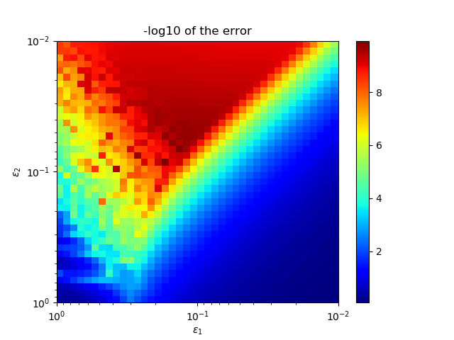
Refer to caption
Figure 7: Log of the distance from ψε1,ε20​(1ε1​ε2)\psi^{0}_{\varepsilon_{1},\varepsilon_{2}}(\frac{1}{\varepsilon_{1}\varepsilon_{2}}) to the orbit of (1,0)(1,0).
Refer to caption
Figure 8: Population transfer as a function of α\alpha for E=1E=1, ε1=0.5\varepsilon_{1}=0.5 and ε2=0.1\varepsilon_{2}=0.1.
Refer to caption
Figure 9: ε1=0.5\varepsilon_{1}=0.5, ε2=0.1\varepsilon_{2}=0.1 and α=0\alpha=0. In thick line are the trajectories corresponding to the equivalent 1st order RWA system.
Refer to caption
Figure 10: ε1​ε2=0.05\varepsilon_{1}\varepsilon_{2}=0.05, α=0\alpha=0. In thick line are the trajectories corresponding to the equivalent 1st order RWA system and in dotted line the theoretical AA trajectories.

Acknowledgements

The authors want to thank Steffen Glaser and Dominique Sugny for their very useful comments.

This work was supported by the ANR project SRGI ANR-15-CE40-0018, and by the ANR project Quaco ANR-17-CE40-0007-01.

References

  • [1] A. A. Agrachev and Y. L. Sachkov. Control theory from the geometric viewpoint, volume 87 of Encyclopaedia of Mathematical Sciences. Springer-Verlag, Berlin, 2004. Control Theory and Optimization, II.
  • [2] S. Ashhab, J. R. Johansson, A. M. Zagoskin, and F. Nori. Two-level systems driven by large-amplitude fields. Phys. Rev. A, 75:063414, Jun 2007.
  • [3] N. Augier, U. Boscain, and M. Sigalotti. Adiabatic ensemble control of a continuum of quantum systems. SIAM J. Control Optim., 56(6):4045–4068, 2018.
  • [4] N. Augier, U. Boscain, and M. Sigalotti. On the compatibility between the adiabatic and the rotating wave approximations in quantum control. In CDC 2019 - 58th Conference on Decision and Control, Nice, France, Dec. 2019.
  • [5] N. Augier, U. Boscain, and M. Sigalotti. Semi-conical eigenvalue intersections and the ensemble controllability problem for quantum systems. Math. Control Relat. Fields, 10(4):877–911, 2020.
  • [6] N. Augier, U. Boscain, and M. Sigalotti. Effective adiabatic control of a decoupled hamiltonian obtained by rotating wave approximation. Preprint HAL : https://hal.inria.fr/hal-02562363, 2021.
  • [7] K. Beauchard, J.-M. Coron, and P. Rouchon. Controllability issues for continuous-spectrum systems and ensemble controllability of Bloch equations. Comm. Math. Phys., 296(2):525–557, 2010.
  • [8] X. Cao, J. Q. You, H. Zheng, A. G. Kofman, and F. Nori. Dynamics and quantum zeno effect for a qubit in either a low- or high-frequency bath beyond the rotating-wave approximation. Phys. Rev. A, 82:022119, Aug 2010.
  • [9] M. Garwood and L. DelaBarre. The return of the frequency sweep: Designing adiabatic pulses for contemporary NMR. Journal of magnetic resonance (San Diego, Calif.: 1997), 153:155–77, 01 2002.
  • [10] H. Jo, H.-g. Lee, S. Guérin, and J. Ahn. Robust two-level system control by a detuned and chirped laser pulse. Physical Review A, 96(3), Sep 2017.
  • [11] Z. Leghtas, A. Sarlette, and P. Rouchon. Adiabatic passage and ensemble control of quantum systems. Journal of Physics B, 44(15), 2011.
  • [12] J.-S. Li and N. Khaneja. Control of inhomogeneous quantum ensembles. Phys. Rev. A, 73:030302, 2006.
  • [13] J.-S. Li and N. Khaneja. Ensemble control of Bloch equations. IEEE Trans. Automat. Control, 54(3):528–536, 2009.
  • [14] U. A. Maciel Neto, P. S. Pereira da Silva, K. Beauchard, and P. Rouchon. H1{H}^{1}-control of an ensemble of half-spin systems replacing Rabi pulses by adiabatic following. In Proceedings of the 58th IEEE Conference on Decision and Control, 2019.
  • [15] V. Malinovsky and J. Krause. General theory of population transfer by adiabatic rapid passage with intense, chirped laser pulses. Eur. Phys. J. D, 1450:147–155, 05 2001.
  • [16] M. H. Mittleman. Introduction to the theory of laser-atom interactions. Springer Science & Business Media, 2013.
  • [17] P. Rouchon. Quantum systems and control 1. Revue Africaine de la Recherche en Informatique et Mathématiques Appliquées, Volume 9, Conference in Honor of Claude Lobry, 2008.
  • [18] J. Sanders, F. Verhulst, and J. Murdock. Averaging methods in nonlinear dynamical systems. Number 59 in Applied Mathematical Sciences. Springer, 2007.
  • [19] J. Scheuer, X. Kong, R. S. Said, J. Chen, A. Kurz, L. Marseglia, J. Du, P. R. Hemmer, S. Montangero, T. Calarco, B. Naydenov, and F. Jelezko. Precise qubit control beyond the rotating wave approximation. New Journal of Physics, 16(9):093022, sep 2014.
  • [20] P. Shapiro, Moshe; Brumer. Quantum Control of Molecular Processes. John Wiley & Sons, Ltd, 2012.
  • [21] B. Shore. Coherent manipulations of atoms using laser light. Acta Physica Slovaca, 58, 07 2008.
  • [22] B. W. Shore. Manipulating Quantum Structures Using Laser Pulses. Cambridge University Press, 2011.
  • [23] C.-M. Simon, T. Belhadj, B. Chatel, T. Amand, P. Renucci, A. Lemaitre, O. Krebs, P. A. Dalgarno, R. J. Warburton, X. Marie, and B. Urbaszek. Robust quantum dot exciton generation via adiabatic passage with frequency-swept optical pulses. Phys. Rev. Lett., 106:166801, Apr 2011.
  • [24] S. Teufel. Adiabatic perturbation theory in quantum dynamics, volume 1821 of Lecture Notes in Mathematics. Springer-Verlag, Berlin, 2003.
  • [25] B. T. Torosov, S. Guérin, and N. V. Vitanov. High-fidelity adiabatic passage by composite sequences of chirped pulses. Phys. Rev. Lett., 106:233001, Jun 2011.
  • [26] N. V. Vitanov, M. Fleischhauer, B. W. Shore, and K. Bergmann. Coherent manipulation of atoms and molecules by sequential laser pulses. Advances in Atomic Molecular and Optical Physics, 46:55–190, Jan. 2001.
  • [27] Y. Wu, I. M. Piper, M. Ediger, P. Brereton, E. R. Schmidgall, P. R. Eastham, M. Hugues, M. Hopkinson, and R. T. Phillips. Population inversion in a single InGaAs quantum dot using the method of adiabatic rapid passage. Phys. Rev. Lett., 106:067401, Feb 2011.