Hybrid Particle-Field Molecular Dynamics Under Constant Pressure

Sigbjørn Løland Bore email: s.l.bore@kjemi.uio.no Affiliation: Department of Chemistry, and Hylleraas Centre for Quantum Molecular Sciences, University of Oslo, PO Box 1033 Blindern, 0315 Oslo, Norway Hima Bindu Kolli Present address: Department of Physics and Astronomy, The University of Sheffield, United Kingdom Affiliation: Department of Chemistry, and Hylleraas Centre for Quantum Molecular Sciences, University of Oslo, PO Box 1033 Blindern, 0315 Oslo, Norway Antonio De Nicola Affiliation: Department of Organic Materials Science, Yamagata University, 4-3-16 Jonan Yonezawa, Yamagata-ken 992-8510, Japan Maksym Byshkin Affiliation: Institute of Computational Science, Università della Svizzera italiana, 6900 Lugano, Switzerland Toshihiro Kawakatsu Affiliation: Department of Physics, Tohoku University, Aoba, Aramaki, Aoba-ku, Sendai 980-8578, Japan Giuseppe Milano Affiliation: Department of Organic Materials Science, Yamagata University, 4-3-16 Jonan Yonezawa, Yamagata-ken 992-8510, Japan Michele Cascella email: michele.cascella@kjemi.uio.no Affiliation: Department of Chemistry, and Hylleraas Centre for Quantum Molecular Sciences, University of Oslo, PO Box 1033 Blindern, 0315 Oslo, Norway

August 11, 2026

Abstract

Hybrid particle-field methods are computationally efficient approaches for modelling soft matter systems. So far applications of these methodologies have been limited to constant volume conditions. Here, we reformulate particle-field interactions to represent systems coupled to constant external pressure. First, we show that the commonly used particle-field energy functional can be modified to model and parameterize the isotropic contributions to the pressure tensor without interfering with the microscopic forces on the particles. Second, we employ a square gradient particle-field interaction term to model non-isotropic contributions to the pressure tensor, such as in surface tension phenomena. This formulation is implemented within the hybrid particle-field molecular dynamics approach and is tested on a series of model systems. Simulations of a homogeneous water box demonstrate that it is possible to parameterize the equation of state to reproduce any target density for a given external pressure. Moreover, the same parameterization is transferable to systems of similar coarse-grained mapping resolution. Finally, we evaluate the feasibility of the proposed approach on coarse-grained models of phospholipids, finding that the term between water and the lipid hydrocarbon tails is alone sufficient to reproduce the experimental area per lipid in constant-pressure simulations, and to produce a qualitatively correct lateral pressure profile.

I Introduction

Hybrid particle-field simulations (hPF) are a group of computationally efficient approaches for studying mesoscale soft matter systems with molecular resolution. Daoulas and Müller 2006; Müller 2011; Milano and Kawakatsu 2009; Vogiatzis, Megariotis, and Theodorou 2017 In hPF models, computationally expensive, intermolecular pair interaction potentials are replaced by an inhomogeneous external potential that is functionally dependent on the densities of the particles composing the system. As a consequence, the motion of the moieties composing the system decouples, yielding a substantial simplification for the sampling of the phase space. From an algorithmic point of view, the hPF methods are efficiently represented by particle-mesh approaches, giving excellent parallelization efficiency Zhao et al. 2012. Very recently, a GPU-based implementation of the Monte Carlo based hPF (single chain in mean field) set a new milestone with simulations of polymer melts with 10 billion particles Schneider and Müller 2019.

Coupling hPF to molecular dynamics algorithms has widened the range of applicability of hPF systems, from more conventional soft polymer mixtures to biological systems Milano, Kawakatsu, and De Nicola 2013; Soares et al. 2017; Cascella and Vanni 2015; Marrink et al. 2019. Examples from the literature include nanocomposites, nanoparticles, percolation phenomena in carbon nanotubes De Nicola et al. 2016; Zhao et al. 2016; Munaò et al. 2018; Munaò et al. ress, lamellar and nonlamellar phases of phospholipids De Nicola et al. 2012; De Nicola et al. 2011, and more recently polypeptides, and polyelectrolytes Zhu et al. 2016; Kolli et al. 2018; Bore et al. 2019; Nicola et al. 2020.

Despite the growing level of maturity reached by hPF simulations, to the best of the authors knowledge, all works that have appeared in the literature so far have been restricted to canonical, constant volume ( $NVT$ ) thermodynamic conditions. In fact, the study of many important phenomena requires targeting constant pressure conditions ( $NPT$ ). For example, structural and dynamic properties of lipid membranes are typically defined at fixed tension (prominently, at zero tension), which are best represented within the $NPT$ ensemble. Furthermore, the average density of heterogeneous or multiphase systems often cannot straightforwardly be determined from the bulk values of its constituents, making it difficult to establish physically sound $NVT$ conditions in the absence of a preliminary equilibration at $NPT$ , or of additional information from other experimental or computational sources.

The main issue related to the calculation of the pressure in hPF resides in determining the contribution by the particle-field interaction energy. In particular, contrary to ordinary pair potentials, such term cannot be computed from the virial of the intermolecular forces. In 2003, Tyler and Morse Tyler and Morse 2003 proposed a derivation of the pressure in a continuum self-consistent field theory formalism by computing the change in free energy upon a change in the volume. More recently, some of us proposed a first formulation for pressure in hPF Milano and Kawakatsu 2010 by a virtual displacement approach Brown and Neyertz 1995, obtaining a good correspondence of the equation of state for polymer chains compared to that derived from particle-based simulations. In a very recent publication Ting and Müller 2017, Ting and Müller also considered local pressure profiles in multiphase systems within self-consistent field theory, putting particular emphasis on bilayer structures. With the added novelty of using Kirkwood-Irving assignment of pressure contributions from bonded terms, they obtained excellent agreement between interface properties computed from local pressure profiles and thermodynamic considerations, demonstrating also the usefulness of local pressure profiles in density field based methods. Ting and Müller 2017 Finally, Sgouros et al. Sgouros et al. 2018 derived the pressure for hPF using the thermodynamic definition of the pressure tensor Lustig, Shay Jr, and Caruthers 1996.

Despite the capability of deriving and computing the pressure in $NVT$ conditions, two important issues hinder hPF simulations under constant pressure. First, the interaction energy functionals commonly used in hPF simulations Milano and Kawakatsu 2009; Daoulas and Müller 2006 are not designed to give a realistic representation of the equation of state. Second, as can be seen from inspection of density field contributions in refs. Ting and Müller 2017; Milano and Kawakatsu 2010 and is emphasized in ref. Sgouros et al. 2018, pure density terms contribute only isotropically to the pressure. This is particularly detrimental for interfacial phenomena, where the appearance of any surface tension is only limited to the eventual non-isotropic orientation of the bonded terms for spatially organized molecules.

In density field approaches, the square gradient term is one of the simplest ways to model the surface tension explicitly. Such terms have been used all the way back to pioneering works of van der Waals on one-component systems van der Waals 1979 and by Cahn and Hilliard on two-component systems Cahn and Hilliard 1958. Particularly relevant for the hPF method is its recent implementation in hPF-Brownian dynamics to model polymer-air interfaces Sgouros et al. 2018. Here, we reformulate the interaction energy for hPF simulations, also including anisotropic square gradient terms, to allow for an appropriate representation of the equation of state, making it possible to simulate constant pressure conditions.

II $NPT$ ensemble Hybrid Particle-Field

II.1 hPF Hamiltonian

We consider a system formed by $N$ molecules subject to the following Hamiltonian:

H=\sum\limits_{m=1}^{N}H_{0}(\{\mathbf{r},\dot{\mathbf{r}}\}_{m})+W[\{\phi(\mathbf{r}),\mbox{\boldmath$\nabla$}\phi\}].

(1)

$H_{0}$ is the single-particle Hamiltonian for the $m$ -th molecule:

H_{0}=T(\{\dot{\mathbf{r}}\}_{m})+U_{0}(\{\mathbf{r}\}_{m}),

(2)

where $T$ and $U_{0}$ are its kinetic and intramolecular potential energies. In hPF models, intermolecular interactions are typically taken into account by the interaction energy functional $W$ , which is implicitly dependent on the position of the particles through the set of number densities $\{\phi_{k}\}$ , where the index $k$ indicates a particle type. Here we introduce a new formulation of the energy functional, making it also dependent on density gradients $\{\mbox{\boldmath$\nabla$}\phi_{k}\}$ . We separate the interaction energy into two terms:

W[\{\phi_{k}(\mathbf{r}),\mbox{\boldmath$\nabla$}\phi_{k}\}]=W_{0}[\{\phi_{k}\}]+W_{1}[\{\mbox{\boldmath$\nabla$}\phi_{k}\}].

(3)

W₀: Flory-Huggins mixing entropy and compressibility

The original formulation for hPF under $NVT$ conditions employed the following interaction energy functional Milano and Kawakatsu 2009; Milano and Kawakatsu 2010:

W_{0}[\{\phi_{k}(\mathbf{r})\}]=\frac{1}{2\phi_{0}}\int\text{d}\mathbf{r}\left(\sum_{k\ell}\tilde{\chi}_{k\ell}\phi_{k}(\mathbf{r})\phi_{\ell}(\mathbf{r})+\frac{1}{\kappa}\left(\sum_{\ell}\phi_{\ell}(\mathbf{r})-\phi_{0}\right)^{2}\right),

(4)

where $\phi_{0}$ is the average total number density, $\tilde{\chi}_{k\ell}$ is the Flory-Huggins coupling parameter between species $k$ and $\ell$ , and $\kappa$ controls the fluctuations of the local density. To generalize this formulation to $NPT$ conditions, we propose the following modified interaction energy:

W_{0}[\{\phi_{k}(\mathbf{r})\}]=\frac{1}{2\rho_{0}}\int\text{d}\mathbf{r}\left(\sum_{k\ell}\tilde{\chi}_{k\ell}\phi_{k}(\mathbf{r})\phi_{\ell}(\mathbf{r})+\frac{1}{\kappa}\left(\sum_{\ell}\phi_{\ell}(\mathbf{r})-a\right)^{2}\right).

(5)

Here $\rho_{0}=1/v_{0}$ is a constant related to the scale of coarse graining, where $v_{0}$ is the molecular volume of the coarse grained particles. $a$ is an independent parameter of the equation of state with the dimension of a number density. The corresponding external potential is given by:

V_{0,k}(\mathbf{r})=\frac{\delta W_{0}[{\phi_{k}(\mathbf{r})}]}{\delta\phi_{k}(\mathbf{r})}=\frac{1}{\rho_{0}}\left(\sum_{\ell}\tilde{\chi}_{k\ell}\phi_{\ell}(\mathbf{r})+\frac{1}{\kappa}\left(\sum_{\ell}\phi_{\ell}(\mathbf{r})-a\right)\right).

(6)

We emphasize that because the parameter $a$ gives a constant contribution the potential $V_{0,k}$ , it does not affect the forces acting on the particles. We also note that in the case of $\rho_{0}=\phi_{0}=a$ , this new potential becomes strictly the same as the one used in the $NVT$ formulation.

$W_{1}$ : Square gradient interactions

To model interfaces we introduce a square gradient term to the interaction energy Sgouros et al. 2018; Onuki 2007 dependent on multiple species:

W_{1}[\mbox{\boldmath$\nabla$}\phi]=\frac{1}{2\rho_{0}}\sum_{k,\ell}\int\text{d}\mathbf{r}~K_{k\ell}\mbox{\boldmath$\nabla$}\phi_{k}(\mathbf{r})\cdot\mbox{\boldmath$\nabla$}\phi_{\ell}(\mathbf{r}),

(7)

where $K_{k\ell}$ is a coupling constant between the gradients of species $k$ and $\ell$ . The corresponding external potential is given by (see SI .1.1):

\displaystyle V_{1,k}(\mathbf{r})=-\sum_{\ell=1}\frac{K_{k\ell}}{\rho_{0}}\nabla^{2}\phi_{\ell}(\mathbf{r}).

(8)

II.2 Calculation of the pressure in hPF

We calculate the pressure using a derivation similar to the one used by Hünenberger for the reciprocal space part of Ewald summation Hünenberger 2002. The pressure inside a simulation box with side lengths $L_{\mu}$ and volume $V$ is given by:

P_{\mu}=\frac{2T_{\mu}-\text{Vir}_{\mu}(\{\mathbf{r},\mathbf{L}\})}{V}

(9)

where $T_{\mu}$ denotes a Cartesian component of kinetic energy and

\text{Vir}_{\mu}=L_{\mu}\frac{\partial U_{\text{tot}}}{\partial L_{\mu}}

(10)

is obtained directly from the potential energy of the system $U_{\text{tot}}$ , defined as:

U_{\text{tot}}=\sum_{m=1}^{N}U_{0}(\{\mathbf{r}\}_{m})+W_{0}[\{\phi\}]+W_{1}[\{\mbox{\boldmath$\nabla$}\phi\}].

(11)

The bonded interactions ( $U_{0}(\{\mathbf{r}\}_{m})$ ) contribute to the virial term as in ordinary molecular dynamics. The interaction energy contributions to the pressure are computed as:

P_{0,\mu}=-\frac{L_{\mu}}{V}\frac{\partial W_{0}[\{\phi\}]}{\partial L_{\mu}},\quad P_{1,\mu}=-\frac{L_{\mu}}{V}\frac{\partial W_{1}[\{\mbox{\boldmath$\nabla$}\phi\}]}{\partial L_{\mu}},

(12)

corresponding to (see SI .1.2 for their derivation):


$\displaystyle P_{0,\mu}$	$\displaystyle=\frac{1}{V}\int\text{d}\mathbf{r}~\frac{1}{\rho_{0}}\left(\frac{1}{2}\sum_{k\ell}\tilde{\chi}_{k\ell}\phi_{k}(\mathbf{r})\phi_{\ell}(\mathbf{r})+\frac{1}{2\kappa}\left(\left(\sum_{\ell}\phi_{\ell}(\mathbf{r})\right)^{2}-a^{2}\right)\right),$	(13a)
$\displaystyle P_{1,\mu}$	$\displaystyle=\frac{1}{V}\int\text{d}\mathbf{r}~\sum_{k\ell}\frac{K_{k\ell}}{\rho_{0}}\left(\frac{1}{2}\mbox{\boldmath$\nabla$}\phi_{k}(\mathbf{r})\cdot\mbox{\boldmath$\nabla$}\phi_{\ell}(\mathbf{r})+\nabla_{\mu}\phi_{k}(\mathbf{r})\nabla_{\mu}\phi_{\ell}(\mathbf{r})\right).$	(13b)

The total pressure in a direction $\mu$ is thus given by:

P_{\mu}=\frac{2T_{\mu}}{V}+\frac{1}{V}\sum_{i}\left[-\frac{\partial U_{0}(\mathbf{r}_{i})}{\partial r_{i,\mu}}\cdot r_{i,\mu}\right]+P_{0,\mu}+P_{1,\mu}

(14)

Here we note the following: (i) Although $a$ gives no contributions to the force, it gives rise to a nonzero pressure. This gives added flexibility to control the isotropic pressure, similarly to the constant term in the stiffened gas equation of state Le Métayer and Saurel 2016. (ii) The contribution of $W_{0}$ to the pressure is isotropic, while the contribution of $W_{1}$ is not. (iii) The local pressure density (the integrand in (13b)) does not contain a Laplace term as reported in refs. Onuki 2007; Sgouros et al. 2018. However, as shown in SI .1.2, the expressions are equivalent.

III Computational details

III.1 hPF-MD simulations

The model described in the previous section was implemented into hPF-molecular dynamics software OCCAM Zhao et al. 2012. This enables the possibility of sample configurations of the molecular system governed by our new hPF Hamiltonian (1) following directly the evolution of the corresponding equations of motion. The forces on the $i$ -th particle of type $k$ due to $W_{0}$ and $W_{1}$ are computed from the gradients of the external potentials $V_{0,k}(\mathbf{r})$ and $V_{1,k}(\mathbf{r})$ :

\mathbf{F}_{0,i}=-\mbox{\boldmath$\nabla$}V_{0,k}(\mathbf{r}_{i}),\quad\mathbf{F}_{1,i}=-\mbox{\boldmath$\nabla$}V_{1,k}(\mathbf{r}_{i}).

(15)

by a particle mesh approach De Nicola et al. 2011. First, particles are distributed onto a different Cartesian grid for each species $k$ by linear interpolation to the nearest vertices (cloud-in-cell). Derivatives are computed on a staggered grid by finite differences. Finally, the derivatives are interpolated back onto the particles giving the forces. As shown in ref. De Nicola et al. 2011, the external potentials are slow variables, and can be updated with good approximation at intervals of up to $\sim$ 100 steps De Nicola et al. 2011, yielding efficient parallelization Zhao et al. 2012.

III.2 Computation of square gradient forces

The computation of the external potential due to the square gradient term $W_{1}$ involves computing the Laplacian of the densities. To obtain a rotational invariant estimate without the appearance of spurious oscillations, we employ a spectral approach Canuto et al. 2006 filtering out fast oscillations of the derivatives in Fourier space. The filtering is done by convolution:

\tilde{\phi}_{k}(\mathbf{r})=\int\text{d}\mathbf{u}~\phi_{k}(\mathbf{r}-\mathbf{u})H(\mathbf{u}).

(16)

The tilde symbol denotes filtered densities by the applied filter $H$ . The corresponding external potential is given by:

\displaystyle V_{1,k}(\mathbf{r})=-\sum^{M}_{\ell=1}\frac{K_{k\ell}}{\rho_{0}}\int\text{d}\mathbf{y}~H(\mathbf{r}-\mathbf{y})\nabla^{2}\tilde{\phi}_{\ell}(\mathbf{y}).

(17)

which takes the following simple expression in Fourier space (see SI .1.1 for its derivation):

\hat{V}_{1,k}(\mathbf{q})=\sum^{M}_{\ell=1}\frac{K_{k\ell}}{\rho_{0}}q^{2}H^{2}(\mathbf{q})\hat{\phi}_{\ell}(\mathbf{q}).

(18)

Real space values are computed by backwards Fast Fourier Transform routines (FFT). For consistency, the gradients in $P_{1}$ are also filtered with the same filter $H$ . Details on the filtering algorithm are provided in SI .2.1.

III.3 Barostat

We employ the Berendsen barostat Berendsen et al. 1984 with isotropic coupling for isotropic systems, and semiisotropic coupling for lipid bilayers. The efficiency of the hPF-MD approach is dependent on having i) little communication among processors and ii) avoiding heavy calculation (typically involving the grid) between density updates. Similarly to the multi-time-step approach used in the GPU version of Tinker-OpenMM Harger and Ren 2019, we average contributions from bonded terms and keep volume and field contributions constant between density update steps.

III.4 Simulation details

We tested our model on a set of homogeneous and inhomogeneous systems. Details on the composition of each individual system, as well as information about other simulation parameters are given in SI .3. The data that support the findings of this study are available from the corresponding author upon reasonable request.

IV Results and discussion

IV.1 Homogeneous system: Water

Refer to caption — Figure 1: Parameterization of water for $NPT$ simulation. (A) Simulation box of water. (B) Pressure as function of $\kappa$ for $a=0$ . (C) Calibration of $a$ to obtain an internal pressure of $1\text{\,}\mathrm{b}\mathrm{a}\mathrm{r}$ as function of $\kappa$ . The least square fit line is $a(\kappa)=8.54+18.61\kappa$ . (D) Equilibration of a overly dense liquid by $NPT$ simulation.

Within the hPF model, the representation of a homogeneous phase requires the consideration of the interaction energy $W_{0}$ only. Furthermore, considering a single-component system, the forces are only dependent on its compressibility term. In Fig. 1 we report the parameterization of pure liquid water employing the commonly used explicit bead model in hPF-MD where four water molecules are mapped into a single body De Nicola et al. 2011 (Fig. 1A). Such a mapping implies a molecular volume per bead $v_{0}=$0.120\text{\,}\mathrm{n}\mathrm{m}^{3}$$ , thereby $\rho_{0}=1/v_{0}=$8.33\text{\,}\mathrm{n}\mathrm{m}^{-3}$$ . In Fig. 1B, the pressure under $NVT$ conditions is plotted as function of $\kappa$ for a system with a density of $995\text{\,}\mathrm{k}\mathrm{g}\,\mathrm{m}^{-3}$ and temperature of $300\text{\,}\mathrm{K}$ , using $a=$0\text{\,}\mathrm{n}\mathrm{m}^{-3}$$ . The combination of the two positive definite kinetic energy and compressibility terms produce an average internal pressure $\left\langle P\right\rangle\gg$ $1\text{\,}\mathrm{b}\mathrm{a}\mathrm{r}$ . From (14) and (13), it is possible to predict the value of $a$ :

a=\sqrt{(\left<P\right>_{a=0}-P_{0})/(2\kappa\rho_{0})},

(19)

that would yield an equilibrium value $\langle P\rangle_{a}=P_{0}$ , where $P_{0}$ is any target pressure of choice. Inserting $P_{0}=$1\text{\,}\mathrm{b}\mathrm{a}\mathrm{r}$$ and values of $\left<P\right>_{a=0}$ into (19), we find a parameterization of $a$ as function of $\kappa$ (Fig. 1C) which yields a pressure of $1\text{\,}\mathrm{b}\mathrm{a}\mathrm{r}$ for a density of $995\text{\,}\mathrm{k}\mathrm{g}\,\mathrm{m}^{-3}$ at $300\text{\,}\mathrm{K}$ . The parameterization of $a(\kappa)$ is fitted well by a linear regression line. Using this regression line we find, for three commonly used values of $\kappa={0.03},~0.05,~$0.10\text{\,}\mathrm{k}\mathrm{J}^{-1}\mathrm{m}\mathrm{o}\mathrm{l}$$ , $a=9.10,~9.47,~$10.40\text{\,}\mathrm{n}\mathrm{m}^{-3}$$ respectively. Having parameterized $a$ , we can now simulate the water model under $NPT$ conditions. Fig. 1D reports the time evolution of total mass density $\rho$ under $NPT$ conditions with barostat pressure of $1\text{\,}\mathrm{b}\mathrm{a}\mathrm{r}$ and temperature of $300\text{\,}\mathrm{K}$ for a water system with an initial density of $1100\text{\,}\mathrm{k}\mathrm{g}\,\mathrm{m}^{-3}$ . For the three values of $\kappa$ the density equilibrates to the correct density. In the next systems, if not otherwise stated, we adopt $\kappa=$0.05\text{\,}\mathrm{k}\mathrm{J}^{-1}\mathrm{m}\mathrm{o}\mathrm{l}$$ and $a=$9.47\text{\,}\mathrm{n}\mathrm{m}^{-3}$$ .

IV.2 Binary mixture

Phase separation

We consider a toy binary mixture between two ideal fluids. The two components differ only by $\tilde{\chi}_{\text{AB}}$ in the potential energy term $W_{0}$ . In Fig. 2 we survey the state of this mixture by plotting its total density as a function of $\tilde{\chi}_{\text{AB}}$ at $1\text{\,}\mathrm{b}\mathrm{a}\mathrm{r}$ . The total density of the mixture exhibits a strong excess volume effect, where the density of the mixture is different from its components. For negative values of $\tilde{\chi}_{\text{AB}}$ , mixing of the two fluids is favourable, and the density increases. For positive values of $\tilde{\chi}_{\text{AB}}$ the density is lower and stabilizes to a constant value for high values of $\tilde{\chi}_{\text{AB}}$ . The stabilization can be interpreted from the snapshot at $\tilde{\chi}_{\text{AB}}=$30\text{\,}\mathrm{k}\mathrm{J}\,\mathrm{m}\mathrm{o}\mathrm{l}^{-1}$$ as the formation of a sharp interface between the two phases. The abrupt change in the first derivative of the total density at about $\tilde{\chi}_{\text{AB}}=$5\text{\,}\mathrm{k}\mathrm{J}\,\mathrm{m}\mathrm{o}\mathrm{l}^{-1}$$ signals a phase transition. This is further evidenced by the snapshots showing a transition from miscible to phase-separated fluids before and after $\tilde{\chi}_{\text{AB}}=$5\text{\,}\mathrm{k}\mathrm{J}\,\mathrm{m}\mathrm{o}\mathrm{l}^{-1}$$ .

Ideal water/oil droplet

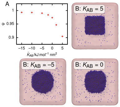
While the $\tilde{\chi}_{\text{AB}}$ term in $W_{0}$ controls the partitioning and the level of phase separation between the two liquids, the interaction energy $W_{1}$ is necessary for modelling interfacial properties, and in particular surface tension. In the case of a binary system, $W_{1}$ requires the definition of only one parameter $K_{\text{AB}}$ to control the surface interaction between the two phases. We survey how $K_{\text{AB}}$ affects interfaces by simulating an ideal oil droplet (particle type A) in water (particle type B, constituting 90% of the particles in the simulation) and by computing its sphericity for different values of $K_{\text{AB}}$ (Fig. 3A). The sphericity $\Psi$ is defined by the equation Wadell 1935:

\Psi\equiv\frac{\pi^{1/3}6V^{2/3}}{A},

(20)

where $A$ and $V$ are the surface area and the volume of the droplet. For very negative values of $K_{\text{AB}}$ , we find a sphericity close to 1, corresponding to almost a perfect sphere (snapshot in Fig. 3B). This is consistent with a sphere having the lowest possible surface for a given volume. By increasing $K_{\text{AB}}$ , we lower the interfacial energy. This allows for larger surface areas of the droplet, and thus the appearance of other shapes than a sphere. In our simulations, for $K_{AB}=$0\text{\,}\mathrm{k}\mathrm{J}\,\mathrm{m}\mathrm{o}\mathrm{l}^{-1}\,\mathrm{n}\mathrm{m}^{2}$$ , we found a configuration in between sphere and cube and for $K_{\text{AB}}=$5\text{\,}\mathrm{k}\mathrm{J}\,\mathrm{m}\mathrm{o}\mathrm{l}^{-1}\,\mathrm{n}\mathrm{m}^{2}$$ we observed a configuration very close to a cube (snapshots in Fig. 3B). We note that the formation of a cube is likely affected by the orientation of the grid used to to calculate particle-field forces, which has been reported to produce cube shaped vesiclesSevink et al. 2017.

IV.3 Effect of square gradient term on lipid bilayers

To test the feasibility of the proposed approach to models with specific molecular features, we investigate a realistic model of a dipalmitoylphosphatidylcholine (DPPC) lipid bilayer in water, employing a molecular CG representation, and the corresponding $\tilde{\chi}$ interaction energy matrix present in the literature De Nicola et al. 2011, as summarized in Fig. 4. Here, we add to the preexisting model the square gradient interaction limited to only one $K_{m\ell}$ term between the hydrophobic lipid tail (C) and the water (W) beads ( $K_{\text{CW}}$ ), disregarding all other terms.

flat lipid bilayers – Surface area

$NVT$ simulations of lipid bilayers in periodic boundary conditions impose an arbitrary effective area per lipid $A$ , defined as:

A=\frac{2L_{x}L_{y}}{N},

(21)

where $L_{x},L_{y}$ are the edges of the simulation box in the $x,y$ directions spanning lipid bilayer, and $N$ is the number of assembled lipids. In this case, $NVT$ simulations allow for a controlled study of the effects of $K_{\text{CW}}$ on the morphology of the system. Fig. 5A reports equilibrated conformations for different values of $K_{\text{CW}}$ . As we start from preoptimized $\tilde{\chi}$ values to reproduce flat bilayers at $K_{\text{CW}}=$0\text{\,}\mathrm{k}\mathrm{J}\,\mathrm{m}\mathrm{o}\mathrm{l}^{-1}\,\mathrm{n}\mathrm{m}^{2}$$ , a negative value of $K_{\text{CW}}=$-6\text{\,}\mathrm{k}\mathrm{J}\,\mathrm{m}\mathrm{o}\mathrm{l}^{-1}\,\mathrm{n}\mathrm{m}^{2}$$ does not produce strong structural modifications. On the contrary, $K_{\text{CW}}=$2\text{\,}\mathrm{k}\mathrm{J}\,\mathrm{m}\mathrm{o}\mathrm{l}^{-1}\,\mathrm{n}\mathrm{m}^{2}$$ induces an abrupt change in the bilayer with the formation of visible bump within the first $190\text{\,}\mathrm{n}\mathrm{s}$ of simulations. This deformation is consistent with the fact that positive values of $K_{\text{CW}}$ promote the expansion of the interface area.

This trend can be quantified by computing the surface tension $\gamma$ of the membrane, Fig. 5B, which can be calculated from:

\gamma=\frac{1}{2}\int\text{d}z~\left(P_{\text{N}}(z)-P_{\text{L}}(z)\right).

(22)

Here, $P_{\text{N}}(z)$ and $P_{\text{L}}(z)$ are the values of the pressure in the normal and lateral directions of the membrane plane, respectively. The $1/2$ factor takes into account the presence of two interfaces. A negative value of $\gamma$ in the absence of the square gradient interaction energy indicates that the area per lipid is not at equilibrium, and the system would tend to expand laterally if let free to relax. $K_{\text{CW}}\sim$-6\text{\,}\mathrm{k}\mathrm{J}\,\mathrm{m}\mathrm{o}\mathrm{l}^{-1}\,\mathrm{n}\mathrm{m}^{2}$$ balances the two pressures, and should predict an equilibrium area per lipid at $NPT$ conditions equal to the initial target value.

Table 1: Predicted area per lipid compared against literature data from experiment and simulations.

Source	DMPC		DPPC		DSPC		DOPC
	$A/$\mathrm{n}\mathrm{m}^{2}$$	$T/$\mathrm{K}$$	$A/$\mathrm{n}\mathrm{m}^{2}$$	$T/$\mathrm{K}$$	$A/$\mathrm{n}\mathrm{m}^{2}$$	$T/$\mathrm{K}$$	$A/$\mathrm{n}\mathrm{m}^{2}$$	$T/$\mathrm{K}$$
Nagle Nagle and Tristram-Nagle 2000	0.596	323	0.630	323	-	-	0.725	303
Waheed Waheed and Edholm 2009 sim	0.625	303	0.644	323	-	-	-	-
Waheed Waheed and Edholm 2009 exp	0.606	303	0.630	323	-	-	-	-
Levine Levine et al. 2014	-	-	0.629	323	-	-	0.689	298
Petrache Petrache, Dodd, and Brown 2000	0.600	303	0.633	323	0.66	338	-	-
	0.654	323	0.671	338	-	-	-	-
hPF-MD	0.61	323	0.64	325	0.66	338	0.70	303

We thus simulated a $20\text{\,}\mathrm{n}\mathrm{m}$\times$100\text{\,}\mathrm{n}\mathrm{m}$\times$100\text{\,}\mathrm{n}\mathrm{m}$ large DPPC/water system at $NPT$ condition employing the same $a=$9.59\text{\,}\mathrm{n}\mathrm{m}^{-3}$$ determined for pure water at $325\text{\,}\mathrm{K}$ (see SI .4) and using $K_{\text{CW}}=$-6\text{\,}\mathrm{k}\mathrm{J}\,\mathrm{m}\mathrm{o}\mathrm{l}^{-1}\,\mathrm{n}\mathrm{m}^{2}$$ . After an initial relaxation, the DPPC bilayer reaches an equilibrium configuration characterized by a well defined area per lipid of $0.64\text{\,}\mathrm{n}\mathrm{m}^{2}$ (Table 1). This value is in excellent agreement with what has been previously reported in the literatureNagle and Tristram-Nagle 2000; Waheed and Edholm 2009; Petrache, Dodd, and Brown 2000.

The transferability of K ${}_{\text{CW}}$ was tested on three other lipids, namely: dimyristoylphosphatidylcholine (DMPC), distearoylphosphatidylcholine (DSPC) and dioleoylphosphatidylcholine (DOPC), which differ from DPPC only for the length of the carbon tail while retaining the same chemical structure of the polar head. As for DPPC, we used the W₀ parameters from ref. De Nicola et al. 2011; hPF-MD $NPT$ simulations ran using the same $a=9.59$ nm^-3, $K_{\text{CW}}=-6$ kJ mol^-1. Remarkably, these parameter produce in all cases excellent agreement with literature data, as presented in Table 1, indicating indeed a high level of transferability among chemically similar moieties.

Flat lipid bilayers – membrane structure

Figure 6: Density and pressure profiles for DPPC. (A) Comparison between the experimental electron density profilea (black line), hPF-MD using

K_{\text{CW}}

=0 kJ mol^-1nm² (red line),

K_{\text{CW}}=$-6\text{\,}\mathrm{k}\mathrm{J}\,\mathrm{m}\mathrm{o}\mathrm{l}^{-1}\,\mathrm{n}\mathrm{m}^{2}$

(blue line) and reference CG MARTINI model De Nicola et al. 2011. (B) Density profiles for the different bead types. Continuous lines are for hPF-MD data using

K_{\text{CW}}=$-6\text{\,}\mathrm{k}\mathrm{J}\,\mathrm{m}\mathrm{o}\mathrm{l}^{-1}\,\mathrm{n}\mathrm{m}^{2}$

, dashed lines are by De Nicola et al. De Nicola et al. 2011 at

NVT

conditions without a square gradient term. (C) Difference between normal and lateral components of the pressure for tensionless hPF-MD simulations compared against all-atom pressure profiles by Lindahl and Edholm Lindahl and Edholm 2000. Two different scales are used for the

y

-axis for the two models. (D) Contributions to the pressure difference shown in (C) from density field, bonded, and angular interactions.

We survey the effect of $K_{\text{CW}}$ on the equilibrium structure of the bilayer by computing the electron density profiles along the membrane normal axis for a small DPPC lipid bilayer (See SI .3.2 for a detailed system description). Fig. 6A reports a comparison between the density profiles from experiment, a CG simulation using the MARTINI force fieldMarrink et al. 2007, reference hPF simulations under $NVT$ without the square gradient term, and hPF in $NPT$ with $K_{\text{CW}}=$-6\text{\,}\mathrm{k}\mathrm{J}\,\mathrm{m}\mathrm{o}\mathrm{l}^{-1}\,\mathrm{n}\mathrm{m}^{2}$$ . All the profiles exhibit the peaks at the head and low electron density in the middle of the bilayer. The profile obtained with $K_{\text{CW}}=$-6\text{\,}\mathrm{k}\mathrm{J}\,\mathrm{m}\mathrm{o}\mathrm{l}^{-1}\,\mathrm{n}\mathrm{m}^{2}$$ has better agreement with experiment and MARTINI in the middle of the bilayer, showing instead some excessive elongation in the position of the polar head beads. This trend is corroborated by drawing the individual bead contributions to the density profile, as shown in Fig. 6B. Such opposite trends are not entirely surprising, keeping in mind that the square gradient term has been applied to the carbon tails only, while the polar head have not been corrected by any surface tension contribution. The current results suggest that by an appropriate calibration of the whole $K_{\ell m}$ matrix, the square gradient term can improve significantly the agreement between hPF and its underlying CG model. Interestingly, the peaks of the individual beads appear sharper, indicating a more regular bilayer compared to hPF $NVT$ simulations.

We also computed local pressure profile, using the values of $P_{0}$ and $P_{1}$ at the vertices of the mesh, and Kirkwood-Irving assignment of bonded virials.Sonne, Hansen, and Peters 2005 Fig. 6C,D report the local difference between normal and lateral pressure computed with hPF-MD and all-atom by Lindahl,Lindahl and Edholm 2000 and the contributions by the different terms of the Hamiltonian. While the magnitude of the all-atom pressure is about four times that of hPF-MD, we nevertheless identify the appearance of three key qualitative features: the presence of a negative peak between water and the lipid heads, a positive peak in between heads and tails, and a rather flat region in the tail part. Unlike all-atom simulations, the hPF profile has an positive sign to the pressure difference at the carbon tails, indicating compressed carbon tails in the normal direction. We note that this may be part an artifact of the coarseness of the mesh, which can cause a spill out of pressure into the middle part of the membrane, as well as by the absence of a square gradient terms between water and glycerol or polar head beads. The local pressure contributions from $P_{0}$ and $P_{1}$ were computed at the vertices of the mesh. This is at one hand rigorous as it avoids subtleties related to local pressure assignment, however higher resolution would be advantageous for computing properties from the local pressure profiles. A natural route for achieving higher resolution assignment of pressure would be to follow the procedure proposed in ref. Sega, Fábián, and Jedlovszky 2016; Sonne, Hansen, and Peters 2005 by Harasima assignment.Harasima 1958

Our simulations present a very flat bilayer without the detection of significant undulations on the tensionless surface of the bilayer. The stiffness of the bilayer can be quantified by computing the area compressibility as in ref. Marrink and Mark 2001.

For the DPPC lipid bilayer, in our case, we obtain $K_{A}=$22\,000\text{\,}\mathrm{m}\mathrm{N}\,\mathrm{m}^{-1}$$ . This is about two orders of magnitude larger than what has been reported in the literature Levine et al. 2014 ( $\sim$200\text{\,}\mathrm{m}\mathrm{N}\,\mathrm{m}^{-1}$$ ) confirming that the present setup produces an excessively rigid system. Although it is well known that the Berendsen barostat is not suited for studying fluctuations of the membrane Wong-ekkabut and Karttunen 2016, we stress here, in these preliminary test implementation, that we have only considered carbon water interactions for the square gradient term. Moreover, this term was naively added to $\tilde{\chi}$ parameters that were preoptimized to reproduce accurate density profiles in the absence of an explicit surface tension term, with consequent possible double counting of the repulsion between the water and the hydrophobic tails. Overall, the discrepancy on the fluctuation of the DPPC bilayer together with the qualitative but not quantitative agreement on the lateral pressure profiles indicate that $NPT$ simulation of realistic systems require a global parameterization of both the $\tilde{\chi}$ and $K_{m\ell}$ matrices, while a simple addition of the second term to the first may not be sufficient to obtain quantitatively accurate data.

V Conclusion and outlook

We presented a reformulation of the hPF interaction energy suitable for constant pressure simulations using both isotropic and anisotropic coupling. First, we modified the commonly used interaction energy by introducing an equation of state parameter $a$ . By design, this adjustment conserves the dynamics of the old formulation. Second, we introduced a square gradient term to the interaction energy to model interfacial phenomena. Particle-field contributions to the pressure were derived by considering change in free energy upon change in simulation box lengths. The equation of state parameter $a$ enters as an added constant to the pressure. The square gradient contributes to nonisotropic pressure, thereby allowing for direct modeling of surface tension. Our approach was implemented into the OCCAM code, where the dynamics of system governed by the hPF Hamiltonian was sampled by MD and pressure was coupled to the Berendsen barostat.

Testing on simple single particle fluids demonstrated how by tuning $a$ we can reproduce the densities at ambient conditions, also showing how the $\tilde{\chi}$ -term can be used to modulate variations in the partial molar volume in liquid mixtures. We also verified that the square gradient term can be tuned to control the shape of liquid droplets.

Finally, we tested the effect of the new hPF Hamiltonian on a realistic model of a phospholipid bilayer previously proposed in the literature. Interestingly, the square gradient term is not only important, but mandatory for achieving an area per lipid within the experimental range under $NPT$ conditions, as well as a qualitatively reasonable lateral pressure profile. Interestingly, we also found that the same parameterization of $a$ and $K_{\text{CW}}$ is transferable to other lipids of similar chemical composition.

Remarkably, the application of only one square gradient contribution between the carbon tails and water was sufficient to obtain a qualitatively correct physical behaviour of the lipids as well as some impressive improvement of some of their key structural features like average area per lipid, or lateral pressure profiles. Nonetheless, we found that such correction produced inconsistent variations in the lateral density profiles, and a too stiff bilayer, indicating that a consistent recalibration of the $\tilde{\chi}$ parameters as well as the use of the full $K_{m\ell}$ matrix is necessary for quantitative agreement between hPF and other higher resolution models as well as the experiment.

Accessing constant pressure conditions significantly expands the applicability of hPF simulations. For example, it is now possible predict density changes in bulk systems, or to represent surface phenomena. The future challenge is in the calibration of appropriate square gradient force constant matrices, possibily through combined global parameterizations with the bulk enery terms, aiming for quantitatively accurate description of interfaces.

VI Acknowledgments

The authors would like to acknowledge Morten Ledum for help with generating initial bilayer structures.

VII Funding

Authors acknowledge the support of the Norwegian Research Council through the CoE Hylleraas Centre for Quantum Molecular Sciences (Grant No. 262695) and the Norwegian Supercomputing Program (NOTUR) (Grant No. NN4654K). MC acknowledges funding by the Deutsche Forschungsgemeinschaft (DFG) within the project B5 of the TRR 146 (project number 233630050). HBK received funding from the European Union Horizon 2020 research and innovation program under the Marie Skłodowska-Curie Grant Agreement HYPERBIO - No 704491.

Supporting information

In this supporting information we provide the details on derivations, computational procedures, simulation setups and parameterizations, that are needed for reproducing the results obtained in this manuscript.

.1 Derivations

All derivations involving square gradient term are performed with filtered densities $\tilde{\phi}$ .

.1.1 External potential $V_{1,k}$

We compute the external potential by using the functional derivative chain rule twice:

V_{1,k}(\mathbf{r})=\frac{\delta W_{1}[\mbox{\boldmath$\nabla$}\tilde{\phi}]}{\delta\phi_{k}(\mathbf{r})}=\int\text{d}\mathbf{x}\text{d}\mathbf{y}~\frac{\delta W_{1}}{\delta\mbox{\boldmath$\nabla$}\tilde{\phi}_{k}(\mathbf{x})}\frac{\delta\mbox{\boldmath$\nabla$}\tilde{\phi}_{k}(\mathbf{x})}{\delta\tilde{\phi}_{k}(\mathbf{y})}\frac{\delta\tilde{\phi}_{k}(\mathbf{y})}{\delta\phi_{k}(\mathbf{r})}.

(23)

The terms in the integrand of (23) are given by:

\frac{\delta W_{1}}{\delta\mbox{\boldmath$\nabla$}\tilde{\phi}_{k}(\mathbf{x})}=\sum^{M}_{\ell=1}\frac{K_{k\ell}}{\rho_{0}}\mbox{\boldmath$\nabla$}\tilde{\phi}_{\ell}(\mathbf{x}),\quad\frac{\delta\mbox{\boldmath$\nabla$}\tilde{\phi}_{k}(\mathbf{x})}{\delta\tilde{\phi}_{k}(\mathbf{y})}=\mbox{\boldmath$\nabla$}_{\mathbf{x}}\delta(\mathbf{x}-\mathbf{y}),\quad\frac{\delta\tilde{\phi}_{k}(\mathbf{y})}{\delta\phi_{k}(\mathbf{r})}=H(\mathbf{r}-\mathbf{y}).

(24)

Inserting (24) into (23) yields:

	$\displaystyle V_{1,k}(\mathbf{r})$	$\displaystyle=\int\text{d}\mathbf{x}\text{d}\mathbf{y}~\sum^{M}_{\ell=1}\frac{K_{k\ell}}{\rho_{0}}\mbox{\boldmath$\nabla$}\tilde{\phi}_{\ell}(\mathbf{x})\mbox{\boldmath$\nabla$}_{\mathbf{x}}\delta(\mathbf{x}-\mathbf{y})H(\mathbf{r}-\mathbf{y})$
		$\displaystyle=\int\text{d}\mathbf{y}~H(\mathbf{r}-\mathbf{y})\int\text{d}\mathbf{x}~\sum^{M}_{\ell=1}\frac{K_{k\ell}}{\rho_{0}}\mbox{\boldmath$\nabla$}\tilde{\phi}_{\ell}(\mathbf{x})\mbox{\boldmath$\nabla$}_{\mathbf{x}}\delta(\mathbf{x}-\mathbf{y})$
		$\displaystyle=-\int\text{d}\mathbf{y}~H(\mathbf{r}-\mathbf{y})\int\text{d}\mathbf{x}~\sum^{M}_{\ell=1}\frac{K_{k\ell}}{\rho_{0}}\nabla^{2}\tilde{\phi}_{\ell}(\mathbf{x})\delta(\mathbf{x}-\mathbf{y})$
		$\displaystyle=-\sum^{M}_{\ell=1}\frac{K_{k\ell}}{\rho_{0}}\int\text{d}\mathbf{y}~H(\mathbf{r}-\mathbf{y})\nabla^{2}\tilde{\phi}_{\ell}(\mathbf{y}).$

Without filter ( $H(\mathbf{r}-\mathbf{y})=\delta(\mathbf{r}-\mathbf{y})$ ) we obtain:

V_{1,k}(\mathbf{r})=-\sum^{M}_{\ell=1}\frac{K_{k\ell}}{\rho_{0}}\nabla^{2}\tilde{\phi}_{\ell}(\mathbf{r})

(25)

.1.2 Virial terms from interaction energies

The pressure is given by the Viral Hünenberger 2002:

P_{\mu}=\frac{2K_{\mu}-\text{Vir}_{\mu}(\{\mathbf{r},\mathbf{L}\})}{V}

(26)

where

\text{Vir}_{\mu}=L_{\mu}\frac{\partial U}{\partial L_{\mu}}.

(27)

Focusing on nonbonded terms and starting with $W_{0}$ , we denote the integrand by interaction energy density $w(\{\phi(\mathbf{r})\})$ , we compute derivative with respect to box size:

	$\displaystyle\frac{\partial W_{0}}{\partial L_{\mu}}$	$\displaystyle=\int\left(\frac{\partial\text{d}\mathbf{r}}{\partial L_{\mu}}~w_{0}(\phi(\mathbf{r}))+\text{d}\mathbf{r}~\frac{\partial w_{0}(\phi(\mathbf{r}))}{\partial L_{\mu}}\right)$		(28)
		$\displaystyle=\int\left(\frac{\text{d}\mathbf{r}}{L_{\mu}}~w_{0}(\phi(\mathbf{r}))-\text{d}\mathbf{r}~\frac{\partial w_{0}(\phi(\mathbf{r}))}{\partial\phi}\frac{\phi(\mathbf{r})}{L_{\mu}}\right)$		(29)

giving:

\text{Vir}_{0,\mu}=\int\text{d}\mathbf{r}\left(w_{0}(\{\phi(\mathbf{r})\})-\sum_{\ell=1}^{M}\frac{\partial w_{0}(\{\phi(\mathbf{r})\})}{\partial\phi_{\ell}(\mathbf{r})}\phi_{\ell}(\mathbf{r})\right).

(30)

Inserting the energy density:

\text{Vir}_{0,\mu}=-\int\text{d}\mathbf{r}~\frac{1}{\rho_{0}}\left(\frac{1}{2}\sum_{k\ell}\tilde{\chi}_{k\ell}\phi_{k}(\mathbf{r})\phi_{\ell}(\mathbf{r})+\frac{1}{2\kappa}\left(\phi(\mathbf{r})^{2}-a^{2}\right)\right)

(31)

We compute interface virial of $W_{1}$ by:

	$\displaystyle\frac{\partial W_{1}}{\partial L_{\mu}}$	$\displaystyle=\int\left(\frac{\partial\text{d}\mathbf{r}}{\partial L_{\mu}}~w([\mbox{\boldmath$\nabla$}\tilde{\phi}(\mathbf{r})])+\text{d}\mathbf{r}~\frac{\partial w([\mbox{\boldmath$\nabla$}\tilde{\phi}(\mathbf{r})])}{\partial L_{\mu}}\right)$		(32)
		$\displaystyle=\int\left(\frac{\text{d}\mathbf{r}}{L_{\mu}}~w([\mbox{\boldmath$\nabla$}\tilde{\phi}(\mathbf{r})])+\text{d}\mathbf{r}~\frac{\partial w([\mbox{\boldmath$\nabla$}\tilde{\phi}(\mathbf{r})])}{\partial\nabla_{\nu}\tilde{\phi}(\mathbf{r})}\frac{\partial\nabla_{\nu}\tilde{\phi}(\mathbf{r})}{\partial L_{\mu}}\right).$		(33)

The last partial derivative is given by:

	$\displaystyle\frac{\partial}{\partial L_{\mu}}\left(\nabla_{\nu}\tilde{\phi}(\mathbf{r})\right)$	$\displaystyle=\left(\frac{\partial}{\partial L_{\mu}}\nabla_{\nu}\right)\tilde{\phi}(\mathbf{r})+\nabla_{\nu}\frac{\partial\tilde{\phi}(\mathbf{r})}{\partial L_{\mu}}$		(34)
		$\displaystyle=-\frac{\delta_{\mu\nu}}{L_{\mu}}\nabla_{\nu}\tilde{\phi}(\mathbf{r})+\nabla_{\nu}\frac{\partial\tilde{\phi}(\mathbf{r})}{\partial L_{\mu}}.$		(35)

The partial derivative filtered density with respect to box lengths depends on the filter. This dependence is easily understood by using the Fourier transform:

$\displaystyle\frac{\partial\tilde{\phi}(\mathbf{r})}{\partial L_{\mu}}=$	$\displaystyle\frac{\partial}{\partial L_{\mu}}\int\text{d}\mathbf{q}~\tilde{\phi}(\mathbf{q})e^{-i\mathbf{q}\mathbf{r}}=\frac{\partial}{\partial L_{\mu}}\int\text{d}\mathbf{q}~\hat{\phi}(\mathbf{q})\hat{H}(\mathbf{k})e^{-i\mathbf{q}\mathbf{r}}$	(36)
$\displaystyle=$	$\displaystyle\int\left(\frac{\partial\text{d}\mathbf{q}}{\partial L_{\mu}}\hat{\phi}(\mathbf{q})\hat{H}(\mathbf{k})e^{-i\mathbf{q}\mathbf{r}}+\text{d}\mathbf{q}\frac{\partial\hat{\phi}(\mathbf{q})}{\partial L_{\mu}}\hat{H}(\mathbf{k})e^{-i\mathbf{q}\mathbf{r}}\right.+$	(37)
	$\displaystyle\left.\text{d}\mathbf{q}\hat{\phi}(\mathbf{q})\hat{H}(\mathbf{k})\frac{\partial e^{-i\mathbf{q}\mathbf{r}}}{\partial L_{\mu}}+\text{d}\mathbf{q}\hat{\phi}(\mathbf{q})\frac{\partial\hat{H}(\mathbf{k})}{\partial L_{\mu}}e^{-i\mathbf{q}\mathbf{r}}\right).$	(38)

The contributions from the three first terms are given by:

\frac{\partial\text{d}\mathbf{q}}{\partial L_{\mu}}=-\frac{\text{d}\mathbf{q}}{L_{\mu}},\quad\frac{\partial\hat{\phi}(\mathbf{q})}{\partial L_{\mu}}=0,\quad\frac{\partial e^{-i\mathbf{q}\mathbf{r}}}{\partial L_{\mu}}=0.

(39)

Whether the last term contributes, depends on the specifics of the filter. The filter we employ is of the form:

H(\mathbf{q})\equiv H(\mathbf{q}\cdot\mathbf{l}),

(40)

where $\mathbf{l}$ is the cell size, which means the filter is independent of box size, and thus:

\frac{\partial\hat{H}(\mathbf{q})}{\partial L_{\mu}}=0.

(41)

Therefore we have

\frac{\partial\tilde{\phi}(\mathbf{r})}{\partial L_{\mu}}=-\frac{\tilde{\phi}(\mathbf{r})}{L_{\mu}}

(42)

which results in the following expression:

\text{Vir}_{1,\mu}=\int\text{d}\mathbf{r}~\left(w_{1}(\{\mbox{\boldmath$\nabla$}\tilde{\phi}(\mathbf{r})\})-\sum_{\ell=1}^{M}\left(\frac{\partial\tilde{\phi}_{\ell}(\mathbf{r})}{\partial L_{\mu}}+\mbox{\boldmath$\nabla$}\tilde{\phi}_{\ell}(\mathbf{r})\right)\frac{\partial w_{1}([\mbox{\boldmath$\nabla$}\tilde{\phi}(\mathbf{r})])}{\partial\mbox{\boldmath$\nabla$}\tilde{\phi}_{\ell}(\mathbf{r})}\right).

(43)

For the square gradient term, the virial term is given by:

\text{Vir}_{1,\mu}=-\int\text{d}\mathbf{r}~\sum_{k\ell}\frac{K_{k\ell}}{\rho_{0}}\left(\frac{1}{2}\mbox{\boldmath$\nabla$}\tilde{\phi}_{k}(\mathbf{r})\mbox{\boldmath$\nabla$}\tilde{\phi}_{\ell}(\mathbf{r})+\nabla_{\mu}\tilde{\phi}_{k}(\mathbf{r})\nabla_{\mu}\tilde{\phi}_{\ell}(\mathbf{r})\right).

(44)

Consistency with literature

The pressure computed in Onuki 2007; Sgouros et al. 2018 corresponds to a virial of the form:

\text{Vir}_{1,\mu}=-\int\text{d}\mathbf{r}~\sum_{k\ell}\frac{K_{k\ell}}{\rho_{0}}\left(-\frac{1}{2}\tilde{\phi}_{k}(\mathbf{r})\nabla^{2}\tilde{\phi}_{\ell}(\mathbf{r}))-\frac{1}{2}\mbox{\boldmath$\nabla$}\tilde{\phi}_{k}(\mathbf{r})\mbox{\boldmath$\nabla$}\tilde{\phi}_{\ell}(\mathbf{r})\right.\\ \left.+\nabla_{\mu}\tilde{\phi}_{k}(\mathbf{r})\nabla_{\mu}\tilde{\phi}_{\ell}(\mathbf{r})\right).

(45)

We rewrite (45) as:

\text{Vir}_{1,\mu}=-\int\text{d}\mathbf{r}~\sum_{k\ell}\frac{K_{k\ell}}{\rho_{0}}\left(-\mbox{\boldmath$\nabla$}\left(\tilde{\phi}_{k}(\mathbf{r})\mbox{\boldmath$\nabla$}\tilde{\phi}_{\ell}(\mathbf{r})\right)+\frac{1}{2}\mbox{\boldmath$\nabla$}\tilde{\phi}_{k}(\mathbf{r})\mbox{\boldmath$\nabla$}\tilde{\phi}_{\ell}(\mathbf{r})\right.\\ \left.+\nabla_{\mu}\tilde{\phi}_{k}(\mathbf{r})\nabla_{\mu}\tilde{\phi}_{\ell}(\mathbf{r})\right).

(46)

where we have used:

\phi\nabla^{2}\phi=\mbox{\boldmath$\nabla$}(\phi\mbox{\boldmath$\nabla$}\phi)-\mbox{\boldmath$\nabla$}\phi\mbox{\boldmath$\nabla$}\phi.

(47)

Finally, for periodic boxes, the integral of the gradient sums to zero giving:

\text{Vir}_{1,\mu}=-\int\text{d}\mathbf{r}~\sum_{k\ell}\frac{K_{k\ell}}{\rho_{0}}\left(\frac{1}{2}\mbox{\boldmath$\nabla$}\tilde{\phi}_{k}(\mathbf{r})\mbox{\boldmath$\nabla$}\tilde{\phi}_{\ell}(\mathbf{r})+\nabla_{\mu}\tilde{\phi}_{k}(\mathbf{r})\nabla_{\mu}\tilde{\phi}_{\ell}(\mathbf{r})\right),

(48)

which is the same as (44).

.2 Computational details

.2.1 Computation of Laplace term

The forces from the gradient term involves a gradient of the Laplace operator. As hPF-MD uses a coarse grid with distribution of particles to only neighbouring grid points, special numerical techniques are required to avoid amplification of unphysical high frequency modes for higher order derivatives. We introduce the following regularized density variable:

\tilde{\phi}_{k}(\mathbf{r})=\int\text{d}\mathbf{u}~\phi_{k}(\mathbf{r}-\mathbf{u})H(\mathbf{u}),

(49)

where $H(\mathbf{u})$ is a normalized distribution often referred to as a kernel, window function or transfer function. Using the spectral method the derivative is obtained to arbitrary order through:

\mbox{\boldmath$\nabla$}^{n}\tilde{\phi}_{k}(\mathbf{r})=\text{FFT}^{-1}\left[(i\mathbf{q})^{n}\hat{\phi}_{k}(\mathbf{q})\hat{H}(\mathbf{q})e^{i\mathbf{q}\cdot\mathbf{r}}\right],

(50)

where $\hat{}$ denotes variable in Fourier space. In the literature many transfer functions are reported, some more commonly used are raised cosine and Gaussian filter. Our main interest lies in computation of second order derivative, therefore we use the following specialized second-order filter:

\hat{H}(\mathbf{q},\mathbf{l})=\frac{1}{\sqrt{1+(\left|\mathbf{q}\cdot\mathbf{l}\right|)^{4}}}.

(51)

.3 Simulation details

Here we provide details on all the systems simulated. Unless otherwise specified for a specific system, parameters in SI .3.1 are employed.

.3.1 Simulation procedures and parameters

Constant temperature simulations are achieved by the Andersen thermostat Andersen 1980 with a collision frequency of $7\text{\,}\mathrm{p}\mathrm{s}^{-1}$ and a coupling time of $0.1\text{\,}\mathrm{p}\mathrm{s}$ . For $NPT$ simulations, pressure is kept constant by the Berendsen barostat with a compressibility parameter set to $4.5\text{\times}{10}^{-5}\text{\,}\mathrm{b}\mathrm{a}\mathrm{r}$ with a coupling time of $12\text{\,}\mathrm{p}\mathrm{s}$ . Equations of motion are integrated using the velocity Verlet algorithm Swope et al. 1982 with time step $0.03\text{\,}\mathrm{p}\mathrm{s}$ . The densities used for computing the particle-field forces are updated every $3\text{\,}\mathrm{p}\mathrm{s}$ . For all simulations $\rho_{0}=$8.33\text{\,}\mathrm{n}\mathrm{m}^{-3}$$ . The number of cells used is chosen such that their lengths are $\sim$0.67\text{\,}\mathrm{n}\mathrm{m}$$ .

.3.2 System setups

Water simulations

The pressure graph in presented in Fig. 1, is obtained by simulating a cubic box of size $15\text{\,}\mathrm{n}\mathrm{m}$\times$15\text{\,}\mathrm{n}\mathrm{m}$\times$15\text{\,}\mathrm{n}\mathrm{m}$ containing 28113 beads under $NVT$ conditions at $300\text{\,}\mathrm{K}$ . The system was first equilibrated for $15\text{\,}\mathrm{n}\mathrm{s}$ and data was then gathered for $15\text{\,}\mathrm{n}\mathrm{s}$ gathering pressure every $0.15\text{\,}\mathrm{n}\mathrm{s}$ . Next the $NPT$ equilibration of density was performed on the same box size, but with 30915 beads. In this specific simulation, a coupling time constant for the barostat of $12\text{\,}\mathrm{p}\mathrm{s}$ was used.

Binary mixtures

The binary mixture results presented in Fig. 2, a box of $25\text{\,}\mathrm{n}\mathrm{m}$\times$25\text{\,}\mathrm{n}\mathrm{m}$\times$25\text{\,}\mathrm{n}\mathrm{m}$ containing 130156 beads with a 50%/50% mixture of type A and B. The system was first equilibrated for $15\text{\,}\mathrm{n}\mathrm{s}$ and the data was then gathered for $15\text{\,}\mathrm{n}\mathrm{s}$ gathering pressure at every $0.15\text{\,}\mathrm{n}\mathrm{s}$ . For the compressibility term a $\kappa=$0.05\text{\,}\mathrm{k}\mathrm{J}^{-1}\mathrm{m}\mathrm{o}\mathrm{l}$$ was used. For snapshots of the droplets presented in Fig. 3 are obtained with the same box only starting from 10%/90% mixture with $\tilde{\chi}_{\text{AB}}=$20\text{\,}\mathrm{k}\mathrm{J}\,\mathrm{m}\mathrm{o}\mathrm{l}^{-1}$$ .

Lipid bilayers

$NVT$

As starting configuration for the Fig. 5, a highly undulating membrane solvated in water in a box of $40\text{\,}\mathrm{n}\mathrm{m}$\times$40\text{\,}\mathrm{n}\mathrm{m}$\times$20\text{\,}\mathrm{n}\mathrm{m}$ was used. The membrane is composed out of 5000 lipids with 12 beads each and 206400 water beads (corresponding with this mapping to 825600 water molecules). This specific membrane is kept at $325\text{\,}\mathrm{K}$ . The membrane was simulated for a total time of $190\text{\,}\mathrm{n}\mathrm{s}$ , and data was gather from $30\text{\,}\mathrm{n}\mathrm{s}$ every $0.3\text{\,}\mathrm{n}\mathrm{s}$ .

$NPT$

The starting configuration was prepared by the insane-code Wassenaar et al. 2015, with an initial box of $100\text{\,}\mathrm{n}\mathrm{m}$\times$100\text{\,}\mathrm{n}\mathrm{m}$\times$20\text{\,}\mathrm{n}\mathrm{m}$ containing 33282 lipids and 1238345 water beads (corresponding to 4953380 water molecules). A coupling time of $12\text{\,}\mathrm{p}\mathrm{s}$ was used for the barostat. The system was first equilibrated for $15\text{\,}\mathrm{n}\mathrm{s}$ , then the cells for the density grids are updated to fit the new box and a second simulation lasting $150\text{\,}\mathrm{n}\mathrm{s}$ is performed. The profiles presented in Fig. 6 were obtained for a system of 528 DPPC lipids solvated with 24000 water beads (960000 water molecules) with an initial equilibration of $15\text{\,}\mathrm{n}\mathrm{s}$ followed by a simulation of $90\text{\,}\mathrm{n}\mathrm{s}$ of data gathering every $75\text{\,}\mathrm{p}\mathrm{s}$ .

.4 Parameterization of temperature dependence of a for water

Figure 7: Required

a

to reach

1\text{\,}\mathrm{b}\mathrm{a}\mathrm{r}

for

\kappa=$0.03\text{\,}\mathrm{k}\mathrm{J}^{-1}\,\mathrm{m}\mathrm{o}\mathrm{l}$

and

0.05\text{\,}\mathrm{k}\mathrm{J}^{-1}\,\mathrm{m}\mathrm{o}\mathrm{l}

for different temperatures.

The parameterization of $a$ is obtained by considering a box of water beads with density $995\text{\,}\mathrm{k}\mathrm{g}\,\mathrm{m}^{3}$ under $NVT$ conditions. Keeping $a=0$ , a pressure $P$ as a function of the parameters is found. Using (19), the required $a$ to get the correct density at $1\text{\,}\mathrm{b}\mathrm{a}\mathrm{r}$ is obtained. Fig. 7 shows for two commonly used compressibility values the required $a$ as function of temperature.

References

Daoulas and Müller (2006) K. C. Daoulas and M. Müller, J. Chem. Phys. 125, 184904 (2006).
Müller (2011) M. Müller, J. Stat. Phys. 145, 967 (2011).
Milano and Kawakatsu (2009) G. Milano and T. Kawakatsu, J. Chem. Phys. 130, 214106 (2009).
Vogiatzis, Megariotis, and Theodorou (2017) G. G. Vogiatzis, G. Megariotis, and D. N. Theodorou, Macromolecules 50, 3004 (2017).
Zhao et al. (2012) Y. Zhao, A. De Nicola, T. Kawakatsu, and G. Milano, J. Comput. Chem. 33, 868 (2012).
Schneider and Müller (2019) L. Schneider and M. Müller, Comput. Phys. Commun. 235, 463 (2019).
Milano, Kawakatsu, and De Nicola (2013) G. Milano, T. Kawakatsu, and A. De Nicola, Phys. Biol. 10, 045007 (2013).
Soares et al. (2017) T. A. Soares, S. Vanni, G. Milano, and M. Cascella, J. Phys. Chem. Lett. 8, 3586 (2017).
Cascella and Vanni (2015) M. Cascella and S. Vanni, “Chemical modelling: Applications and theory, vol. 12,” (Royal Society of Chemistry, 2015) pp. 1–52.
Marrink et al. (2019) S. J. Marrink, V. Corradi, P. C. Souza, H. I. Ingólfsson, D. P. Tieleman, and M. S. Sansom, Chem. Rev. 119, 6184 (2019).
De Nicola et al. (2016) A. De Nicola, T. Kawakatsu, F. Müller-Plathe, and G. Milano, Eur. Phys. J. Spec. Top. 225, 1817 (2016).
Zhao et al. (2016) Y. Zhao, M. Byshkin, Y. Cong, T. Kawakatsu, L. Guadagno, A. De Nicola, N. Yu, G. Milano, and B. Dong, Nanoscale 8, 15538 (2016).
Munaò et al. (2018) G. Munaò, A. Pizzirusso, A. Kalogirou, A. De Nicola, T. Kawakatsu, F. Müller-Plathe, and G. Milano, Nanoscale 10, 21656 (2018).
Munaò et al. (ress) G. Munaò, A. De Nicola, F. Müller-Plathe, T. Kawakatsu, A. Kalogirou, and G. Milano, Macromolecules (in press), 10.1021/acs.macromol.9b01367.
De Nicola et al. (2012) A. De Nicola, Y. Zhao, T. Kawakatsu, D. Roccatano, and G. Milano, Theor. Chem. Acc. 131, 1167 (2012).
De Nicola et al. (2011) A. De Nicola, Y. Zhao, T. Kawakatsu, D. Roccatano, and G. Milano, J. Chem. Theory Comput. 7, 2947 (2011).
Zhu et al. (2016) Y.-L. Zhu, Z.-Y. Lu, G. Milano, A.-C. Shi, and Z.-Y. Sun, Phys. Chem. Chem. Phys. 18, 9799 (2016).
Kolli et al. (2018) H. B. Kolli, A. De Nicola, S. L. Bore, K. Schäfer, G. Diezemann, J. Gauss, T. Kawakatsu, Z.-Y. Lu, Y.-L. Zhu, G. Milano, and M. Cascella, J. Chem. Theory Comput. 14, 4928 (2018).
Bore et al. (2019) S. L. Bore, H. B. Kolli, T. Kawakatsu, G. Milano, and M. Cascella, J. Chem. Theory Comput. 15, 2033 (2019).
Nicola et al. (2020) A. D. Nicola, T. A. Soares, D. E. Santos, S. L. Bore, G. A. Sevink, M. Cascella, and G. Milano, Biochim. Biophys. Acta , 129570 (2020).
Tyler and Morse (2003) C. A. Tyler and D. C. Morse, Macromolecules 36, 8184 (2003).
Milano and Kawakatsu (2010) G. Milano and T. Kawakatsu, J. Chem. Phys. 133, 214102 (2010).
Brown and Neyertz (1995) D. Brown and S. Neyertz, Mol. Phys. 84, 577 (1995).
Ting and Müller (2017) C. L. Ting and M. Müller, J. Chem. Phys. 146, 104901 (2017).
Sgouros et al. (2018) A. Sgouros, A. Lakkas, G. Megariotis, and D. Theodorou, Macromolecules 51, 9798 (2018).
Lustig, Shay Jr, and Caruthers (1996) S. R. Lustig, R. M. Shay Jr, and J. M. Caruthers, J. Rheol. 40, 69 (1996).
van der Waals (1979) J. D. van der Waals, J. Stat. Phys. 20, 200 (1979).
Cahn and Hilliard (1958) J. W. Cahn and J. E. Hilliard, J. Chem. Phys. 28, 258 (1958).
Onuki (2007) A. Onuki, J. Phys. Chem. Lett. 75, 036304 (2007).
Hünenberger (2002) P. H. Hünenberger, J. Chem. Phys. 116, 6880 (2002).
Le Métayer and Saurel (2016) O. Le Métayer and R. Saurel, Phys. Fluids 28, 046102 (2016).
Canuto et al. (2006) C. Canuto, M. Y. Hussaini, A. Quarteroni, and T. A. Zang, Spectral methods (Springer, 2006).
Berendsen et al. (1984) H. J. C. Berendsen, J. P. M. Postma, W. F. van Gunsteren, A. DiNola, and J. R. Haak, J. Chem. Phys. 81, 3684 (1984).
Harger and Ren (2019) M. Harger and P. Ren, Results Chem. 1, 100004 (2019).
Wadell (1935) H. Wadell, J. Geol. 43, 250 (1935).
Sevink et al. (2017) G. Sevink, F. Schmid, T. Kawakatsu, and G. Milano, Soft matter 13, 1594 (2017).
Nagle and Tristram-Nagle (2000) J. F. Nagle and S. Tristram-Nagle, Biochim. Biophys. Acta, Biomembr. 1469, 159 (2000).
Waheed and Edholm (2009) Q. Waheed and O. Edholm, Biophys. J. 97, 2754 (2009).
Levine et al. (2014) Z. A. Levine, R. M. Venable, M. C. Watson, M. G. Lerner, J.-E. Shea, R. W. Pastor, and F. L. Brown, J. Am. Chem. Soc. 136, 13582 (2014).
Petrache, Dodd, and Brown (2000) H. I. Petrache, S. W. Dodd, and M. F. Brown, Biophys. J. 79, 3172 (2000).
Lindahl and Edholm (2000) E. Lindahl and O. Edholm, J. Chem. Phys. 113, 3882 (2000).
Marrink et al. (2007) S. J. Marrink, H. J. Risselada, S. Yefimov, D. P. Tieleman, and A. H. De Vries, J. Phys. Chem. B 111, 7812 (2007).
Sonne, Hansen, and Peters (2005) J. Sonne, F. Y. Hansen, and G. H. Peters, J. Chem. Phys. 122, 124903 (2005).
Sega, Fábián, and Jedlovszky (2016) M. Sega, B. Fábián, and P. Jedlovszky, J. Chem. Theory Comput. 12, 4509 (2016).
Harasima (1958) A. Harasima, Adv. Chem. Phys. 1, 203 (1958).
Marrink and Mark (2001) S. Marrink and A. Mark, J. Phys. Chem. B 105, 6122 (2001).
Wong-ekkabut and Karttunen (2016) J. Wong-ekkabut and M. Karttunen, Biochim. Biophys. Acta, Biomembr. 1858, 2529 (2016).
Andersen (1980) H. C. Andersen, J. Chem. Phys. 72, 2384 (1980).
Swope et al. (1982) W. C. Swope, H. C. Andersen, P. H. Berens, and K. R. Wilson, J. Chem. Phys. 76, 637 (1982).
Wassenaar et al. (2015) T. A. Wassenaar, H. I. Ingólfsson, R. A. Böckmann, D. P. Tieleman, and S. J. Marrink, J. Chem. Theory Comput. 11, 2144 (2015).