X17: A new force,
or evidence for a hard process?
Abstract
It is investigated whether the “X17 puzzle” might be explained by a nuclear decay chain and a conversion of the two resulting highly energetic s into an electron-positron pair. It is found that the corresponding kinematics fits perfectly to the experimental result. Also the conversion rates of this process are reasonable. However, the assumed nuclear chain reaction is not favored in the established nuclear models and no explanation for the isospin structure of the signal can be given. Thus, it has to be concluded that the process studied in this paper does not give a completely satisfying explanation of the “X17 puzzle”.
pacs
04.60.Gw,03.65.PmI Introduction
I.1 Inelastic scattering
The laws of classical physics do not allow for direct interaction between two electromagnetic waves. In contrast, in quantum theory, such processes arise due to the contributions of virtual states. Soon after the discovery of quantum electrodynamics, as the best theory describing the quantum nature of electromagnetic interactions, it became clear that the production of electron-positron pairs from photon interactions is possible Heisenberg:1934pza; Sauter:1931zz; Heisenberg:1935qt; Schwinger:1951nm. Over the years, inelastic light-light interactions have been the subject of numerous theoretical studies and successful experimental tests Burke:1997ew; Bamber:1999zt; Marklund:2006my; Abulencia:2006nb; Mourou:2006zz; Ruffini:2009hg; Schutzhold:2008pz; Bell:2008zzb; Aaltonen:2009kg; DiPiazza:2011tq; Aaboud:2017bwk.
In this paper, it is pointed out that the experimental results, known as the “X17 puzzle” might be added to this list.
I.2 X17 experimental result
Since 2015 the particle physics community faces an unexpected signature, which throughout this article will be called the “X17 puzzle”. This puzzle comes from an experiment which measured the angular correlations and the kinematics of electron-positron pairs, which were emitted during the relaxation of excited nuclear states Krasznahorkay:2015iga. In the angular distribution, they found an unexpected peak at a relatively large opening angle ( ). Taking the energy, the asymmetry, and the angle of the lepton pair on an event by event basis, the corresponding invariant energy was calculated. In this observable, a highly significant resonance at about MeV was discovered. This result was unexpected because it does not seem to fit into the standard picture of nuclear and fundamental physics.
Recently, the same group announced a similar finding from an experiment with excited Krasznahorkay:2019lyl. This second excess, which appears at similar energy, but at significantly different angle, will not be discussed in this paper.
I.3 X17 in the literature
Internal formation of electron-positron pairs is a known effect in nuclear physics Horton:1948; Rose:1949zz; Hofmann:1990zq; Blinne:2016yzv. In this process, an emitted high energy interacts non-perturbatively with the mostly Coulomb-like background field of the nucleus such that it converts into an electron-positron pair. This reaction is similar to the Bethe-Heitler (BH) process, only that it differs in the initial state Bethe:1934za. This type of process was taken into account in the background analysis of the experimental studies. However, this background is strongly increased towards small angles, and it shows no peak in the resulting invariant mass spectrum. For the case of a more detailed study improved the nuclear physics understanding of the observables by considering various additional effects such as the initial production process and interference in an effective field theory approach like the one used in Zhang:2017zap. It was shown that there are important additional effects that might reduce the significance of the reported observation, but it was also shown that these effects can not account for the reported experimental signature.
Given these inconsistencies with our current understanding of nuclear physics, different explanations were proposed. An incomplete list of these explanations includes new forces Feng:2016jff; Feng:2016ysn; Gu:2016ege; Fayet:2016nyc; Neves:2016nek; Kahn:2016vjr; Dror:2017nsg; Kozaczuk:2017per; DelleRose:2017xil; Pulice:2019xel, new and dark matter Alexander:2016aln; Ellwanger:2016wfe; Kitahara:2016zyb; Kozaczuk:2016nma; Jia:2016uxs; Chen:2016tdz; Liang:2016ffe; Battaglieri:2017aum; Dror:2017ehi; Krasznahorkay:2017gwn; DelleRose:2018pgm, and axion-like particles Alves:2017avw; Bauer:2017ris. For a critical revision of these ideas, see Fornal:2017msy. A common feature of these models is that they invoke a new mediator particle, which couples to the nuclear states and leptonic states.
I.4 X17 alternative
The “new particle” hypothesis should confirmed by complementary observables such the cross sections in as direct production experiments . There are numerous such complementary experiments that are currently planned or operating Denig:2016dgi; ATLAS:2016jza; Alikhanov:2017cpy; Chen:2016dhm; Kozhuharov:2017qjo; Nardi:2018cxi; Banerjee:2018vgk; Marsicano:2018krp; Taruggi:2018wha; Kozhuharov:2019kkf. However, it is possible that these experiments will not see any new fundamental resonance.
In this case, one has to consider alternative explanations for the X17 puzzle. In this paper, one of the intermediate nuclear states in the decay chain of the excited is studied. These nuclear states would not show up in a direct production experiment like . It will be discussed below whether such states can produce a signal pattern that is very similar to the one observed and reported in Krasznahorkay:2015iga.
II Cascade trough a broad nuclear resonance
It is proposed to study a modified Bethe-Heitler (MBH) process shown in figure 1. Note that the original Bethe-Heitler transition is not a perturbative process Blinne:2016yzv. All calculations will be done in natural units, where .

In these transitions, angular momentum is changed by up to due to pole radiation. Further, parity is changed by powers of in electric, and by powers of in magnetic multipole radiation. There are two main differences between this process and the usual Bethe-Heitler process. The first one is that the incoming is provided by excited and not by external radiation. The second difference is that the second is provided by another decay of the same nucleus and not by a background field.
It will now be investigated whether the processes sketched in figure 1 can give experimental signatures like the ones observed in Krasznahorkay:2015iga. As starting point one can consider three ingredients:
- •
A broad intermediate state,
- •
orientation of the nuclear multipole coefficients due to the emission of one of the s,
- •
conservation of energy and momentum.
These ingredients will now shortly be explained in an on shell approximation of the process shown in figure 1, before they are applied to the specific experiment.
II.1 Broad intermediate state
For the MBH process to have a non-vanishing probability for the conversion , the two s need to conspire almost simultaneously in the region of the emitting nucleus. The time delay between both emissions will be given in terms of the width of the intermediate nuclear states
| (1) |
Thus, a large width is needed to minimize this suppression of the probability of conversion.
II.2 Candidate state
The X17 anomaly was measured in an experiment with excited states Krasznahorkay:2015iga. The excited states had an overlap of the transitions at MeV and at MeV. Both processes will be considered below.
There are three known intermediate states between the excited initial sate(s) and the ground state Bronsti. These are a state at MeV above the ground state, a state at MeV above the ground state, and a state at MeV above the ground state. Thus, there are, in principle, multiple transitions that could provide a contribution to the proposed MBH transition. However, the broadest of these states is at MeV with a width of MeV Bronsti; Fornal:2017msy. Thus, by virtue of (), the isospin conserving
| (2) |
and the isospin violating transition
| (3) |
will be the best candidate processes for this channel.
II.3 Angular spectrum
It will be shown how under relatively straight forward assumptions the emission of two MeV gammas can come at a preferred relative angle .
As first approximation, one can describe the angular probabilities of the electromagnetic emitted with multipole radiation. In the diagram 1, one emitted is from an electric N-pole with and . Another emitted is from electric -pole radiation and . It is clear that the direction of highly energetic electric radiation in direction will affect the orientation of the multipole coefficients of the remaining nucleus. One can choose the coordinate system such that the first emission is aligned with the direction of the first emission . This emission will transfer a large amount of angular momentum to the remaining nucleus, which then has multipole moments . However, due to the directionality of the emission, the projection of this induced angular momentum onto the axis will be small, or even zero. This corresponds to the multipole coefficients . These multipole coefficients will now be the source for the subsequent emission. The angular distribution of this “following” emission of multipole radiation will then be Jackson:1999
| (4) |
where is proportional to the angular momentum operator acting on a spherical harmonic function and where is the angle between the two emissions. The most likely large relative angles with between the two emissions are
| (5) |
Here, , were given because these are the relevant quantum numbers involved in the transition discussed in (2). In this process it is the transition from the intermediate to the ground state, which is related to the maximum in the angular spectrum (5).
II.4 Kinematics
The four momenta in figure 1 are for in the initial state, for the intermediate nuclear state, final nuclear state, for the first , for the second , for the outgoing positron, for the intermediate lepton, and the outgoing electron. The kinematics of the experiment allows for the approximations
| (6) |
where is the electron mass and where all particles are approximated to be on shell. For the nuclear part of the reaction, this approximation is justified if the widths of the involved states do not overlap. Within these approximations the relative angle between the leptons and between the s is is the same. The primary signal in Krasznahorkay:2019lyl was found for small asymmetries , thus we will work in the center of mass frame of a very heavy nucleus with . The approximations (6) are reasonable since the nuclear masses are several GeV, which is much larger than the energies in the signal region which are of the order of MeV, and the electron mass is MeV. In these approximations, one finds that the square of the invariant mass of the electron-positron pair in figure 1 is given by
| (7) |
where is the angle between the leptons and and . The derivation of this result can be found in the appendix II.A. This result can get corrections when one considers virtual particles in the intermediate states, which will be discussed in the next subsection.
With the energy differences for the above mentioned candidate state one can plot the leptonic invariant energy of (7) as function of the relative angle . This relation for the processes (2) and (3) is shown by the blue and orange curve in figure 2.

One notes that both curves are compatible with the data. The blue curve crosses the observed data point almost perfectly, supporting the kinematic relation (7). This is a highly non trivial agreement because there is no parameter tuned in these curves.
II.5 Conversion probability of to
In this section the total conversion probability of the hard to process will will be analyzed. The production process depicted in terms of the Feynman diagram shown in figure 3.

The corresponding differential cross section in the center of mass frame, which was calculated with FeynArts Hahn:2000kx, is
| (8) |
Here, the electric coupling is given in terms of the fine structure constant . Integrating this relation and inserting the kinematics of the candidate state gives the total cross section
| (9) | |||||
In order to translate this cross section to a conversion probability one needs to consider the transversal area of the collision and a suppression factor due to the non-simultaneous emission of both rays. With this, the conversion probability can be estimated as
| (10) |
The geometric picture which allows to estimate the transversal area is shown in figure 4.

One sees that both rays originate from the same nucleus with radius . The transversal area is thus of the order of
| (11) |
The suppression factor comes from the fact that both rays are not emitted simultaneously. The emission of the second takes place with a delay of , where is the width of the intermediate nuclear state. The head of the wave train of the first gamma will thus have traveled a distance before the second gamma appears. If this distance is larger than the actual length of the wave trains , then the process will be strongly suppressed. Both s will basically not meet each other. For this suppression we assume an exponential behaviour
| (12) |
In a true momentum eigenstate would be infinite and this suppression would not take place. However, in order to be more conservative with the estimate of the conversion factor we take the smallest possible length of the wave train, which would be given by a single wave length. The energy of the photon is inversely proportional to this length . Thus, the suppression factor (12) reads With this, the conversion probability is
| (13) |
where the nuclear radius of Beryllium was taken as . The result in (13) is below the conversion probability for the dominant background of internal pair creation Rose:1949zz. However, one should take into account that the conversions (13) would be more concentrated in the signal region of large angles, while the background conversions will be maximal at small relative angles and decreasing for the large relative angles Horton:1948. Considering this, it is fair to say that the conversion probabilities of the suggested MBH process are in the ballpark of the background conversion probabilities .
In any case, the MBH process, if realized in nature, comes with a huge enhancement of pairs in the signal region.
II.6 Angular broadening due to off shell contributions of to
The on-shell result (7), relies strongly on the approximation that the angle between and vanishes , just as the angle between and . The validity of this approximation can be checked by examining the differential cross section (8) in the laboratory frame.
From the explicit form of the amplitude one realizes that the process is enhanced at very small momentum interchange as assumed when deriving (7). Off-shell contributions and finite corrections will induce a non-vanishing distribution of the relative angle . This will, induce an additional width widening of a given maximal relative angle between and . It is an important consistency check that the combined angular width, arising from the initial emission and the kinematical widening , is in the ballpark of the measured width (see 15) of the distribution of the relative lepton angles
| (14) |
As sanity check one can contrast the observed with the additional widening of derived from the squared amplitude and see whether (14) is fulfilled. The normalized squared amplitude in terms of the relative angle , as measured in the center of mass frame of the lepton pair gives . Transforming this back to the laboratory frame one obtains a widening of , which is sufficiently smaller than the obtained from (15). Thus, the condition (14) holds.
There are further off-shell contributions from the other virtual particles, in particular the s . These are obtained from the box diagram in figure 1. In order to perform this calculation, one would need an effective model for the nuclear states, which goes beyond the scope of this paper. Kinematically one can expect that the virtual s introduce effects of the same order of magnitude as (14). The virtuality of the very heavy intermediate nuclear state will be negligible.
II.7 Isospin
The X-17 excess was found in the isospin conserving transition of the MeV initial state, but it was not found in the isospin violating transition of the MeV initial state. Thus, the isospin violating process (3) must be suppressed with respect to the isospin conserving process (2). This is in agreement with the kinematic relation of figure 2, where one notices that (2) gives a better match with the data than (3). However, the kinematic arguments of the above discussion do not explain such a selection. This is a strong argument against a solution of the “X17 puzzle” with a simple MBH process.
One might only note that the strong coupling, in contrast to the electromagnetic coupling, conserves isospin. Thus, the suppression of a process like (3) could be a hint that the intermediate nuclear sate contains a substructure which involves a strongly interacting trigger of the electromagnetic decay. In this case, the reaction of the intermediate nuclear state in figure 1, would arise from a strong subprocess, such as the one shown in figure 5.
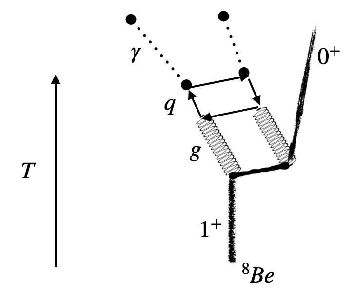
This and other scenarios remain to be investigated, but they would not be in the spirit of this paper of seeking a solution of the puzzle within the established models of nuclear physics.
II.8 Comments
The above result deserves some comments.
- •
Complete model of :
In order to go beyond the presented relations one needs a complete modeling of the excited states and their transitions. For example, the classical multipole formula (4), is a first approximation to the underlying quantum processes Buck:1977zz; Langanke:1986zz; Baye:1992nhf; Wiringa:2000gb; Pieper:2004qw; Datar:2004sx; Pastore:2014oda; Hammer:2019poc. There are also no strongly interacting subprocess, like the one shown in figure 5, considered. Further, from the most common nuclear model one would expect that most intermediate states at MeV would decay into another broad intermediate state at MeV. It is planned improve the understanding of these two points by using an effective field theory description for the nuclear states in the spirit of Zhang:2017zap; Fornal:2017msy; Hammer:2019poc. - •
Possible peaks at small angles:
The classical multipole formula allows also for peaks at small angles. These are likely to be invisible due to the large background at small angles (see 7). - •
Initial state at MeV:
In Krasznahorkay:2015iga an overlaping initial state at MeV is reported. As shown in figure 2, the kinematic relation (7) for this initial state would also be in agreement with the observed signal. However, as reported in Krasznahorkay:2015iga, no unusual excess is observed in the angular distribution of the lepton pairs originating from the MeV initial state. A possible explanation for this could be that, in addition to the with of the intermediate state , the entire MBH reaction needs to occur at a small time window . Since the width of the MeV initial state is by a factor of 14 smaller than the width of the width of the MeV initial state, this could lead to a suppression of the MBH transition for the former. - •
A smoking gun:
Very few highly energetic s are converted to electron-positron pairs through the MBH process. The conversion probability can be estimated from (13). This turns out to be if the order of . Thus, most s leave the nucleus without conversion. Measuring their angular distribution would provide a smoking gun signal for the MBH process. - •
There is another experimental result with a peak at about Krasznahorkay:2019lyl. It would be nice to offer a simultaneous explanation for both of these experiments. This is, not possible with the MBH idea, since there is no known intermediate state with the desired properties of excited Helium. However, it has been questioned that both results originate from the same physical process Siegel:2019 because they appear at different relative angle .
III Conclusion
This paper explored a new possibility of explaining the observed X17 anomaly reported in Krasznahorkay:2015iga. The study focused on a modified Bethe-Heitler transition, depicted in figure 1. For this process, one needs to consider a broad intermediate nuclear resonance and standard conservation of energy and momentum (7). The intermediate resonance is provided by the state with a large width of MeV at MeV above the ground state. Even though one finds an almost perfect agreement with the kinematic relation (7), there sere several aspects which make it unlikely that the “X17” anomaly can be explained by rates arising from the simple processes mentioned above. This is the main result of this paper, which is summarized in the table in figure 6

The idea of this work was to find a convincing explanation of the “X17” results with a modified Bethe-Heitler process. However, the answer turned out to be most likely negative, unless one can come up with some effect which considerably enhances the corresponding emission and transition probabilities. A simple direct test the hypothesis of this paper could be made by measuring the angular distribution in the two final state.
IV Acknowledgements
Many thanks to J. Schaffner-Bielich, H. Stoecker, C. Greiner, A. Hoang, H. Skarke, P. Arias, V. Datar, and C. Diaz for helpful remarks. Thanks to several colleagues from nuclear physics, for insisting on the issue with emission and conversion probabilites. This work was supported by Fondecyt 1181694.
Appendix I: Data fit
By using WebDigit one can extract information on the angular distributions of the electron-positron pairs reported in Krasznahorkay:2015iga, as shown in figure 7.


This distribution is fitted by a Gaussian
peaked at the angle
with a halfwidth
| (15) |
With a statistical error of .
Appendix II: Derivations
A: Kinematic relation 7
Given the initial nucleus and the first photon four momentum , the four momentum of the intermediate nuclear state is
| (16) |
Here, the axes was aligned with the direction of the first photon. The invariant mass square of the intermediate state is
| (17) |
where is the mass difference between the initial and the intermediate nuclear state. Inserting (16) in (17) one can solve for the first photon energy
| (18) |
The second photon can pick up an additional spatial direction which can, for convenience be chosen as the direction . The four momentum of the final nuclear state is
| (19) |
The invariant mass square of the final nuclear state is
| (20) |
where is the rest mass difference between the intermediate and the final nuclear states. Inserting (19) in (20) one can solve for the first photon energy
| (21) |
With this, the invariant mass square of the final photon state is
| (22) | |||||
| (23) |
For this simplifies to
| (24) |
as given in (7).
References
- (1) W. Heisenberg, Z. Phys. 90, no. 3-4, 209 (1934) Erratum: [Z. Phys. 92, no. 9-10, 692 (1934)]. doi:10.1007/BF01340782, 10.1007/978-3-642-70078-1 6, 10.1007/978-3-642-70078-1 8, 10.1007/BF01333516
- (2) F. Sauter, Z. Phys. 69, 742 (1931). doi:10.1007/BF01339461
- (3) W. Heisenberg and H. Euler, Z. Phys. 98, no. 11-12, 714 (1936) doi:10.1007/BF01343663, 10.1007/978-3-642-70078-1 9 [physics/0605038].
- (4) J. S. Schwinger, Phys. Rev. 82, 664 (1951). doi:10.1103/PhysRev.82.664
- (5) D. L. Burke et al., Phys. Rev. Lett. 79, 1626 (1997). doi:10.1103/PhysRevLett.79.1626
- (6) C. Bamber et al., Phys. Rev. D 60, 092004 (1999). doi:10.1103/PhysRevD.60.092004
- (7) G. A. Mourou, T. Tajima and S. V. Bulanov, Rev. Mod. Phys. 78, 309 (2006). doi:10.1103/RevModPhys.78.309
- (8) M. Marklund and P. K. Shukla, Rev. Mod. Phys. 78, 591 (2006) doi:10.1103/RevModPhys.78.591 [hep-ph/0602123].
- (9) A. Abulencia et al. [CDF Collaboration], Phys. Rev. Lett. 98, 112001 (2007) doi:10.1103/PhysRevLett.98.112001 [hep-ex/0611040].
- (10) A. R. Bell and J. G. Kirk, Phys. Rev. Lett. 101, 200403 (2008). doi:10.1103/PhysRevLett.101.200403
- (11) R. Schutzhold, H. Gies and G. Dunne, Phys. Rev. Lett. 101, 130404 (2008) doi:10.1103/PhysRevLett.101.130404 [arXiv:0807.0754 [hep-th]].
- (12) R. Ruffini, G. Vereshchagin and S. S. Xue, Phys. Rept. 487, 1 (2010) doi:10.1016/j.physrep.2009.10.004 [arXiv:0910.0974 [astro-ph.HE]].
- (13) T. Aaltonen et al. [CDF Collaboration], Phys. Rev. Lett. 102, 242001 (2009) doi:10.1103/PhysRevLett.102.242001 [arXiv:0902.1271 [hep-ex]].
- (14) A. Di Piazza, C. Muller, K. Z. Hatsagortsyan and C. H. Keitel, Rev. Mod. Phys. 84, 1177 (2012) doi:10.1103/RevModPhys.84.1177 [arXiv:1111.3886 [hep-ph]].
- (15) M. Aaboud et al. [ATLAS Collaboration], Nature Phys. 13, no. 9, 852 (2017) doi:10.1038/nphys4208 [arXiv:1702.01625 [hep-ex]].
- (16) A. J. Krasznahorkay et al., Phys. Rev. Lett. 116, no. 4, 042501 (2016) doi:10.1103/PhysRevLett.116.042501 [arXiv:1504.01527 [nucl-ex]].
- (17) A. J. Krasznahorkay et al., arXiv:1910.10459 [nucl-ex].
- (18) H. Bethe and W. Heitler, Proc. Roy. Soc. Lond. A 146, 83 (1934). doi:10.1098/rspa.1934.0140
- (19) G. K. Horton, Proc Phys. Soc. 61 3, 296 Corrections to 1948 Proc. Phys. Soc. 60 457,. (1948)
- (20) M. E. Rose, Phys. Rev. 76, 678 (1949) Erratum: [Phys. Rev. 78, 184 (1950)]. doi:10.1103/PhysRev.76.678, 10.1103/PhysRev.78.184
- (21) A. Blinne, arXiv:1701.00743 [physics.plasm-ph].
- (22) C. Hofmann, J. Reinhardt, W. Greiner, P. Schluter and G. Soff, Phys. Rev. C 42, 2632 (1990). doi:10.1103/PhysRevC.42.2632
- (23) X. Zhang and G. A. Miller, Phys. Lett. B 773, 159 (2017) doi:10.1016/j.physletb.2017.08.013 [arXiv:1703.04588 [nucl-th]].
- (24) J. L. Feng, B. Fornal, I. Galon, S. Gardner, J. Smolinsky, T. M. P. Tait and P. Tanedo, Phys. Rev. Lett. 117, no. 7, 071803 (2016) doi:10.1103/PhysRevLett.117.071803 [arXiv:1604.07411 [hep-ph]].
- (25) J. L. Feng, B. Fornal, I. Galon, S. Gardner, J. Smolinsky, T. M. P. Tait and P. Tanedo, Phys. Rev. D 95, no. 3, 035017 (2017) doi:10.1103/PhysRevD.95.035017 [arXiv:1608.03591 [hep-ph]].
- (26) P. H. Gu and X. G. He, Nucl. Phys. B 919, 209 (2017) doi:10.1016/j.nuclphysb.2017.03.023 [arXiv:1606.05171 [hep-ph]].
- (27) P. Fayet, Eur. Phys. J. C 77, no. 1, 53 (2017) doi:10.1140/epjc/s10052-016-4568-9 [arXiv:1611.05357 [hep-ph]].
- (28) M. J. Neves and J. A. Helayel Neto, Annalen Phys. 530, no. 3, 1700112 (2018) doi:10.1002/andp.201700112 [arXiv:1609.08471 [hep-ph]].
- (29) Y. Kahn, G. Krnjaic, S. Mishra-Sharma and T. M. P. Tait, JHEP 1705, 002 (2017) doi:10.1007/JHEP05(2017)002 [arXiv:1609.09072 [hep-ph]].
- (30) J. A. Dror, R. Lasenby and M. Pospelov, Phys. Rev. D 96, no. 7, 075036 (2017) doi:10.1103/PhysRevD.96.075036 [arXiv:1707.01503 [hep-ph]].
- (31) J. Kozaczuk, Phys. Rev. D 97, no. 1, 015014 (2018) doi:10.1103/PhysRevD.97.015014 [arXiv:1708.06349 [hep-ph]].
- (32) L. Delle Rose, S. Khalil and S. Moretti, Phys. Rev. D 96, no. 11, 115024 (2017) doi:10.1103/PhysRevD.96.115024 [arXiv:1704.03436 [hep-ph]].
- (33) B. Pulice, arXiv:1911.10482 [hep-ph].
- (34) J. Alexander et al., arXiv:1608.08632 [hep-ph].
- (35) U. Ellwanger and S. Moretti, JHEP 1611, 039 (2016) doi:10.1007/JHEP11(2016)039 [arXiv:1609.01669 [hep-ph]].
- (36) T. Kitahara and Y. Yamamoto, Phys. Rev. D 95, no. 1, 015008 (2017) doi:10.1103/PhysRevD.95.015008 [arXiv:1609.01605 [hep-ph]].
- (37) J. Kozaczuk, D. E. Morrissey and S. R. Stroberg, Phys. Rev. D 95, no. 11, 115024 (2017) doi:10.1103/PhysRevD.95.115024 [arXiv:1612.01525 [hep-ph]].
- (38) L. B. Jia and X. Q. Li, Eur. Phys. J. C 76, no. 12, 706 (2016) doi:10.1140/epjc/s10052-016-4561-3 [arXiv:1608.05443 [hep-ph]].
- (39) C. S. Chen, G. L. Lin, Y. H. Lin and F. Xu, Int. J. Mod. Phys. A 32, no. 31, 1750178 (2017) doi:10.1142/S0217751X17501780 [arXiv:1609.07198 [hep-ph]].
- (40) Y. Liang, L. B. Chen and C. F. Qiao, Chin. Phys. C 41, no. 6, 063105 (2017) doi:10.1088/1674-1137/41/6/063105 [arXiv:1607.08309 [hep-ph]].
- (41) M. Battaglieri et al., arXiv:1707.04591 [hep-ph].
- (42) J. A. Dror, R. Lasenby and M. Pospelov, Phys. Rev. Lett. 119, no. 14, 141803 (2017) doi:10.1103/PhysRevLett.119.141803 [arXiv:1705.06726 [hep-ph]].
- (43) A. J. Krasznahorkay et al., EPJ Web Conf. 142, 01019 (2017). doi:10.1051/epjconf/201714201019
- (44) L. Delle Rose, S. Khalil, S. J. D. King and S. Moretti, Front. in Phys. 7, 73 (2019) doi:10.3389/fphy.2019.00073 [arXiv:1812.05497 [hep-ph]].
- (45) M. Bauer, M. Neubert and A. Thamm, JHEP 1712, 044 (2017) doi:10.1007/JHEP12(2017)044 [arXiv:1708.00443 [hep-ph]].
- (46) D. S. M. Alves and N. Weiner, JHEP 1807, 092 (2018) doi:10.1007/JHEP07(2018)092 [arXiv:1710.03764 [hep-ph]].
- (47) B. Fornal, Int. J. Mod. Phys. A 32, 1730020 (2017) doi:10.1142/S0217751X17300204 [arXiv:1707.09749 [hep-ph]].
- (48) A. Denig, EPJ Web Conf. 130, 01005 (2016). doi:10.1051/epjconf/201613001005
- (49) The ATLAS collaboration [ATLAS Collaboration], ATLAS-CONF-2016-042.
- (50) I. Alikhanov and E. A. Paschos, Phys. Rev. D 97, no. 11, 115004 (2018) doi:10.1103/PhysRevD.97.115004 [arXiv:1710.10131 [hep-ph]].
- (51) L. B. Chen, Y. Liang and C. F. Qiao, arXiv:1607.03970 [hep-ph].
- (52) V. Kozhuharov, EPJ Web Conf. 142, 01018 (2017). doi:10.1051/epjconf/201714201018
- (53) E. Nardi, C. D. R. Carvajal, A. Ghoshal, D. Meloni and M. Raggi, Phys. Rev. D 97, no. 9, 095004 (2018) doi:10.1103/PhysRevD.97.095004 [arXiv:1802.04756 [hep-ph]].
- (54) D. Banerjee et al. [NA64 Collaboration], Phys. Rev. Lett. 120, no. 23, 231802 (2018) doi:10.1103/PhysRevLett.120.231802 [arXiv:1803.07748 [hep-ex]].
- (55) L. Marsicano et al., Phys. Rev. D 98, no. 1, 015031 (2018) doi:10.1103/PhysRevD.98.015031 [arXiv:1802.03794 [hep-ex]].
- (56) C. Taruggi [PADME Collaboration], “Searching for dark Photons with the PADME Experiment,”
- (57) V. Kozhuharov, EPJ Web Conf. 212, 06001 (2019). doi:10.1051/epjconf/201921206001
- (58) J. D. Jackson http://cdsweb.cern.ch/record/490457 (1999).
- (59) Ankit Rohatgi; https://automeris.io/WebPlotDigitizer.
- (60) Sukhoruchkin, & Soroko(2008)]2008LanB..19C…55S Sukhoruchkin, S. I., & Soroko, Z. N. 2008, Landolt Börnstein, 19C, 55.
- (61) T. Hahn, Comput. Phys. Commun. 140 (2001), 418-431 doi:10.1016/S0010-4655(01)00290-9 [arXiv:hep-ph/0012260 [hep-ph]].
- (62) B. Buck, H. Friedrich and C. Wheatley, Nucl. Phys. A 275, 246 (1977). doi:10.1016/0375-9474(77)90287-1
- (63) K. Langanke and C. Rolfs, Phys. Rev. C 33, 790 (1986). doi:10.1103/PhysRevC.33.790
- (64) D. Baye, P. Descouvemont and M. Kruglanski, Nucl. Phys. A 550, 250-262 (1992) doi:10.1016/0375-9474(92)90682-A
- (65) R. B. Wiringa, S. C. Pieper, J. Carlson and V. R. Pandharipande, Phys. Rev. C 62, 014001 (2000) doi:10.1103/PhysRevC.62.014001 [nucl-th/0002022].
- (66) S. C. Pieper, R. B. Wiringa and J. Carlson, Phys. Rev. C 70, 054325 (2004) doi:10.1103/PhysRevC.70.054325 [nucl-th/0409012].
- (67) V. M. Datar, S. Kumar, D. R. Chakrabarty, V. Nanal, E. T. Mirgule, A. Mitra and H. H. Oza, Phys. Rev. Lett. 94, 122502 (2005) Erratum: [Phys. Rev. Lett. 94, 139902 (2005)] doi:10.1103/PhysRevLett.94.122502, 10.1103/PhysRevLett.94.139902 [nucl-ex/0409025].
- (68) S. Pastore, R. B. Wiringa, S. C. Pieper and R. Schiavilla, Phys. Rev. C 90, no. 2, 024321 (2014) doi:10.1103/PhysRevC.90.024321 [arXiv:1406.2343 [nucl-th]].
- (69) H.-W. Hammer, S. Konig and U. van Kolck, arXiv:1906.12122 [nucl-th].
- (70) E. Siegel, Forbes science section, 26.11.2019.