跳到论文正文
W Papers独立论文阅读器 arXiv:2003.05512 论文正文 计算阅读时间 · 0%
引用这篇论文根据当前论文元数据生成,正式投稿前建议核对。


License: arXiv.org perpetual non-exclusive license
arXiv:2003.05512v2 [math.OC] 16 Oct 2020

Mechanistic Modeling of Longitudinal Shape Changes: equations of motion and inverse problemsThanks: LY was partially supported by NIH R01DC016784 and NIH U19AG033655; NC was partially supported by NSF 1912030 and NSF 1945224.

Dai-Ni Hsieh†, Sylvain Arguillère‡, Nicolas Charon†, and Laurent Younes† Address: †Department of Applied Mathematics and Statistics, Johns Hopkins University Address: ‡Laboratoire Paul Painlevé, Université de Lille Email address: dnhsieh@jhu.edu Email address: sylvain.arguillere@univ-lille.fr Email address: charon@cis.jhu.edu and Email address: laurent.younes@jhu.edu
Abstract.

This paper examines a longitudinal shape evolution model in which a 3D volume progresses through a family of elastic equilibria in response to the time-derivative of an internal force, or yank, with an additional regularization to ensure diffeomorphic transformations. We consider two different models of yank and address the long time existence and uniqueness of solutions for the equations of motion in both models. In addition, we derive sufficient conditions for the existence of an optimal yank that best describes the change from an observed initial volume to an observed volume at a later time. The main motivation for this work is the understanding of processes such as growth and atrophy in anatomical structures, where the yank could be roughly interpreted as a metabolic event triggering morphological changes. We provide preliminary results on simple examples to illustrate, under this model, the retrievability of some attributes of such events.

1. Introduction

We analyze in this paper a shape evolution paradigm introduced in [18] in which a volume progresses along a family of regularized elastic equilibria controlled by the gradient of a time-dependent potential, this gradient being interpreted as the time-derivative of an internal force that we will refer to as “yank”, following, e.g., [20]. A primary motivation of our work is the modeling of shape changes in anatomical structures, where the driving potential may be loosely interpreted as a result of metabolic events, for example, caused by a disease in the structure. Potential applications of this framework include biological growth models [13, 22, 2, 30, 16] or longitudinal studies in computational anatomy, and in particular, slow changes in the brain resulting from neuro-degenerative diseases [7, 8, 5, 26, 19, 21, 29, 15, 1, 37, 31, 35]. Such processes of pathogenesis are not well understood today. Thus we introduce a general framework under which more advanced models can be developed. In our experiments, we make very simple assumptions on the initiation and propagation of the potential. We then illustrate the possibility of inferring the causes of the shape changes only from geometric observations.

The relationship between shape and yank in our model can be represented as a control system in which the velocity field at a given time is obtained as the solution of a linear equation that depends on both. We will provide conditions ensuring that this control system has a unique solution over an arbitrary time interval before formulating and studying the inverse problem of estimating an optimal yank based only on observed initial and final shapes. We will consider two situations in this context. In the first model, we will assume that the yank is unspecified at all times. We will then estimate the yank so that it minimizes a cost accumulating over time, resulting in an optimal control problem. In the second one, the assumption will be that the potential specifying the yank is fully characterized by its initial value and follows the shape transformation through basic advection. In this latter case, we will attempt to solve the inverse problem of determining this initial value (specified by a few parameters) based on partial information on the deformation, namely the boundary of the transformed volume.

The overall paradigm defining the dynamical system is the same as that described in [18], where we assume that, at time tt, an infinitesimal force δ​F​(t)\delta F(t) is applied to a volume M⁡(t)M(t) in a zero-stress state, resulting in a new equilibrium at time t+δ​tt+\delta t, denoted by M⁡(t+δ​t)M(t+\delta t), where δ​t\delta t is small, therefore assuming that times needed to reach new equilibria are negligible compared to the time frame within which the whole process is considered. (Such an assumption of evolving reference configuration is typical in morphoelastic growth models [32, 13, 17].) The new configuration M⁡(t+δ​t)M(t+\delta t) is obtained by displacing each point xx in M⁡(t)M(t) by a small vector δ​x\delta x, which is obtained by solving a linear equation ℒ⁡(t)​δ​x=δ​F​(t)\mathcal{L}(t)\delta x=\delta F(t), where ℒ\mathcal{L} typically depends on MM. Dividing by δ​t\delta t, introducing the velocity v=δ​x/δ​tv=\delta x/\delta t and the yank j=δ​F/δ​tj=\delta F/\delta t, we are led to consider shape evolution processes in which MM is advected by the vector field vv as the solution of ℒ⁡(t)​v=j\mathcal{L}(t)v=j. The existence of solutions of such a process is stated in Theorems 1 and 2 under some assumptions on the operator ℒ\mathcal{L} (which are satisfied, in particular, by properly regularized elastic operators) and on the yank jj. Existence of solutions to the inverse problem of estimating jj from the initial and final shapes are provided in the same theorems.

The paper is organized as follows. Notation and a general description of our framework are provided in Section 2. Our main theorems are stated in Section 3 and proved in Section 6. Section 4 provides specific examples to which our theorems apply. Section 5 presents experimental results. We conclude with a discussion in Section 7 and provide implementation details in Appendix A.

2. Formulation of problems

2.1. Notation

For an integer s≥0s\geq 0, we let C0s​(ℝ3,ℝ3)C_{0}^{s}(\mathbb{R}^{3},\mathbb{R}^{3}) denote the space of ss-times continuously differentiable vector fields vv such that the kkth derivative Dk​vD^{k}v tends to 0 at infinity for every k≤sk\leq s. The space C0s​(ℝ3,ℝ3)C_{0}^{s}(\mathbb{R}^{3},\mathbb{R}^{3}) is a Banach space equipped with the norm ‖v‖s,∞=∑k=0smaxx∈ℝ3⁡|Dk​v​(x)|\|v\|_{s,\infty}=\sum_{k=0}^{s}\max_{x\,\in\,\mathbb{R}^{3}}|D^{k}v(x)|, where |⋅||\cdot| denotes the operator norm of a multilinear map on a product of finite-dimensional vector spaces equipped with the Euclidean norm. If s=0s=0, we will write the customary ‖v‖∞\|v\|_{\infty} instead of ‖v‖0,∞\|v\|_{0,\infty}.

Let 𝑖𝑑:ℝ3→ℝ3\mathit{id}:\mathbb{R}^{3}\rightarrow\mathbb{R}^{3} be the identity map, i.e., 𝑖𝑑⁡(x)=x\mathit{id}(x)=x. We denote by 𝐷𝑖𝑓𝑓𝑖𝑑s​(ℝ3)\mathit{Diff}_{\!\mathit{id}}^{s}(\mathbb{R}^{3}) the set of CsC^{s} diffeomorphisms on ℝ3{\mathbb{R}}^{3} that tend to identity at infinity. Thus every element φ∈𝐷𝑖𝑓𝑓𝑖𝑑s​(ℝ3)\varphi\in\mathit{Diff}_{\!\mathit{id}}^{s}(\mathbb{R}^{3}) can be written as φ=𝑖𝑑+v\varphi=\mathit{id}+v, where v∈C0s​(ℝ3,ℝ3)v\in C_{0}^{s}(\mathbb{R}^{3},\mathbb{R}^{3}). The affine Banach space 𝑖𝑑+C0s​(ℝ3,ℝ3)\mathit{id}+C_{0}^{s}(\mathbb{R}^{3},\mathbb{R}^{3}) is equipped with the induced metric d⁡(φ,ψ)=‖φ−ψ‖s,∞d(\varphi,\psi)=\|\varphi-\psi\|_{s,\infty}, which makes 𝐷𝑖𝑓𝑓𝑖𝑑s​(ℝ3)⊂𝑖𝑑+C0s​(ℝ3,ℝ3)\mathit{Diff}_{\!\mathit{id}}^{s}({\mathbb{R}}^{3})\subset\mathit{id}+C_{0}^{s}(\mathbb{R}^{3},\mathbb{R}^{3}) an open subset.

We will denote by ℒ⁡(B,B~)\mathscr{L}(B,\widetilde{B}) the vector space of bounded linear operators from a Banach space BB to another Banach space B~\widetilde{B}. Weak convergence of sequences (xn)(x_{n}) in BB will be denoted by xn⇀xx_{n}\rightharpoonup x. Denoting the topological dual of BB by B∗B^{*}, we will use the notation (μ|v)(\mu\,|\,v) rather than μ⁡(v)\mu(v) to denote the evaluation of μ∈B∗\mu\in B^{*} at v∈Bv\in B. We say a linear operator A∈ℒ⁡(B,B∗)A\in\mathscr{L}(B,B^{*}) is symmetric if the corresponding bilinear form (v,w)↦(A​v|w)(v,w)\mapsto(Av\,|\,w) is symmetric. The subspace of symmetric linear operators will be denoted by ℒsym​(B,B∗)\mathscr{L}_{\mathrm{sym}}(B,B^{*}).

For a generic function f:[0,T]×ℝ3→ℝ3f:[0,T]\times\mathbb{R}^{3}\rightarrow\mathbb{R}^{3}, we will use the notation f⁡(t):ℝ3→ℝ3f(t):\mathbb{R}^{3}\rightarrow\mathbb{R}^{3} defined by f​(t)​(x)=f​(t,x)f(t)(x)=f(t,x). We will use CC to denote a generic constant and CaC_{a} to show a generic constant depending on aa. The value of such constants may change from equation to equation.

Throughout this paper, VV is a separable Hilbert space of vector fields on ℝ3{\mathbb{R}}^{3} continuously embedded in C02​(ℝ3,ℝ3)C_{0}^{2}(\mathbb{R}^{3},\mathbb{R}^{3}), which is denoted by V↪C02​(ℝ3,ℝ3)V\hookrightarrow C_{0}^{2}(\mathbb{R}^{3},\mathbb{R}^{3}), with inner product ⟨⋅,⋅⟩V{\left\langle{\cdot}\,,\,{\cdot}\right\rangle}_{V} and norm ∥⋅∥V\|\cdot\|_{V}. Since V↪C02​(ℝ3,ℝ3)V\hookrightarrow C_{0}^{2}(\mathbb{R}^{3},\mathbb{R}^{3}), there exists a constant cVc_{V} such that ‖v‖2,∞≤cV​‖v‖V\|v\|_{2,\infty}\leq c_{V}\|v\|_{V}. The duality map LV:V→V∗L_{V}:V\to V^{*} is given by

(LV​v|w)=⟨v,w⟩V(L_{V}\hskip 1.0ptv\,|\,w)={\left\langle{v}\,,\,{w}\right\rangle}_{V}

and provides an isometry from VV onto V∗V^{*}. We denote the inverse of LVL_{V} by KV∈ℒ⁡(V∗,V)K_{V}\in\mathscr{L}(V^{*},V), which, because of the embedding assumption, is a kernel operator [4]. Note that

‖v‖V2=(LV​v|v)=(KV−1​v|v).\|v\|_{V}^{2}=(L_{V}\hskip 1.0ptv\,|\,v)=(K_{V}^{-1}\hskip 1.0ptv\,|\,v).

As an example, the space VV can be the reproducing kernel Hilbert space (RKHS) associated with a Matérn kernel of some order rr, and some width σ\sigma, which, in three dimensions, implies that VV is a Sobolev space Hr+2H^{r+2}. For the specific value r=3r=3, which we will use in our experiments, the kernel operator (when applied to a vector measure μ∈V∗\mu\in V^{*}) takes the form

(KV​μ)​(x)=∫ℝ3κ⁡(|x−y|/σ)​𝑑μ​(y)(K_{V}\hskip 1.0pt\mu)(x)=\int_{{\mathbb{R}}^{3}}\kappa(|x-y|/\sigma)\,d\mu(y)

with κ⁡(t)=(1+t+2​t2/15+t3/15)​e−t\kappa(t)=(1+t+2t^{2}/15+t^{3}/15)e^{-t}.

If BB is a Banach space and p≥1p\geq 1, Lp​([0,T],B)L^{p}([0,T],B) denotes the space of Bochner integrable functions f:[0,T]→Bf:[0,T]\to B such that ∫0T‖f⁡(t)‖Bp​𝑑t<∞\int_{0}^{T}\|f(t)\|_{B}^{p}\,dt<\infty. Recall that a function f:[0,T]→Bf:[0,T]\to B is Bochner integrable if: (i) it is the almost-everywhere limit of a sequence of measurable functions that take a finite number of values (also called simple functions) and (ii) satisfies ∫0T‖f⁡(t)‖B​𝑑t<∞\int_{0}^{T}\|f(t)\|_{B}\,dt<\infty.

2.2. Control systems and inverse problems

We now describe the dynamics we consider in this paper, which gradually deform shapes through elastic equilibria. We assume a mapping A:𝐷𝑖𝑓𝑓𝑖𝑑1​(ℝ3)→ℒsym​(V,V∗)A:\mathit{Diff}_{\!\mathit{id}}^{1}(\mathbb{R}^{3})\rightarrow\mathscr{L}_{\mathrm{sym}}(V,V^{*}) defined by φ↦Aφ\varphi\mapsto A_{\varphi}. Given a time-dependent mapping j:[0,T]→V∗j:[0,T]\rightarrow V^{*}, we model the deformation trajectory of a compact subset M0⊂ℝ3M_{0}\subset\mathbb{R}^{3} as t↦φj​(t,M0)t\mapsto\varphi_{j}(t,M_{0}), where φj∈C⁡([0,T],𝐷𝑖𝑓𝑓𝑖𝑑1​(ℝ3))\varphi_{j}\in C([0,T],\mathit{Diff}_{\!\mathit{id}}^{1}({\mathbb{R}}^{3})) is a solution to the system

(1) {∂tφ(t,x)=v(t,φ(t,x)),φ(0,x)=x,v⁡(t)=arg⁡minv′∈V​ω2​‖v′‖V2+12​(Aφ⁡(t)​v′|v′)−(j⁡(t)|v′)\left\{\begin{array}[]{l}\partial_{t}\hskip 1.0pt\varphi(t,x)=v(t,\varphi(t,x)),\ \varphi(0,x)=x,\\[5.0pt] \displaystyle v(t)=\underset{v^{\prime}\,\in\,V}{\arg\min}\ \frac{\omega}{2}\,\|v^{\prime}\|_{V}^{2}+\frac{1}{2}\,(A_{\varphi(t)}\hskip 1.0ptv^{\prime}\,|\,v^{\prime})-(j(t)\,|\,v^{\prime})\end{array}\right.

and ω>0\omega>0 is a fixed regularization parameter. The first equation in this system will be seen as an ordinary differential equation in 𝐷𝑖𝑓𝑓𝑖𝑑1​(ℝ3)\mathit{Diff}_{\!\mathit{id}}^{1}({\mathbb{R}}^{3}). We can interpret the squared norm ω2​‖v′‖V2\frac{\omega}{2}\,\|v^{\prime}\|_{V}^{2} as a regularization term that is introduced to ensure that v⁡(t)v(t) and (as we will see in our results) φ⁡(t)−𝑖𝑑\varphi(t)-\mathit{id} are both in C02​(ℝ2,ℝ2)C^{2}_{0}({\mathbb{R}}^{2},{\mathbb{R}}^{2}). This term will also ensure that φ⁡(t)\varphi(t) is a diffeomorphism at all times (similar regularizations were used in works such as [6, 33, 34]). The operator Aφ⁡(t)A_{\varphi(t)}, as we shall detail later, may be for instance an elastic operator in which case the second term 12​(Aφ⁡(t)​v′|v′)\frac{1}{2}\,(A_{\varphi(t)}\hskip 1.0ptv^{\prime}\,|\,v^{\prime}) represents the linear elastic energy associated to the deformation while j⁡(t)j(t) represents a yank inducing the motion of the material. In this context, the second equation in system Eq. 1 essentially states that the deformation vector field at each time is governed by an infinitesimal version of the principle of virtual work [24, Theorem 1.6, Chapter 5] with regularization. As a result, the shape φj​(t,M0)\varphi_{j}(t,M_{0}) is deformed from a stress-free state to an equilibrium at all time in this dynamical system, as described earlier in the introduction. We postpone specific examples of elastic operators and yank until Section 4, after presenting sufficient conditions ensuring existence of solutions of our inverse problems in Section 3, where we treat AφA_{\varphi} and jj as general operators.

We let ℳ\mathscr{M} denote a class of compact subsets of ℝ3{\mathbb{R}}^{3} that represents our “shape space” and assume that it is stable by the action of diffeomorphisms, i.e., φ⁡(ℳ)⊂ℳ\varphi(\mathscr{M})\subset\mathscr{M} for all φ∈𝐷𝑖𝑓𝑓𝑖𝑑1​(ℝ3)\varphi\in\mathit{Diff}_{\!\mathit{id}}^{1}(\mathbb{R}^{3}). A specific description of ℳ\mathscr{M} is problem dependent (see Remark 3). Given two elements M0,Mtarg∈ℳM_{0},M_{\mathrm{targ}}\in\mathscr{M}, providing the observed initial shape and final shape, or target, we aim to find jj within a given class such that the deformed M0M_{0} in response to jj at time TT, i.e., φj​(T,M0)\varphi_{j}(T,M_{0}), is close to MtargM_{\mathrm{targ}} in some sense. Closeness will be measured according to a discrepancy function ρ:ℳ×ℳ→[0,+∞)\rho:\mathscr{M}\times\mathscr{M}\to[0,+\infty) that compares compact sets (see examples in Remark 3). We will focus on the following two frameworks regarding the time-dependent yank jj:

  1. (1)

    Free yank model. In system Eq. 1, one can interpret jj as a control that drives the evolution of the state φ\varphi through the vector field vφv_{\varphi}. Let 𝒳V∗,Tp=Lp​([0,T],V∗)\mathcal{X}_{V^{*}\!,\,T}^{p}=L^{p}([0,T],V^{*}). We will consider the optimal control problem

    (2) min⁡∫0Tj∈𝒳V∗,T2⁡(j⁡(t)|v⁡(t))​𝑑t+ρ⁡(φ⁡(T,M0),Mtarg)\min_{j\,\in\,\mathcal{X}_{V^{*}\!,\,T}^{2}}\,\int_{0}^{T}(j(t)\,|\,v(t))\,dt+\rho(\varphi(T,M_{0}),M_{\mathrm{targ}})

    subject to system Eq. 1. We will give sufficient conditions guaranteeing the existence of solutions of this problem in Theorem 1.

  2. (2)

    Parametric yank model. The yank is modeled as a function of a transformation φ\varphi and of a finite-dimensional parameter θ\theta belonging to a compact set Θ⊂ℝm\Theta\subset{\mathbb{R}}^{m}. In this case, the finite-dimensional optimization problem of interest is

    (3) minθ∈Θ⁡ρ⁡(φ⁡(T,M0),Mtarg)\min_{\vphantom{\rule{0.0pt}{6.5pt}}\theta\,\in\,\Theta}\ \rho(\varphi(T,M_{0}),M_{\mathrm{targ}})

    subject to Eq. 1 with j⁡(t)=j⁡(φ⁡(t),θ)j(t)=j({\varphi(t)},\theta), namely,

    (4) {∂tφ(t,x)=v(t,φ(t,x)),φ(0,x)=x,v⁡(t)=arg⁡minv′∈V​ω2​‖v′‖V2+12​(Aφ⁡(t)​v′|v′)−(j⁡(φ⁡(t),θ)|v′).\left\{\begin{array}[]{ll}\partial_{t}\hskip 1.0pt\varphi(t,x)=v(t,\varphi(t,x)),\ \varphi(0,x)=x,\\[5.0pt] \displaystyle v(t)=\underset{v^{\prime}\,\in\,V}{\arg\min}\ \frac{\omega}{2}\,\|v^{\prime}\|_{V}^{2}+\frac{1}{2}\,(A_{\varphi(t)}\hskip 1.0ptv^{\prime}\,|\,v^{\prime})-(j({\varphi(t)},\theta)\,|\,v^{\prime}).\end{array}\right.

    Examples of such yanks are provided in Section 4. We give sufficient conditions for this optimization problem to have a solution in Theorem 2.

3. Main results

Given a compact subset Ω⊂ℝ3\varOmega\subset\mathbb{R}^{3}, we define the seminorm

‖v‖s,∞Ω=∑k=1smaxx∈Ω⁡|Dk​v​(x)|\|v\|_{s,\infty}^{\varOmega}=\sum_{k=1}^{s}\max_{x\,\in\,\varOmega}\,|D^{k}v(x)|

on Cs​(ℝ3,ℝ3)C^{s}(\mathbb{R}^{3},\mathbb{R}^{3}). We require a regularity assumption on the discrepancy function ρ\rho appearing in the objective functionals Eqs. 2 and 3.

Definition 1.

We say that a discrepancy function ρ:ℳ×ℳ→[0,+∞)\rho:\mathscr{M}\times\mathscr{M}\to[0,+\infty) is continuous on ℳ\mathscr{M} with respect to ∥⋅∥s,∞\|\cdot\|_{s,\infty} if for all compact sets M,M′∈ℳM,M^{\prime}\in\mathscr{M} and all sequences (φn)n=1∞⊂𝐷𝑖𝑓𝑓𝑖𝑑s​(ℝ3)(\varphi_{n})_{n=1}^{\infty}\subset\mathit{Diff}_{\!\mathit{id}}^{s}({\mathbb{R}}^{3}) such that ‖φn−φ‖s,∞M→0\|\varphi_{n}-\varphi\|_{s,\infty}^{M}\rightarrow 0 for some φ∈𝐷𝑖𝑓𝑓𝑖𝑑s​(ℝ3)\varphi\in\mathit{Diff}_{\!\mathit{id}}^{s}({\mathbb{R}}^{3}), one has

ρ⁡(φn​(M),M′)→ρ⁡(φ⁡(M),M′).\rho(\varphi_{n}(M),M^{\prime})\rightarrow\rho(\varphi(M),M^{\prime}).
Theorem 1 (Free yank model).

Let A:𝐷𝑖𝑓𝑓𝑖𝑑1​(ℝ3)→ℒsym​(V,V∗)A:\mathit{Diff}_{\!\mathit{id}}^{1}(\mathbb{R}^{3})\rightarrow\mathscr{L}_{\mathrm{sym}}(V,V^{*}) be a mapping defined by φ↦Aφ\varphi\mapsto A_{\varphi}. Assume that (Aφ​v|v)≥0(A_{\varphi}\hskip 1.0ptv\,|\,v)\geq 0 for all φ∈𝐷𝑖𝑓𝑓𝑖𝑑1​(ℝ3)\varphi\in\mathit{Diff}_{\!\mathit{id}}^{1}(\mathbb{R}^{3}) and v∈Vv\in V. Let the two compact sets M0,Mtarg∈ℳM_{0},M_{\mathrm{targ}}\in\mathscr{M} be given. Then the following results hold.

  1. (i)

    Suppose that φ↦Aφ\varphi\mapsto A_{\varphi} is locally Lipschitz (for the ∥⋅∥1,∞\|\cdot\|_{1,\infty} distance). Then, given j∈𝒳V∗,T1j\in\mathcal{X}_{V^{*}\!,\,T}^{1}, the system

    (1) {∂tφ(t,x)=v(t,φ(t,x)),φ(0,x)=x,v⁡(t)=arg⁡minv′∈V​ω2​‖v′‖V2+12​(Aφ⁡(t)​v′|v′)−(j⁡(t)|v′).\left\{\begin{array}[]{l}\partial_{t}\hskip 1.0pt\varphi(t,x)=v(t,\varphi(t,x)),\ \varphi(0,x)=x,\\[5.0pt] \displaystyle v(t)=\underset{v^{\prime}\,\in\,V}{\arg\min}\ \frac{\omega}{2}\,\|v^{\prime}\|_{V}^{2}+\frac{1}{2}\,(A_{\varphi(t)}\hskip 1.0ptv^{\prime}\,|\,v^{\prime})-(j(t)\,|\,v^{\prime})\end{array}\right..

    has a unique solution φ∈C⁡([0,T],𝐷𝑖𝑓𝑓𝑖𝑑2​(ℝ3))\varphi\in C([0,T],\mathit{Diff}_{\!\mathit{id}}^{2}(\mathbb{R}^{3})).

  2. (ii)

    Suppose that, for each γ>0\gamma>0, the mapping φ↦Aφ\varphi\mapsto A_{\varphi} is Lipschitz with respect to the seminorm ∥⋅∥1,∞M0\|\cdot\|_{1,\infty}^{M_{0}} on

    𝔖γ={φ∈𝐷𝑖𝑓𝑓𝑖𝑑1​(ℝ3):‖φ−i​d‖1,∞≤γ​ and ​‖φ−1−i​d‖1,∞≤γ}.\mathfrak{S}_{\gamma}=\{\varphi\in\mathit{Diff}_{\!\mathit{id}}^{1}(\mathbb{R}^{3}):\|\varphi-id\|_{1,\infty}\leq\gamma\mbox{ and }\|\varphi^{-1}-id\|_{1,\infty}\leq\gamma\}.

    In addition, assume that the discrepancy function ρ\rho is continuous on ℳ\mathscr{M} with respect to ∥⋅∥1,∞\|\cdot\|_{1,\infty}. Then there exists a minimizer of the optimal control problem

    min⁡∫0Tj∈𝒳V∗,T2⁡(j⁡(t)|v⁡(t))​𝑑t+ρ⁡(φ⁡(T,M0),Mtarg)\min_{j\,\in\,\mathcal{X}_{V^{*}\!,\,T}^{2}}\,\int_{0}^{T}(j(t)\,|\,v(t))\,dt+\rho(\varphi(T,M_{0}),M_{\mathrm{targ}})

    where vv and φ\varphi satisfy Eq. 1.

Before stating our next theorem, we remind the reader that a collection of functions is said to be equi-Lipschitz if they are all Lipschitz and there exists a common Lipschitz constant that applies to all functions in the collection.

Theorem 2 (Parametric yank model).

Let A:𝐷𝑖𝑓𝑓𝑖𝑑1​(ℝ3)→ℒsym​(V,V∗)A:\mathit{Diff}_{\!\mathit{id}}^{1}(\mathbb{R}^{3})\rightarrow\mathscr{L}_{\mathrm{sym}}(V,V^{*}) be a mapping defined by φ↦Aφ\varphi\mapsto A_{\varphi}. Assume that (Aφ​v|v)≥0(A_{\varphi}\hskip 1.0ptv\,|\,v)\geq 0 for all φ∈𝐷𝑖𝑓𝑓𝑖𝑑1​(ℝ3)\varphi\in\mathit{Diff}_{\!\mathit{id}}^{1}(\mathbb{R}^{3}) and v∈Vv\in V. Moreover, let Θ⊂ℝm\Theta\subset\mathbb{R}^{m} be a compact set and let j:𝐷𝑖𝑓𝑓𝑖𝑑1​(ℝ3)×Θ→V∗j:\mathit{Diff}_{\!\mathit{id}}^{1}(\mathbb{R}^{3})\times\Theta\rightarrow V^{*}. Finally, let two compact sets M0,Mtarg∈ℳM_{0},M_{\mathrm{targ}}\in\mathscr{M} be given. Then the following results hold.

  1. (i)

    Suppose that φ↦Aφ\varphi\mapsto A_{\varphi} is locally Lipschitz and that φ↦j⁡(φ,θ)\varphi\mapsto j(\varphi,\theta) is locally Lipschitz (in both cases for ∥⋅∥1,∞\|\cdot\|_{1,\infty} distance) and bounded in norm. Given θ∈Θ\theta\in\Theta, the system

    (4) {∂tφ(t,x)=v(t,φ(t,x)),φ(0,x)=x,v⁡(t)=arg⁡minv′∈V​ω2​‖v′‖V2+12​(Aφ⁡(t)​v′|v′)−(j⁡(φ⁡(t),θ)|v′).\left\{\begin{array}[]{ll}\partial_{t}\hskip 1.0pt\varphi(t,x)=v(t,\varphi(t,x)),\ \varphi(0,x)=x,\\[5.0pt] \displaystyle v(t)=\underset{v^{\prime}\,\in\,V}{\arg\min}\ \frac{\omega}{2}\,\|v^{\prime}\|_{V}^{2}+\frac{1}{2}\,(A_{\varphi(t)}\hskip 1.0ptv^{\prime}\,|\,v^{\prime})-(j({\varphi(t)},\theta)\,|\,v^{\prime})\end{array}\right..

    has a unique solution φ∈C⁡([0,T],𝐷𝑖𝑓𝑓𝑖𝑑2​(ℝ3))\varphi\in C([0,T],\mathit{Diff}_{\!\mathit{id}}^{2}(\mathbb{R}^{3})).

  2. (ii)

    Suppose that:

    1. ∙\bullet

      For each γ>0\gamma>0, the mapping φ↦Aφ\varphi\mapsto A_{\varphi} is Lipschitz and the family of mappings {j⁡(⋅,θ):θ∈Θ}\{j(\cdot,\theta):\theta\in\Theta\} is equi-Lipschitz, both with respect to the seminorm ∥⋅∥1,∞M0\|\cdot\|_{1,\infty}^{M_{0}}, on the set

      𝔖γ={φ∈𝐷𝑖𝑓𝑓𝑖𝑑1​(ℝ3):‖φ−i​d‖1,∞≤γ​ and ​‖φ−1−i​d‖1,∞≤γ}.\mathfrak{S}_{\gamma}=\{\varphi\in\mathit{Diff}_{\!\mathit{id}}^{1}(\mathbb{R}^{3}):\|\varphi-id\|_{1,\infty}\leq\gamma\mbox{ and }\|\varphi^{-1}-id\|_{1,\infty}\leq\gamma\}.
    2. ∙\bullet

      For all φ∈𝐷𝑖𝑓𝑓𝑖𝑑1​(ℝ3)\varphi\in\mathit{Diff}_{\!\mathit{id}}^{1}(\mathbb{R}^{3}), j⁡(φ,⋅)j(\varphi,\cdot) is continuous in the sense that

      θn→θ implies j⁡(φ,θn)⇀j⁡(φ,θ).\theta_{n}\rightarrow\theta\ \ \mbox{ implies }\ \ j(\varphi,\theta_{n})\rightharpoonup j(\varphi,\theta).
    3. ∙\bullet

      There exists a constant JΘJ_{\Theta} such that

      ‖j⁡(φ,θ)‖V∗≤JΘ for all ​φ∈𝐷𝑖𝑓𝑓𝑖𝑑1​(ℝ3)​ and ​θ∈Θ.\|j(\varphi,\theta)\|_{V^{*}}\leq J_{\Theta}\ \ \mbox{ for all }\varphi\in\mathit{Diff}_{\!\mathit{id}}^{1}(\mathbb{R}^{3})\mbox{ and }\theta\in\Theta.
    4. ∙\bullet

      The discrepancy function ρ\rho is continuous on ℳ\mathscr{M} with respect to ∥⋅∥1,∞\|\cdot\|_{1,\infty}.

    Then there exists a minimizer for the finite-dimensional optimization problem

    minθ∈Θ⁡ρ⁡(φ⁡(T,M0),Mtarg)\min_{\vphantom{\rule{0.0pt}{6.5pt}}\theta\,\in\,\Theta}\ \rho(\varphi(T,M_{0}),M_{\mathrm{targ}})

    where φ\varphi satisfies Eq. 4.

We will prove these two theorems in Section 6. Both control systems can be considered as ordinary differential equations with values in the affine Banach space 𝑖𝑑+C01​(ℝd,ℝd)\mathit{id}+C_{0}^{1}({\mathbb{R}}^{d},{\mathbb{R}}^{d}). Most of the effort in proving the long-time existence and uniqueness of solutions, part (i) of the theorems, will rely on controlling the vector field v⁡(t)v(t) by the input, jj in the first case and θ\theta in the second case. A key step for this is provided by Lemma (iii), which exploits the regularization term ω2​‖v′‖V2\frac{\omega}{2}\,\|v^{\prime}\|_{V}^{2}. After this key step, we can carry out a proof using the Banach fixed point theorem and the Picard iteration in the space C⁡([0,T],𝐷𝑖𝑓𝑓𝑖𝑑1​(ℝ3))C([0,T],\mathit{Diff}_{\!\mathit{id}}^{1}(\mathbb{R}^{3})). Due to the regularity of the vector field, Lemma 3 will show that the obtained unique solution is actually in C⁡([0,T],𝐷𝑖𝑓𝑓𝑖𝑑2​(ℝ3))C([0,T],\mathit{Diff}_{\!\mathit{id}}^{2}(\mathbb{R}^{3})). For part (ii) of the theorems, we will use the direct method of calculus of variations to prove the existence of minimizers. Denoting the objective function by ff, the two key steps of the direct method are proving that a minimizing sequence is bounded and that ff is weakly sequentially lower semicontinuous. The choice of the objective function affects the first step (see Remark 2). To accomplish the second step, we need to show f⁡(j)≤lim infn→∞f⁡(jn)f(j)\leq\liminf_{n\rightarrow\infty}f(j_{n}) for any sequence jn⇀jj_{n}\rightharpoonup j. We prove this by going through an intermediate step:

jn⇀j⇒‖φjn​(t)−φj​(t)‖1,∞M0→0⇒f⁡(j)≤lim infn→∞f⁡(jn),j_{n}\rightharpoonup j\ \Rightarrow\ \|\varphi_{j_{n}}\!(t)-\varphi_{j}(t)\|_{1,\infty}^{M_{0}}\rightarrow 0\ \Rightarrow\ f(j)\leq\liminf_{n\rightarrow\infty}f(j_{n}),

where φjn\varphi_{j_{n}} and φj\varphi_{j} are solutions given jnj_{n} and jj respectively. The seminorm ∥⋅∥1,∞M0\|\cdot\|_{1,\infty}^{M_{0}} is adopted to resolve a difficulty in this intermediate step: although jn⇀jj_{n}\rightharpoonup j implies φjn​(t,x)→φj​(t,x)\varphi_{j_{n}}\!(t,x)\rightarrow\varphi_{j}(t,x) pointwise, we do note have the uniform convergence. Fortunately, the convergence in the seminorm given by the Arzelà–Ascoli theorem suffices.

Remark 1.

We stated our theorems in dimension three because it corresponds to most interesting situations in practice, but our proofs apply without change to any dimension (and we are providing some experimental illustrations in dimension two).

Remark 2.

The choice we made for the control cost (j|v)(j\,|\,v) in Theorem 1 is one among a large spectrum of costs for which the conclusions of the theorem are valid. We took this specific example for simplicity and also because it provided the best results in our experiments among some other options we tried. Other possible examples could be ‖j‖V∗2\|j\|^{2}_{V^{*}}, or ‖j‖L22\|j\|^{2}_{L^{2}}, for which our proofs can easily be modified (actually, simplified), with details being left to the reader.

Remark 3.

In the experiments presented in this paper, we will use discrepancy functions based on the varifold pseudo-metrics introduced in [11] between certain surfaces associated with the two volumes (e.g., their boundaries). In this case, ℳ\mathscr{M} is the set of all compact subsets M⊂ℝ3M\subset\mathbb{R}^{3} whose boundary ∂M\partial M is a rectifiable surface (we refer to [28] for the precise definition and properties of rectifiable sets). Then, given MM and M′M^{\prime} in ℳ\mathscr{M}, for SS and S′S^{\prime} two rectifiable surfaces extracted from MM and M′M^{\prime} (such as for instance the boundaries of the volumes or some corresponding internal layers) the discrepancy function takes the following form:

ρ⁡(M,M′)=ν⁡(S,S)−2​ν​(S,S′)+ν⁡(S′,S′)\rho(M,M^{\prime})=\nu(S,S)-2\nu(S,S^{\prime})+\nu(S^{\prime},S^{\prime})

with

ν⁡(S,S′)=∫S∫S′χ⁡(|x−x′|τ)​(n​(x)⊤​n′​(x′))2​𝑑σ​(x)​d​σ′​(x′)\nu(S,S^{\prime})=\int_{S}\int_{S^{\prime}}\chi\left(\frac{|x-x^{\prime}|}{\tau}\right)(n(x)^{\top}n^{\prime}(x^{\prime}))^{2}\,d\sigma(x)\,d\sigma^{\prime}(x^{\prime})

where σ\sigma and σ′\sigma^{\prime} are volume measures on SS and S′S^{\prime}, nn and n′n^{\prime} are unit normal vector fields of SS and S′S^{\prime} and χ\chi is some radial kernel function, scaled by a scalar τ>0\tau>0, which in our experiments is taken to be the Cauchy kernel

χ⁡(t)=(1+t2)−2.\chi(t)=(1+t^{2})^{-2}.

It can be then shown, cf., [10, Proposition 6], that such discrepancy functions are continuous on ℳ\mathscr{M} with respect to ∥⋅∥1,∞\|\cdot\|_{1,\infty}, in the sense of Definition 1.

As a side note, one could alternatively select ρ\rho as the volume of the symmetric difference between the two sets, i.e., ρ⁡(M,M′)=vol​(M△M′)\rho(M,M^{\prime})=\text{vol}(M\bigtriangleup M^{\prime}) which is continuous on compact sets with respect to ∥⋅∥0,∞\|\cdot\|_{0,\infty} and thus also with respect to ∥⋅∥1,∞\|\cdot\|_{1,\infty}, thereby satisfying the assumption of the above theorems. In this case, the shape space ℳ\mathscr{M} is composed of all compact subsets of ℝ3\mathbb{R}^{3}.

Remark 4.

A model based on principles that are similar to ours has been introduced and studied in [9] in order to model tissue growth. In [9], the second equation in system Eq. 1 is replaced by the minimization of an isotropic linear elastic energy under the constraint that div​v=g⁡(u)\mathrm{div}\,v=g(u), where gg is a fixed function and uu is the concentration of morphogen, a growth-induced chemical produced by cells. The concentration of morphogen is controlled by the density of cells via a linear elliptic equation, and the density of cells is advected under the motion. While we consider here more general elasticity models, inducing additional complications in the analysis because these elastic properties must also be advected along the flow, the main difference between the two models results from the regularization ω2​‖v′‖V2\frac{\omega}{2}\,\|v^{\prime}\|_{V}^{2} added in Eq. 1. It is this term that guarantees the regularity of the vector field vv (see Lemma 1) and allows us to prove long-time existence of solutions, while [9] only obtains local existence results. Such a property is necessary to formulate optimal control problems, which form the second focus of our paper, and could not be addressed in [9].

4. Examples of elastic operators and yank

In this section, we provide examples of elastic operators and yank that satisfy the conditions in Theorems 1 and 2. Denote the space of symmetric bilinear forms on the space of 3-by-3 symmetric matrices by Σ2​(Sym3​(ℝ),Sym3​(ℝ))\Sigma_{2}(\mathrm{Sym}_{3}(\mathbb{R}),\mathrm{Sym}_{3}(\mathbb{R})). Given φ∈𝐷𝑖𝑓𝑓𝑖𝑑1​(ℝ3)\varphi\in\mathit{Diff}_{\!\mathit{id}}^{1}(\mathbb{R}^{3}), an elastic operator Aφ∈ℒsym​(V,V∗)A_{\varphi}\in\mathscr{L}_{\mathrm{sym}}(V,V^{*}) takes the following form

(5) (Aφ​u|v)=∫φ⁡(M0)Eφ​(εu,εv)​𝑑x=∫φ⁡(M0)(Eφ​(x))​(εu​(x),εv​(x))​𝑑x,(A_{\varphi}\hskip 1.0ptu\,|\,v)=\int_{\varphi(M_{0})}E_{\varphi}(\varepsilon_{u},\varepsilon_{v})\,dx=\int_{\varphi(M_{0})}(E_{\varphi}(x))(\varepsilon_{u}(x),\varepsilon_{v}(x))\,dx,

where Eφ:φ⁡(M0)→Σ2​(Sym3​(ℝ),Sym3​(ℝ))E_{\varphi}:\varphi(M_{0})\rightarrow\Sigma_{2}(\mathrm{Sym}_{3}(\mathbb{R}),\mathrm{Sym}_{3}(\mathbb{R})) is a stiffness tensor after the shape is deformed by φ\varphi, and εu\varepsilon_{u} and εv\varepsilon_{v} are linear strain tensors defined by

εu=12​(D​u+D​u⊤) and εv=12​(D​v+D​v⊤).\varepsilon_{u}=\frac{1}{2}\left(Du+Du^{\top}\right)\ \ \mbox{ and }\ \ \varepsilon_{v}=\frac{1}{2}\left(Dv+Dv^{\top}\right).

We recall the basic assumption in our model that the deformed configuration becomes a new reference for the next infinitesimal shape changes (with material properties advected by the flow). This is reflected in equation Eq. 5.

A simple example, assuming that the elastic property of an isotropic elastic material is unaffected by deformation, or persistent, is provided by Eφ​(εu,εv)=λ​tr​(εu)​tr​(εv)+2​μ​tr​(εu⊤​εv)E_{\varphi}(\varepsilon_{u},\varepsilon_{v})=\lambda\,\mathrm{tr}(\varepsilon_{u})\,\mathrm{tr}(\varepsilon_{v})+2\mu\,\mathrm{tr}(\varepsilon_{u}^{\top}\varepsilon_{v}), where λ\lambda and μ\mu are the Lamé parameters. More generally, the following proposition proved in Section 6 provides a sufficient condition on the mapping φ↦Eφ\varphi\mapsto E_{\varphi} ensuring that the corresponding AφA_{\varphi} satisfies the conditions of Theorems 1 and 2.

Proposition 1.

Suppose that Eφ​(x)E_{\varphi}(x) is positive definite for all φ∈𝐷𝑖𝑓𝑓𝑖𝑑1​(ℝ3)\varphi\in\mathit{Diff}_{\!\mathit{id}}^{1}(\mathbb{R}^{3}) and x∈φ⁡(M0)x\in\varphi(M_{0}). Moreover, suppose that, for each γ>0\gamma>0, there exists αγ>0\alpha_{\gamma}>0 such that

(6) ∫M0|Eφ∘φ−Eψ∘ψ|​𝑑x≤αγ​‖φ−ψ‖1,∞M0 for all ​φ,ψ∈𝔖γ,\int_{M_{0}}\,|E_{\varphi}\circ\varphi-E_{\psi}\circ\psi|\,dx\leq\alpha_{\gamma}\,\|\varphi-\psi\|_{1,\infty}^{M_{0}}\ \ \mbox{ for all }\varphi,\psi\in\mathfrak{S}_{\gamma},

where

𝔖γ={φ∈𝐷𝑖𝑓𝑓𝑖𝑑1(ℝ3):∥φ−id∥1,∞≤γ and ∥φ−1−id∥1,∞≤γ.}\mathfrak{S}_{\gamma}=\{\varphi\in\mathit{Diff}_{\!\mathit{id}}^{1}(\mathbb{R}^{3}):\|\varphi-id\|_{1,\infty}\leq\gamma\mbox{ and }\|\varphi^{-1}-id\|_{1,\infty}\leq\gamma.\}

Then, for AφA_{\varphi} defined as in Eq. 5, the mapping φ↦Aφ\varphi\mapsto A_{\varphi} satisfies the conditions of Theorems 1 and 2.

Example 1.

According to Proposition 1, the simplest example of the elastic operator is when the stiffness tensor EφE_{\varphi} is constant and positive definite since the left-hand side of Eq. 6 is zero. Thus our example of persistent isotropic elastic material, i.e., Eφ​(εu,εv)=λ​tr​(εu)​tr​(εv)+2​μ​tr​(εu⊤​εv)E_{\varphi}(\varepsilon_{u},\varepsilon_{v})=\lambda\,\mathrm{tr}(\varepsilon_{u})\,\mathrm{tr}(\varepsilon_{v})+2\mu\,\mathrm{tr}(\varepsilon_{u}^{\top}\varepsilon_{v}), is a valid choice. More generally, suppose that Λ:M0→Σ2​(Sym3​(ℝ),Sym3​(ℝ))\varLambda:M_{0}\rightarrow\Sigma_{2}(\mathrm{Sym}_{3}(\mathbb{R}),\mathrm{Sym}_{3}(\mathbb{R})) and that Λ⁡(x)\varLambda(x) is positive definite for all x∈M0x\in M_{0}, then Eφ:⁣=Λ∘φ−1E_{\varphi}\mathrel{\mathchoice{\vbox{\hbox{$\displaystyle:$}}}{\vbox{\hbox{$\textstyle:$}}}{\vbox{\hbox{$\scriptstyle:$}}}{\vbox{\hbox{$\scriptscriptstyle:$}}}{=}}\varLambda\circ\varphi^{-1} also satisfies the conditions in Proposition 1. Note that this form of EφE_{\varphi} preserves the elastic properties of the material from xx to φ⁡(x)\varphi(x).

Example 2.

Even more generally, let Fφ:φ⁡(M0)→G​L​(3,ℝ)F_{\varphi}:\varphi(M_{0})\rightarrow GL(3,\mathbb{R}) be a deformation-dependent frame field, where G​L​(3,ℝ)GL(3,\mathbb{R}) denotes the general linear group. We consider stiffness tensors of the form E~φ(εu,εv):⁣=(Λ∘φ−1)(Fφ⊤εuFφ,Fφ⊤εvFφ)\widetilde{E}_{\varphi}(\varepsilon_{u},\varepsilon_{v})\mathrel{\mathchoice{\vbox{\hbox{$\displaystyle:$}}}{\vbox{\hbox{$\textstyle:$}}}{\vbox{\hbox{$\scriptstyle:$}}}{\vbox{\hbox{$\scriptscriptstyle:$}}}{=}}(\varLambda\circ\varphi^{-1})(F_{\varphi}^{\top}\varepsilon_{u}F_{\varphi},F_{\varphi}^{\top}\varepsilon_{v}F_{\varphi}), where Λ\varLambda is the same as in Example 1.

The following proposition, whose proof is elementary and left to the reader, provides sufficient conditions on FF ensuring that E~\widetilde{E} satisfies the conditions in Proposition 1. Note that in this case, the elastic properties at φ⁡(x)\varphi(x) are modified from the ones at xx through a change of the frame coordinates Fφ​(φ​(x))F_{\varphi}(\varphi(x)).

Proposition 2.

Suppose that EE satisfies the conditions in Proposition 1. Let Fφ:ℝ3→G​L​(3,ℝ)F_{\varphi}:\mathbb{R}^{3}\rightarrow GL(3,\mathbb{R}) be essentially bounded for each φ∈𝐷𝑖𝑓𝑓𝑖𝑑1​(ℝ3)\varphi\in\mathit{Diff}_{\!\mathit{id}}^{1}(\mathbb{R}^{3}). If there exists βγ>0\beta_{\gamma}>0 such that

‖Fφ∘φ−Fψ∘ψ‖∞≤βγ​‖φ−ψ‖1,∞M0 for all ​φ,ψ∈𝔖γ,\|F_{\varphi}\circ\varphi-F_{\psi}\circ\psi\|_{\infty}\leq\beta_{\gamma}\,\|\varphi-\psi\|_{1,\infty}^{M_{0}}\ \ \mbox{ for all }\varphi,\psi\in\mathfrak{S}_{\gamma},

then E~\widetilde{E} defined by E~φ​(εu,εv)=Eφ​(Fφ⊤​εu​Fφ,Fφ⊤​εv​Fφ)\widetilde{E}_{\varphi}(\varepsilon_{u},\varepsilon_{v})=E_{\varphi}(F_{\varphi}^{\top}\varepsilon_{u}F_{\varphi},F_{\varphi}^{\top}\varepsilon_{v}F_{\varphi}) also satisfies the conditions in Proposition 1.

Let w1,w2w_{1},w_{2}, and w3w_{3} be linearly independent vector fields on M0M_{0}. Examples of frame fields FφF_{\varphi} that satisfy the previous assumptions include

Fφ=[D​φ​w1|D​φ​w1|,D​φ​w2|D​φ​w2|,D​φ​w3|D​φ​w3|]∘φ−1F_{\varphi}=\left[\begin{array}[]{ccc}\displaystyle\frac{D\varphi\,w_{1}}{|D\varphi\,w_{1}|},&\displaystyle\frac{D\varphi\,w_{2}}{|D\varphi\,w_{2}|},&\displaystyle\frac{D\varphi\,w_{3}}{|D\varphi\,w_{3}|}\end{array}\right]\circ\varphi^{-1}

and

Fφ=[D​φ​w1|D​φ​w1|,(D​φ​w1×D​φ​w2)×D​φ​w1|(D​φ​w1×D​φ​w2)×D​φ​w1|,D​φ​w3|D​φ​w3|]∘φ−1.\displaystyle F_{\varphi}=\left[\begin{array}[]{ccc}\displaystyle\frac{D\varphi\,w_{1}}{|D\varphi\,w_{1}|},&\displaystyle\frac{(D\varphi\,w_{1}\times D\varphi\,w_{2})\times D\varphi\,w_{1}}{|(D\varphi\,w_{1}\times D\varphi\,w_{2})\times D\varphi\,w_{1}|},&\displaystyle\frac{D\varphi\,w_{3}}{|D\varphi\,w_{3}|}\end{array}\right]\circ\varphi^{-1}.

Note that the first two vectors of the latter FφF_{\varphi} are orthonormal for all deformation φ\varphi.

Example 3.

An elastic operator inspired by the laminar organization of the cerebral cortex using the frame field Example 2 was introduced in [18]; we describe it here for completeness. Suppose that a compact subset M0⊂ℝ3M_{0}\subset\mathbb{R}^{3} has two surfaces ℳbottom\mathcal{M}_{\mathrm{bottom}} and ℳtop\mathcal{M}_{\mathrm{top}} as bottom and top layers. Moreover, suppose that we are given a diffeomorphism Φ:[0,1]×ℳbottom→M0\varPhi:[0,1]\times\mathcal{M_{\mathrm{bottom}}}\rightarrow M_{0} such that Φ⁡(0,ℳbottom)=ℳbottom\varPhi(0,\mathcal{M_{\mathrm{bottom}}})=\mathcal{M_{\mathrm{bottom}}} and Φ⁡(1,ℳbottom)=ℳtop\varPhi(1,\mathcal{M_{\mathrm{bottom}}})=\mathcal{M_{\mathrm{top}}}. Note that Φ⁡(ν,ℳbottom)=:ℳν\varPhi(\nu,\mathcal{M_{\mathrm{bottom}}})\mathrel{{=}\mathchoice{\vbox{\hbox{$\displaystyle:$}}}{\vbox{\hbox{$\textstyle:$}}}{\vbox{\hbox{$\scriptstyle:$}}}{\vbox{\hbox{$\scriptscriptstyle:$}}}}\mathcal{M}_{\nu} is a surface for each ν∈[0,1]\nu\in[0,1]. We refer to Φ\varPhi as a layered structure of M0M_{0}. Such a structure induces a transversal vector field S:⁣=∂νΦS\mathrel{\mathchoice{\vbox{\hbox{$\displaystyle:$}}}{\vbox{\hbox{$\textstyle:$}}}{\vbox{\hbox{$\scriptstyle:$}}}{\vbox{\hbox{$\scriptscriptstyle:$}}}{=}}\partial_{\nu}\varPhi (Fig. 1). Let T1T_{1} and T2T_{2} be linearly independent vector fields on M0M_{0} such that T1​ ℳνT_{1}\,\rule[-3.0pt]{0.4pt}{8.0pt}\vphantom{T_{1}}_{\,\mathcal{M}_{\nu}} and T2​ ℳνT_{2}\,\rule[-3.0pt]{0.4pt}{8.0pt}\vphantom{T_{2}}_{\,\mathcal{M}_{\nu}} are tangent to ℳν\mathcal{M}_{\nu}. Then, T1T_{1}, T2T_{2}, and SS are linearly independent vector fields on M0M_{0}. If we let w1=T1w_{1}=T_{1}, w2=T2w_{2}=T_{2}, and w3=Sw_{3}=S in Example 2 and define

(8) Λ¯​(ε,ε)=λtan​(ε11+ε22)2+μtan​(ε112+ε222+2​ε122)+μtsv​ε332+μang​(2​ε132+2​ε232),\displaystyle\begin{split}\bar{\varLambda}(\varepsilon,\varepsilon)&=\lambda_{\mathrm{tan}}(\varepsilon_{11}+\varepsilon_{22})^{2}+\mu_{\mathrm{tan}}(\varepsilon_{11}^{2}+\varepsilon_{22}^{2}+2\varepsilon_{12}^{2})\\ &\hskip 13.0pt\phantom{}+\mu_{\mathrm{tsv}}\,\varepsilon_{33}^{2}+\mu_{\mathrm{ang}}(2\varepsilon_{13}^{2}+2\varepsilon_{23}^{2}),\end{split}

where εi​j\varepsilon_{ij} denotes the i​jijth element of ε∈Sym3​(ℝ)\varepsilon\in\mathrm{Sym}_{3}(\mathbb{R}) and λtan\lambda_{\mathrm{tan}}, μtan\mu_{\mathrm{tan}}, μtsv\mu_{\mathrm{tsv}}, and μang\mu_{\mathrm{ang}} are constants, then the corresponding elastic operator

(9) (Aφ​u|v)=∫φ⁡(M0)Λ¯​(Fφ⊤​εu​Fφ,Fφ⊤​εv​Fφ)​𝑑x\displaystyle(A_{\varphi}\hskip 1.0ptu\,|\,v)=\int_{\varphi(M_{0})}\bar{\varLambda}(F_{\varphi}^{\top}\varepsilon_{u}F_{\varphi},F_{\varphi}^{\top}\varepsilon_{v}F_{\varphi})\,dx

is well-defined [18] and a valid choice by Examples 1 and 2. Note that the layered structure on a deformed shape φ⁡(M0)\varphi(M_{0}) becomes (ν,x)↦φ∘Φ⁡(ν,φ−1​(x))(\nu,x)\mapsto\varphi\circ\varPhi(\nu,\varphi^{-1}(x)). The elastic material corresponding to this elastic operator has the property that it is isotropic along the directions tangent to the layers. Figures 2(b) and 2(c) illustrate deformations φj​(T,M0)\varphi_{j}(T,M_{0}) according to system Eq. 1 under different elastic parameters μtan\mu_{\mathrm{tan}} and μtsv\mu_{\mathrm{tsv}} when we apply the same yank jj to a layered shape M0M_{0} (Fig. 2(a)).

Figure 1. Different layered structures of the same rectangular region. Shown in the figures are top layer, one middle layer, bottom layer, and the transversal vector field.
Refer to caption
(a) A simulated layered shape.
Refer to caption
(b) Tangential deformation.
Refer to caption
(c) Transversal deformation.
Figure 2. Responses to the same yank under different layered elastic parameters. In (b), μtan=0.02​μtsv\mu_{\mathrm{tan}}=0.02\,\mu_{\mathrm{tsv}}. In (c), μtsv=0.02​μtan\mu_{\mathrm{tsv}}=0.02\,\mu_{\mathrm{tan}}.
Example 4.

Now we provide an example of yank which has a density as the gradient of a transported potential. Let Θ⊂ℝm\Theta\subset\mathbb{R}^{m} be a compact set and let g:Θ→L∞​(ℝ3,ℝ)g:\Theta\rightarrow L^{\infty}(\mathbb{R}^{3},\mathbb{R}) defined by θ↦gθ\theta\mapsto g_{\theta}. We interpret gθg_{\theta} as a parametrized potential. We assume that there exists GΘ>0G_{\Theta}>0 such that ‖gθ‖∞≤GΘ\|g_{\theta}\|_{\infty}\leq G_{\Theta} for all θ∈Θ\theta\in\Theta and gθn​(x)→gθ​(x)g_{\theta_{n}}\!(x)\rightarrow g_{\theta}(x) for all x∈ℝ3x\in\mathbb{R}^{3} when θn→θ\theta_{n}\rightarrow\theta. For technical reasons, let Ω\varOmega be a fixed bounded subset of ℝ3\mathbb{R}^{3} and let χ:ℝ3→[0,1]\chi:\mathbb{R}^{3}\rightarrow[0,1] be a C∞C^{\infty} cutoff function of compact support such that χ​ Ω≡1\chi\,\rule[-3.0pt]{0.4pt}{8.0pt}\vphantom{\chi}_{\,\varOmega}\equiv 1. Under this setting, the yank j⁡(φ,θ)j(\varphi,\theta) defined by

(j(φ,θ)|v)=−∫φ⁡(M0)χgθ∘φ−1div(v)dx(j(\varphi,\theta)\,|\,v)=-\int_{\varphi(M_{0})}\chi\ g_{\theta}\circ\varphi^{-1}\,\mathrm{div}(v)\,dx

satisfies the conditions in Theorem (ii). Note that if φ⁡(M0)⊂Ω\varphi(M_{0})\subset\varOmega and gθg_{\theta} is differentiable with support in the interior of M0M_{0}, then (j(φ,θ)|v)=∫φ⁡(M0)∇(gθ∘φ−1)⊤vdx(j(\varphi,\theta)\,|\,v)=\int_{\varphi(M_{0})}\nabla(g_{\theta}\circ\varphi^{-1})^{\top}v\ dx. In this case, it follows that j(φ,θ)=∇(gθ∘φ−1) 1φ⁡(M0)dxj(\varphi,\theta)=\nabla(g_{\theta}\circ\varphi^{-1})\,\mathbbm{1}_{\varphi(M_{0})}\,dx, which motivates the above formulation.

We check that the conditions on jj in Theorem (ii) are satisfied. Since

|(j⁡(φ,θ)|v)|≤‖gθ‖∞​‖v‖1,∞​‖χ‖L1≤GΘ​cV​‖v‖V​‖χ‖L1,|(j(\varphi,\theta)\,|\,v)|\leq\|g_{\theta}\|_{\infty}\,\|v\|_{1,\infty}\,\|\chi\|_{L^{1}}\leq G_{\Theta}\,c_{V}\|v\|_{V}\,\|\chi\|_{L^{1}},

we see that j⁡(φ,θ)∈V∗j(\varphi,\theta)\in V^{*} for all φ∈𝐷𝑖𝑓𝑓𝑖𝑑1​(ℝ3)\varphi\in\mathit{Diff}_{\!\mathit{id}}^{1}(\mathbb{R}^{3}) and θ∈Θ\theta\in\Theta, and ‖j⁡(φ,θ)‖V∗≤GΘ​cV​‖χ‖L1=:JΘ\|j(\varphi,\theta)\|_{V^{*}}\leq G_{\Theta}\,c_{V}\|\chi\|_{L^{1}}\mathrel{{=}\mathchoice{\vbox{\hbox{$\displaystyle:$}}}{\vbox{\hbox{$\textstyle:$}}}{\vbox{\hbox{$\scriptstyle:$}}}{\vbox{\hbox{$\scriptscriptstyle:$}}}}J_{\Theta}. For a convergent sequence θn→θ\theta_{n}\rightarrow\theta in Θ\Theta, the assumption gθn​(x)→gθ​(x)g_{\theta_{n}}\!(x)\rightarrow g_{\theta}(x) for all x∈ℝ3x\in\mathbb{R}^{3} and the dominated convergence theorem imply (j⁡(φ,θn)|v)→(j⁡(φ,θ)|v)(j(\varphi,\theta_{n})\,|\,v)\rightarrow(j(\varphi,\theta)\,|\,v) for all φ∈𝐷𝑖𝑓𝑓𝑖𝑑1​(ℝ3)\varphi\in\mathit{Diff}_{\!\mathit{id}}^{1}(\mathbb{R}^{3}) and v∈Vv\in V. It remains to check that {j⁡(⋅,θ):|θ|∈Θ}\{j(\cdot,\theta):|\theta|\in\Theta\} is equi-Lipschitz with respect to the seminorm ∥⋅∥1,∞M0\|\cdot\|_{1,\infty}^{M_{0}} on 𝔖γ\mathfrak{S}_{\gamma}. Note that A↦detAA\mapsto\det A is a polynomial of degree 33 in elements of A∈ℝ3×3A\in\mathbb{R}^{3\times 3}. By the mean value theorem, there exists a constant C>0C>0 such that

(10) |detA−detB|≤C​(|A|+|B|)2​|A−B||\det A-\det B|\leq C\,(|A|+|B|)^{2}\,|A-B|

for all A,B∈ℝ3×3A,B\in\mathbb{R}^{3\times 3}. It follows that, for all φ,ψ∈𝔖γ\varphi,\psi\in\mathfrak{S}_{\gamma},

|(j⁡(φ,θ)|v)−(j⁡(ψ,θ)|v)|\displaystyle\hskip 15.0pt|(j(\varphi,\theta)\,|\,v)-(j(\psi,\theta)\,|\,v)|
≤∫M0|gθ​(χ∘φ)​(div⁡(v)∘φ)​|detD​φ​|−gθ​(χ∘ψ)​(div⁡(v)∘ψ)|​detD​ψ||​𝑑x\displaystyle\leq\int_{M_{0}}\left|\vphantom{\sum}g_{\theta}\ (\chi\circ\varphi)\ (\mathrm{div}(v)\circ\varphi)\,|\det D\varphi|-g_{\theta}\ (\chi\circ\psi)\ (\mathrm{div}(v)\circ\psi)\,|\det D\psi|\right|dx
≤‖gθ‖∞​(‖∇χ‖∞​‖v‖1,∞​‖detD​φ‖∞+‖v‖2,∞​‖detD​φ‖∞CLOSE\displaystyle\leq\|g_{\theta}\|_{\infty}\left(\vphantom{\sum}\|\nabla\chi\|_{\infty}\,\|v\|_{1,\infty}\,\|\det D\varphi\|_{\infty}+\|v\|_{2,\infty}\,\|\det D\varphi\|_{\infty}\right.
OPEN+‖v‖1,∞​C​(‖D​φ‖∞+‖D​ψ‖∞)2)​‖φ−ψ‖1,∞M0​vol​(M0)\displaystyle\hskip 45.0pt\left.\vphantom{\sum}\phantom{}+\|v\|_{1,\infty}\ C\,(\|D\varphi\|_{\infty}+\|D\psi\|_{\infty})^{2}\right)\|\varphi-\psi\|_{1,\infty}^{M_{0}}\,\mathrm{vol}(M_{0})
≤GΘ​Cγ​‖v‖V​‖φ−ψ‖1,∞M0,\displaystyle\leq G_{\Theta}\,C_{\gamma}\,\|v\|_{V}\,\|\varphi-\psi\|_{1,\infty}^{M_{0}},

where we have made a change of variables to obtain the first inequality, split the integrand into several terms, then used Eq. 10 in the second inequality, and the assumptions ‖gθ‖∞≤GΘ\|g_{\theta}\|_{\infty}\leq G_{\Theta} and φ,ψ∈𝔖γ\varphi,\psi\in\mathfrak{S}_{\gamma} in the last inequality.

5. Experiments

We performed experiments on simulated and real data. We used 2D simulated data to compare retrieved solutions with known solutions. In all experiments, we assume that shapes have a layered structure described in Example 3 and illustrated in Fig. 1. The discrepancy function ρ⁡(⋅,⋅)\rho(\cdot,\cdot) is defined based on the varifold pseudo-metrics of [11] (cf., also Remark 3), and is used to register certain layers of M0M_{0} and MtargM_{\mathrm{targ}}. In addition, to prevent applied forces to only induce rigid motions on the generated shapes, our simulations penalize the motion of the bottom layer. This is achieved by adding a penalty to the operator AφA_{\varphi}, replacing the second equation in Eq. 1 by

(11) v=arg⁡minv′∈V​ω2​‖v′‖V2+12​(Aφ​v′|v′)−(j|v′)+β2​∫φ⁡(ℳbottom)(v′⁣⊤​n)2​𝑑σ,v=\underset{v^{\prime}\,\in\,V}{\arg\min}\ \frac{\omega}{2}\,\|v^{\prime}\|_{V}^{2}+\frac{1}{2}\,(A_{\varphi}\,v^{\prime}\,|\,v^{\prime})-(j\,|\,v^{\prime})+\frac{\beta}{2}\int_{\varphi(\mathcal{M}_{\mathrm{bottom}})}(v^{\prime\top}n)^{2}\,d\sigma,

where nn is a unit normal vector field to φ⁡(ℳbottom)\varphi(\mathcal{M}_{\mathrm{bottom}}). Note that we can define

(A~φ​u|w)=(Aφ​u|w)+β​∫φ⁡(ℳbottom)(u⊤​n)​(w⊤​n)​𝑑σ(\widetilde{A}_{\varphi}\hskip 1.0ptu\,|\,w)=(A_{\varphi}\hskip 1.0ptu\,|\,w)+\beta\int_{\varphi(\mathcal{M}_{\mathrm{bottom}})}(u^{\top}n)(w^{\top}n)\,d\sigma

and apply our results to A~\widetilde{A}. Indeed, the added term satisfies the assumption of Theorems 1 and 2 (this will be justified in Section 6 at the end of the proof of Proposition 1).

All computations are implemented in CUDA and run on a computer equipped with GPU NVIDIA GeForce RTX 2080 Ti.

5.1. 2D simulations

We take VV to be the RKHS associated to a Matérn kernel of order 3 with width σ=0.2\sigma=0.2 in our 2D simulations (see Section 2.1). For the varifold pseudo-metric, we use a Cauchy kernel with width 0.3 for the spatial kernel and a Binet kernel for the Grassmannian kernel (i.e., ρ\rho is as described in Remark 3 with τ=0.3\tau=0.3). We fix the end time T=1T=1.

5.1.1. Free yank problem

Figure 3(a) shows a simulated layered shape with the layered structure Φ:[0,1]×[0,3]→ℝ2\varPhi:[0,1]\times[0,3]\rightarrow\mathbb{R}^{2} given by

Φ⁡(ν,x)=120​ν​(20+sin⁡(6​x)+12​sin⁡(10​x)+sin⁡(14​x)+310​sin⁡(18​x)).\varPhi(\nu,x)=\frac{1}{20}\,\nu\left(20+\sin(6x)+\frac{1}{2}\sin(10x)+\sin(14x)+\frac{3}{10}\sin(18x)\right).

Denote the discretized triangles by {𝒯k}k=1K\{\mathcal{T}_{k}\}_{k=1}^{K}. We approximate j∈V∗j\in V^{*} by a simple function j=∑k=1Kjk​area​(𝒯k)​ 1𝒯kj=\sum_{k=1}^{K}j_{k}\,\mathrm{area}(\mathcal{T}_{k})\,\mathbbm{1}_{\mathcal{T}_{k}}, where 𝟙𝒯k\mathbbm{1}_{\mathcal{T}_{k}} is the indicator function on 𝒯k\mathcal{T}_{k}. For the purpose of illustration, we generated a deformed shape (Fig. 3(b)) using a yank which is supported in three spatial regions, two on the top layer and one on the middle layer (Fig. 3(c)). The vectors jkj_{k} are mapped on the vertices for visualization. Note that the support of the yank is simply advected by the deformation. We used the persistent isotropic elastic operator in this case, that is, Eφ​(εu,εv)=λ​tr​(εu)​tr​(εv)+2​μ​tr​(εu⊤​εv)E_{\varphi}(\varepsilon_{u},\varepsilon_{v})=\lambda\,\mathrm{tr}(\varepsilon_{u})\,\mathrm{tr}(\varepsilon_{v})+2\mu\,\mathrm{tr}(\varepsilon_{u}^{\top}\varepsilon_{v}), with λ=0\lambda=0 and μ=0.5\mu=0.5. Since we assume that the deformed shape is isotropic at all time, here the layered structure is actually irrelevant to the definition of the elastic operator. Using layers extracted from the deformed shape as targets, we then searched a minimizer of our free yank problem using limited-memory BFGS.

(a) Template.
(b) Deformed template.
(c) Time-dependent yank used to generate the deformed template in (b) (vectors scaled by 20).
Figure 3. Simulated data for the free yank problem.

We first consider registering top and bottom layers from “template” (M0M_{0}) to “target” (MtargM_{\mathrm{targ}}), depicted in Figs. 4(a) and 4(b). Assuming the correct elastic model parameters λ\lambda and μ\mu are used, the registration and retrieved yank are shown in Figs. 4(c) and 4(d). We observe from Fig. 4(d) that large magnitude of the retrieved yank mainly occurs on top and bottom layers. Although the horizontal position of the true yank in the interval [1,2.25][1,2.25] is captured quite accurately, no yank is found in the middle layer due to the lack of information regarding the internal deformation in the discrepancy cost ρ\rho.

(a) Template.
(b) Simulated target.
(c) Registration result. The black lines indicate the deformed top and bottom layers of the template; the dashed gray lines indicate the ones of the target.
(d) Retrieved time-dependent yank (vectors scaled by 20).
Figure 4. Result of the free yank problem registering top and bottom layers.

In comparison, Fig. 5 shows the estimated registration and yank when the deformation of of all layers is observed (up to tangential motion along the layers) and taken into account in the matching by adding discrepancy terms for each of these layers. We see that in this case the three spatial regions of support of the true yank can be located. However, observing the internal layer structure of the target is not typical in applications where usually only the external boundary of the considered volumes can be acquired or segmented.

If one does not want to assume that too much information, such as internal displacements, is available from observed data, it becomes necessary to impose more constraints on the yank itself, by assuming that prior information is known on its structure. This motivates our second model using a parametric yank.

(a) Template.
(b) Simulated target.
(c) Registration result. The black lines indicate the deformed layers of the template; the dashed gray lines indicate the ones of the target.
(d) Retrieved time-dependent yank (vectors scaled by 20).
Figure 5. Result of the free yank problem registering all layers.

5.1.2. Parametric yank problem

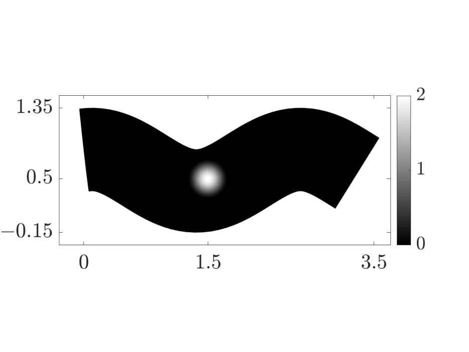
To mimic the laminar organization of cortical volumes [12, 3], we simulated a layered shape for this experiment. Figure 6(a) shows our simulated shape whose middle layer is the graph of x↦0.25​cos⁡(2.5​(x−0.1))+0.6x\mapsto 0.25\,\cos(2.5(x-0.1))+0.6. Other layers are generated through normal displacement starting from the middle layer with a step size 0.05. We use a parametric yank of the form of Example 4, that is,

(j(φ,θ)|v)=−∫φ⁡(M0)χgθ∘φ−1div(v)dx.(j(\varphi,\theta)\,|\,v)=-\int_{\varphi(M_{0})}\chi\ g_{\theta}\circ\varphi^{-1}\,\mathrm{div}(v)\,dx.

The potential gθg_{\theta} we used is a C1C^{1} compactly supported function

(12) g(c,h)​(x,r)={h​(|x−c|2r2−1)2 if ​|x−c|≤r0 otherwise .g_{(c,h)}(x;r)=\left\{\begin{array}[]{ll}\displaystyle h\left(\frac{|x-c|^{2}}{r^{2}}-1\right)^{2}&\mbox{ if }|x-c|\leq r\\ 0&\mbox{ otherwise }\end{array}\right..

Note that the parameter θ=(c,h)\theta=(c,h) is composed of the center c=(cx,cy)∈ℝ2c=(c_{x},c_{y})\in\mathbb{R}^{2} and the height h∈ℝh\in\mathbb{R}. We assume that the radius rr is known. Figure 6(b) shows the potential with c=(1.5,0.5)c=(1.5,0.5), h=2h=2, and r=0.25r=0.25. Given θ=(c,h)\theta=(c,h), we then computed the solution φθ\varphi_{\theta} to the system Eq. 4 under the layered elastic operator (equation Eq. 8) with λtan=0\lambda_{\mathrm{tan}}=0 and μtan=μtsv=μang=1\mu_{\mathrm{tan}}=\mu_{\mathrm{tsv}}=\mu_{\mathrm{ang}}=1. The deformation φθ​(1,M0)\varphi_{\theta}(1,M_{0}) is shown in Fig. 6(c), and the yank j​(φθ​(t),θ)j(\varphi_{\theta}(t),\theta) is shown in Fig. 6(d). The top and bottom layers of φθ​(1,M0)\varphi_{\theta}(1,M_{0}) were extracted as the target for our finite-dimensional optimization problem. Using a BFGS optimization method with multiple starting points sampled by a Latin hypercube design, we can retrieve (cx,cy,h)=(1.5,0.5,2)(c_{x},c_{y},h)=(1.5,0.5,2) within an absolute error 10−410^{-4}.

(a) Template.
Refer to caption
(b) Potential at time zero.
(c) Deformed template.
(d) Time-dependent yank induced by the transported potential.
Figure 6. Simulated data for the parametrized yank problem.

We now examine the robustness of our method when rr or the elastic parameters that are used in the inverse problem differ from those used to generate the target. In Fig. 7, we plot the computed minimizer θ∗=(cx∗,cy∗,h∗)\theta^{*}=(c_{x}^{*},c_{y}^{*},h^{*}) when we fix a different rr. While the retrieved height h∗h^{*} is inversely proportional to the radius rr with a fitted relationship h∗=𝒪⁡(r−2.37)h^{*}=\mathcal{O}(r^{-2.37}), the retrieved center (cx∗,cy∗)(c_{x}^{*},c_{y}^{*}) remains close to the true one (1.5,0.5)(1.5,0.5). We remark that the relationship h∗=𝒪⁡(r−p)h^{*}=\mathcal{O}(r^{-p}) was also observed in other simulated shapes, but with a different p>0p>0. The retrieved center is also quite stable when we vary the elastic parameters as we can see from Fig. 8, except for very small μtan\mu_{\mathrm{tan}} or μtsv\mu_{\mathrm{tsv}}.

Figure 7. Sensitivity of minimizers with respect to the radius of potential. Gray lines indicate the true parameters. The slope of the log-log plot on the right is −2.37-2.37.
Refer to caption
Refer to caption
Refer to caption
Figure 8. Sensitivity of minimizers with respect to elastic parameters.

5.2. 3D real data

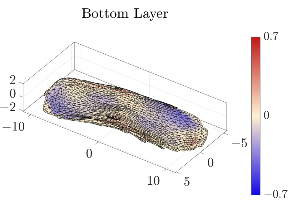
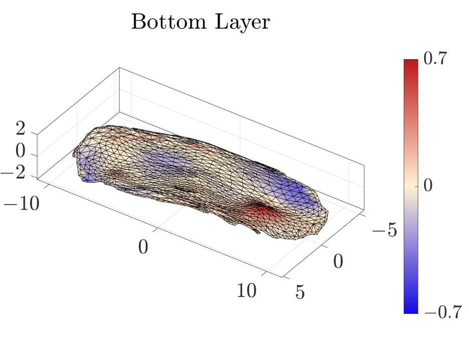
We now propose an experiment using 3D data derived from the BIOCARD dataset [25], which is a longitudinal study of Alzheimer’s disease. More precisely, the template and target shown in Fig. 9 were obtained by computing shape averages [23] of scans of the entorhinal cortex of subjects diagnosed with mild cognitive impairment in the cohort, using scans at the beginning of the study for the template, and after ten years of study for the target (the study is still ongoing with new scans being acquired). Participants enrolled in the BIOCARD cohort were all cognitively normal when the MRI scans were first acquired so that any observed atrophy in these brain volumes among those who progress to cognitive impairment provides significant information.

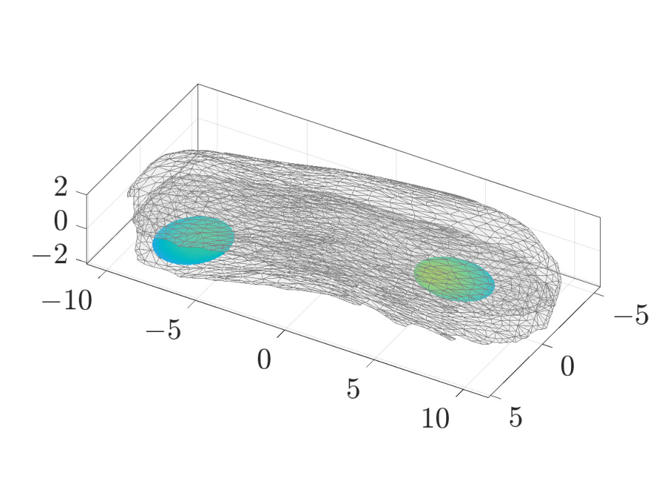
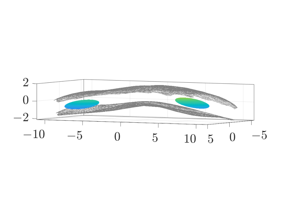
The layered structure on the source volume was inferred using the algorithm defined in [27, 36], which uses a normal propagation scheme between the lower and upper surfaces delimiting the shapes. The initial potential function estimated in this experiment is a sum of two compactly-supported functions such as defined in equation Eq. 12. Figure 10 summarizes the result that were obtained, with the location of the estimated potential and the resulting deformation. Note that these results are only provided here as an illustration of the proposed method, and we do not attempt to provide any new explanation yet on the pathogenesis of the disease. We hope, however, that this method may lead to new developments in this context in future work.

Refer to caption
(a) Template.
Refer to caption
(b) Target.
Refer to caption
Refer to caption
(c) Comparison between the template and target. The figures show the bottom and top layer of the template, and the color represents the zz-coordinate of the template minus the one of the target.
Figure 9. Entorhinal cortex volumes averaged over multiple patients from the BIOCARD dataset.
Refer to caption
Refer to caption
(a) Support of potential.
Refer to caption
Refer to caption
Refer to caption
Refer to caption
Refer to caption
Refer to caption
(b) Deformation. The color represents the Jacobian detD​φ​(t)\det D\varphi(t).
Refer to caption
Refer to caption
(c) Registration result. The figures show the bottom and top layer of the deformed template, and the color represents the zz-coordinate of the deformed template minus the one of the target.
Figure 10. Experimental results on averaged entorhinal cortex volumes.

6. Proofs

We now prove Theorems 1 and 2. The two proofs being similar, it will be convenient to address together parts (i) of both theorems, and then parts (ii) together.

6.1. Existence and uniqueness of solutions of controlled ODEs

We will use the following version of local existence and uniqueness for controlled ordinary differential equations. In the following, we will say that a function uu defined on [0,T][0,T] with values in a metric space UU is admissible if there exists a sequence of simple functions un:[0,T]→Uu_{n}:[0,T]\to U such that un​(t)u_{n}(t) converges to u⁡(t)u(t) for almost every t∈[0,T]t\in[0,T].

Theorem 3.

Let UU be a metric space, and let OO be an open subset of a Banach space 𝔹{\mathbb{B}}. Let F:U×O→𝔹F:U\times O\to{\mathbb{B}} be a continuous function that satisfies the following properties:

  1. (1)

    There exists a function γ:U→(0,∞)\gamma:U\to(0,\infty) such that, for all u∈Uu\in U, y∈Oy\in O:

    ‖F⁡(u,y)‖𝔹≤γ⁡(u)​(1+‖y‖𝔹).\|F(u,y)\|_{\mathbb{B}}\leq\gamma(u)\,(1+\|y\|_{\mathbb{B}})\,.
  2. (2)

    For all y0∈Oy_{0}\in O, there exists ry0>0r_{y_{0}}>0 and a function γy0:U→(0,+∞)\gamma_{y_{0}}:U\to(0,+\infty) such that for all y,y′∈Oy,y^{\prime}\in O with max⁡(‖y−y0‖𝔹,‖y′−y0‖𝔹)≤ry0\max(\|y-y_{0}\|_{\mathbb{B}},\|y^{\prime}-y_{0}\|_{\mathbb{B}})\leq r_{y_{0}} and all u∈Uu\in U

    (13) ‖F⁡(u,y)−F⁡(u,y′)‖𝔹≤γy0​(u)​‖y−y′‖𝔹.\|F(u,y)-F(u,y^{\prime})\|_{\mathbb{B}}\leq\gamma_{y_{0}}(u)\,\|y-y^{\prime}\|_{\mathbb{B}}\,.

Fix T>0T>0 and let u:[0,T]→Uu:[0,T]\to U be admissible such that (i) γ⁡(u⁡(t))\gamma(u(t)) is integrable on [0,T][0,T] and (ii) for all y0∈Oy_{0}\in O, γy0​(u​(t))\gamma_{y_{0}}(u(t)) is integrable on [0,T][0,T]. Then, for all y0∈Oy_{0}\in O, there exists a largest T0≤TT_{0}\leq T such that the ODE

∂ty⁡(t)=F⁡(u⁡(t),y⁡(t))\partial_{t}y(t)=F(u(t),y(t))

has a unique solution on [0,T0)[0,T_{0}) satisfying y⁡(0)=y0y(0)=y_{0}.
In addition, one has

(14) supt∈[0,T0)‖y⁡(t)‖𝔹≤C​exp⁡(∫0Tγ⁡(u⁡(s))​𝑑s).\sup_{t\,\in\,[0,T_{0})}\|y(t)\|_{\mathbb{B}}\leq C\exp\left(\int_{0}^{T}\gamma(u(s))ds\right).

where C=‖y0‖𝔹+∫0Tγ⁡(u⁡(s))​𝑑sC=\|y_{0}\|_{{\mathbb{B}}}+\int_{0}^{T}\gamma(u(s))ds is a constant that only depends on y0y_{0} and on the control uu. Moreover, y⁡(t)y(t) has a limit in 𝔹{\mathbb{B}} when tt tends to T0T_{0} and, if T0<TT_{0}<T, then limt→T0y⁡(t)∉O\lim_{t\to T_{0}}y(t)\not\in O.

Remark 5.

By a solution of ∂ty⁡(t)=F⁡(u⁡(t),y⁡(t))\partial_{t}y(t)=F(u(t),y(t)) over [0,T0)[0,T_{0}) we mean a continuous function y:[0.T0)→Oy:[0.T_{0})\to O satisfying

y⁡(t)=y0+∫0tF⁡(u⁡(s),y⁡(s))​𝑑sy(t)=y_{0}+\int_{0}^{t}F(u(s),y(s))ds

for all t∈[0,T0)t\in[0,T_{0}). The integral on the right-hand side is the Bochner integral. The fact that s↦F⁡(u⁡(s),y⁡(s))s\mapsto F(u(s),y(s)) is Bochner integrable is always true under the assumptions of Theorem 3, the proof being left to the reader.

Note that, letting y⁡(T0)=limt→T0y⁡(t)y(T_{0})=\lim_{t\to T_{0}}y(t), we have, taking limits on both sides,

y⁡(T0)=y0+∫0T0F⁡(u⁡(s),y⁡(s))​𝑑sy(T_{0})=y_{0}+\int_{0}^{T_{0}}F(u(s),y(s))ds
Proof.

The proof of the theorem is given here for completeness, and because the statement slightly deviates from that usually found in standard textbooks.

Fix y0∈Oy_{0}\in O and ry0,γy0r_{y_{0}},\gamma_{y_{0}} such that Eq. 13 is true. Let Ω\Omega denote the closed ball of center y0y_{0} and radius ry0r_{y_{0}} in 𝔹{\mathbb{B}}. Reducing ry0r_{y_{0}} if needed, assume that Ω⊂O\Omega\subset O. Introduce a small η>0\eta>0, let Iη=[0,η]I_{\eta}=[0,\eta] and let ℬη\mathcal{B}_{\eta} denote the complete metric space of continuous functions y:Iη→Ωy:I_{\eta}\to\Omega equipped with the metric d⁡(y,y′)=supt∈[0,η]‖y⁡(t)−y′​(t)‖𝔹d(y,y^{\prime})=\sup_{t\,\in\,[0,\eta]}\|y(t)-y^{\prime}(t)\|_{{\mathbb{B}}}. On this space, define, for t∈Iηt\in I_{\eta},

Γ⁡(y)​(t)=y0+∫0tF⁡(u⁡(s),y⁡(s))​𝑑s.\Gamma(y)(t)=y_{0}+\int_{0}^{t}F(u(s),y(s))ds.

Then, if y∈ℬηy\in\mathcal{B}_{\eta},

‖Γ⁡(y)​(t)−y0‖𝔹≤(1+‖y0‖𝔹+ry0)​∫0ηγ⁡(u⁡(s))​𝑑s\|\Gamma(y)(t)-y_{0}\|_{\mathbb{B}}\leq(1+\|y_{0}\|_{{\mathbb{B}}}+r_{y_{0}})\int_{0}^{\eta}\gamma(u(s))ds

so that Γ\Gamma maps ℬη\mathcal{B}_{\eta} onto itself as soon as ∫0ηγ0​(u⁡(s))​𝑑s≤ry0/(1+‖y0‖𝔹+ry0)\int_{0}^{\eta}\gamma_{0}(u(s))ds\leq r_{y_{0}}/(1+\|y_{0}\|_{{\mathbb{B}}}+r_{y_{0}}). Moreover, for all t∈Iηt\in I_{\eta} and all y,y′∈ℬηy,y^{\prime}\in\mathcal{B}_{\eta},

d⁡(Γ⁡(y)−Γ⁡(y′))≤(∫0ηγy0​(u⁡(s))​𝑑s)​d​(y,y′),d(\Gamma(y)-\Gamma(y^{\prime}))\leq\left(\int_{0}^{\eta}\gamma_{y_{0}}(u(s))ds\right)d(y,y^{\prime}),

which shows that Γ\Gamma is a contraction if ∫0ηγy0​(u⁡(s))​𝑑s<1\int_{0}^{\eta}\gamma_{y_{0}}(u(s))ds<1. Taking η\eta small enough, this shows that Γ\Gamma has a unique fixed point in ℬη\mathcal{B}_{\eta} and therefore proves local existence and uniqueness.

Now consider a solution yy defined on [0,T0)[0,T_{0}) with T0≤TT_{0}\leq T. For all 0≤t<T00\leq t<T_{0}:

‖y⁡(t)‖𝔹\displaystyle\|y(t)\|_{\mathbb{B}} ≤‖y0‖𝔹+∫0tγ⁡(u⁡(s))​(1+‖y⁡(s)‖𝔹)​𝑑s\displaystyle\leq\|y_{0}\|_{\mathbb{B}}+\int_{0}^{t}\gamma(u(s))(1+\|y(s)\|_{\mathbb{B}})ds
≤‖y0‖𝔹+∫0Tγ⁡(u⁡(s))​𝑑s+∫0tγ⁡(u⁡(s))​‖y⁡(s)‖𝔹​𝑑s,\displaystyle\leq\|y_{0}\|_{\mathbb{B}}+\int_{0}^{T}\gamma(u(s))ds+\int_{0}^{t}\gamma(u(s))\|y(s)\|_{\mathbb{B}}ds,

which by Gronwall’s inequality leads to

‖y⁡(t)‖𝔹≤(‖y0‖𝔹+∫0Tγ⁡(u⁡(s))​𝑑s)​exp⁡(∫0Tγ⁡(u⁡(s))​𝑑s)\|y(t)\|_{\mathbb{B}}\leq\left(\|y_{0}\|_{\mathbb{B}}+\int_{0}^{T}\gamma(u(s))ds\right)\exp\left(\int_{0}^{T}\gamma(u(s))ds\right)

and Eq. 14 follows by taking the supremum over all t∈[0,T0)t\in[0,T_{0}). Using this bound of solutions, we get that for all t,t′∈[0,T0)t,t^{\prime}\in[0,T_{0}):

‖y⁡(t′)−y⁡(t)‖𝔹≤∫tt′γ⁡(u⁡(s))​(1+‖y⁡(s)‖𝔹)​𝑑s≤C~​∫tt′γ⁡(u⁡(s))​𝑑s\|y(t^{\prime})-y(t)\|_{\mathbb{B}}\leq\int_{t}^{t^{\prime}}\gamma(u(s))(1+\|y(s)\|_{\mathbb{B}})ds\leq\widetilde{C}\int_{t}^{t^{\prime}}\gamma(u(s))ds

for some constant C~\widetilde{C} that depends on y0y_{0} and uu. This shows that yy can be extended by continuity to [0,T0][0,T_{0}]. Denote the limit by y⁡(T0)y(T_{0}): if T0<TT_{0}<T and y⁡(T0)∈Oy(T_{0})\in O, the solution can be extended further and we get a contradiction to the assumption that T0T_{0} defines the largest interval. This concludes the proof of Theorem 3. ∎

6.2. Proof of Theorem (i)

We now return to our original problem and first note, by stating the following lemma, that v⁡(t)v(t) in Eq. 1 is well defined.

Lemma 1.

If j∈V∗j\in V^{*} and φ∈𝐷𝑖𝑓𝑓𝑖𝑑1​(ℝ3)\varphi\in\mathit{Diff}_{\!\mathit{id}}^{1}(\mathbb{R}^{3}), then

f⁡(v)=ω2​‖v‖V2+12​(Aφ​v|v)−(j|v)f(v)=\frac{\omega}{2}\,\|v\|_{V}^{2}+\frac{1}{2}\,(A_{\varphi}\,v\,|\,v)-(j\,|\,v)

has a unique minimizer vφ,jv_{\varphi,\hskip 1.0ptj} in VV given by vφ,j=Lφ−1​jv_{\varphi,\hskip 1.0ptj}=L_{\varphi}^{-1}j, where Lφ=ω​KV−1+Aφ∈ℒ⁡(V,V∗)L_{\varphi}=\omega K_{V}^{-1}+A_{\varphi}\in\mathscr{L}(V,V^{*}).

Proof.

Since ff is strictly convex and differentiable with

D​f​(v)=(ω​KV−1+Aφ)​v−j=Lφ​v−j,Df(v)=(\omega K_{V}^{-1}+A_{\varphi})\,v-j=L_{\varphi}v-j,

the unique minimizer is characterized by D​f​(vφ,j)=0Df(v_{\varphi,\hskip 1.0ptj})=0, i.e., LφL_{\varphi} is invertible and vφ,j=Lφ−1​jv_{\varphi,\hskip 1.0ptj}=L_{\varphi}^{-1}j. ∎

System Eq. 1 can be rewritten as

∂tφ=F⁡(j,φ):=vφ,j∘φ\partial_{t}\varphi=F(j,\varphi):=v_{\varphi,j}\circ\varphi

and, letting φ=𝑖𝑑+h\varphi=\mathit{id}+h we want to apply Theorem 3 to the equation ∂th=F⁡(j,𝑖𝑑+h)\partial_{t}h=F(j,\mathit{id}+h), where we will take U=V∗U=V^{*}, 𝔹=C01​(ℝd,ℝd){\mathbb{B}}=C_{0}^{1}({\mathbb{R}}^{d},{\mathbb{R}}^{d}) and O=𝐷𝑖𝑓𝑓𝑖𝑑1​(ℝd)−𝑖𝑑O=\mathit{Diff}_{\!\mathit{id}}^{1}({\mathbb{R}}^{d})-\mathit{id}. We will show that the conditions for local existence are satisfied, and that, for any T0≤TT_{0}\leq T such that a solution exists over [0,T0)[0,T_{0}), the limit φ⁡(T0)\varphi(T_{0}) belongs to 𝐷𝑖𝑓𝑓𝑖𝑑1​(ℝd)\mathit{Diff}_{\!\mathit{id}}^{1}({\mathbb{R}}^{d}), which will prove existence on the full interval. Note that, by assumption, jj is Bochner integrable on [0,T][0,T] and therefore admissible in the sense of Theorem 3.

The following lemma summarizes some useful inequalities.

Lemma 2.
  1. (i)

    If v∈C01​(ℝ3,ℝ3)v\in C_{0}^{1}(\mathbb{R}^{3},\mathbb{R}^{3}) and φ∈𝐷𝑖𝑓𝑓𝑖𝑑1​(ℝ3)\varphi\in\mathit{Diff}_{\!\mathit{id}}^{1}({\mathbb{R}}^{3}), then v∘φ∈C01​(ℝ3,ℝ3)v\circ\varphi\in C_{0}^{1}(\mathbb{R}^{3},\mathbb{R}^{3}) and

    ‖v∘φ‖1,∞≤(2+‖φ−i​d‖1,∞)​‖v‖1,∞.\|v\circ\varphi\|_{1,\infty}\leq(2+\|\varphi-id\|_{1,\infty})\,\|v\|_{1,\infty}.
  2. (ii)

    If v∈C02​(ℝ3,ℝ3)v\in C_{0}^{2}(\mathbb{R}^{3},\mathbb{R}^{3}) and φ,ψ∈𝐷𝑖𝑓𝑓𝑖𝑑1​(ℝ3)\varphi,\psi\in\mathit{Diff}_{\!\mathit{id}}^{1}({\mathbb{R}}^{3}), then

    ‖v∘φ−v∘ψ‖1,∞≤(2+‖ψ−i​d‖1,∞)​‖v‖2,∞​‖φ−ψ‖1,∞.\|v\circ\varphi-v\circ\psi\|_{1,\infty}\leq(2+\|\psi-id\|_{1,\infty})\,\|v\|_{2,\infty}\,\|\varphi-\psi\|_{1,\infty}.
  3. (iii)

    If j∈V∗j\in V^{*} and φ∈𝐷𝑖𝑓𝑓𝑖𝑑1​(ℝ3)\varphi\in\mathit{Diff}_{\!\mathit{id}}^{1}(\mathbb{R}^{3}), then

    ‖vφ,j‖V=‖Lφ−1​j‖V≤1ω​‖j‖V∗,\|v_{\varphi,\hskip 1.0ptj}\|_{V}=\|L_{\varphi}^{-1}j\|_{V}\leq\frac{1}{\omega}\left\|j\right\|_{V^{*}},

    i.e., Lφ−1∈ℒ⁡(V∗,V)L_{\varphi}^{-1}\in\mathscr{L}(V^{*}\!,V) with ‖Lφ−1‖ℒ⁡(V∗,V)≤1ω\|L_{\varphi}^{-1}\|_{\mathscr{L}(V^{*}\!,\,V)}\leq\frac{1}{\omega}.

  4. (iv)

    If j∈V∗j\in V^{*} and φ,ψ∈𝐷𝑖𝑓𝑓𝑖𝑑1​(ℝ3)\varphi,\,\psi\in\mathit{Diff}_{\!\mathit{id}}^{1}(\mathbb{R}^{3}), then

    ‖Lφ−1−Lψ−1‖ℒ⁡(V∗,V)≤1ω2​‖Aφ−Aψ‖ℒ⁡(V,V∗),\|L_{\varphi}^{-1}-L_{\psi}^{-1}\|_{\mathscr{L}(V^{*}\!,\,V)}\leq\frac{1}{\omega^{2}}\,\|A_{\varphi}-A_{\psi}\|_{\mathscr{L}(V,\,V^{*})},

    which implies

    ‖vφ,j−vψ,j‖V≤1ω2​‖Aφ−Aψ‖ℒ⁡(V,V∗)​‖j‖V∗.\|v_{\varphi,\hskip 1.0ptj}-v_{\psi,\hskip 1.0ptj}\|_{V}\leq\frac{1}{\omega^{2}}\,\|A_{\varphi}-A_{\psi}\|_{\mathscr{L}(V,\,V^{*})}\,\|j\|_{V^{*}}.
Proof.

The proofs of (i) and (ii) are straightforward applications of the chain rule and left to the reader. To show (iii), it is equivalent to prove that, for all v∈Vv\in V, ‖v‖V≤(1/ω)​‖Lφ​v‖V∗\|v\|_{V}\leq(1/\omega)\left\|L_{\varphi}\,v\right\|_{V^{*}} . We have, letting 𝐼𝑑V\mathit{Id}_{V} denote the identity operator on VV,

(1ω​‖Lφ​v‖V∗)2\displaystyle\left(\frac{1}{\omega}\left\|L_{\varphi}\,v\right\|_{V^{*}}\right)^{2} =(1ω​‖KV​(ω​KV−1+Aφ)​v‖V)2\displaystyle=\left(\frac{1}{\omega}\left\|K_{V}\left(\omega K_{V}^{-1}+A_{\varphi}\right)v\right\|_{V}\right)^{2}
=1ω2​‖(ω​𝐼𝑑V+KV​Aφ)​v‖V2\displaystyle=\frac{1}{\omega^{2}}\left\|\left(\omega\,\mathit{Id}_{V}+K_{V}A_{\varphi}\right)v\right\|_{V}^{2}
=‖v‖V2+1ω2​‖KV​Aφ​v‖V2+2ω​⟨v,KV​Aφ​v⟩V\displaystyle=\|v\|_{V}^{2}+\frac{1}{\omega^{2}}\,\|K_{V}A_{\varphi}\hskip 1.0ptv\|_{V}^{2}+\frac{2}{\omega}\,\langle v,K_{V}A_{\varphi}\hskip 1.0ptv\rangle_{V}
=‖v‖V2+1ω2​‖KV​Aφ​v‖V2+2ω​(Aφ​v|v)≥‖v‖V2,\displaystyle=\|v\|_{V}^{2}+\frac{1}{\omega^{2}}\,\|K_{V}A_{\varphi}\hskip 1.0ptv\|_{V}^{2}+\frac{2}{\omega}\,(A_{\varphi}\hskip 1.0ptv\,|\,v)\,\geq\,\|v\|_{V}^{2},

where the last inequality follows from (Aφ​v|v)≥0(A_{\varphi}\hskip 1.0ptv\,|\,v)\geq 0.

We now prove (iv), writing:

‖Lφ−1−Lψ−1‖ℒ⁡(V∗,V)\displaystyle\|L_{\varphi}^{-1}-L_{\psi}^{-1}\|_{\mathscr{L}(V^{*}\!,\,V)} =‖Lφ−1​(Lψ−Lφ)​Lψ−1‖ℒ⁡(V∗,V)\displaystyle=\left\|L_{\varphi}^{-1}\left(L_{\psi}-L_{\varphi}\right)L_{\psi}^{-1}\right\|_{\mathscr{L}(V^{*}\!,\,V)}
=‖Lφ−1​(Aψ−Aφ)​Lψ−1‖ℒ⁡(V∗,V)\displaystyle=\left\|L_{\varphi}^{-1}\left(A_{\psi}-A_{\varphi}\right)L_{\psi}^{-1}\right\|_{\mathscr{L}(V^{*}\!,\,V)}
≤‖Lφ−1‖ℒ⁡(V∗,V)​‖Aφ−Aψ‖ℒ⁡(V,V∗)​‖Lψ−1‖ℒ⁡(V∗,V)\displaystyle\leq\|L_{\varphi}^{-1}\|_{\mathscr{L}(V^{*}\!,\,V)}\ \|A_{\varphi}-A_{\psi}\|_{\mathscr{L}(V,\,V^{*})}\ \|L_{\psi}^{-1}\|_{\mathscr{L}(V^{*}\!,\,V)}\
≤1ω2​‖Aφ−Aψ‖ℒ⁡(V,V∗),\displaystyle\leq\frac{1}{\omega^{2}}\,\|A_{\varphi}-A_{\psi}\|_{\mathscr{L}(V,\,V^{*})},

since (iii) implies that ‖Lφ−1‖ℒ⁡(V∗,V)≤(1/ω)\|L_{\varphi}^{-1}\|_{\mathscr{L}(V^{*}\!,\,V)}\leq({1}/{\omega}). ∎

Corollary 1.

Let F⁡(j,φ)=vφ,j∘φF(j,\varphi)=v_{\varphi,j}\circ\varphi be defined on V∗×𝐷𝑖𝑓𝑓𝑖𝑑1​(ℝd)V^{*}\times\mathit{Diff}_{\!\mathit{id}}^{1}({\mathbb{R}}^{d}). Then, FF is continuous and for all j∈V∗j\in V^{*}, and φ∈𝐷𝑖𝑓𝑓𝑖𝑑1​(ℝd)\varphi\in\mathit{Diff}_{\!\mathit{id}}^{1}({\mathbb{R}}^{d}),

‖F⁡(j,φ)‖1,∞≤2​cVω​(1+‖φ−𝑖𝑑‖1,∞)​‖j‖V∗\|F(j,\varphi)\|_{1,\infty}\leq\frac{2c_{V}}{\omega}(1+\|\varphi-\mathit{id}\|_{1,\infty})\|j\|_{V^{*}}

so that the assumption Theorem (1) holds for F~:(j,h)↦F⁡(j,𝑖𝑑+h)\tilde{F}:(j,h)\mapsto F(j,\mathit{id}+h) with γ⁡(j)=(2​cV/ω)​‖j‖V∗\gamma(j)=(2c_{V}/\omega)\|j\|_{V^{*}}.

Moreover, for all j∈V∗j\in V^{*}, and φ,ψ∈𝐷𝑖𝑓𝑓𝑖𝑑1​(ℝd)\varphi,\psi\in\mathit{Diff}_{\!\mathit{id}}^{1}({\mathbb{R}}^{d})

‖F⁡(j,φ)−F⁡(j,ψ)‖1,∞≤Cψ​(‖φ−ψ‖1,∞+‖Aφ−Aψ‖ℒ⁡(V,V∗))​‖j‖V∗.\|F(j,\varphi)-F(j,\psi)\|_{1,\infty}\leq C_{\psi}\,(\|\varphi-\psi\|_{1,\infty}+\|A_{\varphi}-A_{\psi}\|_{\mathscr{L}(V,\,V^{*})})\|j\|_{V^{*}}.

Thus, if AφA_{\varphi} is locally Lipschitz, so is FF and F~\tilde{F}, and the assumption Theorem (2) holds.

Proof.

We have

‖F⁡(j,φ)‖1,∞\displaystyle\|F(j,\varphi)\|_{1,\infty} ≤(2+‖φ−𝑖𝑑‖1,∞)​‖vφ,j‖1,∞\displaystyle\leq(2+\|\varphi-\mathit{id}\|_{1,\infty})\|v_{\varphi,j}\|_{1,\infty}
≤cV​(2+‖φ−𝑖𝑑‖1,∞)​‖vφ,j‖V\displaystyle\leq c_{V}(2+\|\varphi-\mathit{id}\|_{1,\infty})\|v_{\varphi,j}\|_{V}
≤cVω​(2+‖φ−𝑖𝑑‖1,∞)​‖j‖V∗.\displaystyle\leq\frac{c_{V}}{\omega}(2+\|\varphi-\mathit{id}\|_{1,\infty})\|j\|_{V^{*}}\,.

This inequality also shows the continuity of FF in jj, since F⁡(j,φ)=(Lφ−1​j)∘φF(j,\varphi)=(L_{\varphi}^{-1}j)\circ\varphi is linear in jj.

Similarly

‖F⁡(j,φ)−F⁡(j,ψ)‖1,∞\displaystyle\|F(j,\varphi)-F(j,\psi)\|_{1,\infty} ≤‖vφ,j∘φ−vφ,j∘ψ‖1,∞+‖vφ,j∘ψ−vψ,j∘ψ‖1,∞\displaystyle\leq\|v_{\varphi,j}\circ\varphi-v_{\varphi,j}\circ\psi\|_{1,\infty}+\|v_{\varphi,j}\circ\psi-v_{\psi,j}\circ\psi\|_{1,\infty}
≤(2+‖ψ−𝑖𝑑‖1,∞)​‖φ−ψ‖1,∞​‖vφ,j‖2,∞\displaystyle\leq(2+\|\psi-\mathit{id}\|_{1,\infty})\|\varphi-\psi\|_{1,\infty}\|v_{\varphi,j}\|_{2,\infty}
+(2+‖ψ−𝑖𝑑‖1,∞)​‖vφ,j−vψ,j‖1,∞\displaystyle+(2+\|\psi-\mathit{id}\|_{1,\infty})\|v_{\varphi,j}-v_{\psi,j}\|_{1,\infty}
≤cVω​(2+‖ψ−𝑖𝑑‖1,∞)​‖φ−ψ‖1,∞​‖j‖V∗\displaystyle\leq\frac{c_{V}}{\omega}(2+\|\psi-\mathit{id}\|_{1,\infty})\|\varphi-\psi\|_{1,\infty}\|j\|_{V^{*}}
+1ω2​(2+‖ψ−𝑖𝑑‖1,∞)​‖Aφ−Aψ‖ℒ⁡(V,V∗)​‖j‖V∗.\displaystyle+\frac{1}{\omega^{2}}(2+\|\psi-\mathit{id}\|_{1,\infty})\,\|A_{\varphi}-A_{\psi}\|_{\mathscr{L}(V,\,V^{*})}\|j\|_{V^{*}}.

Since F⁡(j,φ)F(j,\varphi) is continuous and linear in jj and continuous in φ\varphi, we know that FF is continuous. ∎

Corollary 1 therefore implies that Eq. 1 has a unique local solution as soon as j⁡(t)j(t) is integrable. To conclude the proof of (i) in Theorem 1, it suffices to show that any solution on an interval [0,T0)[0,T_{0}) is such that φ(T0):⁣=limt↑T0φ(t)∈𝐷𝑖𝑓𝑓𝑖𝑑1(ℝd)\varphi(T_{0})\mathrel{\mathchoice{\vbox{\hbox{$\displaystyle:$}}}{\vbox{\hbox{$\textstyle:$}}}{\vbox{\hbox{$\scriptstyle:$}}}{\vbox{\hbox{$\scriptscriptstyle:$}}}{=}}\lim_{t\,\uparrow\,T_{0}}\varphi(t)\in\mathit{Diff}_{\!\mathit{id}}^{1}({\mathbb{R}}^{d}). This is true because, if one lets w⁡(t)=vφ⁡(t),j⁡(t)w(t)=v_{\varphi(t),j(t)}, then w∈L1​([0,T0],V)w\in L^{1}([0,T_{0}],V) and φ\varphi is, by construction, the flow associated to the ordinary differential equation ∂tz=w⁡(t,z)\partial_{t}z=w(t,z), i.e., it satisfies ∂tφ⁡(t,x)=w⁡(t,φ⁡(t,x))\partial_{t}\varphi(t,x)=w(t,\varphi(t,x)). This shows that (see, e.g., [33] Chap. 8) φ∈C⁡([0,T0],𝐷𝑖𝑓𝑓𝑖𝑑2​(ℝ3))\varphi\in C([0,T_{0}],\mathit{Diff}_{\!\mathit{id}}^{2}(\mathbb{R}^{3})), which completes the proof of part (i) of Theorem 1.

In particular, for t∈[0,T0]t\in[0,T_{0}], one has φ​(t,⋅)−1=ψ⁡(t,⋅)\varphi(t,\cdot)^{-1}=\psi(t,\cdot) where ψ\psi is the flow associated with the equation ∂sz=w~(t)​(s,z)\partial_{s}z=\tilde{w}^{(t)}(s,z), with w~(t)​(s)=−vφ⁡(t−s),j⁡(t−s)\tilde{w}^{(t)}(s)=-v_{\varphi(t-s),j(t-s)}. Note that we have not defined ww at time T0T_{0} (or w~\tilde{w} at time 0), which is not a problem since these time-dependent vector fields only need to be defined almost everywhere (in tt) for the result to hold. (One can actually show using Cauchy sequences that w⁡(t)w(t) has a limit when tt tends to T0T_{0} anyway).

We also point out that, using the inequalities of Lemma 2, the transcription of Eq. 14 to the present case becomes ‖φ⁡(t)−i​d‖1,∞≤Bj\|\varphi(t)-id\|_{1,\infty}\leq B_{j} with

(15) Bj=2​cvω​‖j‖𝒳V∗,T1​exp⁡(cVω​‖j‖𝒳V∗,T1).B_{j}=\frac{2c_{v}}{\omega}\|j\|_{\mathcal{X}^{1}_{V^{*}\!,\,T}}\exp\!\left(\frac{c_{V}}{\omega}\,\|j\|_{\mathcal{X}_{V^{*}\!,\,T}^{1}}\right).

(here, the initial condition is always φ⁡(0,⋅)=𝑖𝑑\varphi(0,\cdot)=\mathit{id}) and thus BjB_{j} only depends on jj.

We also have ‖φ−1​(t)−i​d‖1,∞≤Bj\|\varphi^{-1}(t)-id\|_{1,\infty}\leq B_{j}. This can be proved for each tt by applying Theorem 3 to F⁡(w~,ψ)=w~∘ψF(\tilde{w},\psi)=\tilde{w}\circ\psi, with U=VU=V, which satisfies the hypotheses with γ⁡(w~)=cV​‖w~‖V\gamma(\tilde{w})=c_{V}\|\tilde{w}\|_{V}. To obtain the same constant BjB_{j}, one only needs to notice that, for all ss, ‖w~(t)​(s)‖V=‖w⁡(t−s)‖V\|\tilde{w}^{(t)}(s)\|_{V}=\|w(t-s)\|_{V}

We summarize this discussion in the next lemma.

Lemma 3.

Suppose that j∈𝒳V∗,T1j\in\mathcal{X}_{V^{*}\!,\,T}^{1}. If φ∈C⁡([0,T0],𝐷𝑖𝑓𝑓𝑖𝑑1​(ℝ3))\varphi\in C([0,T_{0}],\mathit{Diff}_{\!\mathit{id}}^{1}(\mathbb{R}^{3})) is a local solution to system Eq. 1 for some T0≤TT_{0}\leq T, then ‖φ⁡(t)−i​d‖1,∞≤Bj\|\varphi(t)-id\|_{1,\infty}\leq B_{j} and ‖φ−1​(t)−i​d‖1,∞≤Bj\|\varphi^{-1}(t)-id\|_{1,\infty}\leq B_{j} for all t∈[0,T0]t\in[0,T_{0}], where BjB_{j} is defined in equation Eq. 15.

Moreover, the local solution φ\varphi is actually in C⁡([0,T0],𝐷𝑖𝑓𝑓𝑖𝑑2​(ℝ3))C([0,T_{0}],\mathit{Diff}_{\!\mathit{id}}^{2}(\mathbb{R}^{3})) and there exists a constant CjC_{j} such that

(16) ‖D2​φ​(t)‖∞≤Cj​exp⁡(cVω​‖j‖𝒳V∗,T1)\|D^{2}\varphi(t)\|_{\infty}\leq C_{j}\exp\!\left(\frac{c_{V}}{\omega}\,\|j\|_{\mathcal{X}_{V^{*}\!,\,T}^{1}}\right)

for all t∈[0,T0]t\in[0,T_{0}].

Only the last inequality remains to be shown. We have

(17) |D2​φ​(t,x)|≤∫0t(|D2​vφ⁡(s),j⁡(s)​(φ⁡(s,x))|​|D​φ​(s,x)|2CLOSEOPEN+|D​vφ⁡(s),j⁡(s)​(φ⁡(s,x))|​|D2​φ​(s,x)|)​d​s,≤cVω​‖j‖χV∗,T1​‖D​φ​(t)‖∞2+cVω​∫0t‖j⁡(s)‖V∗​|D2​φ​(s,x)|​𝑑s\displaystyle\begin{split}|D^{2}\varphi(t,x)|&\leq\int_{0}^{t}\left(\vphantom{\sum}|D^{2}v_{\varphi(s),\hskip 1.0ptj(s)}(\varphi(s,x))|\,|D\varphi(s,x)|^{2}\right.\\ &\hskip 30.0pt\left.\vphantom{\sum}\phantom{}+|Dv_{\varphi(s),\hskip 1.0ptj(s)}(\varphi(s,x))|\,|D^{2}\varphi(s,x)|\right)ds,\\ &\leq\frac{c_{V}}{\omega}\|j\|_{\chi^{1}_{V^{*}\!,\,T}}\|D\varphi(t)\|^{2}_{\infty}+\frac{c_{V}}{\omega}\int_{0}^{t}\|j(s)\|_{V^{*}}|D^{2}\varphi(s,x)|\,ds\end{split}

and inequality Eq. 16 follows from Gronwall’s lemma, since ‖D​φ​(t)‖∞2≤(1+Bj)2\|D\varphi(t)\|^{2}_{\infty}\leq(1+B_{j})^{2}.

6.3. Proof of Theorem (i)

Denote vφ,θ=vφ,j⁡(φ,θ)v_{\varphi,\theta}=v_{\varphi,j(\varphi,\theta)} and let

Gθ​(φ)=vφ,θ∘φ.G_{\theta}(\varphi)=v_{\varphi,\theta}\circ\varphi.

We only need to apply the standard existence theorem for the ODE ∂tφ=Gθ​(φ)\partial_{t}\varphi=G_{\theta}(\varphi). For this, it is sufficient to prove that, for any θ∈Θ\theta\in\Theta,

  1. (1)

    There exists γ>0\gamma>0 such that, for all φ∈𝐷𝑖𝑓𝑓𝑖𝑑1​(ℝd)\varphi\in\mathit{Diff}_{\!\mathit{id}}^{1}({\mathbb{R}}^{d}):

    ‖Gθ​(φ)‖1,∞≤γ⁡(1+‖φ−𝑖𝑑‖1,∞).\|G_{\theta}(\varphi)\|_{1,\infty}\leq\gamma(1+\|\varphi-\mathit{id}\|_{1,\infty})\,.
  2. (2)

    For all φ0∈𝐷𝑖𝑓𝑓𝑖𝑑1​(ℝd)\varphi_{0}\in\mathit{Diff}_{\!\mathit{id}}^{1}({\mathbb{R}}^{d}), there exists rφ0>0r_{\varphi_{0}}>0 and γφ0>0\gamma_{\varphi_{0}}>0 such that for all φ,ψ∈𝐷𝑖𝑓𝑓𝑖𝑑1​(ℝd)\varphi,\psi\in\mathit{Diff}_{\!\mathit{id}}^{1}({\mathbb{R}}^{d}) with max⁡(‖φ−φ0‖𝔹,‖ψ−φ0‖𝔹)≤rφ0\max(\|\varphi-\varphi_{0}\|_{\mathbb{B}},\|\psi-\varphi_{0}\|_{\mathbb{B}})\leq r_{\varphi_{0}}

    ‖Gθ​(φ)−Gθ​(ψ)‖1,∞≤γφ0​‖φ−ψ‖1,∞.\|G_{\theta}(\varphi)-G_{\theta}(\psi)\|_{1,\infty}\leq\gamma_{\varphi_{0}}\|\varphi-\psi\|_{1,\infty}\,.

These properties are easily deduced from Lemma 2 and the boundedness and Lipschitz assumptions made on j⁡(φ,θ)j(\varphi,\theta), and we skip the argument.

6.4. Proof of Theorem (ii)

Given j∈𝒳V∗,T2⊂𝒳V∗,T1j\in\mathcal{X}_{V^{*}\!,\,T}^{2}\subset\mathcal{X}_{V^{*}\!,\,T}^{1}, we have proved that system Eq. 1 has a unique solution φj∈C⁡([0,T],𝐷𝑖𝑓𝑓𝑖𝑑2​(ℝ3))\varphi_{j}\in C([0,T],\mathit{Diff}_{\!\mathit{id}}^{2}(\mathbb{R}^{3})). Denote the well-defined objective function by

f⁡(j)=∫0T(j⁡(t)|vφj​(t),j​(t))​𝑑t+ρ⁡(φj​(T,M0),Mtarg).f(j)=\int_{0}^{T}(j(t)\,|\,v_{\varphi_{j}(t),\hskip 1.0ptj(t)})\,dt+\rho(\varphi_{j}(T,M_{0}),M_{\mathrm{targ}}).

To prove the existence of minimizers of ff, we show that minimizing sequences of ff are bounded and ff is weakly sequentially lower semicontinuous. Since 𝒳V∗,T2\mathcal{X}_{V^{*}\!,\,T}^{2} is a Hilbert space, the existence of minimizers will follow by applying the direct method of the calculus of variations.

Lemma 4.

Minimizing sequences of ff are bounded.

Proof.

Let (jn)n=1∞(j_{n})_{n=1}^{\infty} be a minimizing sequence of ff. We denote for short vn(t):⁣=vφjn​(t),jn​(t)v_{n}(t)\mathrel{\mathchoice{\vbox{\hbox{$\displaystyle:$}}}{\vbox{\hbox{$\textstyle:$}}}{\vbox{\hbox{$\scriptstyle:$}}}{\vbox{\hbox{$\scriptscriptstyle:$}}}{=}}v_{\varphi_{j_{n}}\!(t),\hskip 1.0ptj_{n}(t)}. Note that the solution of j≡0j\equiv 0 is φj≡𝑖𝑑\varphi_{j}\equiv\mathit{id}, so we can assume f⁡(jn)≤f⁡(0)=ρ⁡(M0,Mtarg)f(j_{n})\leq f(0)=\rho(M_{0},M_{\mathrm{targ}}) without loss of generality. Using Lemma 1, we have jn​(t)=(ω​KV−1+Aφjn​(t))​vn​(t)j_{n}(t)=(\omega K_{V}^{-1}+A_{\varphi_{j_{n}}\!(t)})\,v_{n}(t). It follows that

(18) ρ⁡(M0,Mtarg)≥f⁡(jn)≥∫0T(jn​(t)|vn​(t))​𝑑t≥∫0Tω⁡(KV−1​vn​(t)|vn​(t))​𝑑t=ω​∫0T‖vn​(t)‖V2​dt≥ωT​(∫0T‖vn​(t)‖V​dt)2\displaystyle\begin{split}\rho(M_{0},M_{\mathrm{targ}})&\geq f(j_{n})\geq\int_{0}^{T}(j_{n}(t)\,|\,v_{n}(t))\,dt\\ &\geq\int_{0}^{T}\omega\,(K_{V}^{-1}v_{n}(t)\,|\,v_{n}(t))\,dt\\ &=\omega\int_{0}^{T}\|v_{n}(t)\|_{V}^{2}\,dt\geq\frac{\omega}{T}\left(\int_{0}^{T}\|v_{n}(t)\|_{V}\,dt\right)^{2}\end{split}

From Theorem 3 (applied to F⁡(v,h)=v∘(𝑖𝑑+h)F(v,h)=v\circ(\mathit{id}+h) and U=VU=V), we know that the boundedness of ∫0T‖vn​(t)‖V​𝑑t\int_{0}^{T}\|v_{n}(t)\|_{V}\,dt implies the boundedness of solutions, i.e., there exists a constant BB such that ‖φjn​(t)−𝑖𝑑‖1,∞≤B\|\varphi_{j_{n}}\!(t)-\mathit{id}\|_{1,\infty}\leq B for all t∈[0,T]t\in[0,T] and n∈ℕn\in\mathbb{N}. Since φ↦Aφ\varphi\mapsto A_{\varphi} is Lipschitz with respect to the seminorm ∥⋅∥1,∞M0\|\cdot\|_{1,\infty}^{M_{0}} on 𝔖B\mathfrak{S}_{B}, denoting the Lipschitz constant by ℓA​(B)\ell_{A}(B) leads to

‖Aφjn​(t)‖ℒ⁡(V,V∗)≤‖A𝑖𝑑‖ℒ⁡(V,V∗)+ℓA​‖φjn​(t)−𝑖𝑑‖1,∞M0≤CB.\|A_{\varphi_{j_{n}}\!(t)}\|_{\mathscr{L}(V,\,V^{*})}\leq\|A_{\mathit{id}}\|_{\mathscr{L}(V,\,V^{*})}+\ell_{A}\,\|\varphi_{j_{n}}\!(t)-\mathit{id}\|_{1,\infty}^{M_{0}}\leq C_{B}.

Now we return to inequality Eq. 18 and write

ρ⁡(M0,Mtarg)\displaystyle\rho(M_{0},M_{\mathrm{targ}}) ≥ω​∫0T‖vn​(t)‖V2​𝑑t\displaystyle\geq\omega\int_{0}^{T}\|v_{n}(t)\|_{V}^{2}\,dt
≥ω​∫0T(‖jn​(t)‖V∗‖ω​KV−1+Aφjn​(t)‖ℒ⁡(V,V∗))2​𝑑t\displaystyle\geq\omega\int_{0}^{T}\left(\frac{\|j_{n}(t)\|_{V^{*}}}{\|\omega K_{V}^{-1}+A_{\varphi_{j_{n}}\!(t)}\|_{\mathscr{L}(V,\,V^{*})}}\right)^{2}dt
≥ω​∫0T(‖jn​(t)‖V∗ω+CB)2​𝑑t=CB​‖jn‖𝒳V∗,T22,\displaystyle\geq\omega\int_{0}^{T}\left(\frac{\|j_{n}(t)\|_{V^{*}}}{\omega+C_{B}}\right)^{2}dt=C_{B}\,\|j_{n}\|_{\mathcal{X}_{V^{*}\!,\,T}^{2}}^{2},

where we have used the fact that KV−1K_{V}^{-1} is an isometry from VV to V∗V^{*} in the third inequality. The above inequality shows that a minimizing sequence (jn)n=1∞(j_{n})_{n=1}^{\infty} is bounded. ∎

To prove that ff is weakly sequentially lower semicontinuous, we separate the two terms in ff and show in Lemmas 6 and 7 respectively that the first term j↦∫0T(j⁡(t)|vφj​(t),j​(t))​𝑑tj\mapsto\int_{0}^{T}(j(t)\,|\,v_{\varphi_{j}(t),j(t)})\,dt and the second term j↦ρ⁡(φj​(T,M0),Mtarg)j\mapsto\rho(\varphi_{j}(T,M_{0}),M_{\mathrm{targ}}) are both weakly sequentially lower semicontinuous.

Let jn⇀jj_{n}\rightharpoonup j in 𝒳V∗,T2\mathcal{X}_{V^{*}\!,\,T}^{2}. We first derive some preliminary bounds that will be used in the following Lemmas 5, 6, and 7. Since jn⇀jj_{n}\rightharpoonup j, there exists J>0J>0 such that ‖jn‖𝒳V∗,T2≤J\|j_{n}\|_{\mathcal{X}_{V^{*}\!,\,T}^{2}}\leq J for all n∈ℕn\in\mathbb{N}. It follows that

‖j‖𝒳V∗,T2≤lim infn→∞‖jn‖𝒳V∗,T2≤J.\|j\|_{\mathcal{X}_{V^{*}\!,\,T}^{2}}\leq\liminf_{n\rightarrow\infty}\|j_{n}\|_{\mathcal{X}_{V^{*}\!,\,T}^{2}}\leq J.

For the solution φjn\varphi_{j_{n}}, Lemma 3 shows that for every t∈[0,T]t\in[0,T]

‖φjn​(t)−𝑖𝑑‖1,∞≤2​cVω​‖jn‖𝒳V∗,T1​exp⁡(cVω​‖jn‖𝒳V∗,T1),\|\varphi_{j_{n}}\!(t)-\mathit{id}\|_{1,\infty}\leq\frac{2c_{V}}{\omega}\,\|j_{n}\|_{\mathcal{X}_{V^{*}\!,\,T}^{1}}\exp\!\left({\frac{c_{V}}{\omega}\|j_{n}\|_{\mathcal{X}_{V^{*}\!,\,T}^{1}}}\right),

so

‖φjn​(t)−𝑖𝑑‖1,∞≤2​cVω​J​T​exp⁡(cVω​J​T)=:BJ.\|\varphi_{j_{n}}\!(t)-\mathit{id}\|_{1,\infty}\leq\frac{2c_{V}}{\omega}\,J\sqrt{T}\ \exp\!\left({\frac{c_{V}}{\omega}J\sqrt{T}}\right)\mathrel{{=}\mathchoice{\vbox{\hbox{$\displaystyle:$}}}{\vbox{\hbox{$\textstyle:$}}}{\vbox{\hbox{$\scriptstyle:$}}}{\vbox{\hbox{$\scriptscriptstyle:$}}}}B_{J}.

Similarly, we have

‖φj​(t)−𝑖𝑑‖1,∞\displaystyle\|\varphi_{j}(t)-\mathit{id}\|_{1,\infty} ≤2​cVω​‖j‖𝒳V∗,T1​exp⁡(cVω​‖j‖𝒳V∗,T1)\displaystyle\leq\frac{2c_{V}}{\omega}\,\|j\|_{\mathcal{X}_{V^{*}\!,\,T}^{1}}\exp\!\left({\frac{c_{V}}{\omega}\|j\|_{\mathcal{X}_{V^{*}\!,\,T}^{1}}}\right)
≤2​cVω​J​T​exp⁡(cVω​J​T)=BJ.\displaystyle\leq\frac{2c_{V}}{\omega}\,J\sqrt{T}\ \exp\!\left({\frac{c_{V}}{\omega}J\sqrt{T}}\right)=B_{J}.

Still from Lemma 3, it also holds that

‖φjn−1​(t)−𝑖𝑑‖1,∞≤BJ and ‖φj−1​(t)−𝑖𝑑‖1,∞≤BJ.\|\varphi_{j_{n}}^{-1}(t)-\mathit{id}\|_{1,\infty}\leq B_{J}\ \ \mbox{ and }\ \ \|\varphi_{j}^{-1}(t)-\mathit{id}\|_{1,\infty}\leq B_{J}.

We then have (φjn)n=1∞⊂𝔖BJ(\varphi_{j_{n}})_{n=1}^{\infty}\subset\mathfrak{S}_{B_{J}} and φj∈𝔖BJ\varphi_{j}\in\mathfrak{S}_{B_{J}}, where 𝔖BJ\mathfrak{S}_{B_{J}} is defined in the statement of the theorem.

The following lemma is a preliminary step towards Lemmas 6 and 7, which prove the weakly sequentially lower semicontinuity of ff.

Lemma 5.

If jn⇀jj_{n}\rightharpoonup j in 𝒳V∗,T2\mathcal{X}_{V^{*}\!,\,T}^{2}, then ‖φjn​(t)−φj​(t)‖1,∞M0→0\|\varphi_{j_{n}}\!(t)-\varphi_{j}(t)\|_{1,\infty}^{M_{0}}\rightarrow 0 for all t∈[0,T]t\in[0,T].

Proof.

Note that

φjn​(t,x)−φj​(t,x)\displaystyle\hskip 14.0pt\varphi_{j_{n}}\!(t,x)-\varphi_{j}(t,x)
=∫0t(vφjn​(s),jn​(s)​(φjn​(s,x))−vφj​(s),j​(s)​(φj​(s,x)))​𝑑s\displaystyle=\int_{0}^{t}\left(v_{\varphi_{j_{n}}\!(s),\hskip 1.0ptj_{n}(s)}(\varphi_{j_{n}}\!(s,x))-v_{\varphi_{j}(s),\hskip 1.0ptj(s)}(\varphi_{j}(s,x))\right)ds
=∫0t((Lφjn​(s)−1​jn​(s))​(φjn​(s,x))−(Lφj​(s)−1​jn​(s))​(φjn​(s,x)))​𝑑s\displaystyle=\int_{0}^{t}\left(\left(L_{\varphi_{j_{n}}\!(s)}^{-1}\,j_{n}(s)\right)(\varphi_{j_{n}}\!(s,x))-\left(L_{\varphi_{j}(s)}^{-1}\,j_{n}(s)\right)(\varphi_{j_{n}}\!(s,x))\right)ds
+∫0t((Lφj​(s)−1jn(s))(φjn(s,x))−(Lφj​(s)−1jn(s))(φj(s,x)))ds\displaystyle\hskip 12.0pt\phantom{}+\int_{0}^{t}\left(\left(L_{\varphi_{j}(s)}^{-1}\,j_{n}(s)\right)(\varphi_{j_{n}}\!(s,x))-\left(L_{\varphi_{j}(s)}^{-1}\,j_{n}(s)\right)(\varphi_{j}(s,x))\right)ds
+∫0t((Lφj​(s)−1jn(s))(φj(s,x))−(Lφj​(s)−1j(s))(φj(s,x)))ds\displaystyle\hskip 12.0pt\phantom{}+\int_{0}^{t}\left(\left(L_{\varphi_{j}(s)}^{-1}\,j_{n}(s)\right)(\varphi_{j}(s,x))-\left(L_{\varphi_{j}(s)}^{-1}\,j(s)\right)(\varphi_{j}(s,x))\right)ds
=:I1,n​(t)+I2,n​(t)+Λn​(t)\displaystyle\mathrel{{=}\mathchoice{\vbox{\hbox{$\displaystyle:$}}}{\vbox{\hbox{$\textstyle:$}}}{\vbox{\hbox{$\scriptstyle:$}}}{\vbox{\hbox{$\scriptscriptstyle:$}}}}I_{1,n}(t)+I_{2,n}(t)+\varLambda_{n}(t)

Taking ∥⋅∥1,∞M0\|\cdot\|_{1,\infty}^{M_{0}} on both sides, we will show that

(19) ‖I1,n​(t)‖1,∞M0+‖I2,n​(t)‖1,∞M0≤CJ​(∫0t(‖φjn​(s)−φj​(s)‖1,∞M0)2​𝑑s)12,\|I_{1,n}(t)\|_{1,\infty}^{M_{0}}+\|I_{2,n}(t)\|_{1,\infty}^{M_{0}}\leq C_{J}\left(\int_{0}^{t}\left(\|\varphi_{j_{n}}\!(s)-\varphi_{j}(s)\|_{1,\infty}^{M_{0}}\right)^{2}ds\right)^{\frac{1}{2}},

and that

(20) limn→∞‖Λn​(t)‖1,∞M0=0 for all ​t∈[0,T].\lim_{n\rightarrow\infty}\left\|\varLambda_{n}(t)\right\|_{1,\infty}^{M_{0}}=0\ \ \mbox{ for all }t\in[0,T].

Identities Eqs. 19 and 20 combined with Gronwall’s lemma will then lead to ‖φjn​(t)−φj​(t)‖1,∞M0→0\|\varphi_{j_{n}}\!(t)-\varphi_{j}(t)\|_{1,\infty}^{M_{0}}\rightarrow 0 for all t∈[0,T]t\in[0,T].

We estimate ‖I1,n​(t)‖1,∞M0\|I_{1,n}(t)\|_{1,\infty}^{M_{0}} as follows.

‖I1,n​(t)‖1,∞M0\displaystyle\hskip 13.0pt\|I_{1,n}(t)\|_{1,\infty}^{M_{0}}
≤∫0t‖(Lφjn​(s)−1​jn​(s))∘φjn​(s)−(Lφj​(s)−1​jn​(s))∘φjn​(s)‖1,∞​𝑑s\displaystyle\leq\int_{0}^{t}\left\|\left(L_{\varphi_{j_{n}}\!(s)}^{-1}\,j_{n}(s)\right)\circ\varphi_{j_{n}}\!(s)-\left(L_{\varphi_{j}(s)}^{-1}\,j_{n}(s)\right)\circ\varphi_{j_{n}}\!(s)\right\|_{1,\infty}ds
≤∫0t(2+‖φjn​(s)−𝑖𝑑‖1,∞)​‖Lφjn​(s)−1​jn​(s)−Lφj​(s)−1​jn​(s)‖1,∞​𝑑s\displaystyle\leq\int_{0}^{t}\,(2+\|\varphi_{j_{n}}\!(s)-\mathit{id}\|_{1,\infty})\,\left\|L_{\varphi_{j_{n}}\!(s)}^{-1}\,j_{n}(s)-L_{\varphi_{j}(s)}^{-1}\,j_{n}(s)\right\|_{1,\infty}\,ds (Lemma (i))
≤∫0t(2+BJ)​cVω2​‖Aφjn​(s)−Aφj​(s)‖ℒ⁡(V,V∗)​‖jn​(s)‖V∗​𝑑s\displaystyle\leq\int_{0}^{t}\,(2+B_{J})\ \frac{c_{V}}{\omega^{2}}\,\|A_{\varphi_{j_{n}}\!(s)}-A_{\varphi_{j}(s)}\|_{\mathscr{L}(V,\,V^{*})}\ \|j_{n}(s)\|_{V^{*}}\,ds (Lemma (iv))

Since φ↦Aφ\varphi\mapsto A_{\varphi} is Lipschitz on 𝔖BJ\mathfrak{S}_{B_{J}} with respect to ∥⋅∥1,∞M0\|\cdot\|_{1,\infty}^{M_{0}}, denoting the Lipschitz constant by ℓA​(BJ)\ell_{A}(B_{J}) leads to

(21) ‖I1,n​(t)‖1,∞M0\displaystyle\|I_{1,n}(t)\|_{1,\infty}^{M_{0}} ≤cVω2​(2+BJ)​∫0tℓA​‖φjn​(s)−φj​(s)‖1,∞M0​‖jn​(s)‖V∗​𝑑s\displaystyle\leq\frac{c_{V}}{\omega^{2}}\,(2+B_{J})\int_{0}^{t}\,\ell_{A}\ \|\varphi_{j_{n}}\!(s)-\varphi_{j}(s)\|_{1,\infty}^{M_{0}}\ \,\|j_{n}(s)\|_{V^{*}}\,ds
≤cVω2​(2+BJ)​ℓA​(∫0t(‖φjn​(s)−φj​(s)‖1,∞M0)2​𝑑s)12​‖jn‖𝒳V∗,T2\displaystyle\leq\frac{c_{V}}{\omega^{2}}\,(2+B_{J})\ \ell_{A}\left(\int_{0}^{t}\left(\|\varphi_{j_{n}}\!(s)-\varphi_{j}(s)\|_{1,\infty}^{M_{0}}\right)^{2}ds\right)^{\frac{1}{2}}\|j_{n}\|_{\mathcal{X}_{V^{*}\!,\,T}^{2}}
≤CJ​(∫0t(‖φjn​(s)−φj​(s)‖1,∞M0)2​𝑑s)12.\displaystyle\leq C_{J}\left(\int_{0}^{t}\left(\|\varphi_{j_{n}}\!(s)-\varphi_{j}(s)\|_{1,\infty}^{M_{0}}\right)^{2}ds\right)^{\frac{1}{2}}.

We now pass to ‖I2,n​(t)‖1,∞M0\|I_{2,n}(t)\|_{1,\infty}^{M_{0}}. Similarly to Lemma (ii), we have

‖v∘φ−v∘ψ‖1,∞M0≤(2+‖ψ−𝑖𝑑‖1,∞M0)​‖v‖2,∞​‖φ−ψ‖1,∞M0.\|v\circ\varphi-v\circ\psi\|_{1,\infty}^{M_{0}}\leq(2+\|\psi-\mathit{id}\|_{1,\infty}^{M_{0}})\,\|v\|_{2,\infty}\,\|\varphi-\psi\|_{1,\infty}^{M_{0}}.

It follows that

‖I2,n​(t)‖1,∞M0\displaystyle\hskip 13.0pt\|I_{2,n}(t)\|_{1,\infty}^{M_{0}}
≤∫0t‖(Lφj​(s)−1​jn​(s))∘φjn​(s)−(Lφj​(s)−1​jn​(s))∘φj​(s)‖1,∞M0​𝑑s\displaystyle\leq\int_{0}^{t}\,\left\|\left(L_{\varphi_{j}(s)}^{-1}\,j_{n}(s)\right)\circ\varphi_{j_{n}}\!(s)-\left(L_{\varphi_{j}(s)}^{-1}\,j_{n}(s)\right)\circ\varphi_{j}(s)\right\|_{1,\infty}^{M_{0}}ds
≤∫0t(2+‖φj​(s)−𝑖𝑑‖1,∞M0)​‖Lφj​(s)−1​jn​(s)‖2,∞​‖φjn​(s)−φj​(s)‖1,∞M0​𝑑s\displaystyle\leq\int_{0}^{t}\,\left(2+\|\varphi_{j}(s)-\mathit{id}\|_{1,\infty}^{M_{0}}\right)\,\|L_{\varphi_{j}(s)}^{-1}\,j_{n}(s)\|_{2,\infty}\,\|\varphi_{j_{n}}\!(s)-\varphi_{j}(s)\|_{1,\infty}^{M_{0}}\,ds
(22) ≤∫0t(2+BJ)​cVω​‖jn​(s)‖V∗​‖φjn​(s)−φj​(s)‖1,∞M0​𝑑s\displaystyle\leq\int_{0}^{t}\,(2+B_{J})\ \frac{c_{V}}{\omega}\,\|j_{n}(s)\|_{V^{*}}\,\|\varphi_{j_{n}}\!(s)-\varphi_{j}(s)\|_{1,\infty}^{M_{0}}\,ds
≤CJ​(∫0t(‖φjn​(s)−φj​(s)‖1,∞M0)2​𝑑s)12.\displaystyle\leq C_{J}\left(\int_{0}^{t}\left(\|\varphi_{j_{n}}\!(s)-\varphi_{j}(s)\|_{1,\infty}^{M_{0}}\right)^{2}ds\right)^{\frac{1}{2}}.

We proceed to show that Eq. 20 holds. To simplify notations, define un:ℝ3→ℝ3u_{n}:\mathbb{R}^{3}\rightarrow\mathbb{R}^{3} and u:ℝ3→ℝ3u:\mathbb{R}^{3}\rightarrow\mathbb{R}^{3} by

un​(x)=∫0t(Lφj​(s)−1​jn​(s))∘φj​(s,x)​𝑑s and u⁡(x)=∫0t(Lφj​(s)−1​j​(s))∘φj​(s,x)​𝑑su_{n}(x)=\int_{0}^{t}\left(L_{\varphi_{j}(s)}^{-1}\,j_{n}(s)\right)\circ\varphi_{j}(s,x)\,ds\ \ \mbox{ and }\ \ u(x)=\int_{0}^{t}\left(L_{\varphi_{j}(s)}^{-1}\,j(s)\right)\circ\varphi_{j}(s,x)\,ds

and prove that ‖un−u‖∞M0\|u_{n}-u\|_{\infty}^{M_{0}} and ‖D​un−D​u‖∞M0\|Du_{n}-Du\|_{\infty}^{M_{0}} converge to 00 as n→∞n\rightarrow\infty. We aim to prove pointwise convergence, uniform boundedness, and equicontinuity of the two sequences, so as to invoke the Arzelà–Ascoli theorem. Given x∈ℝ3x\in\mathbb{R}^{3}, we define linear operators ℒx:𝒳V∗,T2→ℝ3\mathcal{L}_{x}:\mathcal{X}_{V^{*}\!,\,T}^{2}\rightarrow\mathbb{R}^{3} and ℒ~x:𝒳V∗,T2→ℝ3×3\widetilde{\mathcal{L}}_{x}:\mathcal{X}_{V^{*}\!,\,T}^{2}\rightarrow\mathbb{R}^{3\times 3} by

ℒx​j′=∫0t(Lφj​(s)−1​j′​(s))∘φj​(s,x)​𝑑s and ℒ~x​j′=∫0tD⁡(Lφj​(s)−1​j′​(s)∘φj​(s,x))​𝑑s.\mathcal{L}_{x}\,j^{\prime}=\int_{0}^{t}\left(L_{\varphi_{j}(s)}^{-1}\,j^{\prime}(s)\right)\circ\varphi_{j}(s,x)\,ds\ \ \mbox{ and }\ \ \widetilde{\mathcal{L}}_{x}\,j^{\prime}=\int_{0}^{t}D\!\left(L_{\varphi_{j}(s)}^{-1}\,j^{\prime}(s)\circ\varphi_{j}(s,x)\right)\,ds.

Note that

|ℒx​j′|+|ℒ~x​j′|≤∫0t‖(Lφj​(s)−1​j′​(s))∘φj​(s)‖1,∞​𝑑s≤cV​Tω​(2+BJ)​‖j′‖𝒳V∗,T2,|\mathcal{L}_{x}\,j^{\prime}|+|\widetilde{\mathcal{L}}_{x}\,j^{\prime}|\leq\int_{0}^{t}\left\|\left(L_{\varphi_{j}(s)}^{-1}\,j^{\prime}(s)\right)\circ\varphi_{j}(s)\right\|_{1,\infty}ds\leq\frac{c_{V}\sqrt{T}}{\omega}\,(2+B_{J})\,\|j^{\prime}\|_{\mathcal{X}_{V^{*}\!,\,T}^{2}},

so both ℒx\mathcal{L}_{x} and ℒ~x\widetilde{\mathcal{L}}_{x} are bounded linear operators for all x∈ℝ3x\in\mathbb{R}^{3}. Since jn⇀jj_{n}\rightharpoonup j, pointwise convergence of (un)n=1∞(u_{n})_{n=1}^{\infty} and (D​un)n=1∞(Du_{n})_{n=1}^{\infty} now follows from

un​(x)=ℒx​jn→ℒx​j=u⁡(x) and D​un​(x)=ℒ~x​jn→ℒ~x​j=D​u​(x).u_{n}(x)=\mathcal{L}_{x}\,j_{n}\rightarrow\mathcal{L}_{x}\,j=u(x)\ \ \mbox{ and }\ \ Du_{n}(x)=\widetilde{\mathcal{L}}_{x}\,j_{n}\rightarrow\widetilde{\mathcal{L}}_{x}\,j=Du(x).

We also have

|un​(x)|+|D​un​(x)|=|ℒx​jn|+|ℒ~x​jn|≤cV​Tω​(2+BJ)​‖jn‖𝒳V∗,T2≤CJ,|u_{n}(x)|+|Du_{n}(x)|=|\mathcal{L}_{x}\,j_{n}|+|\widetilde{\mathcal{L}}_{x}\,j_{n}|\leq\frac{c_{V}\sqrt{T}}{\omega}\,(2+B_{J})\,\|j_{n}\|_{\mathcal{X}_{V^{*}\!,\,T}^{2}}\leq C_{J},

which shows that the two sequences are uniformly bounded. The sequence (un)n=1∞(u_{n})_{n=1}^{\infty} is equicontinuous on ℝ3\mathbb{R}^{3} because

|un​(x)−un​(y)|≤∫0t‖D⁡(Lφj​(s)−1​jn​(s))‖∞​‖D​φj​(s)‖∞​|x−y|​𝑑s≤CJ​|x−y|.|u_{n}(x)-u_{n}(y)|\leq\int_{0}^{t}\left\|D\!\left(L_{\varphi_{j}(s)}^{-1}\,j_{n}(s)\right)\right\|_{\infty}\|D\varphi_{j}(s)\|_{\infty}\,|x-y|\,ds\leq C_{J}\,|x-y|.

The sequence (D​un)n=1∞(Du_{n})_{n=1}^{\infty} is equicontinuous on ℝ3\mathbb{R}^{3} because

|D​un​(x)−D​un​(y)|\displaystyle\hskip 13.0pt|Du_{n}(x)-Du_{n}(y)|
≤∫0t(|(D(Lφj​(s)−1jn(s))∘φj(s,x))Dφj(s,x)\displaystyle\leq\int_{0}^{t}\left(\vphantom{\int}\left|\left(D\!\left(L_{\varphi_{j}(s)}^{-1}\,j_{n}(s)\right)\circ\varphi_{j}(s,x)\right)D\varphi_{j}(s,x)\right.\right.
−(D(Lφj​(s)−1jn(s))∘φj(s,x))Dφj(s,y)|\displaystyle\hskip 38.0pt\left.\left.\phantom{}-\left(D\!\left(L_{\varphi_{j}(s)}^{-1}\,j_{n}(s)\right)\circ\varphi_{j}(s,x)\right)D\varphi_{j}(s,y)\right|\right.
+|(D(Lφj​(s)−1jn(s))∘φj(s,x))Dφj(s,y)\displaystyle\hskip 22.0pt\left.\phantom{}+\left|\left(D\!\left(L_{\varphi_{j}(s)}^{-1}\,j_{n}(s)\right)\circ\varphi_{j}(s,x)\right)D\varphi_{j}(s,y)\right.\right.
−(D(Lφj​(s)−1jn(s))∘φj(s,y))Dφj(s,y)|)ds\displaystyle\hskip 37.0pt\left.\vphantom{\int}\left.\phantom{}-\left(D\!\left(L_{\varphi_{j}(s)}^{-1}\,j_{n}(s)\right)\circ\varphi_{j}(s,y)\right)D\varphi_{j}(s,y)\right|\right)ds
≤∫0t(‖D⁡(Lφj​(s)−1​jn​(s))‖∞​‖D2​φj​(s)‖∞​|x−y|CLOSE\displaystyle\leq\int_{0}^{t}\left(\left\|D\!\left(L_{\varphi_{j}(s)}^{-1}\,j_{n}(s)\right)\right\|_{\infty}\|D^{2}\varphi_{j}(s)\|_{\infty}\,|x-y|\right.
OPEN+‖D2​(Lφj​(s)−1​jn​(s))‖∞​‖D​φj​(s)‖∞​|x−y|​‖D​φj​(s)‖∞)​d​s\displaystyle\hskip 33.0pt\left.\phantom{}+\left\|D^{2}\!\left(L_{\varphi_{j}(s)}^{-1}\,j_{n}(s)\right)\right\|_{\infty}\|D\varphi_{j}(s)\|_{\infty}\,|x-y|\ \|D\varphi_{j}(s)\|_{\infty}\right)ds
≤CJ​|x−y|,\displaystyle\leq C_{J}\,|x-y|,

where we have used ‖D2​φj​(s)‖∞≤CJ\|D^{2}\varphi_{j}(s)\|_{\infty}\leq C_{J} by Eq. 16. From the Arzelà–Ascoli theorem, we know that every subsequence of (un)n=1∞(u_{n})_{n=1}^{\infty} has a further subsequence that converges uniformly to uu on M0M_{0}, which implies ‖un−u‖∞M0→0\|u_{n}-u\|_{\infty}^{M_{0}}\rightarrow 0. Applying the same argument to the sequence (D​un)n=1∞(Du_{n})_{n=1}^{\infty} gives ‖D​un−D​u‖∞M0→0\|Du_{n}-Du\|_{\infty}^{M_{0}}\rightarrow 0.

In summary, we have proved Eqs. 19 and 20, which lead to

(23) ‖φjn​(t)−φj​(t)‖1,∞M0≤‖I1,n​(t)‖1,∞M0+‖I2,n​(t)‖1,∞M0+‖Λn​(t)‖1,∞M0≤λn​(t)+CJ​(∫0t(‖φjn​(s)−φj​(s)‖1,∞M0)2​ds)12,\displaystyle\begin{split}\|\varphi_{j_{n}}\!(t)-\varphi_{j}(t)\|_{1,\infty}^{M_{0}}&\leq\|I_{1,n}(t)\|_{1,\infty}^{M_{0}}+\|I_{2,n}(t)\|_{1,\infty}^{M_{0}}+\|\varLambda_{n}(t)\|_{1,\infty}^{M_{0}}\\ &\leq\lambda_{n}(t)+C_{J}\left(\int_{0}^{t}\left(\|\varphi_{j_{n}}\!(s)-\varphi_{j}(s)\|_{1,\infty}^{M_{0}}\right)^{2}ds\right)^{\frac{1}{2}},\end{split}

where λn​(t)=‖Λn​(t)‖1,∞M0→0\lambda_{n}(t)=\|\varLambda_{n}(t)\|_{1,\infty}^{M_{0}}\rightarrow 0 as n→∞n\rightarrow\infty. This implies

(‖φjn​(t)−φj​(t)‖1,∞M0)2≤2​λn2​(t)+∫0t2​CJ2​(‖φjn​(s)−φj​(s)‖1,∞M0)2​𝑑s.\left(\|\varphi_{j_{n}}\!(t)-\varphi_{j}(t)\|_{1,\infty}^{M_{0}}\right)^{2}\leq 2\,\lambda_{n}^{2}(t)+\int_{0}^{t}2\,C_{J}^{2}\left(\|\varphi_{j_{n}}\!(s)-\varphi_{j}(s)\|_{1,\infty}^{M_{0}}\right)^{2}ds.

By Gronwall’s lemma, we finally obtain

(24) (‖φjn​(t)−φj​(t)‖1,∞M0)2≤2​λn2​(t)+∫0t4​λn2​(s)​CJ2​exp⁡(2​CJ2​(t−s))​𝑑s.\left(\|\varphi_{j_{n}}\!(t)-\varphi_{j}(t)\|_{1,\infty}^{M_{0}}\right)^{2}\leq 2\,\lambda_{n}^{2}(t)+\int_{0}^{t}4\,\lambda_{n}^{2}(s)\,C_{J}^{2}\,\exp\!\left(2\,C_{J}^{2}(t-s)\right)\,ds.

Note that

(25) λn​(t)≤‖∫0t((Lφj​(s)−1​jn​(s))∘φj​(s)−(Lφj​(s)−1​j​(s))∘φj​(s))​𝑑s‖1,∞≤∫0t(2+‖φj​(s)−𝑖𝑑‖1,∞)​‖Lφj​(s)−1​jn​(s)−Lφj​(s)−1​j​(s)‖1,∞​𝑑s≤∫0t(2+BJ)​cVω​(‖jn​(s)‖V∗+‖j⁡(s)‖V∗)​ds≤CJ,\displaystyle\begin{split}\lambda_{n}(t)&\leq\left\|\int_{0}^{t}\left(\left(L_{\varphi_{j}(s)}^{-1}\,j_{n}(s)\right)\circ\varphi_{j}(s)-\left(L_{\varphi_{j}(s)}^{-1}\,j(s)\right)\circ\varphi_{j}(s)\right)ds\right\|_{1,\infty}\\ &\leq\int_{0}^{t}(2+\|\varphi_{j}(s)-\mathit{id}\|_{1,\infty})\ \left\|L_{\varphi_{j}(s)}^{-1}\,j_{n}(s)-L_{\varphi_{j}(s)}^{-1}\,j(s)\right\|_{1,\infty}\,ds\\ &\leq\int_{0}^{t}(2+B_{J})\ \frac{c_{V}}{\omega}\,(\|j_{n}(s)\|_{V^{*}}+\|j(s)\|_{V^{*}})\,ds\,\leq\,C_{J},\end{split}

so λn​(t)\lambda_{n}(t) is uniformly bounded in nn and tt. The dominated convergence theorem then shows that the right hand integral of Eq. 24 converges to 00 as n→∞n\rightarrow\infty and thus

‖φjn​(t)−φj​(t)‖1,∞M0→0​ as ​n→∞,\|\varphi_{j_{n}}\!(t)-\varphi_{j}(t)\|_{1,\infty}^{M_{0}}\rightarrow 0\ \mbox{ as }\ n\rightarrow\infty,

which completes the proof. ∎

We immediately have the following lemma as a corollary.

Lemma 6.

The second term j′↦ρ⁡(φj′​(T,M0),Mtarg)j^{\prime}\mapsto\rho(\varphi_{j^{\prime}}(T,M_{0}),M_{\mathrm{targ}}) in ff is weakly sequentially continuous; hence it is weakly sequentially lower semicontinuous.

Proof.

Lemma 5 shows, in particular at t=Tt=T, that jn⇀jj_{n}\rightharpoonup j implies ‖φjn​(T)−φj​(T)‖1,∞M0→0\|\varphi_{j_{n}}\!(T)-\varphi_{j}(T)\|_{1,\infty}^{M_{0}}\rightarrow 0. Since the discrepancy function ρ\rho is continuous on ℳ\mathscr{M} with respect to ∥⋅∥1,∞\|\cdot\|_{1,\infty}, we have ρ⁡(φjn​(T,M0),Mtarg)→ρ⁡(φj​(T,M0),Mtarg)\rho(\varphi_{j_{n}}\!(T,M_{0}),M_{\mathrm{targ}})\rightarrow\rho(\varphi_{j}(T,M_{0}),M_{\mathrm{targ}}), yielding that j′↦ρ⁡(φj′​(T,M0),Mtarg)j^{\prime}\mapsto\rho(\varphi_{j^{\prime}}(T,M_{0}),M_{\mathrm{targ}}) is weakly sequentially continuous. ∎

Lemma 7.

The first term j′↦∫0T(j′​(t)|vφj′​(t),j′​(t))​𝑑tj^{\prime}\mapsto\int_{0}^{T}(j^{\prime}(t)\,|\,v_{\varphi_{j^{\prime}}(t),\hskip 1.0ptj^{\prime}(t)})\,dt in ff is weakly sequentially lower semicontinuous.

Proof.

Let jn⇀jj_{n}\rightharpoonup j in 𝒳V∗,T2\mathcal{X}_{V^{*}\!,\,T}^{2}. Denote vn(t):⁣=vφjn​(t),jn​(t)v_{n}(t)\mathrel{\mathchoice{\vbox{\hbox{$\displaystyle:$}}}{\vbox{\hbox{$\textstyle:$}}}{\vbox{\hbox{$\scriptstyle:$}}}{\vbox{\hbox{$\scriptscriptstyle:$}}}{=}}v_{\varphi_{j_{n}}\!(t),\hskip 1.0ptj_{n}(t)} and v(t):⁣=vφj​(t),j​(t)v(t)\mathrel{\mathchoice{\vbox{\hbox{$\displaystyle:$}}}{\vbox{\hbox{$\textstyle:$}}}{\vbox{\hbox{$\scriptstyle:$}}}{\vbox{\hbox{$\scriptscriptstyle:$}}}{=}}v_{\varphi_{j}(t),\hskip 1.0ptj(t)}. We first show that vn,v∈𝒳V,T2v_{n},v\in\mathcal{X}_{V,\,T}^{2} for all n∈ℕn\in\mathbb{N} and vn⇀vv_{n}\rightharpoonup v in 𝒳V,T2\mathcal{X}_{V,\,T}^{2}. Lemma (iii) gives

∫0T‖vn​(t)‖V2​𝑑t=∫0T‖Lφjn​(t)−1​jn​(t)‖V2​𝑑t≤1ω2​‖jn‖𝒳V∗,T2,\int_{0}^{T}\|v_{n}(t)\|_{V}^{2}\,dt=\int_{0}^{T}\|L_{\varphi_{j_{n}}\!(t)}^{-1}\,j_{n}(t)\|_{V}^{2}\,dt\leq\frac{1}{\omega^{2}}\,\|j_{n}\|_{\mathcal{X}_{V^{*}\!,\,T}}^{2},

so vn∈𝒳V,T2v_{n}\in\mathcal{X}_{V,\,T}^{2}. Moreover,

‖vn‖𝒳V,T2≤1ω​‖jn‖𝒳V∗,T2≤Jω\|v_{n}\|_{\mathcal{X}_{V,\,T}^{2}}\leq\frac{1}{\omega}\,\|j_{n}\|_{\mathcal{X}_{V^{*}\!,\,T}^{2}}\leq\frac{J}{\omega}

for all n∈ℕn\in\mathbb{N}. The same argument shows that v∈𝒳V,T2v\in\mathcal{X}_{V,\,T}^{2}. To see vn⇀vv_{n}\rightharpoonup v in 𝒳V,T2\mathcal{X}_{V,\,T}^{2}, consider an arbitrary μ∈(𝒳V,T2)∗≃𝒳V,T2≃𝒳V∗,T2\mu\in(\mathcal{X}_{V,\,T}^{2})^{*}\simeq\mathcal{X}_{V,\,T}^{2}\simeq\mathcal{X}_{V^{*}\!,\,T}^{2} and observe that

|(μ|vn)−(μ|v)|\displaystyle\hskip 12.0pt\left|(\mu\,|\,v_{n})-(\mu\,|\,v)\right|
=|∫0T((μ⁡(t)|vn​(t))−(μ⁡(t)|v⁡(t)))​𝑑t|\displaystyle=\left|\int_{0}^{T}\left(\vphantom{\sum}(\mu(t)\,|\,v_{n}(t))-(\mu(t)\,|\,v(t))\right)dt\right|
=|∫0T((μ⁡(t)|(Lφjn​(t)−1−Lφj​(t)−1)​jn​(t))+(μ⁡(t)|Lφj​(t)−1​(jn​(t)−j⁡(t))))​𝑑t|\displaystyle=\left|\int_{0}^{T}\left(\big(\mu(t)\,|\,(L_{\varphi_{j_{n}}\!(t)}^{-1}-L_{\varphi_{j}(t)}^{-1})\,j_{n}(t)\big)+\big(\mu(t)\,|\,L_{\varphi_{j}(t)}^{-1}\,(j_{n}(t)-j(t))\big)\right)dt\right|
≤∫0T‖μ⁡(t)‖V∗​‖Lφjn​(t)−1−Lφj​(t)−1‖ℒ⁡(V∗,V)​‖jn​(t)‖V∗​𝑑t\displaystyle\leq\int_{0}^{T}\|\mu(t)\|_{V^{*}}\,\|L_{\varphi_{j_{n}}\!(t)}^{-1}-L_{\varphi_{j}(t)}^{-1}\|_{\mathscr{L}(V^{*}\!,\,V)}\,\|j_{n}(t)\|_{V^{*}}\,dt
+|∫0T(μ⁡(t)|Lφj​(t)−1​(jn​(t)−j⁡(t)))​𝑑t|.\displaystyle\hskip 20.0pt\phantom{}+\left|\int_{0}^{T}\big(\mu(t)\,|\,L_{\varphi_{j}(t)}^{-1}\,(j_{n}(t)-j(t))\big)\,dt\right|.

Lemma (iv), the Lipschitz condition on φ↦Aφ\varphi\mapsto A_{\varphi}, and Lemma 5 imply

(26) ‖Lφjn​(t)−1−Lφj​(t)−1‖ℒ⁡(V∗,V)≤1ω2​‖Aφjn​(t)−Aφj​(t)‖ℒ⁡(V,V∗)≤ℓAω2​‖φjn​(t)−φj​(t)‖1,∞M0→0.\displaystyle\begin{split}\|L_{\varphi_{j_{n}}\!(t)}^{-1}-L_{\varphi_{j}(t)}^{-1}\|_{\mathscr{L}(V^{*}\!,\,V)}&\leq\frac{1}{\omega^{2}}\,\|A_{\varphi_{j_{n}}\!(t)}-A_{\varphi_{j}(t)}\|_{\mathscr{L}(V,\,V^{*})}\\ &\leq\frac{\ell_{A}}{\omega^{2}}\,\|\varphi_{j_{n}}\!(t)-\varphi_{j}(t)\|_{1,\infty}^{M_{0}}\rightarrow 0.\end{split}

In addition, note that j′↦∫0T(μ⁡(t)|Lφj​(t)−1​j′​(t))​𝑑tj^{\prime}\mapsto\int_{0}^{T}(\mu(t)\,|\,L_{\varphi_{j}(t)}^{-1}\,j^{\prime}(t))\,dt is a bounded linear functional on 𝒳V∗,T2\mathcal{X}_{V^{*}\!,\,T}^{2}. We conclude that |(μ|vn)−(μ|v)|→0\left|(\mu\,|\,v_{n})-(\mu\,|\,v)\right|\rightarrow 0 by the dominated convergence theorem and jn⇀jj_{n}\rightharpoonup j in 𝒳V∗,T2\mathcal{X}_{V^{*}\!,\,T}^{2}.

Now we show that

∫0T(j⁡(t)|v⁡(t))​𝑑t≤lim infn→∞∫0T(jn​(t)|vn​(t))​𝑑t.\int_{0}^{T}(j(t)\,|\,v(t))\,dt\leq\liminf_{n\rightarrow\infty}\int_{0}^{T}(j_{n}(t)\,|\,v_{n}(t))\,dt.

The mapping v′↦∫0T(Lφj​(t)​v′​(t)|v′​(t))​𝑑tv^{\prime}\mapsto\int_{0}^{T}(L_{\varphi_{j}}(t)\,v^{\prime}(t)\,|\,v^{\prime}(t))\,dt is strongly continuous and convex on 𝒳V,T2\mathcal{X}_{V,\,T}^{2} since

‖Lφj​(t)‖ℒ⁡(V,V∗)\displaystyle\|L_{\varphi_{j}(t)}\|_{\mathscr{L}(V,\,V^{*})} =‖ω​KV−1+Aφj​(t)‖ℒ⁡(V,V∗)\displaystyle=\|\omega K_{V}^{-1}+A_{\varphi_{j}(t)}\|_{\mathscr{L}(V,\,V^{*})}
≤ω+‖A𝑖𝑑‖ℒ⁡(V,V∗)+ℓA​‖φjn​(t)−φj​(t)‖1,∞M0≤CJ\displaystyle\leq\omega+\|A_{\mathit{id}}\|_{\mathscr{L}(V,\,V^{*})}+\ell_{A}\,\|\varphi_{j_{n}}\!(t)-\varphi_{j}(t)\|_{1,\infty}^{M_{0}}\leq C_{J}

and (Lφj​(t)​v′′|v′′)=ω​‖v′′‖V2+(Aφj​(t)​v′′|v′′)≥0(L_{\varphi_{j}(t)}\,v^{\prime\prime}\,|\,v^{\prime\prime})=\omega\,\|v^{\prime\prime}\|_{V}^{2}+(A_{\varphi_{j}(t)}\,v^{\prime\prime}\,|\,v^{\prime\prime})\geq 0.

The mapping is therefore weakly lower semicontinuous. We then have

lim infn→∞∫0T(jn​(t)|vn​(t))​𝑑t\displaystyle\hskip 12.0pt\liminf_{n\rightarrow\infty}\int_{0}^{T}(j_{n}(t)\,|\,v_{n}(t))\,dt
=lim infn→∞∫0T(ω​‖vn​(t)‖V2+(Aφjn​(t)​vn​(t)|vn​(t)))​𝑑t\displaystyle=\liminf_{n\rightarrow\infty}\int_{0}^{T}\left(\omega\,\|v_{n}(t)\|_{V}^{2}+(A_{\varphi_{j_{n}}\!(t)}\,v_{n}(t)\,|\,v_{n}(t))\right)dt
=lim infn→∞∫0T((Lφj​(t)​vn​(t)|vn​(t))+((Aφjn​(t)−Aφj​(t))​vn​(t)|vn​(t)))​𝑑t\displaystyle=\liminf_{n\rightarrow\infty}\int_{0}^{T}\left(\vphantom{\sum}(L_{\varphi_{j}}(t)\,v_{n}(t)\,|\,v_{n}(t))+((A_{\varphi_{j_{n}}\!(t)}-A_{\varphi_{j}(t)})\,v_{n}(t)\,|\,v_{n}(t))\right)dt
≥∫0T(Lφj​(t)​v​(t)|v⁡(t))​𝑑t=∫0T(j⁡(t)|v⁡(t))​𝑑t,\displaystyle\geq\int_{0}^{T}(L_{\varphi_{j}}(t)\,v(t)\,|\,v(t))dt=\int_{0}^{T}(j(t)\,|\,v(t))\,dt,

where the second to last inequality follows from vn⇀vv_{n}\rightharpoonup v, the weak lower semicontinuity of v′↦∫0T(Lφj​(t)​v′​(t)|v′​(t))​𝑑tv^{\prime}\mapsto\int_{0}^{T}(L_{\varphi_{j}}(t)\,v^{\prime}(t)\,|\,v^{\prime}(t))\,dt, the inequality ‖vn‖𝒳V,T2≤Jω\|v_{n}\|_{\mathcal{X}_{V,\,T}^{2}}\leq\frac{J}{\omega}, and ‖Aφjn​(t)−Aφj​(t)‖ℒ⁡(V,V∗)→0\|A_{\varphi_{j_{n}}\!(t)}-A_{\varphi_{j}(t)}\|_{\mathscr{L}(V,\,V^{*})}\rightarrow 0 by Eq. 26. ∎

6.5. Proof of Theorem (ii)

The analysis is similar. It suffices to show that for a convergent sequence θn→θ\theta_{n}\rightarrow\theta in Θ\Theta, one has ‖φθn​(T)−φθ​(T)‖1,∞M0→0\|\varphi_{\theta_{n}}\!(T)-\varphi_{\theta}(T)\|_{1,\infty}^{M_{0}}\rightarrow 0, where φθn\varphi_{\theta_{n}} and φθ\varphi_{\theta} are the solutions to system Eq. 4 corresponding to θn\theta_{n} and θ\theta.

For all φ∈C⁡([0,T],𝐷𝑖𝑓𝑓𝑖𝑑1​(ℝ3))\varphi\in C([0,T],\mathit{Diff}_{\!\mathit{id}}^{1}(\mathbb{R}^{3})) and θ′∈Θ\theta^{\prime}\in\Theta, the boundedness assumption on j⁡(⋅,θ′)j(\cdot,\theta^{\prime}) gives ∫0T‖j⁡(φ⁡(t),θ′)‖V∗​𝑑t≤JΘ​T\int_{0}^{T}\|j(\varphi(t),\theta^{\prime})\|_{V^{*}}\,dt\leq J_{\Theta}\,T, so Lemma 3 implies (φθn)n=1∞⊂𝔖BΘ(\varphi_{\theta_{n}})_{n=1}^{\infty}\subset\mathfrak{S}_{B_{\Theta}} and φθ∈𝔖BΘ\varphi_{\theta}\in\mathfrak{S}_{B_{\Theta}}, where

BΘ=2​cVω​(JΘ​T)​exp⁡(cVω​(JΘ​T)).B_{\Theta}=\frac{2c_{V}}{\omega}\,(J_{\Theta}\,T)\,\exp\!\left({\frac{c_{V}}{\omega}(J_{\Theta}\,T)}\right).

We denote the Lipschitz constants of φ↦Aφ\varphi\mapsto A_{\varphi} and {j⁡(⋅,θ):θ∈Θ}\{j(\cdot,\theta):\theta\in\Theta\} on 𝔖BΘ\mathfrak{S}_{B_{\Theta}} by ℓA\ell_{A} and ℓj\ell_{j} respectively.

Observe that

φθn​(t,x)−φθ​(t,x)\displaystyle\hskip 15.0pt\varphi_{\theta_{n}}\!(t,x)-\varphi_{\theta}(t,x)
=∫0t(vφθn​(s),j⁡(φθn​(s),θn)∘φθn​(s,x)−vφθ​(s),j⁡(φθ​(s),θ)∘φθ​(s,x))​𝑑s\displaystyle=\int_{0}^{t}\left(v_{\varphi_{\theta_{n}}\!(s),\hskip 1.0ptj(\varphi_{\theta_{n}}\!(s),\,\theta_{n})}\circ\varphi_{\theta_{n}}\!(s,x)-v_{\varphi_{\theta}(s),\hskip 1.0ptj(\varphi_{\theta}(s),\,\theta)}\circ\varphi_{\theta}(s,x)\right)ds
=∫0t((Lφθn​(s)−1​j​(φθn​(s),θn))∘φθn​(s,x)−(Lφθ​(s)−1​j​(φθn​(s),θn))∘φθn​(s,x))​𝑑s\displaystyle=\int_{0}^{t}\left(\left(L_{\varphi_{\theta_{n}}\!(s)}^{-1}\,j(\varphi_{\theta_{n}}\!(s),\theta_{n})\right)\circ\varphi_{\theta_{n}}\!(s,x)-\left(L_{\varphi_{\theta}(s)}^{-1}\,j(\varphi_{\theta_{n}}\!(s),\theta_{n})\right)\circ\varphi_{\theta_{n}}\!(s,x)\right)ds
+∫0t((Lφθ​(s)−1j(φθn(s),θn))∘φθn(s,x)−(Lφθ​(s)−1j(φθn(s),θn))∘φθ(s,x))ds\displaystyle\hskip 10.0pt\phantom{}+\int_{0}^{t}\left(\left(L_{\varphi_{\theta}(s)}^{-1}\,j(\varphi_{\theta_{n}}\!(s),\theta_{n})\right)\circ\varphi_{\theta_{n}}\!(s,x)-\left(L_{\varphi_{\theta}(s)}^{-1}\,j(\varphi_{\theta_{n}}\!(s),\theta_{n})\right)\circ\varphi_{\theta}(s,x)\right)ds
+∫0t((Lφθ​(s)−1j(φθn(s),θn))∘φθ(s,x)−(Lφθ​(s)−1j(φθ(s),θn))∘φθ(s,x))ds\displaystyle\hskip 10.0pt\phantom{}+\int_{0}^{t}\left(\left(L_{\varphi_{\theta}(s)}^{-1}\,j(\varphi_{\theta_{n}}\!(s),\theta_{n})\right)\circ\varphi_{\theta}(s,x)-\left(L_{\varphi_{\theta}(s)}^{-1}\,j(\varphi_{\theta}(s),\theta_{n})\right)\circ\varphi_{\theta}(s,x)\right)ds
+∫0t((Lφθ​(s)−1j(φθ(s),θn))∘φθ(s,x)−(Lφθ​(s)−1j(φθ(s),θ))∘φθ(s,x))ds\displaystyle\hskip 10.0pt\phantom{}+\int_{0}^{t}\left(\left(L_{\varphi_{\theta}(s)}^{-1}\,j(\varphi_{\theta}(s),\theta_{n})\right)\circ\varphi_{\theta}(s,x)-\left(L_{\varphi_{\theta}(s)}^{-1}\,j(\varphi_{\theta}(s),\theta)\right)\circ\varphi_{\theta}(s,x)\right)ds
=:I1,n​(t)+I2,n​(t)+I3,n​(t)+Λn​(t)\displaystyle\mathrel{{=}\mathchoice{\vbox{\hbox{$\displaystyle:$}}}{\vbox{\hbox{$\textstyle:$}}}{\vbox{\hbox{$\scriptstyle:$}}}{\vbox{\hbox{$\scriptscriptstyle:$}}}}I_{1,n}(t)+I_{2,n}(t)+I_{3,n}(t)+\varLambda_{n}(t)

With the same reasoning as in the proof of Theorem (ii), we bound ‖I1,n​(t)‖1,∞M0\|I_{1,n}(t)\|_{1,\infty}^{M_{0}} (see Eq. 21) by

‖I1,n​(t)‖1,∞M0\displaystyle\hskip 13.0pt\|I_{1,n}(t)\|_{1,\infty}^{M_{0}}
≤cVω2​(2+BΘ)​ℓA​∫0t‖φθn​(s)−φθ​(s)‖1,∞M0​‖j⁡(φθn​(s),θn)‖V∗​𝑑s\displaystyle\leq\frac{c_{V}}{\omega^{2}}\,(2+B_{\Theta})\,\ell_{A}\int_{0}^{t}\|\varphi_{\theta_{n}}\!(s)-\varphi_{\theta}(s)\|_{1,\infty}^{M_{0}}\ \|j(\varphi_{\theta_{n}}\!(s),\theta_{n})\|_{V^{*}}\,ds
≤CΘ​∫0t‖φθn​(s)−φθ​(s)‖1,∞M0​𝑑s,\displaystyle\leq C_{\Theta}\int_{0}^{t}\|\varphi_{\theta_{n}}\!(s)-\varphi_{\theta}(s)\|_{1,\infty}^{M_{0}}\,ds,

and ‖I2,n​(t)‖1,∞M0\|I_{2,n}(t)\|_{1,\infty}^{M_{0}} (see Eq. 22) by

‖I2,n​(t)‖1,∞M0\displaystyle\hskip 13.0pt\|I_{2,n}(t)\|_{1,\infty}^{M_{0}}
≤cVω​(2+BΘ)​∫0t‖j⁡(φθn​(s),θn)‖V∗​‖φθn​(s)−φθ​(s)‖1,∞M0​𝑑s\displaystyle\leq\frac{c_{V}}{\omega}\,(2+B_{\Theta})\int_{0}^{t}\|j(\varphi_{\theta_{n}}\!(s),\theta_{n})\|_{V^{*}}\,\|\varphi_{\theta_{n}}\!(s)-\varphi_{\theta}(s)\|_{1,\infty}^{M_{0}}\,ds
≤CΘ​∫0t‖φθn​(s)−φθ​(s)‖1,∞M0​𝑑s.\displaystyle\leq C_{\Theta}\int_{0}^{t}\|\varphi_{\theta_{n}}\!(s)-\varphi_{\theta}(s)\|_{1,\infty}^{M_{0}}\,ds.

The assumption that {j⁡(⋅,θ):θ∈Θ}\{j(\cdot,\theta):\theta\in\Theta\} is equi-Lipschitz with respect to ∥⋅∥1,∞M0\|\cdot\|_{1,\infty}^{M_{0}} gives the following estimate of ‖I3,n​(t)‖1,∞M0\|I_{3,n}(t)\|_{1,\infty}^{M_{0}}:

‖I3,n​(t)‖1,∞M0\displaystyle\hskip 13.0pt\|I_{3,n}(t)\|_{1,\infty}^{M_{0}}
=‖∫0t((Lφθ​(s)−1​j​(φθn​(s),θn))∘φθ​(s)−(Lφθ​(s)−1​j​(φθ​(s),θn))∘φθ​(s))​𝑑s‖1,∞M0\displaystyle=\left\|\int_{0}^{t}\left(\left(L_{\varphi_{\theta}(s)}^{-1}\,j(\varphi_{\theta_{n}}\!(s),\theta_{n})\right)\circ\varphi_{\theta}(s)-\left(L_{\varphi_{\theta}(s)}^{-1}\,j(\varphi_{\theta}(s),\theta_{n})\right)\circ\varphi_{\theta}(s)\right)ds\right\|_{1,\infty}^{M_{0}}
≤∫0t‖(Lφθ​(s)−1​j​(φθn​(s),θn))∘φθ​(s)−(Lφθ​(s)−1​j​(φθ​(s),θn))∘φθ​(s)‖1,∞​𝑑s\displaystyle\leq\int_{0}^{t}\left\|\left(L_{\varphi_{\theta}(s)}^{-1}\,j(\varphi_{\theta_{n}}\!(s),\theta_{n})\right)\circ\varphi_{\theta}(s)-\left(L_{\varphi_{\theta}(s)}^{-1}\,j(\varphi_{\theta}(s),\theta_{n})\right)\circ\varphi_{\theta}(s)\right\|_{1,\infty}ds
≤∫0t(2+‖φθ​(s)−𝑖𝑑‖1,∞)​‖Lφθ​(s)−1​j​(φθn​(s),θn)−Lφθ​(s)−1​j​(φθ​(s),θn)‖1,∞​𝑑s\displaystyle\leq\int_{0}^{t}(2+\|\varphi_{\theta}(s)-\mathit{id}\|_{1,\infty})\left\|L_{\varphi_{\theta}(s)}^{-1}\,j(\varphi_{\theta_{n}}\!(s),\theta_{n})-L_{\varphi_{\theta}(s)}^{-1}\,j(\varphi_{\theta}(s),\theta_{n})\right\|_{1,\infty}ds
≤(2+BΘ)​cVω​ℓj​∫0t‖φθn​(s)−φθ​(s)‖1,∞M0​𝑑s\displaystyle\leq(2+B_{\Theta})\ \frac{c_{V}}{\omega}\ \ell_{j}\int_{0}^{t}\|\varphi_{\theta_{n}}\!(s)-\varphi_{\theta}(s)\|_{1,\infty}^{M_{0}}\,ds
=CΘ​∫0t‖φθn​(s)−φθ​(s)‖1,∞M0​𝑑s.\displaystyle=C_{\Theta}\int_{0}^{t}\|\varphi_{\theta_{n}}\!(s)-\varphi_{\theta}(s)\|_{1,\infty}^{M_{0}}\,ds.

We now work on ‖Λn​(t)‖1,∞M0\|\varLambda_{n}(t)\|_{1,\infty}^{M_{0}}. Recall that

Λn​(t)=∫0t((Lφθ​(s)−1​j​(φθ​(s),θn))∘φθ​(s)−(Lφθ​(s)−1​j​(φθ​(s),θ))∘φθ​(s))​𝑑s.\varLambda_{n}(t)=\int_{0}^{t}\left(\left(L_{\varphi_{\theta}(s)}^{-1}\,j(\varphi_{\theta}(s),\theta_{n})\right)\circ\varphi_{\theta}(s)-\left(L_{\varphi_{\theta}(s)}^{-1}\,j(\varphi_{\theta}(s),\theta)\right)\circ\varphi_{\theta}(s)\right)ds.

To carry over the last set of arguments in the proof of Theorem (ii), it remains to show that limn→∞‖Λn​(t)‖1,∞M0=0\lim_{n\rightarrow\infty}\|\varLambda_{n}(t)\|_{1,\infty}^{M_{0}}=0 for each t∈[0,T]t\in[0,T] and ‖Λn​(t)‖1,∞M0\|\varLambda_{n}(t)\|_{1,\infty}^{M_{0}} is uniformly bounded in nn and tt. Following inequality Eq. 25, the uniform boundedness of ‖Λn​(t)‖1,∞M0\|\varLambda_{n}(t)\|_{1,\infty}^{M_{0}} in nn and tt is given by

‖Λn​(t)‖1,∞M0≤∫0t(2+BΘ)​cVω​(‖j⁡(φθ​(s),θn)‖V∗+‖j⁡(φθ​(s),θ)‖V∗)​𝑑s≤CΘ.\|\varLambda_{n}(t)\|_{1,\infty}^{M_{0}}\leq\int_{0}^{t}(2+B_{\Theta})\,\frac{c_{V}}{\omega}\,\left(\vphantom{\sum}\|j(\varphi_{\theta}(s),\theta_{n})\|_{V^{*}}+\|j(\varphi_{\theta}(s),\theta)\|_{V^{*}}\right)\,ds\leq C_{\Theta}.

To prove limn→∞‖Λn​(t)‖1,∞M0=0\lim_{n\rightarrow\infty}\|\varLambda_{n}(t)\|_{1,\infty}^{M_{0}}=0 for each tt, we define the integrands of the two terms in Λn​(t)\varLambda_{n}(t) as un:[0,T]×ℝ3→ℝ3u_{n}:[0,T]\times\mathbb{R}^{3}\rightarrow\mathbb{R}^{3} and u:[0,T]×ℝ3→ℝ3u:[0,T]\times\mathbb{R}^{3}\rightarrow\mathbb{R}^{3} by

un​(s,x)=(Lφθ​(s)−1​j​(φθ​(s),θn))∘φθ​(s,x)u_{n}(s,x)=\left(L_{\varphi_{\theta}(s)}^{-1}\,j(\varphi_{\theta}(s),\theta_{n})\right)\circ\varphi_{\theta}(s,x)

and

u⁡(s,x)=(Lφθ​(s)−1​j​(φθ​(s),θ))∘φθ​(s,x).u(s,x)=\left(L_{\varphi_{\theta}(s)}^{-1}\,j(\varphi_{\theta}(s),\theta)\right)\circ\varphi_{\theta}(s,x).

We show that the two sequences (∫0tun​(s)​𝑑s)n=1∞(\int_{0}^{t}u_{n}(s)\,ds)_{n=1}^{\infty} and (∫0tD​un​(s)​𝑑s)n=1∞(\int_{0}^{t}Du_{n}(s)\,ds)_{n=1}^{\infty} converge pointwise, are uniformly bounded, and are equicontinuous. Given s∈[0,T]s\in[0,T] and x∈ℝ3x\in\mathbb{R}^{3}, define linear operators ℒs,x:V∗→ℝ3\mathcal{L}_{s,x}:V^{*}\rightarrow\mathbb{R}^{3} and ℒ~s,x:V∗→ℝ3×3\widetilde{\mathcal{L}}_{s,x}:V^{*}\rightarrow\mathbb{R}^{3\times 3} by

ℒs,x​j′=(Lφθ​(s)−1​j′)∘φθ​(s,x) and ℒ~s,x​j′=D⁡(Lφθ​(s)−1​j′∘φθ​(s,x)),\mathcal{L}_{s,x}\,j^{\prime}=\left(L_{\varphi_{\theta}(s)}^{-1}\,j^{\prime}\right)\circ\varphi_{\theta}(s,x)\ \ \mbox{ and }\ \ \widetilde{\mathcal{L}}_{s,x}\,j^{\prime}=D\!\left(L_{\varphi_{\theta}(s)}^{-1}\,j^{\prime}\circ\varphi_{\theta}(s,x)\right),

which can be estimated by

(27) |ℒs,x​j′|+|ℒ~s,x​j′|≤‖(Lφθ​(s)−1​j′)∘φθ​(s)‖1,∞≤cVω​(2+BΘ)​‖j′‖V∗,|\mathcal{L}_{s,x}\,j^{\prime}|+|\widetilde{\mathcal{L}}_{s,x}\,j^{\prime}|\leq\left\|\left(L_{\varphi_{\theta}(s)}^{-1}\,j^{\prime}\right)\circ\varphi_{\theta}(s)\right\|_{1,\infty}\leq\frac{c_{V}}{\omega}\,(2+B_{\Theta})\,\|j^{\prime}\|_{V^{*}},

so both ℒs,x\mathcal{L}_{s,x} and ℒ~s,x\widetilde{\mathcal{L}}_{s,x} are bounded linear operators for all s∈[0,T]s\in[0,T] and x∈ℝ3x\in\mathbb{R}^{3}. Since j⁡(φθ​(s),θn)⇀j⁡(φθ​(s),θ)j(\varphi_{\theta}(s),\theta_{n})\rightharpoonup j(\varphi_{\theta}(s),\theta) when θn→θ\theta_{n}\rightarrow\theta, we obtain pointwise convergence of (un​(s))n=1∞(u_{n}(s))_{n=1}^{\infty} and (D​un​(s))n=1∞(Du_{n}(s))_{n=1}^{\infty} for each s∈[0,T]s\in[0,T]. Uniform boundedness and pointwise convergence of (∫0tun​(s)​𝑑s)n=1∞(\int_{0}^{t}u_{n}(s)\,ds)_{n=1}^{\infty} and (∫0tD​un​(s)​𝑑s)n=1∞(\int_{0}^{t}Du_{n}(s)\,ds)_{n=1}^{\infty} follow from inequality Eq. 27, ∫0T‖j⁡(φθ​(s),θn)‖V∗​𝑑s≤JΘ​T\int_{0}^{T}\|j(\varphi_{\theta}(s),\theta_{n})\|_{V^{*}}\,ds\leq J_{\Theta}\,T, and the dominated convergence theorem. The same process as the one in the proof of Theorem (ii) shows equicontinuity under different constants. Invoking the Arzelà–Ascoli theorem gives us limn→∞‖∫0t(un​(s)−u⁡(s))​𝑑s‖∞M0=0\lim_{n\rightarrow\infty}\|\int_{0}^{t}(u_{n}(s)-u(s))\,ds\|_{\infty}^{M_{0}}=0 and limn→∞‖∫0t(D​un​(s)−D​u​(s))​𝑑s‖∞M0=0\lim_{n\rightarrow\infty}\|\int_{0}^{t}(Du_{n}(s)-Du(s))\,ds\|_{\infty}^{M_{0}}=0, which in turn implies ‖Λn​(t)‖1,∞M0→0\|\varLambda_{n}(t)\|_{1,\infty}^{M_{0}}\rightarrow 0 for each t∈[0,T]t\in[0,T].

We have thus proved that

‖φθn​(t)−φθ​(t)‖1,∞M0≤‖Λn​(t)‖1,∞M0+CΘ​∫0t‖φθn​(s)−φθ​(s)‖1,∞M0​𝑑s,\|\varphi_{\theta_{n}}\!(t)-\varphi_{\theta}(t)\|_{1,\infty}^{M_{0}}\leq\|\varLambda_{n}(t)\|_{1,\infty}^{M_{0}}+C_{\Theta}\int_{0}^{t}\|\varphi_{\theta_{n}}\!(s)-\varphi_{\theta}(s)\|_{1,\infty}^{M_{0}}\,ds,

where limn→∞‖Λn​(t)‖1,∞M0=0\lim_{n\rightarrow\infty}\|\varLambda_{n}(t)\|_{1,\infty}^{M_{0}}=0 for each t∈[0,T]t\in[0,T] and ‖Λn​(t)‖1,∞M0\|\varLambda_{n}(t)\|_{1,\infty}^{M_{0}} is uniformly bounded in nn and tt. Applying Gronwall’s lemma and the dominated convergence theorem as in the proof of Theorem (ii), we conclude that for each t∈[0,T]t\in[0,T],

‖φθn​(t)−φθ​(t)‖1,∞M0→0​ as ​n→∞.\|\varphi_{\theta_{n}}\!(t)-\varphi_{\theta}(t)\|_{1,\infty}^{M_{0}}\rightarrow 0\ \mbox{ as }\ n\rightarrow\infty.

6.6. Proof of Proposition 1

We need to check that: (1) Aφ∈ℒsym​(V,V∗)A_{\varphi}\in\mathscr{L}_{\mathrm{sym}}(V,V^{*}) for all φ∈𝐷𝑖𝑓𝑓𝑖𝑑1​(ℝ3)\varphi\in\mathit{Diff}_{\!\mathit{id}}^{1}(\mathbb{R}^{3}); (2) (Aφ​v|v)≥0(A_{\varphi}\hskip 1.0ptv\,|\,v)\geq 0 for all φ∈𝐷𝑖𝑓𝑓𝑖𝑑1​(ℝ3)\varphi\in\mathit{Diff}_{\!\mathit{id}}^{1}(\mathbb{R}^{3}) and v∈Vv\in V; (3) The mapping φ↦Aφ\varphi\mapsto A_{\varphi} is Lipschitz with respect to ∥⋅∥1,∞M0\|\cdot\|_{1,\infty}^{M_{0}} on 𝔖γ\mathfrak{S}_{\gamma}. Point (2) is obvious from the assumption that Eφ​(x)E_{\varphi}(x) is positive definite for all x∈φ⁡(M0)x\in\varphi(M_{0}). Since i​d∈𝔖γid\in\mathfrak{S}_{\gamma} for all γ>0\gamma>0, we can derive point (1) from the inequality

|(Aφ​u|v)|\displaystyle|(A_{\varphi}\hskip 1.0ptu\,|\,v)| ≤∫M0|(Eφ​(εu,εv))∘φ​|detD​φ||​𝑑x\displaystyle\leq\int_{M_{0}}\left|\left(\vphantom{\sum}E_{\varphi}(\varepsilon_{u},\varepsilon_{v})\right)\circ\varphi\ |\det D\varphi|\right|dx
≤‖D​u‖∞​‖D​v‖∞​‖detD​φ‖∞​(∫M0|E𝑖𝑑∘𝑖𝑑|​𝑑x+Cφ)\displaystyle\leq\|Du\|_{\infty}\,\|Dv\|_{\infty}\,\|\det D\varphi\|_{\infty}\left(\int_{M_{0}}|E_{\mathit{id}}\circ\mathit{id}|\,dx+C_{\varphi}\right)
≤(cV2​Cφ)​‖u‖V​‖v‖V.\displaystyle\leq(c_{V}^{2}\,C_{\varphi})\ \|u\|_{V}\,\|v\|_{V}\,.

We now proceed to proving point (3). For φ,ψ∈𝔖γ\varphi,\psi\in\mathfrak{S}_{\gamma}, we show that there exists CγC_{\gamma} such that

|(Aφ​u|v)−(Aψ​u|v)|≤Cγ​‖φ−ψ‖1,∞M0​‖u‖V​‖v‖V.|(A_{\varphi}\hskip 1.0ptu\,|\,v)-(A_{\psi}\hskip 1.0ptu\,|\,v)|\leq C_{\gamma}\,\|\varphi-\psi\|_{1,\infty}^{M_{0}}\ \|u\|_{V}\,\|v\|_{V}.

We make a change of variables and write

|(Aφ​u|v)−(Aψ​u|v)|\displaystyle\hskip 13.0pt|(A_{\varphi}\hskip 1.0ptu\,|\,v)-(A_{\psi}\hskip 1.0ptu\,|\,v)|
≤∫M0|(Eφ​(εu,εv))∘φ​|detD​φ|−(Eψ​(εu,εv))∘ψ​|detD​ψ||​𝑑x\displaystyle\leq\int_{M_{0}}\left|\left(\vphantom{\sum}E_{\varphi}(\varepsilon_{u},\varepsilon_{v})\right)\circ\varphi\ |\det D\varphi|-\left(\vphantom{\sum}E_{\psi}(\varepsilon_{u},\varepsilon_{v})\right)\circ\psi\ |\det D\psi|\,\right|dx
(28) ≤∫M0|(Eφ∘φ−Eψ∘ψ)​(εu∘φ,εv∘φ)|​|detD​φ|​𝑑x+∫M0|(Eψ∘ψ)(εu∘φ−εu∘ψ,εv∘φ)||detDφ|dx+∫M0|(Eψ∘ψ)(εu∘ψ,εv∘φ−εv∘ψ)||detDφ|dx+∫M0|(Eψ∘ψ)(εu∘ψ,εv∘ψ)|||detDφ|−|detDψ||dx.\displaystyle\begin{split}&\leq\int_{M_{0}}\left|\vphantom{\sum}(E_{\varphi}\circ\varphi-E_{\psi}\circ\psi)(\varepsilon_{u}\circ\varphi,\,\varepsilon_{v}\circ\varphi)\right||\det D\varphi|\,dx\\ &\hskip 13.0pt\phantom{}+\int_{M_{0}}\left|\vphantom{\sum}(E_{\psi}\circ\psi)(\varepsilon_{u}\circ\varphi-\varepsilon_{u}\circ\psi,\,\varepsilon_{v}\circ\varphi)\right||\det D\varphi|\,dx\\ &\hskip 13.0pt\phantom{}+\int_{M_{0}}\left|\vphantom{\sum}(E_{\psi}\circ\psi)(\varepsilon_{u}\circ\psi,\,\varepsilon_{v}\circ\varphi-\varepsilon_{v}\circ\psi)\right||\det D\varphi|\,dx\\ &\hskip 13.0pt\phantom{}+\int_{M_{0}}\left|\vphantom{\sum}(E_{\psi}\circ\psi)(\varepsilon_{u}\circ\psi,\,\varepsilon_{v}\circ\psi)\right|\left|\vphantom{\sum}|\det D\varphi|-|\det D\psi|\right|dx.\end{split}

For the first term in Eq. 28, the assumption on EE yields

(29) ∫M0|(Eφ∘φ−Eψ∘ψ)​(εu∘φ,εv∘φ)|​|detD​φ|​𝑑x≤‖D​u‖∞​‖D​v‖∞​‖detD​φ‖∞​∫M0|(Eφ∘φ−Eψ∘ψ)|​𝑑x≤Cγ​‖φ−ψ‖1,∞M0​‖u‖V​‖v‖V,\displaystyle\begin{split}&\hskip 12.0pt\int_{M_{0}}\left|\vphantom{\sum}(E_{\varphi}\circ\varphi-E_{\psi}\circ\psi)(\varepsilon_{u}\circ\varphi,\,\varepsilon_{v}\circ\varphi)\right||\det D\varphi|\,dx\\ &\leq\|Du\|_{\infty}\,\|Dv\|_{\infty}\,\|\det D\varphi\|_{\infty}\int_{M_{0}}\left|\vphantom{\sum}(E_{\varphi}\circ\varphi-E_{\psi}\circ\psi)\right|dx\\ &\leq C_{\gamma}\,\|\varphi-\psi\|_{1,\infty}^{M_{0}}\ \|u\|_{V}\,\|v\|_{V},\end{split}

where we have used ‖detD​φ‖∞≤Cγ\|\det D\varphi\|_{\infty}\leq C_{\gamma} for all φ∈𝔖γ\varphi\in\mathfrak{S}_{\gamma}.

We estimate the second and third terms together by symmetry. Again note that 𝑖𝑑∈𝔖γ\mathit{id}\in\mathfrak{S}_{\gamma} for all γ>0\gamma>0, so

∫M0|Eψ∘ψ|​𝑑x≤∫M0|E𝑖𝑑∘𝑖𝑑|​𝑑x+αγ​‖ψ−𝑖𝑑‖1,∞M0≤∫M0|E𝑖𝑑|​𝑑x+αγ​γ=Cγ.\int_{M_{0}}|E_{\psi}\circ\psi|\,dx\leq\int_{M_{0}}|E_{\mathit{id}}\circ\mathit{id}|\,dx+\alpha_{\gamma}\,\|\psi-\mathit{id}\|_{1,\infty}^{M_{0}}\leq\int_{M_{0}}|E_{\mathit{id}}|\,dx+\alpha_{\gamma}\,\gamma=C_{\gamma}.

It follows that

(30) ∫M0|(Eψ∘ψ)​(εu∘φ−εu∘ψ,εv∘φ)|​|detD​φ|​𝑑x+∫M0|(Eψ∘ψ)(εu∘ψ,εv∘φ−εv∘ψ)||detDφ|dx≤‖D2​u‖∞​‖φ−ψ‖∞M0​‖D​v‖∞​‖detD​φ‖∞​∫M0|Eψ∘ψ|​𝑑x+‖D​u‖∞​‖D2​v‖∞​‖φ−ψ‖∞M0|detD​φ|∫M0∞⁡|Eψ∘ψ|​𝑑x≤Cγ​‖φ−ψ‖1,∞M0​‖u‖V​‖v‖V.\displaystyle\begin{split}&\hskip 13.0pt\int_{M_{0}}\left|\vphantom{\sum}(E_{\psi}\circ\psi)(\varepsilon_{u}\circ\varphi-\varepsilon_{u}\circ\psi,\,\varepsilon_{v}\circ\varphi)\right||\det D\varphi|\,dx\\ &\hskip 11.0pt\phantom{}+\int_{M_{0}}\left|\vphantom{\sum}(E_{\psi}\circ\psi)(\varepsilon_{u}\circ\psi,\,\varepsilon_{v}\circ\varphi-\varepsilon_{v}\circ\psi)\right||\det D\varphi|\,dx\\ &\leq\|D^{2}u\|_{\infty}\,\|\varphi-\psi\|_{\infty}^{M_{0}}\,\|Dv\|_{\infty}\,\|\det D\varphi\|_{\infty}\,\int_{M_{0}}|E_{\psi}\circ\psi|\,dx\\ &\hskip 11.0pt\phantom{}+\|Du\|_{\infty}\,\|D^{2}v\|_{\infty}\,\|\varphi-\psi\|_{\infty}^{M_{0}}\,\|\det D\varphi\|_{\infty}\,\int_{M_{0}}|E_{\psi}\circ\psi|\,dx\\ &\leq C_{\gamma}\,\|\varphi-\psi\|_{1,\infty}^{M_{0}}\ \|u\|_{V}\,\|v\|_{V}.\end{split}

For the fourth term, we use inequality Eq. 10 and write

(31) ∫M0|(Eψ∘ψ)​(εu∘ψ,εv∘ψ)|​||detD​φ|−|detD​ψ||​𝑑x≤C​(‖D​φ‖∞+‖D​ψ‖∞)2​‖D​φ−D​ψ‖∞M0​‖D​u‖∞​‖D​v‖∞​∫M0|Eψ∘ψ|​𝑑x≤Cγ​‖φ−ψ‖1,∞M0​‖u‖V​‖v‖V.\displaystyle\begin{split}&\hskip 13.0pt\int_{M_{0}}\left|\vphantom{\sum}(E_{\psi}\circ\psi)(\varepsilon_{u}\circ\psi,\,\varepsilon_{v}\circ\psi)\right|\left|\vphantom{\sum}|\det D\varphi|-|\det D\psi|\right|dx\\ &\leq C\,(\|D\varphi\|_{\infty}+\|D\psi\|_{\infty})^{2}\,\|D\varphi-D\psi\|_{\infty}^{M_{0}}\ \|Du\|_{\infty}\,\|Dv\|_{\infty}\,\int_{M_{0}}|E_{\psi}\circ\psi|\,dx\\ &\leq C_{\gamma}\,\|\varphi-\psi\|_{1,\infty}^{M_{0}}\ \|u\|_{V}\,\|v\|_{V}.\end{split}

Combining inequality Eq. 28 with estimates Eqs. 29, 30, and 31, we conclude that

|(Aφ​u|v)−(Aψ​u|v)|≤Cγ​‖φ−ψ‖1,∞M0​‖u‖V​‖v‖V.|(A_{\varphi}\hskip 1.0ptu\,|\,v)-(A_{\psi}\hskip 1.0ptu\,|\,v)|\leq C_{\gamma}\,\|\varphi-\psi\|_{1,\infty}^{M_{0}}\ \|u\|_{V}\,\|v\|_{V}.

To justify that the operator in equation Eq. 11 also satisfies the hypotheses, we note that the penalty term can be rewritten as

β​∫ℳbottom((u∘φ)⊤​D​φ−⁣⊤​n0)​((w∘φ)⊤​D​φ−⁣⊤​n0)​|detD​φ||D​φ−⁣⊤​n0|​𝑑σ\beta\int_{\mathcal{M}_{\mathrm{bottom}}}((u\circ\varphi)^{\top}D\varphi^{-\top}n_{0})((w\circ\varphi)^{\top}D\varphi^{-\top}n_{0})\,\frac{|\det D\varphi|}{|D\varphi^{-\top}n_{0}|}\,d\sigma

(where n0n_{0} is a unit normal to ℳbottom\mathcal{M}_{\mathrm{bottom}}). One can then work on the terms in the integral using similar arguments to those made in the previous proof.

7. Conclusion

In this paper, we first examined the existence and uniqueness of solutions to general systems ∂tφ⁡(t,x)=v⁡(t,φ⁡(t,x)),φ⁡(0,x)=x\partial_{t}\hskip 1.0pt\varphi(t,x)=v(t,\varphi(t,x)),\ \varphi(0,x)=x, where the vector field is a function of a yank jj of the form v⁡(t)=Lφ⁡(t)−1​j​(t)v(t)=L_{\varphi(t)}^{-1}\,j(t) or v⁡(t)=Lφ⁡(t)−1​j​(φ⁡(t),θ)v(t)=L_{\varphi(t)}^{-1}\,j(\varphi(t),\theta). We then extended the analysis to prove the existence of solutions to the corresponding inverse problems in which one attempts to recover the yank or the parameters from the observed initial and final volumes.

Although we have focused on the specific operator Lφ−1=(ω​KV−1+Aφ)−1∈ℒ⁡(V∗,V)L_{\varphi}^{-1}=(\omega K_{V}^{-1}+A_{\varphi})^{-1}\in\mathscr{L}(V^{*},V), our theorems can be generalized to an operator in ℒ⁡(V∗,V)\mathscr{L}(V^{*},V) satisfying similar conditions of boundedness and regularity.

We have presented results of simulated inverse problems assuming shapes are hyperelastic materials. Our results indicate that the elasticity assumption together with the data from the boundary of target are not enough to determine the internal yank. Additional information such as the internal structure of the target or a parametric model for jj is necessary to tackle these inverse problems. As a proof of concept, we have considered a simple form of yank whose density is the gradient of a parametrized potential advected by deformation and demonstrated the retrievability of the potential function parameters under this setting. A more sophisticated model should likely involve propagation of the potential in addition to advection as a way to account for, e.g., the progression of pathology along with morphological changes. A possible approach could be to combine the shape evolution equations discussed in this paper with, for example, a reaction-diffusion PDE on the potential function to model its dynamics. We are currently investigating a model of this kind, which comes with the extra technicality of dealing with such PDEs on varying domains, and hope to publish relevant results in the near future.

Appendix A Implementation details

Section A.1 covers discretization specific to templates with layered structures. (One may use any discretization procedure if layered structures are not of concern.) In Section A.2, we include the computation of the gradient of the parametric yank problem with the elastic operators and yank presented in Section 4. The computation of the gradient of the free yank problem can be adapted from Section A.2.

A.1. Tetrahedralization of layered templates

We use the notation of Example 3. The template shape M0M_{0} is discretized into a set of points ⋃ℓ=1L{qiℓ}i=1N\bigcup_{\ell=1}^{L}\{q_{i}^{\ell}\}_{i=1}^{N} according to its layered structure Φ\varPhi. Points {qiℓ}i=1N\{q_{i}^{\ell}\}_{i=1}^{N} are on the same layer νℓ\nu_{\ell}, and the vectors qiℓ+1−qiℓq_{i}^{\ell+1}-q_{i}^{\ell} are parallel to the transversal vector ∂νΦ⁡(qi1,νℓ)\partial_{\nu}\varPhi(q_{i}^{1},\nu_{\ell}) at qiℓq_{i}^{\ell} for all ii and ℓ\ell (Figs. 11(a) and 11(b)). Note that points {qi1}i=1N\{q_{i}^{1}\}_{i=1}^{N} are on the bottom layer, points {qiL}i=1N\{q_{i}^{L}\}_{i=1}^{N} are on the top layer, and each discretized layer has the same number of discretized points. Since Φ\varPhi is a diffeomorphism, the same triangulation structure can be applied to each layer (Fig. 11(c)). It follows that {qi1ℓ,qi2ℓ,qi3ℓ,qi1ℓ+1,qi2ℓ+1,qi3ℓ+1}\{q_{i_{1}}^{\ell},q_{i_{2}}^{\ell},q_{i_{3}}^{\ell},q_{i_{1}}^{\ell+1},q_{i_{2}}^{\ell+1},q_{i_{3}}^{\ell+1}\} forms a triangular prism for any triangular face (i1,i2,i3)(i_{1},i_{2},i_{3}) of one layer. Those prisms between the first and second layers are further split into tetrahedra without adding vertices using the procedure introduced in [14], which guarantees consistent triangular faces across adjacent prisms. To ensure the same tetrahedralization structure between consecutive layers, the tetrahedralization between the first and second layers is then replicated to prisms between consecutive upper layers (Fig. 11(d)).

(a) Layers and transversal vector field given by the layered structure.
(b) Discretized points according to the layers and the transversal vector field.
(c) The same triangulation structure applied to each layer.
(d) The same tetrahedralization structure applied to volumes between consecutive layers.
Figure 11. Tetrahedralization of layered templates.

A.2. Gradient computation

We write down the gradient of our optimization problem assuming a continuous time variable, which can be easily discretized in time once an integration scheme for ODEs is selected. Denote the discretized M0M_{0} by q0∈ℝ3​nq_{0}\in\mathbb{R}^{3n} and the discretized MtargM_{\mathrm{targ}} by qtarg∈ℝ3​n′q_{\mathrm{targ}}\in\mathbb{R}^{3n^{\prime}} (n=N​Ln=NL for layered templates). Moreover, denote the kernel matrix of the RKHS VV by 𝑲q∈ℝ3​n×3​n\bm{K}_{q}\in\mathbb{R}^{3n\times 3n}, namely for q=(qi)i=1,…,nq=(q_{i})_{i=1,\ldots,n}, 𝑲q=(K⁡(qi,qj))i,j=1,…,n\bm{K}_{q}=(K(q_{i},q_{j}))_{i,j=1,\ldots,n} where K:ℝ3×ℝ3→ℝ3×3K:\mathbb{R}^{3}\times\mathbb{R}^{3}\rightarrow\mathbb{R}^{3\times 3} is the kernel function associated to the vector RKHS VV. Finally, we write the discretized operator (Aφ​u|w)(A_{\varphi}\hskip 1.0ptu\,|\,w) as u⊤​𝑨q​wu^{\top}\bm{A}_{q}\,w, and the discretized work (j⁡(φ,θ)|w)(j(\varphi,\theta)\,|\,w) as jq,θ⊤​wj_{q,\,\theta}^{\top}\,w. It follows that the optimal velocity expressed in Lemma 1 becomes vq,θ=(ω​𝑲q−1+𝑨q)−1​jq,θ=:𝑳q−1​jq,θv_{q,\hskip 1.0pt\theta}=(\omega\bm{K}_{q}^{-1}+\bm{A}_{q})^{-1}j_{q,\hskip 1.0pt\theta}\mathrel{{=}\mathchoice{\vbox{\hbox{$\displaystyle:$}}}{\vbox{\hbox{$\textstyle:$}}}{\vbox{\hbox{$\scriptstyle:$}}}{\vbox{\hbox{$\scriptscriptstyle:$}}}}\bm{L}_{q}^{-1}j_{q,\hskip 1.0pt\theta} and is obtained numerically by solving a 3​n3n-by-3​n3n symmetric positive-definite linear system. The discretized optimization problem now becomes

minθ∈Θ⁡ρ⁡(q⁡(T),qtarg)\min_{\theta\,\in\,\Theta}\ \rho(q(T),q_{\mathrm{targ}})

subject to q˙​(t)=vq⁡(t),θ\dot{q}(t)=v_{q(t),\,\theta} and q⁡(0)=q0q(0)=q_{0}. Introduce the costate p⁡(⋅)p(\cdot), where p⁡(t)∈ℝ3​np(t)\in\mathbb{R}^{3n}. We then form the Lagrangian

ℒ⁡(q,p,θ)=ρ⁡(q⁡(T),qtarg)+∫0Tp​(t)⊤​(q˙​(t)−vq⁡(t),θ)​𝑑t.\mathcal{L}(q,p,\theta)=\rho(q(T),q_{\mathrm{targ}})+\int_{0}^{T}p(t)^{\top}(\dot{q}(t)-v_{q(t),\,\theta})\,dt.

For each θ\theta, we look for qθq_{\theta} and pθp_{\theta} such that

{q˙θ(t)=vqθ​(t),θ,qθ(0)=q0,Dq​ℒ​(qθ,pθ,θ)=0,Dp​ℒ​(qθ,pθ,θ)=0.\left\{\begin{array}[]{l}\dot{q}_{\theta}(t)=v_{q_{\theta}(t),\,\theta},\ q_{\theta}(0)=q_{0},\\[5.0pt] D_{q}\mathcal{L}(q_{\theta},p_{\theta},\theta)=0,\\[5.0pt] D_{p}\mathcal{L}(q_{\theta},p_{\theta},\theta)=0.\end{array}\right.

With such chosen qθq_{\theta} and pθp_{\theta}, we deduce that ∂θ′ℒ⁡(qθ,pθ,θ′)|θ′=θ\left.\partial_{\theta^{\prime}}\mathcal{L}(q_{\theta},p_{\theta},\theta^{\prime})\right|_{\theta^{\prime}=\theta} is the gradient of our discretized optimization problem. We now show how to obtain qθq_{\theta} and pθp_{\theta}. Derivatives of ℒ\mathcal{L} with respect to qq and pp are given by

{(Dq​ℒ​(q,p,θ)|δ​q)=(∂q⁡(T)ρ⁡(q⁡(T),qtarg))⊤​δ​q​(T)+p​(T)⊤​δ​q​(T)−∫0T(p˙(t)+∂q⁡(t)(p(t)⊤vq⁡(t),θ))⊤δq(t)dt,(Dp​ℒ​(q,p,θ)|δ​p)=∫0Tδ​p​(t)⊤​(q˙​(t)−vq⁡(t),θ)​dt.\displaystyle\left\{\begin{array}[]{l}\displaystyle(D_{q}\mathcal{L}(q,p,\theta)\,|\,\delta q)=\left(\partial_{q(T)}\rho(q(T),q_{\mathrm{targ}})\right)^{\top}\delta q(T)+p(T)^{\top}\delta q(T)\\[5.0pt] \hskip 90.0pt\displaystyle\phantom{}-\int_{0}^{T}\left(\dot{p}(t)+\partial_{q(t)}(p(t)^{\top}v_{q(t),\,\theta})\right)^{\top}\delta q(t)\,dt,\\[10.0pt] \displaystyle(D_{p}\mathcal{L}(q,p,\theta)\,|\,\delta p)=\int_{0}^{T}\delta p(t)^{\top}(\dot{q}(t)-v_{q(t),\,\theta})\,dt\,.\end{array}\right.

Note that Dq​ℒ​(q,p,θ)=0D_{q}\mathcal{L}(q,p,\theta)=0 is equivalent to p˙(t)=−∂q⁡(t)(p(t)⊤vq⁡(t),θ)\dot{p}(t)=-\partial_{q(t)}(p(t)^{\top}v_{q(t),\,\theta}) and p(T)=−∂q⁡(T)ρ(q(T),qtarg)p(T)=-\partial_{q(T)}\rho(q(T),q_{\mathrm{targ}}). In addition, Dp​ℒ​(q,p,θ)=0D_{p}\mathcal{L}(q,p,\theta)=0 is equivalent to q˙​(t)=vq⁡(t),θ\dot{q}(t)=v_{q(t),\,\theta}. Hence we can compute the gradient as follows. First we compute qθq_{\theta} as a solution of

q˙​(t)=vq⁡(t),θ,q⁡(0)=q0.\dot{q}(t)=v_{q(t),\,\theta},\ q(0)=q_{0}.

Plugging qθq_{\theta} into the ODE of pp, next we solve

p˙(t)=−∂q⁡(t)(p(t)⊤vqθ​(t),θ),p(T)=−∂q⁡(T)ρ(qθ(T),qtarg)\dot{p}(t)=-\partial_{q(t)}(p(t)^{\top}v_{q_{\theta}(t),\,\theta}),\ p(T)=-\partial_{q(T)}\rho(q_{\theta}(T),q_{\mathrm{targ}})

for pθp_{\theta}. Since qθq_{\theta} and pθp_{\theta} satisfy the requirements, we can compute the gradient of our discretized optimization problem as

∂θ′ℒ(qθ,pθ,θ′)|θ′=θ=−∫0T∂θ′(pθ(t)⊤vqθ​(t),θ′)|θ′=θdt.\left.\partial_{\theta^{\prime}}\mathcal{L}(q_{\theta},p_{\theta},\theta^{\prime})\right|_{\theta^{\prime}=\theta}=-\int_{0}^{T}\left.\partial_{\theta^{\prime}}(p_{\theta}(t)^{\top}v_{q_{\theta}(t),\,\theta^{\prime}})\right|_{\theta^{\prime}=\theta}\,dt.

Now the computation of gradient is broken down into three terms: ∂q(p⊤​vq,θ)\partial_{q}(p^{\top}v_{q,\hskip 1.0pt\theta}), ∂q⁡(T)ρ⁡(q⁡(T),qtarg)\partial_{q(T)}\rho(q(T),q_{\mathrm{targ}}), and ∂θ(p⊤​vq,θ)\partial_{\theta}(p^{\top}v_{q,\,\theta}). We will use the notation uq⊤​(∂q𝑨q)​wqu_{q}^{\top}(\partial_{q}\bm{A}_{q})\,w_{q} in the following to mean the differentiation of uq⊤​𝑨q​wqu_{q}^{\top}\bm{A}_{q}\,w_{q} with respect to qq while keeping uqu_{q} and wqw_{q} fixed. Similarly, the notation (∂qjq,θ)⊤​wq(\partial_{q}\,j_{q,\hskip 1.0pt\theta})^{\top}w_{q} means the differentiation of jq,θ⊤​wqj_{q,\hskip 1.0pt\theta}^{\top}\,w_{q} with respect to qq when we fix wqw_{q}. With those conventions set, we can now formally compute

∂q(p⊤​vq,θ)\displaystyle\partial_{q}(p^{\top}v_{q,\hskip 1.0pt\theta}) =∂q(p⊤​𝑳q−1​jq,θ)\displaystyle=\partial_{q}\left(p^{\top}\bm{L}_{q}^{-1}j_{q,\hskip 1.0pt\theta}\right)
=−(𝑳q−1​p)⊤​(∂q𝑳q)​(𝑳q−1​jq,θ)+(𝑳q−1​p)⊤​(∂qjq,θ)\displaystyle=-(\bm{L}_{q}^{-1}p)^{\top}(\partial_{q}\bm{L}_{q})\,(\bm{L}_{q}^{-1}j_{q,\hskip 1.0pt\theta})+(\bm{L}_{q}^{-1}p)^{\top}(\partial_{q}\hskip 1.0ptj_{q,\hskip 1.0pt\theta})
=−(𝑳q−1​p)⊤​(ω​∂q𝑲q−1+∂q𝑨q)​(𝑳q−1​jq,θ)+(𝑳q−1​p)⊤​(∂qjq,θ)\displaystyle=-(\bm{L}_{q}^{-1}p)^{\top}(\omega\,\partial_{q}\bm{K}_{q}^{-1}+\partial_{q}\bm{A}_{q})\,(\bm{L}_{q}^{-1}j_{q,\hskip 1.0pt\theta})+(\bm{L}_{q}^{-1}p)^{\top}(\partial_{q}\hskip 1.0ptj_{q,\hskip 1.0pt\theta})
=ω​(𝑲q−1​βq,p)⊤​(∂q𝑲q)​(𝑲q−1​vq,θ)−βq,p⊤​(∂q𝑨q)​vq,θ+βq,p⊤​(∂qjq,θ),\displaystyle=\omega\,(\bm{K}_{q}^{-1}\beta_{q,\hskip 1.0ptp})^{\top}(\partial_{q}\bm{K}_{q})\,(\bm{K}_{q}^{-1}v_{q,\hskip 1.0pt\theta})-\beta_{q,\hskip 1.0ptp}^{\top}\,(\partial_{q}\bm{A}_{q})\,v_{q,\hskip 1.0pt\theta}+\beta_{q,\hskip 1.0ptp}^{\top}\,(\partial_{q}\hskip 1.0ptj_{q,\hskip 1.0pt\theta}),

where βq,p=𝑳q−1​p\beta_{q,\hskip 1.0ptp}=\bm{L}_{q}^{-1}p.

We present computations of u⊤​𝑨q​wu^{\top}\bm{A}_{q}\,w in Section A.2.1, 𝑨q​w\bm{A}_{q}\,w in Section A.2.2, u⊤​(∂q𝑨q)​wu^{\top}(\partial_{q}\bm{A}_{q})\,w in Section A.2.3, jq,θ⊤​wj_{q,\,\theta}^{\top}\,w in Section A.2.4, jq,θj_{q,\hskip 1.0pt\theta} in Section A.2.5, and (∂qjq,θ)⊤​w(\partial_{q}\hskip 1.0ptj_{q,\,\theta})^{\top}w in Section A.2.6, which are essential in the above computation of ∂q(p⊤​vq,θ)\partial_{q}(p^{\top}v_{q,\hskip 1.0pt\theta}). The computation of ∂q⁡(T)ρ⁡(q⁡(T),qtarg)\partial_{q(T)}\rho(q(T),q_{\mathrm{targ}}) depends on the discrepancy function ρ\rho. We refer to [11] when ρ\rho is the varifold discrepancy between triangulated surfaces. Since

∂θ(p⊤​vq,θ)=∂θ(p⊤​𝑳q−1​jq,θ)=∂θ(βq,p⊤​jq,θ),\partial_{\theta}(p^{\top}v_{q,\,\theta})=\partial_{\theta}(p^{\top}\bm{L}_{q}^{-1}j_{q,\theta})=\partial_{\theta}(\beta_{q,\hskip 1.0ptp}^{\top}\,j_{q,\theta}),

the computation of ∂θ(p⊤​vq,θ)\partial_{\theta}(p^{\top}v_{q,\,\theta}) can be derived from jq,θ⊤​wj_{q,\,\theta}^{\top}\,w (Section A.2.4).

To make the presentation more concrete, we focus on the layered elastic operator and yank described in Section 4.

A.2.1. Computation of 𝒖⊤​𝑨𝒒​𝒘u^{\top}A_{q}\,w

A little computation shows that the layered elastic operator Eq. 9 can be rewritten as

(32) (Aφ​u|w)=∫φ⁡(M0)(λtan​(tr⁡(εu)−Nφ⊤​εu​Nφ)​(tr⁡(εw)−Nφ⊤​εw​Nφ)CLOSE+μtan​(tr⁡(εu​εw)−2​Nφ⊤​εu​εw​Nφ+(Nφ⊤​εu​Nφ)​(Nφ⊤​εw​Nφ))+μtsv​(Sφ⊤​εu​Sφ)​(Sφ⊤​εw​Sφ)OPEN+2​μang​(Sφ⊤​εu​εw​Sφ−(Nφ⊤​εu​Sφ)​(Nφ⊤​εw​Sφ)))​d​x,\displaystyle\begin{split}(A_{\varphi}\hskip 1.0ptu\,|\,w)&=\int_{\varphi(M_{0})}\left(\vphantom{\int}\lambda_{\mathrm{tan}}\left(\vphantom{\sum}\mathrm{tr}(\varepsilon_{u})-N_{\varphi}^{\top}\varepsilon_{u}N_{\varphi}\right)\left(\vphantom{\sum}\mathrm{tr}(\varepsilon_{w})-N_{\varphi}^{\top}\varepsilon_{w}N_{\varphi}\right)\right.\\ &\hskip 35.0pt\phantom{}+\mu_{\mathrm{tan}}\left(\vphantom{\sum}\mathrm{tr}(\varepsilon_{u}\varepsilon_{w})-2\,N_{\varphi}^{\top}\varepsilon_{u}\varepsilon_{w}N_{\varphi}+(N_{\varphi}^{\top}\varepsilon_{u}N_{\varphi})(N_{\varphi}^{\top}\varepsilon_{w}N_{\varphi})\right)\\ &\hskip 35.0pt\phantom{}+\mu_{\mathrm{tsv}}\,(S_{\varphi}^{\top}\varepsilon_{u}S_{\varphi})(S_{\varphi}^{\top}\varepsilon_{w}S_{\varphi})\\ &\hskip 32.0pt\left.\vphantom{\int}\phantom{}+2\,\mu_{\mathrm{ang}}\left(\vphantom{\sum}S_{\varphi}^{\top}\varepsilon_{u}\varepsilon_{w}S_{\varphi}-(N_{\varphi}^{\top}\varepsilon_{u}S_{\varphi})(N_{\varphi}^{\top}\varepsilon_{w}S_{\varphi})\right)\right)dx,\end{split}

where εu=12​(D​u+D​u⊤)\varepsilon_{u}=\frac{1}{2}\left(Du+Du^{\top}\right) and εw=12​(D​w+D​w⊤)\varepsilon_{w}=\frac{1}{2}\left(Dw+Dw^{\top}\right) are linear strain tensors, NφN_{\varphi} is a unit vector field normal to deformed layers {φ⁡(ℳν):ν∈[0,1]}\{\varphi(\mathcal{M}_{\nu}):\nu\in[0,1]\}, and Sφ=(D​φ​S)∘φ−1|(D​φ​S)∘φ−1|S_{\varphi}=\frac{(D\varphi\hskip 1.0ptS)\circ\varphi^{-1}}{|(D\varphi\hskip 1.0ptS)\circ\varphi^{-1}|} is the unit transversal vector field according to the deformed layered structure. After discretizing φ⁡(M0)\varphi(M_{0}) into a union of tetrahedra, we compute the integral Eq. 32 by summing over these tetrahedra. Thus we can focus the computation on one single tetrahedron. Note that we need NφN_{\varphi}, SφS_{\varphi}, D​uDu, and D​wDw to evaluate Eq. 32. Recall that the tetrahedralization procedure (Section A.1) splits one triangular prism into three tetrahedra. Given a tetrahedron, we compute NφN_{\varphi} as the average of normals of the two bases of the corresponding prism, and SφS_{\varphi} is computed as the average of three sides of the corresponding prism. To be more precise, let the “upward-pointing” unit normals of two bases be N1N_{1} and N2N_{2}, and let the unit transversals from three sides be S1S_{1}, S2S_{2}, and S3S_{3}. The vectors NφN_{\varphi} and SφS_{\varphi} of the three tetrahedra split from this prism are computed by

Nφ=N1+N2|N1+N2| and Sφ=S1+S2+S3|S1+S2+S3|.N_{\varphi}=\frac{N_{1}+N_{2}}{|N_{1}+N_{2}|}\ \ \mbox{ and }\ \ S_{\varphi}=\frac{S_{1}+S_{2}+S_{3}}{|S_{1}+S_{2}+S_{3}|}.

For the computation of D​uDu, denote the positions at the four vertices of the tetrahedron by q0q_{0}, q1q_{1}, q2q_{2}, q3q_{3}, and denote uu at the four vertices by u0u_{0}, u1u_{1}, u2u_{2}, u3u_{3}. We approximate D​u​(q0)Du(q_{0}) by

D​u​(q0)\displaystyle Du(q_{0}) =D​u​(q0)​[q1−q0,q2−q0,q3−q0]​[q1−q0,q2−q0,q3−q0]−1\displaystyle=Du(q_{0})\left[\begin{array}[]{ccc}\displaystyle\vphantom{\sum}q_{1}-q_{0},&q_{2}-q_{0},&q_{3}-q_{0}\end{array}\right]\left[\begin{array}[]{ccc}\displaystyle\vphantom{\sum}q_{1}-q_{0},&q_{2}-q_{0},&q_{3}-q_{0}\end{array}\right]^{-1}
≈[u1−u0,u2−u0,u3−u0]​[q1−q0,q2−q0,q3−q0]−1.\displaystyle\approx\left[\begin{array}[]{ccc}\displaystyle\vphantom{\sum}u_{1}-u_{0},&u_{2}-u_{0},&u_{3}-u_{0}\end{array}\right]\left[\begin{array}[]{ccc}\displaystyle\vphantom{\sum}q_{1}-q_{0},&q_{2}-q_{0},&q_{3}-q_{0}\end{array}\right]^{-1}.

The approximated D​u​(q0)Du(q_{0}) within a tetrahedron 𝒯\mathcal{T}, denoted by (D​u)𝒯(Du)_{\mathcal{T}}, is characterized by

{(D​u)𝒯​(q1−q0)=u1−u0(D​u)𝒯​(q2−q0)=u2−u0(D​u)𝒯​(q3−q0)=u3−u0,\left\{\begin{array}[]{l}(Du)_{\mathcal{T}}\,(q_{1}-q_{0})=u_{1}-u_{0}\\ (Du)_{\mathcal{T}}\,(q_{2}-q_{0})=u_{2}-u_{0}\\ (Du)_{\mathcal{T}}\,(q_{3}-q_{0})=u_{3}-u_{0}\\ \end{array}\right.,

which is equivalent to

{(D​u)𝒯​(q0−q1)=u0−u1(D​u)𝒯​(q2−q1)=u2−u1(D​u)𝒯​(q3−q1)=u3−u1.\left\{\begin{array}[]{l}(Du)_{\mathcal{T}}\,(q_{0}-q_{1})=u_{0}-u_{1}\\ (Du)_{\mathcal{T}}\,(q_{2}-q_{1})=u_{2}-u_{1}\\ (Du)_{\mathcal{T}}\,(q_{3}-q_{1})=u_{3}-u_{1}\\ \end{array}\right..

The same pattern holds if we change the anchor position to q2q_{2} and q3q_{3}. In other words, the approximated (D​u)𝒯(Du)_{\mathcal{T}} only depends on tetrahedron, not on the anchor position, the ordering of vertices, or the choice of three edges from the tetrahedron. D​wDw is computed in exactly the same way.

A.2.2. Computation of 𝑨𝒒​𝒘=∂𝒖(𝒖⊤​𝑨𝒒​𝒘)A_{q}\,w=\partial_{u}(u^{\top}A_{q}\,w)

We use the same notation as in Section A.2.1 and keep focusing on one single tetrahedron. Note that we still denote the discretized εu\varepsilon_{u} by εu\varepsilon_{u}. Define

U=[u1−u0,u2−u0,u3−u0] and Q=[q1−q0,q2−q0,q3−q0],U=\left[\begin{array}[]{ccc}\displaystyle\vphantom{\sum}u_{1}-u_{0},&u_{2}-u_{0},&u_{3}-u_{0}\end{array}\right]\ \ \mbox{ and }\ \ Q=\left[\begin{array}[]{ccc}\displaystyle\vphantom{\sum}q_{1}-q_{0},&q_{2}-q_{0},&q_{3}-q_{0}\end{array}\right],

so (D​u)𝒯=U​Q−1(Du)_{\mathcal{T}}=UQ^{-1}. Since tr⁡(εu)=∑i=13ei⊤​εu​ei\mathrm{tr}(\varepsilon_{u})=\sum_{i=1}^{3}e_{i}^{\top}\varepsilon_{u}\,e_{i}, where eie_{i} is the canonical basis of ℝ3\mathbb{R}^{3}, we only need to have an expression of ∂ui(a⊤​εu​b)\partial_{u_{i}}(a^{\top}\varepsilon_{u}\,b) for arbitrary a,b∈ℝ3a,b\in\mathbb{R}^{3} in order to compute ∂u(u⊤​𝑨q​w)\partial_{u}(u^{\top}\bm{A}_{q}\hskip 1.0ptw) (see equation Eq. 32). Note that

(33) a⊤​εu​b=a⊤​(12​(U​Q−1+Q−⁣⊤​U⊤))​b=12​tr​(Q−1​(b​a⊤+a​b⊤)​U),a^{\top}\varepsilon_{u}\,b=a^{\top}\left(\frac{1}{2}\,(UQ^{-1}+Q^{-\top}U^{\top})\right)b=\frac{1}{2}\,\mathrm{tr}\!\left(Q^{-1}(ba^{\top}+ab^{\top})\,U\right),

which gives

∂u0(a⊤​εu​b)=(−12​ 13⊤​Q−1​(b​a⊤+a​b⊤))⊤\partial_{u_{0}}\!\left(a^{\top}\varepsilon_{u}\,b\right)=\left(-\frac{1}{2}\,\mathbbm{1}_{3}^{\top}Q^{-1}(ba^{\top}+ab^{\top})\right)^{\top}

and

∂ui(a⊤εub)=(12(Q−1(ba⊤+ab⊤))i∗)⊤ for i=1,2,3,\partial_{u_{i}}\!\left(a^{\top}\varepsilon_{u}\,b\right)=\left(\frac{1}{2}\left(Q^{-1}(ba^{\top}+ab^{\top})\right)_{i*}\right)^{\top}\ \ \mbox{ for }i=1,2,3,

where 𝟙3\mathbbm{1}_{3} denotes the 3-by-1 all-one vector, and (A)i∗(A)_{i*} denotes the iith row of a matrix AA.

Let kk be the global index running through nn discretized points. Note that when we compute ∂uk(u⊤​𝑨q​w)\partial_{u_{k}}(u^{\top}\bm{A}_{q}\hskip 1.0ptw) by summing over tetrahedra, we only need to take into account those tetrahedra having qkq_{k} as a vertex. Other tetrahedra do not have uku_{k} involved in our computation of u⊤​𝑨q​wu^{\top}\bm{A}_{q}\hskip 1.0ptw. This information can be precomputed when we generate the tetrahedralization.

A.2.3. Computation of 𝒖⊤​(∂𝒒𝑨𝒒)​𝒘=∂𝒒(𝒖⊤​𝑨𝒒​𝒘)u^{\top}(\partial_{q}A_{q})\,w=\partial_{q}(u^{\top}\!A_{q}\,w)

Differentiating NφN_{\varphi}, SφS_{\varphi}, and volume with respect to qq is straightforward. Given a tetrahedron with q0q_{0}, q1q_{1}, q2q_{2}, q3q_{3} as vertices, we look at ∂qi(a⊤​εu​b)\partial_{q_{i}}(a^{\top}\varepsilon_{u}\,b) for arbitrary a,b∈ℝ3a,b\in\mathbb{R}^{3}. From Eq. 33, we deduce that

∂q0(a⊤​εu​b)=(12​ 13⊤​Q−1​(b​a⊤+a​b⊤)​U​Q−1)⊤\partial_{q_{0}}\!\left(a^{\top}\varepsilon_{u}\,b\right)=\left(\frac{1}{2}\,\mathbbm{1}_{3}^{\top}Q^{-1}(ba^{\top}+ab^{\top})\,UQ^{-1}\right)^{\top}

and

∂qi(a⊤εub)=(−12(Q−1(ba⊤+ab⊤)UQ−1)i∗)⊤ for i=1,2,3.\partial_{q_{i}}\!\left(a^{\top}\varepsilon_{u}\,b\right)=\left(-\frac{1}{2}\left(Q^{-1}(ba^{\top}+ab^{\top})\,UQ^{-1}\right)_{i*}\right)^{\top}\ \ \mbox{ for }i=1,2,3.

A.2.4. Computation of 𝒋𝒒,𝜽⊤​𝒘j_{q,\,\theta}^{\top}\,w

Much of the work has been done in Sections A.2.1 and A.2.2. Recall that

(j(φ,θ)|w)=−∫φ⁡(M0)χgθ∘φ−1div(w)dx=−∫φ⁡(M0)χgθ∘φ−1tr(Dw)dx.(j(\varphi,\theta)\,|\,w)=-\int_{\varphi(M_{0})}\chi\ g_{\theta}\circ\varphi^{-1}\,\mathrm{div}(w)\,dx=-\int_{\varphi(M_{0})}\chi\ g_{\theta}\circ\varphi^{-1}\,\mathrm{tr}(Dw)\,dx.

In a single transformed tetrahedron 𝒯\mathcal{T}, we evaluate χ​gθ∘φ−1\chi\ g_{\theta}\circ\varphi^{-1} at the transformed centroid to simplify the computation. Denote the evaluated value by g𝒯g_{\mathcal{T}}. The derivative D​wDw is approximated in the same way as in Section A.2.1, that is, (D​w)𝒯=W​Q−1(Dw)_{\mathcal{T}}=WQ^{-1}, where

W=[w1−w0,w2−w0,w3−w0] and Q=[q1−q0,q2−q0,q3−q0].W=\left[\begin{array}[]{ccc}\displaystyle\vphantom{\sum}w_{1}-w_{0},&w_{2}-w_{0},&w_{3}-w_{0}\end{array}\right]\ \ \mbox{ and }\ \ Q=\left[\begin{array}[]{ccc}\displaystyle\vphantom{\sum}q_{1}-q_{0},&q_{2}-q_{0},&q_{3}-q_{0}\end{array}\right].

The contribution of a single tetrahedron 𝒯\mathcal{T} in the full integral is then given by

(34) g𝒯​tr​((D​w)𝒯)​vol​(𝒯)=g𝒯​tr​(W​Q−1)​16​|detQ|.g_{\mathcal{T}}\,\mathrm{tr}\!\left((Dw)_{\vphantom{\sum}\mathcal{T}}\right)\mathrm{vol}(\mathcal{T})=g_{\mathcal{T}}\,\mathrm{tr}\!\left(WQ^{-1}\right)\frac{1}{6}\left|\det Q\right|.

A.2.5. Computation of 𝒋𝒒,𝜽=∂𝒘(𝒋𝒒,𝜽⊤​𝒘)j_{q,\,\theta}=\partial_{w}(j_{q,\,\theta}^{\top}\,w)

From equation Eq. 34, we obtain the derivatives

∂w0(g𝒯​tr​(W​Q−1)​vol​(𝒯))=−g𝒯​vol​(𝒯)​(𝟙3⊤​Q−1)⊤\partial_{w_{0}}\!\left(g_{\mathcal{T}}\,\mathrm{tr}\!\left(WQ^{-1}\right)\mathrm{vol}(\mathcal{T})\right)=-g_{\mathcal{T}}\,\mathrm{vol}(\mathcal{T})\left(\mathbbm{1}_{3}^{\top}Q^{-1}\right)^{\top}

and

∂wi(g𝒯tr(WQ−1)vol(𝒯))=g𝒯vol(𝒯)((Q−1)i∗)⊤ for i=1,2,3.\partial_{w_{i}}\!\left(g_{\mathcal{T}}\,\mathrm{tr}\!\left(WQ^{-1}\right)\mathrm{vol}(\mathcal{T})\right)=g_{\mathcal{T}}\,\mathrm{vol}(\mathcal{T})\left((Q^{-1})_{i*}\right)^{\top}\ \ \mbox{ for }i=1,2,3.

A.2.6. Computation of (∂𝒒𝒋𝒒,𝜽)⊤​𝒘=∂𝒒(𝒋𝒒,𝜽⊤​𝒘)(\partial_{q}\hskip 1.0ptj_{q,\,\theta})^{\top}w=\partial_{q}(j_{q,\,\theta}^{\top}\,w)

Again from Eq. 34, note that g𝒯g_{\mathcal{T}} is independent of qq, so the derivatives from one tetrahedron are given by

∂qi(g𝒯​tr​(W​Q−1)​vol​(𝒯))\displaystyle\hskip 14.0pt\partial_{q_{i}}\!\left(g_{\mathcal{T}}\,\mathrm{tr}\!\left(WQ^{-1}\right)\mathrm{vol}(\mathcal{T})\right)
=g𝒯vol(𝒯)∂qi(tr(WQ−1))+g𝒯tr(WQ−1)∂qi(vol(𝒯)) for i=0,…,3,\displaystyle=g_{\mathcal{T}}\,\mathrm{vol}(\mathcal{T})\,\partial_{q_{i}}\!\left(\mathrm{tr}\!\left(WQ^{-1}\right)\right)+g_{\mathcal{T}}\,\mathrm{tr}\!\left(WQ^{-1}\right)\,\partial_{q_{i}}\!\left(\mathrm{vol}(\mathcal{T})\right)\ \ \mbox{ for }i=0,\dots,3,

where

∂q0(tr⁡(W​Q−1))=(𝟙3⊤​Q−1​W​Q−1)⊤\partial_{q_{0}}\!\left(\mathrm{tr}\!\left(WQ^{-1}\right)\right)=\left(\mathbbm{1}_{3}^{\top}Q^{-1}WQ^{-1}\right)^{\top}

and

∂qi(tr(WQ−1))=(−(Q−1WQ−1)i∗)⊤ for i=1,2,3.\partial_{q_{i}}\!\left(\mathrm{tr}\!\left(WQ^{-1}\right)\right)=\left(-(Q^{-1}WQ^{-1})_{i*}\right)^{\top}\ \ \mbox{ for }i=1,2,3.

References

  • [1] S. Adaszewski, J. Dukart, F. Kherif, R. Frackowiak, B. Draganski, A. D. N. Initiative, et al., How early can we predict alzheimer’s disease using computational anatomy?, Neurobiology of aging, 34 (2013), pp. 2815–2826.
  • [2] M. B. Amar and A. Goriely, Growth and instability in elastic tissues, Journal of the Mechanics and Physics of Solids, 53 (2005), pp. 2284–2319.
  • [3] K. Amunts, C. Lepage, L. Borgeat, H. Mohlberg, T. Dickscheid, M.-É. Rousseau, S. Bludau, P.-L. Bazin, L. B. Lewis, A.-M. Oros-Peusquens, et al., Bigbrain: an ultrahigh-resolution 3d human brain model, Science, 340 (2013), pp. 1472–1475.
  • [4] N. Aronszajn, Theory of reproducing kernels, Transactions of the American mathematical society, 68 (1950), pp. 337–404.
  • [5] E. H. Aylward, B. Sparks, K. Field, V. Yallapragada, B. Shpritz, A. Rosenblatt, J. Brandt, L. Gourley, K. Liang, H. Zhou, et al., Onset and rate of striatal atrophy in preclinical huntington disease, Neurology, 63 (2004), pp. 66–72.
  • [6] M. F. Beg, M. I. Miller, A. Trouvé, and L. Younes, Computing large deformation metric mappings via geodesic flows of diffeomorphisms, International journal of computer vision, 61 (2005), pp. 139–157.
  • [7] H. Braak and E. Braak, Neuropathological stageing of alzheimer-related changes, Acta neuropathologica, 82 (1991), pp. 239–259.
  • [8] H. Braak and E. Braak, Staging of alzheimer’s disease-related neurofibrillary changes, Neurobiology of aging, 16 (1995), pp. 271–278.
  • [9] A. Bressan and M. Lewicka, A Model of Controlled Growth, Archive for Rational Mechanics and Analysis, 227 (2018), pp. 1223–1266.
  • [10] B. Charlier, N. Charon, and A. Trouvé, The fshape framework for the variability analysis of functional shapes, J. Foundations of Comput. Math, 17 (2017), pp. 287–357.
  • [11] N. Charon and A. Trouvé, The varifold representation of non-oriented shapes for diffeomorphic registration, SIAM journal of Imaging Science, 6 (2013), pp. 2547–2580.
  • [12] H. Damasio, Human brain anatomy in computerized images., Oxford university press, 1995.
  • [13] A. DiCarlo and S. Quiligotti, Growth and balance, Mechanics Research Communications, 29 (2002), pp. 449–456.
  • [14] J. Dompierre, P. Labbé, M. Vallet, and R. Camarero, How to Subdivide Pyramids, Prisms, and Hexahedra into Tetrahedra, in Proceedings of the 8th International Meshing Roundtable, 1999, pp. 195–204.
  • [15] S. Durrleman, X. Pennec, A. Trouvé, J. Braga, G. Gerig, and N. Ayache, Toward a comprehensive framework for the spatiotemporal statistical analysis of longitudinal shape data, International Journal of Computer Vision, 103 (2013), pp. 22–59.
  • [16] G. Gerig, B. Davis, P. Lorenzen, S. Xu, M. Jomier, J. Piven, and S. Joshi, Computational anatomy to assess longitudinal trajectory of brain growth, in Third International Symposium on 3D Data Processing, Visualization, and Transmission (3DPVT’06), IEEE, 2006, pp. 1041–1047.
  • [17] A. Goriely, The mathematics and mechanics of biological growth, vol. 45, Springer, 2017.
  • [18] D.-N. Hsieh, S. Arguillère, N. Charon, M. I. Miller, and L. Younes, A model for elastic evolution on foliated shapes, in Information Processing in Medical Imaging, A. C. S. Chung, J. C. Gee, P. A. Yushkevich, and S. Bao, eds., Springer International Publishing, 2019, pp. 644–655.
  • [19] X. Hua, B. Gutman, C. P. Boyle, P. Rajagopalan, A. D. Leow, I. Yanovsky, A. R. Kumar, A. W. Toga, C. R. Jack Jr, N. Schuff, et al., Accurate measurement of brain changes in longitudinal mri scans using tensor-based morphometry, Neuroimage, 57 (2011), pp. 5–14.
  • [20] D. C. Lin, C. P. McGowan, K. P. Blum, and L. H. Ting, Yank: the time derivative of force is an important biomechanical variable in sensorimotor systems, Journal of Experimental Biology, 222 (2019).
  • [21] O. Lindberg, M. Walterfang, J. C. Looi, N. Malykhin, P. Östberg, B. Zandbelt, M. Styner, B. Paniagua, D. Velakoulis, E. Örndahl, et al., Hippocampal shape analysis in alzheimer’s disease and frontotemporal lobar degeneration subtypes, Journal of Alzheimer’s Disease, 30 (2012), pp. 355–365.
  • [22] V. A. Lubarda and A. Hoger, On the mechanics of solids with a growing mass, International journal of solids and structures, 39 (2002), pp. 4627–4664.
  • [23] J. Ma, M. I. Miller, and L. Younes, A bayesian generative model for surface template estimation, International journal of biomedical imaging, 2010 (2010).
  • [24] J. E. Marsden and T. J. Hughes, Mathematical foundations of elasticity, Courier Corporation, 1994.
  • [25] M. I. Miller, L. Younes, J. T. Ratnanather, T. Brown, H. Trinh, D. S. Lee, D. Tward, P. B. Mahon, S. Mori, M. Albert, et al., Amygdalar atrophy in symptomatic alzheimer’s disease based on diffeomorphometry: the biocard cohort, Neurobiology of aging, 36 (2015), pp. S3–S10.
  • [26] A. Qiu, M. Albert, L. Younes, and M. I. Miller, Time sequence diffeomorphic metric mapping and parallel transport track time-dependent shape changes, NeuroImage, 45 (2009), pp. S51 – S60.
  • [27] J. T. Ratnanather, S. Arguillère, K. S. Kutten, P. Hubka, A. Kral, and L. Younes, 3d normal coordinate systems for cortical areas, arXiv preprint arXiv:1806.11169, (2018).
  • [28] L. Simon, Lecture notes on geometric measure theory, Australian national university, 1983.
  • [29] N. Singh, J. Hinkle, S. Joshi, and P. T. Fletcher, A hierarchical geodesic model for diffeomorphic longitudinal shape analysis, in International Conference on Information Processing in Medical Imaging, Springer, 2013, pp. 560–571.
  • [30] T. Tallinen, J. Y. Chung, F. Rousseau, N. Girard, J. Lefèvre, and L. Mahadevan, On the growth and form of cortical convolutions, Nature Physics, 12 (2016), p. 588.
  • [31] X. Tang, C. A. Ross, H. Johnson, J. S. Paulsen, L. Younes, R. L. Albin, J. T. Ratnanather, and M. I. Miller, Regional subcortical shape analysis in premanifest huntington’s disease, Human Brain Mapping, 40 (2019), pp. 1419–1433.
  • [32] J. P. Ward and J. King, Mathematical modelling of avascular-tumour growth, Mathematical Medicine and Biology: A Journal of the IMA, 14 (1997), pp. 39–69.
  • [33] L. Younes, Shapes and diffeomorphisms, vol. 171, Springer Science & Business Media, 2010.
  • [34] L. Younes, Hybrid riemannian metrics for diffeomorphic shape registration, Annals of Mathematical Sciences and Applications, 3 (2018), pp. 189–210.
  • [35] L. Younes, M. Albert, A. Moghekar, A. Soldan, C. Pettigrew, and M. I. Miller, Identifying changepoints in biomarkers during the preclinical phase of alzheimer’s disease, Frontiers in Aging Neuroscience, 11 (2019), p. 74.
  • [36] L. Younes, K. S. Kutten, and J. T. Ratnanather, Normal and equivolumetric coordinate systems for cortical areas, arXiv preprint arXiv:1911.07999, (2019).
  • [37] L. Younes, J. T. Ratnanather, T. Brown, E. Aylward, P. Nopoulos, H. Johnson, V. A. Magnotta, J. S. Paulsen, R. L. Margolis, R. L. Albin, et al., Regionally selective atrophy of subcortical structures in prodromal hd as revealed by statistical shape analysis, Human brain mapping, 35 (2014), pp. 792–809.