Line Bundle Hidden Sectors for Strongly
Coupled Heterotic Standard Models
The compactification from the eleven-dimensional Hořava–Witten orbifold to five-dimensional heterotic M-theory on a Schoen Calabi–Yau threefold is reviewed, as is the specific vector bundle leading to the “heterotic standard model” in the observable sector. Within the context of strongly coupled heterotic M-theory, a formalism for consistent hidden-sector bundles associated with a single line bundle is presented, and a specific line bundle is introduced as a concrete example. Anomaly cancellation and the associated bulk space five-branes are discussed in this context, as is the constraint that the hidden sector bundle be compatible with the slope-stability requirements of the observable sector gauge bundle. The further compactification to a four-dimensional effective theory on a linearized BPS double domain wall is then presented to order . Specifically, the generic constraints required for anomaly cancellation and the restrictions imposed by positive squared gauge couplings to order are presented in detail. Three additional constraints are imposed, one guaranteeing that the orbifold length is sufficiently larger than the average Calabi–Yau radius, and two enforcing that the hidden sector be compatible with both the unification mass scale and unified gauge coupling of the group in the observable sector. Finally, the expression for the Fayet–Iliopoulos term associated with an anomalous symmetry is presented and its role in supersymmetry in the low-energy effective theory is discussed. It is shown that supersymmetry can be preserved by cancelling the tree-level and genus-one contributions against each another. As a check on our results, we calculate several quantities to order and show that they remain physically acceptable, and even improve, when computed to higher order.
††footnotetext: aashmore@sas.upenn.edusdumitru@sas.upenn.edu
ovrut@elcapitan.hep.upenn.edu
1 Introduction
Within the context of heterotic M-theory [1, 2, 3, 4, 5], there have been a number of supersymmetric theories introduced that have a phenomenologically realistic observable sector [6, 7, 8, 9, 10, 11, 12, 13, 14, 15, 16, 17]. Various aspects of such theories, such as the spontaneous breaking of their supersymmetry [18, 19, 20, 21, 22, 23], the role of five-branes in the orbifold interval [24, 25, 26, 27, 28, 29, 30], moduli and their stabilization [31, 32, 33, 34], their low-energy phenomenology [35, 36, 37, 38, 39, 40, 41], non-perturbative superpotentials [42, 43, 44, 45, 46, 47, 48, 49, 50, 51, 52, 53, 54, 55, 56] and so on have been discussed in the literature. Within the context of heterotic M-theory, it was shown that compactifying the observable sector on a specific Schoen Calabi–Yau threefold equipped with a particular holomorphic gauge bundle with structure group produces a low-energy supersymmetric theory with precisely the spectrum of the MSSM [7, 57, 6]; that is, three families of quarks and leptons with three right-handed neutrino chiral supermultiplets, one per family, and a Higgs-Higgs conjugate pair of chiral superfields. There are no vector-like pairs and no exotic fields. However, in addition to the gauge group of the MSSM, there is an extra gauged group. In a series of papers [40, 41, 35], it was shown that if supersymmetry is softly broken at the unification scale, there exists an extensive set of initial soft breaking parameters – dubbed “viable black points” – such that, when the theory is scaled down to low energy, all phenomenological requirements are satisfied. More precisely, the symmetry is broken at a sufficiently high scale, the electroweak symmetry is spontaneously broken at the correct scale with the measured values for the and gauge bosons, the Higgs boson mass is within three sigma of the experimentally measured value, and all sparticle masses exceed their present experimental lower bounds. Remarkably, the initial viable soft supersymmetry breaking parameters appear to be uncorrelated and require no fine-tuning. This realistic theory is referred to as the MSSM or the strongly coupled heterotic standard model.
However, in order to be a completely viable vacuum state, it is essential that there exists a holomorphic gauge bundle on the Schoen threefold in the hidden sector. That such a hidden sector gauge bundle can exist and be compatible with the observable sector bundle and the Bogomolov inequality was shown in [58]. In conjunction with the observable sector bundle, this hidden sector gauge bundle must be consistent with a number of constraints. These are [59]: 1) the holomorphic vector bundle must be slope-stable so that its gauge connection satisfies the Hermitian Yang–Mills equations, 2) allowing for five-branes in the orbifold interval, the entire theory must be anomaly free, and 3) the squares of the unified gauge coupling parameters in both the observable and hidden sectors of the theory must be positive definite. Furthermore, the hidden sector gauge bundle should be chosen so that it is 4) slope-stable and, hence, its gauge connection satisfies the Hermitian Yang–Mills equations, and 5) it does not spontaneously break supersymmetry. In a previous paper [60], several such hidden sector bundles, composed of both a single line bundle and a direct sum of line bundles, were presented and proven to satisfy all of these constraints. Unfortunately, it was shown that the effective four-dimensional theory corresponded to the weakly coupled heterotic string. Hence, amongst other problems, the correct value for the observable sector unification scale and gauge coupling could not be obtained.
It is the purpose of this paper to rectify this problem. We will provide a hidden sector gauge bundle – characterised by a line bundle that gives an induced rank-two bundle so as to embed properly into – which not only satisfies all of the above “vacuum” constraints, but, in addition, corresponds to the strongly coupled heterotic string. We will show that there is a substantial region of Kähler moduli space for which a) the orbifold length is sufficiently larger than the average Calabi–Yau radius, and b) that the effective strong coupling parameter is large enough to obtain the correct value for the observable sector unification mass and gauge coupling. We refer to these additional criteria as the “dimensional reduction” and “physical” constraints respectively. Finally, we will show, via an effective field theory analysis, that this hidden sector line bundle preserves supersymmetry in the effective field theory.
The fact that, by necessity, our results are only computed to first order, , within the context of the strongly coupled heterotic string, leads one to ask what the effect of higher-order corrections might be. To partially address this, we calculate a number of important quantities to next order, that is, order , and compare the results against our first-order computations. We find that, in all cases, by going to higher order the physical behavior of the quantities analyzed actually improves over the lower-order results. These higher-order results are computed and analyzed in detail in Appendix D.
2 The MSSM Heterotic Standard Model
The MSSM vacuum of heterotic M-theory was introduced in [7, 57, 6] and various aspects of the theory were discussed in detail in [61, 62, 36, 37, 38]. This phenomenologically realistic theory is obtained as follows. First, eleven-dimensional Hořava–Witten theory [1, 2] – which is valid to order , where is the eleven-dimensional Planck constant – is compactified on a specific Calabi–Yau threefold down to a five-dimensional effective theory, with supersymmetry in the bulk space and supersymmetry on the orbifold boundaries [4, 5]. By construction, this five-dimensional theory is also only valid to order . A BPS double domain wall vacuum solution of this theory was then presented [5]. This BPS vacuum of the five-dimensional theory – which will be discussed in detail in Appendix D – can, in principle, be computed to all orders as an expansion in and used to dimensionally reduce to a four-dimensional, supersymmetric theory on . However, since the five-dimensional effective theory is only defined to order , and since solving the BPS vacuum equations to higher order for the Calabi–Yau threefold associated with the MSSM is very difficult, it is reasonable to truncate the BPS vacuum at order as well. Dimensionally reducing with respect to this “linearized” solution to the BPS equations then leads to the four-dimensional supersymmetric effective Lagrangian for the MSSM vacuum of heterotic M-theory. By construction, this four-dimensional theory is also only valid to order – except for several quantities, specifically the dilaton, the gauge couplings of both the observable and hidden sectors and the Fayet–Iliopoulos term associated with any gauge symmetry of the hidden sector, which are well-defined to order [3, 5, 24, 59]. All geometric moduli are obtained by averaging the associated five-dimensional fields over the fifth dimension.
Having discussed the generic construction of the four-dimensional effective theory, we will, in this section, simply present the basic mathematical formalism and notation required for the analysis in this paper.
2.1 The Calabi–Yau Threefold
The Calabi–Yau manifold is chosen to be a torus-fibered threefold with fundamental group . More specifically, the Calabi–Yau threefold is the fiber product of two rationally elliptic surfaces, that is, a self-mirror Schoen threefold [63, 64], quotiented with respect to a freely acting isometry. Its Hodge data is , so there are three Kähler and three complex structure moduli. The complex structure moduli will play no role in the present paper. Relevant here is the degree-two Dolbeault cohomology group
| (2.1) |
where are harmonic -forms on with the properties
| (2.2) |
Defining the intersection numbers as
| (2.3) |
where is a reference volume of dimension (length)6, it follows that
| (2.4) |
The -th entry in the matrix corresponds to the triplet . The Kähler cone is the positive octant
| (2.5) |
The Kähler form, defined to be , where is the Ricci-flat metric on , can be any element of . That is, suppressing the Calabi–Yau indices, the Kähler form can be expanded as
| (2.6) |
The real, positive coefficients are the three Kähler moduli of the Calabi–Yau threefold. Here, and throughout this paper, upper and lower indices are summed unless otherwise stated. The dimensionless volume modulus is defined by
| (2.7) |
and, hence, the dimensionful Calabi–Yau volume is . Using the definition of the Kähler form and the intersection numbers (2.3), can be written as
| (2.8) |
It is sometimes useful to express the three moduli in terms of and two additional independent moduli. This can be accomplished by defining the scaled shape moduli
| (2.9) |
It follows from (2.8) that they satisfy the constraint
| (2.10) |
and, hence, represent only two degrees of freedom.
2.2 The Observable Sector Bundle
On the observable orbifold plane, the vector bundle on is chosen to be a specific holomorphic bundle with structure group . This bundle was discussed in detail in [6, 7, 65, 58]. Here we will present only those properties of this bundle relevant to the present paper. First of all, in order to preserve supersymmetry in the low-energy four-dimensional effective theory on , this bundle must be both slope-stable and have vanishing slope [57, 58]. Recall that the slope of any bundle or sub-bundle is defined as
| (2.11) |
where is the Kähler form in (2.6). Since the first Chern class of any bundle must vanish, it follows immediately that , as required. However, demonstrating that our chosen bundle is slope-stable is non-trivial and was proven in detail in several papers [6, 7, 65]. The vector bundle will indeed be slope-stable in a restricted, but large, region of the positive Kähler cone. As proven in detail in [58], this will be the case in a subspace of the Kähler cone defined by seven inequalities. In this region, all sub-bundles of will have negative slope. These can be slightly simplified into the statement that the moduli , , must satisfy at least one of the two inequalities
| (2.12) |
The subspace satisfying (2.12) is a full-dimensional subcone of the Kähler cone defined in (2.5). It is a cone because the inequalities are homogeneous. In other words, only the angular part of the Kähler moduli (the ) are constrained, but not the overall volume.
Hence, it is best displayed as a two-dimensional “star map” as seen by an observer at the origin. This is shown in Figure 1. For Kähler moduli restricted to this subcone, the four-dimensional low-energy theory in the observable sector is supersymmetric.
Having discussed that our specific holomorphic vector bundle preserves four-dimensional supersymmetry, let us examine the physical content of the effective theory on . To begin with, is a maximal-rank subgroup of . Hence, breaks the group to
| (2.13) |
However, to proceed further, one must break this “grand unified” group down to the gauge group of the MSSM. This is accomplished by turning on two flat Wilson lines, each associated with a different factor of the holonomy of . Doing this preserves the supersymmetry of the effective theory, but breaks the observable gauge group down to
| (2.14) |
As discussed in Section 5 below, the mass scale associated with the Wilson lines can be approximately the same, or separated by up to one order of magnitude. Be that as it may, for energies below the lightest Wilson line mass, the particle spectrum of the MSSM is exactly that of the MSSM; that is, three families of quarks and leptons, including three right-handed neutrino chiral supermultiplets – one per family – and exactly one pair of Higgs-Higgs conjugate chiral superfields. There are no vector-like pairs of particles and no exotics of any kind. It follows from (2.14) however, that the gauge group is that of the MSSM plus an additional gauged associated with the quantum numbers. The physics of this additional gauge symmetry – which is broken far above the electroweak scale – is discussed in detail in a number of papers [35, 39, 66, 40, 41, 67, 68, 69] and is phenomenologically acceptable.
2.3 The Hidden Sector Bundle
In [59], the hidden-sector vector bundle was chosen to have the generic form of a Whitney sum
| (2.15) |
where is a slope-stable, non-abelian bundle and each , , is a holomorphic line bundle with structure group . In Appendix A below, a careful analysis is given of more restrictive vector bundles, consisting of the Whitney sum of line bundles only; that is
| (2.16) |
This is presented to set the context for future work involving hidden sectors with several line bundles. However, in this present paper, we will further simplify the hidden sector vector bundle by requiring it to be defined by a single holomorphic line bundle , in such a way that its structure group embeds into . It follows from the discussion in Appendix A that a line bundle is associated with a divisor of and is conventionally expressed as
| (2.17) |
where the are integers satisfying the condition
| (2.18) |
This additional constraint is imposed in order for these bundles to arise from equivariant line bundles on the covering space of . The structure group of is . However, there are many distinct ways in which this subgroup can be embedded into the hidden-sector group. The choice of embedding determines two important properties of the effective low-energy theory. First, a specific embedding will define a commutant subgroup of , which appears as the symmetry group for the four-dimensional effective theory. Second, the explicit choice of embedding will determine a real numerical constant
| (2.19) |
where is the generator of the factor embedded in the adjoint representation of the hidden sector , and the trace includes a factor of . This coefficient will enter several of the consistency conditions, such as the anomaly cancellation equation, required for an acceptable vacuum solution.
2.4 Bulk Space Five-Branes
In strongly coupled heterotic M-theory, there is a one-dimensional interval separating the observable and hidden orbifold planes. Denoting by an arbitrary reference radius of , the reference length of this one-dimensional interval is given by . A real coordinate on this interval is written as . As discussed in Appendix A, arbitrary dimensionless functions on can be averaged over this interval, leading to moduli that are purely functions on . Averaging the function in the five-dimensional metric, , defines a four-dimensional modulus
| (2.20) |
The physical length of this orbifold interval is then given by . It is convenient to define a new coordinate by , which runs over the interval .
In addition to the holomorphic vector bundles on the observable and hidden orbifold planes, the bulk space between these planes can contain five-branes wrapped on two-cycles , in . Cohomologically, each such five-brane is described by the -form Poincaré dual to , which we denote by . Note that to preserve supersymmetry in the four-dimensional theory, these curves must be holomorphic and, hence, each is an effective class. In Appendix A, we present the formalism associated with an arbitrary number of such five-branes. However, in the main text of this paper, we will consider only a single five-brane. We denote its location in the bulk space by , where . When convenient, we will re-express this five-brane location in terms of the parameter , where .
3 The Vacuum Constraints
There are three fundamental constraints that any consistent vacuum state of the MSSM must satisfy. These are the following.
3.1 The SU(4) Slope Stability Constraint
The holomorphic vector bundle discussed in subsection 2.2 must be slope-stable so that its gauge connection satisfies the Hermitian Yang–Mills equations. As presented in (2.12), this constrains the allowed region of Kähler moduli space to be
| (3.1) |
This constraint depends entirely on the phenomenologically acceptable non-abelian vector bundle in the observable sector.
However, there are two remaining fundamental constraints that strongly depend on the choice of the hidden sector bundle and on the number of bulk space five branes. These two constraints, which are required for any consistent MSSM vacuum, were discussed in general in [59], and are presented in Appendix A for heterotic vacua for any number of bulk space five-branes and in which the hidden-sector gauge bundle consists of a Whitney sum of line bundles. In the text of this paper, however, we will limit our analysis to hidden-sector vacua constructed from a single line bundle only and to the case of a single five-brane. Under these restrictions, the fundamental vacuum constraints given in [59] and Appendix A simplify to the following conditions.
3.2 Anomaly Cancellation Constraint
In (A.11) of Appendix A, the condition for anomaly cancellation between the observable sector, a hidden sector composed of the Whitney sum of line bundles and an arbitrary number of bulk space five-branes is presented. Restricting this to a single hidden-sector line bundle , a single bulk-space five-brane and using the formalism presented in that Appendix, the anomaly cancellation equation can be simplified and then rewritten in the form
| (3.2) |
where the coefficient is defined in (2.19). The positivity constraint on follows from the requirement that the five-brane wraps an effective class to preserve supersymmetry.
3.3 Gauge Coupling Constraints
The general expressions for the square of the unified gauge couplings in both the observable and hidden sectors – that is, and respectively – were presented in [59]. In Appendix A, these are discussed within the context of a hidden-sector bundle (2.16) consisting of the Whitney sum of line bundles, as well as an arbitrary number five-branes in the bulk-space interval. Here, we restrict those results to the case of a hidden-sector bundle constructed from of a single line bundle and a single five-brane located at . The charges and , and the constant coefficient are discussed in Appendix A and given by
| (3.3) |
and
| (3.4) |
The parameters and are defined above and is the eleven-dimensional Planck constant. Written in terms of the Kähler moduli using (2.9), the constraints that and be positive definite are then given by
| (3.5) |
and
| (3.6) |
respectively. The Calabi–Yau volume modulus is defined in terms of the moduli in (2.8), and is the independent length modulus defined in (2.20). Note that the coefficient defined in (2.19) enters both expressions via the five-brane class and independently occurs in the second term of (3.6).
4 A Solution of the MSSM Vacuum Constraints
In this section, we will present a simultaneous solution to all of the MSSM vacuum constraints listed above – namely: 1) the slope-stability conditions given in (3.1) for the observable sector gauge bundle, 2) the anomaly cancellation condition with an effective five-brane class presented in (3.2), and, finally, 3) the conditions for positive squared gauge couplings in both the observable and hidden sectors, presented in (3.5) and (3.6). The slope-stability conditions for the observable sector gauge bundle is independent of the choice of the hidden-sector gauge bundle and any bulk-space five-branes. However, the remaining constraints depend strongly upon the specific choice of the line bundle in the hidden sector, its exact embedding in the hidden sector gauge group and, finally, on the location and the effective class of the five-brane in the interval. For this reason, we first consider the slope-stability conditions.
4.1 The Slope-Stability Solution
The region of Kähler moduli space satisfying the slope-stability conditions (3.1) was shown to be a three-dimensional subcone of the positive octant of the the full Kähler cone. This subcone was displayed above as a two-dimensional “star map” in Figure 1. Here, to be consistent with the solution and graphical display of the remaining sets of constraints, we present a portion of the solution space of slope-stability conditions (3.1) as a three-dimensional figure in a positive region of Kähler moduli space – restricted, for specificity, to . This is shown in Figure 2.

Before continuing, we note that the slope-stability constraint regions in (3.1) are invariant under scaling , where is a positive real number. Figure 2 includes all Kähler moduli in the restricted region satisfying the slope-stability constraints.
4.2 An Anomaly Cancellation Solution
Unlike the slope-stability constraints, the condition (3.2) for anomaly cancellation depends on the explicit choice of the hidden sector line bundle , as well as on the parameter defined in (2.19). Hence, one must specify the exact embedding of this line bundle into the hidden sector gauge group. Here, for specificity, we will choose the line bundle to be
| (4.1) |
Note that each entry is an integer and that and satisfy the equivariance condition (2.18), as they must. The reason for this choice of line bundle, and the presentation of several other line bundles that lead to acceptable results, will be discussed below. Here, we focus exclusively on line bundle (4.1). Generically, there are numerous distinct embeddings of an given arbitrary line bundle into an gauge group, each with its own commutant subgroup and parameter. In this section, to be concrete, we will choose a particular embedding of into and, having done so, explicitly calculate its parameter.
The explicit embedding of into is chosen as follows. First, recall that
| (4.2) |
is a maximal subgroup. With respect to , the representation of decomposes as
| (4.3) |
Now choose the generator of the structure group of in the fundamental representation of to be . It follows that under
| (4.4) |
and, hence, under
| (4.5) |
The generator of this embedding of the line bundle can be read off from expression (4.5). Inserting this into (2.19), we find that
| (4.6) |
We note in passing that the four-dimensional effective theory associated with choosing this explicit embedding has gauge symmetry
| (4.7) |
where the second factor is an “anomalous” . It is identical to the structure group of and arises in the low-energy theory since commutes with itself. This will be discussed in detail later in this paper.
An important consequence of the explicit embedding (4.2), (4.4) and, hence, (4.5) is the following. To begin with, we note that is, indeed, a sub-line bundle of the hidden sector gauge group. However, “embedding” this line bundle into means that the single gauge connection associated with the structure group of must also be a subset of the indexed non-abelian connection of . Since the slope of this representation vanishes, it follows that the slope of the line bundle must also vanish. Generically, however, this will not be the case. It follows from (2.11) and (A.5) that the slope of is proportional to its first Chern class and, hence, its slope does not vanish anywhere in Kähler moduli space. Therefore, to “embed” into as specified by (4.4), it is necessary to extend the hidden sector gauge bundle to the “induced” rank 2 bundle
| (4.8) |
The first Chern class of this induced bundle necessarily vanishes and, hence, the associated abelian connection can be appropriately embedded into the hidden sector 248-valued gauge connection. We want to emphasize that this induced line bundle was implicitly used in both the anomaly constraint (3.2) and the gauge coupling constraints (3.5) and (3.6) since the parameter was computed using the generator of derived from (4.5).
4.3 Moduli Scaling: Simplified Gauge Parameter Constraints
Before presenting solutions to the gauge coupling positivity constraints (3.5) and (3.6), we observe the following important fact. Note, using expression (2.8) for the volume modulus , that both of these constraints remain invariant under the scaling
| (4.10) |
where is any positive real number. It follows that the coefficient in front of the terms in each of the two constraint equations can be set to unity by choosing the appropriate constant ; that is
| (4.11) |
We will refer to this choice of as the “unity” gauge. Working in unity gauge, the gauge coupling positivity constraints (3.5) and (3.6) simplify to
| (4.12) |
and
| (4.13) |
In the following subsections, we will solve these constraints in unity gauge. Before doing so, however, we wish to emphasize again that the slope-stability constraints discussed above are also invariant under scaling and, hence, the results shown in Figure 2 remain unchanged. Of course, to be consistent with the solution of the anomaly cancellation constraint presented in (4.9), we will solve the gauge coupling positivity constraints for 1) the explicit choice of line bundle , 2) the explicit embedding (4.5) and 3) the associated embedding parameter . In this specific case, the constraints (4.12) and (4.13) become
| (4.14) |
and
| (4.15) |
where we have used (2.4).
4.4 Five-Brane Location
It is also clear from the gauge coupling constraints (4.14) and (4.15) that, even in unity gauge, it is necessary to explicitly fix the location of the bulk space five-brane by choosing its location parameter . As can be seen in (4.15), the condition is most easily satisfied when the value of is as large as possible; that is, for the five-brane to be near the hidden wall. For concreteness, we will take
| (4.16) |
Note that we do not simply set , so as to avoid unwanted “small instanton” transitions of the hidden sector [70]; that is, to keep the five-brane as an independent entity.
4.5 Gauge Couplings Solution
In unity gauge, choosing with , and (4.9) and (4.16), one can solve the positive gauge coupling constraints (4.14) and (4.15) simultaneously. The results are presented in Figure 3, again restricted to the region of Kähler moduli space.

4.6 The Simultaneous Solution of All Required Constraints
Intersecting the results of the previous subsections, we can now present a simultaneous solution to all of the MSSM vacuum constraints listed above – that is, 1) the solution for the slope-stability conditions given in Figure 2, 2) the solution for the anomaly cancellation condition with an effective five-brane class presented in (4.9) and 3) the conditions for positive squared gauge couplings in both the observable and hidden sectors shown in Figure 3. We reiterate that this is a very specific solution to these constraints, with the hidden sector line bundle chosen to be , with its specific embedding into the hidden sector given in (4.5) leading to parameter and, finally, the location of the five-brane fixed at . The intersecting region of Kähler moduli space satisfying all of these constraints computed in unity gauge is shown in Figure 4.

To conclude, we must emphasize a subtle but important point. The use of unity gauge, defined by (4.11), disguises the fact that the constraint equations actually contain the expression , where is a coupling parameter and is the modulus for the orbifold interval. Under the scaling of the Kähler moduli, it is the product that scales as . However, the invariance of the constraint equations under this scaling does not specify the scaling behavior of either or individually – only their product. It follows that, in principle, and for any values of and as long as . We will therefore interpret Figure 4 to be such that: 1) although every point , contained in it satisfies all vacuum constraints, a given point can depend arbitrarily on any value of , 2) under scaling, all that is required is that , but the degree of scaling of and individually remains undetermined. This interpretation will become important below, when we impose additional constraints in the following two sections.
5 Dimensional Reduction and Physical Constraints
In addition to the three “vacuum” constraints discussed above – and solved in unity gauge for a specific choice of line bundle, line bundle embedding and five-brane location – there are three additional conditions that must be satisfied for the MSSM theory to be viable. These can be broken into two categories. First, there is a new “reduction” constraint required for the consistency of the to heterotic M-theory dimensional reduction. Second, there are two purely “phenomenological” constraints. They are that the grand unification scale, , and the associated unified gauge coupling, , in the observable sector be consistent with the phenomenologically viable values for these quantities [35, 41, 66].
5.1 The Reduction Constraint
We begin by discussing the constraint required for a consistent dimensional reduction on a Calabi–Yau threefold from the Hořava–Witten orbifold to five-dimensional heterotic M-theory. In order for this reduction to be viable, the averaged Calabi–Yau radius must, when calculated using the eleven-dimensional M-theory metric, be sufficiently smaller than the physical length of the interval. That is, one must have
| (5.1) |
where the constant parameters and were introduced above and the moduli and are defined in (2.8) and (2.20) respectively. The extra factor of in the numerator arises because the interval length must be computed with respect to the eleven-dimensional metric. To see this, recall from [5] that the eleven-dimensional metric ansatz for the reduction to five dimensions is given by
| (5.2) |
where is the five-dimensional metric and is the metric of the Calabi–Yau threefold. Note that the factor of is chosen so that is in the five-dimensional Einstein frame. To further reduce to four dimensions, one takes
| (5.3) |
where runs from to and is the four-dimensional Einstein frame metric. Note that, following the convention outlined in Appendix A and used throughout the text, we denote all moduli averaged over the orbifold interval without the subscript “”. As measured by the five-dimensional metric, the orbifold interval has length . However, if one wants to compare the scale of the orbifold interval with that of the Calabi–Yau threefold, one must use the eleven-dimensional metric. Substituting (5.3) into (5.2) and averaging the value of over the orbifold interval, we find
| (5.4) |
From this we see that, in eleven dimensions, the orbifold interval has length , as used in (5.1). It is helpful to note that (5.1) can be written as
| (5.5) |
5.2 The Phenomenological Constraints
Thus far, with the exception of subsection 2.2, the main content of this text has been exploring the mathematical constraints required for the theory to be anomaly free with a hidden sector containing a single line bundle and a single bulk space five-brane. The content of subsection 2.2, however, was more phenomenological. The Kähler moduli space constraints were presented so that a specific holomorphic vector bundle in the observable sector would be slope-stable and preserve supersymmetry. Furthermore, important phenomenological properties of the resultant effective theory were presented; specifically, that the low-energy gauge group, after turning on both Wilson lines, is that of the Standard Model augmented by an additional gauge factor, and that the particle content of the effective theory is precisely that of the MSSM, with three right-handed neutrino chiral multiplets and a single Higgs-Higgs conjugate pair, and no exotic fields.
That being said, for the MSSM to be completely realistic there are additional low-energy properties that it must possess. These are: 1) spontaneous breaking of the gauged symmetry at sufficiently high scale, 2) spontaneous breaking of electroweak symmetry with the measured values of the and masses, 3) the Higgs mass must agree with its measured value, and 4) all sparticle masses must exceed their current experimental lower bounds. In a series of papers [40, 41, 35], using generic soft supersymmetry breaking terms added to the effective theory, scattering the initial values of their parameters statistically over various physically interesting regions and running all parameters of the effective theory to lower energy using an extensive renormalization group analysis, it was shown that there is a wide range of initial conditions that completely solve all of the required phenomenological constraints. These physically acceptable initial conditions were referred to as “viable black points”. Relevant to this paper is the fact that, for two distinct choices of the mass scales of the two Wilson lines, the four gauge parameters associated with the group were shown to grand unify – albeit at different mass scales. Let us discuss these two choices in turn.
5.2.1 Split Wilson Lines
The first scenario involved choosing one of the Wilson lines to have a mass scale identical to the breaking scale and to fine-tune the second Wilson line to have a somewhat lower scale, chosen so as to give exact gauge coupling unification. The region between the two Wilson line mass scales can exhibit either a “left-right” scenario or a Pati–Salam scenario depending on which Wilson line is chosen to be the lightest. We refer the reader to [66] for details. Here, to be specific, we will consider the “left-right” split Wilson line scenario. For a given choice of viable black point, the gauge couplings unify at a specific mass scale with a specific value for the unification parameter . It was shown in [35] that there were 53,512 phenomenologically viable black points. The results for and the associated gauge parameter are plotted statistically over these viable black points in Figures 5 and 6 respectively. The average values for the unification scale and gauge parameter, and respectively, are indicated.
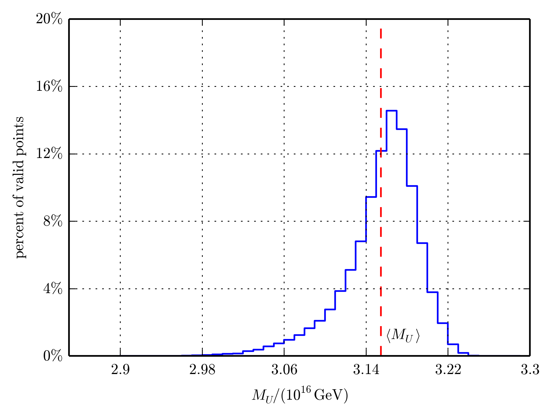

The results presented in Figures 5 and 6 lead us to postulate two new “phenomenological” constraints on our MSSM vacuum. The first constraint, arising from Figure 5, is that
| (5.6) |
Hence, given a point in the unity gauge Kähler moduli space shown in Figure 4 – and using (2.8) to compute the value of at that point – it follows from (5.6) that one can determine the required value of . Up to this point in the paper, was unconstrained. To elucidate the second constraint, we must present the explicit expression for the effective Lagrangian for the observable and hidden sector gauge field kinetic terms. This was calculated in [3, 4, 5] and, ignoring gravitation, was found to be
| (5.7) |
where is a parameter given by** * As discussed in [71], the expression for presented here is two times larger than the result given in [3, 4, 5].
| (5.8) |
For the specific choice of the hidden sector line bundle with embedding coefficient , the functions and in unity gauge are found to be
| (5.9) |
and
| (5.10) |
where and are given in (4.9) and (4.16) respectively. It then follows from Figure 6 and (5.7) that
| (5.11) |
Hence, given a point in the unity gauge Kähler moduli space shown in Figure 4 – and using (5.9) to compute the value of at that point – it follows from (5.11) that one can determine the required value of , which, up to this point, was unconstrained.
Using the relations
| (5.12) |
where and are the four-dimensional Newton’s constant and Planck mass respectively, it follows from (5.8) that
| (5.13) |
Finally, using these relations, the expression for in (3.4) can be rewritten as
| (5.14) |
That is, at any given fixed point in the unity gauge Kähler moduli space shown in Figure 4, which, by definition, satisfies all of the MSSM “vacuum constraints” listed in Sections 3 and 4, as well as the two “phenomenological” constraints presented in this subsection, one can determine all constant parameters of the theory – that is, , , , and . We again emphasize, as discussed above, that the unity gauge solution space of the vacuum constraints is valid for any arbitrary choice of .
5.2.2 Simultaneous Wilson lines
In the previous subsection, we presented the phenomenological constraints for the “left-right” split Wilson line scenario. Here, we will again discuss the two phenomenological constraints, but this time in the scenario where the mass scales of the two Wilson lines and the “unification” scale are approximately degenerate. Although somewhat less precise than the split Wilson line scenario, this “simultaneous” Wilson line scenario is more natural in the sense that less fine-tuning is required. We refer the reader to [35] for details. In this new scenario, we continue to use the previous mass scale as the “unification” scale – since its mass is set by the scale of the gauge bundle – even though when the Wilson lines are approximately degenerate the low-energy gauge couplings no longer unify there. Rather, they are split at that scale by individual “threshold” effects. Since the full MSSM low energy theory now exists at , we will assume that soft supersymmetry breaking also occurs at that scale. As shown in [35], we find that there are 44,884 valid black points which satisfy all low-energy physical requirements – including the correct Higgs mass. Rather than statistical plots over the set of all phenomenological black points, as we did in Figures 5 and 6 for the previous scenario, here we present a single figure showing the running of the inverse parameters for the , , and gauge couplings. This is presented in Figure 7.

Note that in the analysis of Figure 7, we use the gauge group instead of and instead of , which is a minor redefinition of the charges, since this simplifies the renormalization group analysis. However, the averages over their gauge thresholds differs only minimally from the basis used in this paper. Furthermore, we will augment the results of Figure 7 with a more detailed discussion below which uses our standard basis.
As discussed in the previous paragraph, the first constraint in this new scenario is identical to constraint (5.6) above. That is,
| (5.15) |
Hence, given a point in the unity gauge Kähler moduli space shown in Figure 4 – and using (2.8) to compute the value of at that point – it follows from (5.15) that one can determine the required value of . To elucidate the second phenomenological constraint in this scenario, however, requires a further analysis. First note from Figure 7, which is computed for a single initial valid black point, that at the values of the parameters for each of the four gauge couplings are given by
| (5.16) | |||
| (5.17) |
respectively. Taking the average over these parameters, we find that for that specific valid black point,
| (5.18) |
However, to get a more generic value for the average at the unification scale , one can either: 1) repeat the same analysis as in Figure 7, statistically calculating over all 44,884 valid black points and finding the average of the results, or 2) use the following technique, which is unique to a string theory analysis. Since our observable sector comes from an heterotic string theory in ten dimensions, we will use the second analysis for simplicity.
To do this, we note that, at string tree level, the gauge couplings are expected to grand unify to a single parameter at a “string unification” scale
| (5.19) |
The string coupling parameter is set by the value of the dilaton, and is typically of . A common value in the literature, see for example [72, 73, 74], is which, for specificity, we will use henceforth. Therefore, we take and the string unification scale to be
| (5.20) |
respectively. Note that is approximately an order of magnitude larger than . Below however, the couplings evolve according to the renormalization group equations of MSSM effective field theory. This adds another scaling regime, , to those discussed previously. The effective field theory in this regime remains that of the MSSM, with the same renormalization group factors as between the breaking scale and . However, the gauge coupling renormalization group equations are now altered to
| (5.21) |
where the index runs over , the coefficients are given in [41] and, for simplicity, we have ignored the “string threshold” corrections calculated in [35]. Note that the one-loop running gauge couplings do not unify exactly at . Rather, they are “split” by dimensionless threshold effects. Using (5.20) and taking , one can evaluate the parameter for each of the four gauge couplings at the scale . We find that
| (5.22) | |||
| (5.23) |
and, hence, the average “unification” parameter at is given by
| (5.24) |
It follows that for the “simultaneous” Wilson line scenario, the second phenomenological constraint is altered to become
| (5.25) |
Hence, given a point in the unity gauge Kähler moduli space shown in Figure 4 – and using (5.9) to compute the value of at that point – it follows from (5.25) that one can determine the required value of , which, up to this point, was unconstrained.
6 A Solution of All the Constraints
In Section 4, we displayed the solutions to all of the MSSM “vacuum” constraints, valid for a hidden sector line bundle embedded as in (4.5) with for a single five-brane with its bulk space location fixed to be at . The intersecting region of Kähler moduli satisfying all of these constraints, computed in unity gauge, are shown in Figure 4. In Section 5, we introduced three additional constraints. One of these, which we refer to as the “reduction” constraint, is required for the consistency of the dimensional reduction from the eleven-dimensional theory down to five dimensions. The other two, which we call the “phenomenological” constraints, are necessary so that the grand unified group in the observable sector has the correct unification scale, , and the right value of the physical unified gauge parameter, , determined from the MSSM via a renormalization group analysis. In this section we want to find the subspace of the solution space presented in Figure 4, which, in addition, is consistent with the reduction constraint and the two phenomenological constraints presented in Section 5.
We begin by imposing the physical constraints. We demand that at every point in the region of Kähler moduli space shown in Figure 4, all parameters of the theory are adjusted so that and are fixed at the physical values presented in Section 5 – that is, the unification scale is always set to , whereas for breaking with split Wilson lines, , while for breaking with simultaneous Wilson lines . It follows from the physical constraint equations (5.6), and (5.11) and (5.25) that the values of and – and, hence, the remaining parameters , and – can be always be chosen so as to obtain the required values of and . However, different points in Figure 4 will, in general, require different values of these parameters to satisfy the physical constraints. In particular, this means that different points will correspond to different values of . As discussed at the end of Section 4, this interpretation is completely consistent with the moduli shown in Figure 4 solving all of the “vacuum” constraints. To make this explicit, one can invert constraint equations (5.6), (5.11) and (5.25) so as to express and explicitly as functions of , and the Kähler moduli. That is, expression (5.6) can be inverted to give
| (6.1) |
| (6.2) |
As first presented in (5.9), the function is given by
| (6.3) |
where and for split and simultaneous Wilson lines respectively. Inserting these expressions into (5.13), (5.14) and (5.5), one obtains the following expressions for , and respectively. We find that
| (6.4) |
and
| (6.5) |
Using these expressions, the parameters at any fixed point of the moduli space in Figure 4 can be calculated. Again, we note that these parameters change from point to point in Figure 4.
Next, we impose the dimensional reduction constraint. We require that (5.1) be valid; that is, the length of the orbifold interval should be larger than the average Calabi–Yau radius
| (6.6) |
Choosing any point in the Kähler moduli space of Figure 4, one can use (6.1), (6.2), (6.4) and (6.5) to determine the parameters , , and that satisfy the phenomenological constraints at that point. Also note, since we are working in unity gauge (4.11), that
| (6.7) |
Now, at that chosen point in Figure 4, insert the calculated values of , , and , as well the value of computed from (6.7), into the inequality (6.6) for the ratio of the dimensions. Scanning over all points in Figure 4, we will be able to find the subspace of that region of Kähler moduli space in which condition (6.6) is satisfied. That is, at any such a point, not only are all the “vacuum” constraints satisfied, but the “reduction” and “phenomenological” constraints are as well. There, of course, will be two such regions – one corresponding to the “split” Wilson line scenario and a second corresponding to the “simultaneous” Wilson line scenario. These regions are shown as the brown subspaces of Figure 8 (a) and (b) respectively.


One can go further and, by scanning over the brown subspace associated with each Wilson line scenario, find the numerical range of the ratio in each case. We find that
| (6.8) |
for the split Wilson line scenario and
| (6.9) |
for the simultaneous Wilson lines.
Finally, but importantly, we want to emphasize that all of the results of this and preceding sections have, thus far, been calculated in “unity” gauge; that is, choosing
| (6.10) |
This was possible because, as discussed in Section 4, all “vacuum” constraints remained form invariant under the scaling
| (6.11) |
where . However, it follows from this that if any point {} in Figure 4 satisfies all vacuum constraints, so will any point {}. Do any of these “scaled” moduli carry new information concerning both the reduction and the physical constraints? The answer to this is no, as we will now demonstrate.
Let us pick any point {} in Figure 4 and assume that the values of the parameters at that point are given by , , and obtained from expressions (6.1), (6.2), (6.4) and (6.5) respectively evaluated at this point. We now want to determine how each of these parameters changes under the scaling given in (6.11). To do this, one can again use the same equations (6.1), (6.2), (6.4) and (6.5), but now scaling the original point as in (6.11). To do this, we must know the scaling behavior of both and respectively. It follows from (2.8) that . However, to obtain the scaling behavior of , one must go back to (3.6) and recall that the terms in linear in the Kähler moduli are, generically, multiplied by the factor . Since this is set to 1 in unity gauge, it does not appear in expression (6.3). Hence, it follows from (6.11) that under scaling . Using these results, we find that
| (6.12) | |||
| (6.13) |
Note that, until now, we knew that scaling invariance required , but could not specify the scaling of parameter and the modulus individually. However, from the last term in (6.13) it follows that
| (6.14) |
It is now straightforward to insert these results into the expression for the ratio of the orbifold interval length/average Calabi–Yau radius. We find that the scaling of the individual parameters and moduli exactly cancel. That is, under the scaling given in (6.11) and (6.13)
| (6.15) |
We conclude from this that the -scaled point of any point in the brown regions of Figure 8 (a) and (b) continues to satisfy all the “vacuum” and “phenomenological” constraints and and has identical values for the orbifold interval length/average Calabi–Yau radius. For this reason, we find it sufficient to display the final results as the brown regions in Figure 8 (a) and (b) only.
7 Slope-Stability and Supersymmetry
Thus far, we have found the region of Kähler moduli space in which the bundle is slope-stable with vanishing slope, the five-brane class is effective, the squares of both gauge couplings are positive, the length of the orbifold is larger than the characteristic length scale of the Calabi–Yau threefold and the vacuum is consistent with both the mass scale and gauge coupling of grand unification in the observable sector.
Importantly, however, we still must satisfy two remaining conditions. First, it is necessary that the gauge connection associated with a hidden sector line bundle on the Calabi–Yau threefold be a solution of the Hermitian Yang–Mills (HYM) equations [75, 76] and, second, that the line bundle be such that the low-energy effective theory admits an supersymmetric vacuum. We will now analyze both of these remaining constraints. First, for specificity, we restrict the analysis to the particular line bundle discussed above; that is, embedded into as in (4.4) with coefficient . In addition, we choose as in (4.16). Following that, however, we will present a discussion of these constraints for a “generic” line bundle with the same embedding (4.2) into and . To carry out these analyses, it is first necessary to introduce the Fayet–Iliopoulos term associated with the hidden sector gauge group and to discuss the correction to both the Fayet–Iliopoulos term and the slope.
7.1 A Fayet–Iliopoulos Term and the Slope Correction
It follows from (A.39) that the Fayet–Iliopoulos term associated with a generic single line bundle and a single five-brane located at is given in “unity” gauge by
| (7.1) |
with the volume modulus and presented in (2.8) and (3.2) respectively and defined in (2.20). Note that the coefficient defined in (2.19) enters this expression both explicitly and via the five-brane class .
It is important to note – using (2.3), (2.11) and (A.5) – that the “classical” slope of the line bundle is given by†† † Note that this is not the same as the scaling factor of the previous section. From here onwards, will denote the slope.
| (7.2) |
that is, the first term in the bracket of (7.1). It follows that the remaining terms in the bracket, specifically
| (7.3) |
are the strong coupling corrections to the slope of . For the remainder of this paper, we will take the slope of the line bundle to be the , genus-one corrected expression
| (7.4) |
7.2 Slope-Stability of the Hidden Sector Bundle
Although any line bundle is automatically slope-stable, since it has no sub-bundles, in order for its gauge connection to “embed” into the hidden sector gauge connection it is necessary to extend the bundle to , as discussed in subsection 4.2. However, even though the connection associated with the bundle can, in principle, embed properly into the gauge connection of the hidden sector , it remains necessary to show that is “slope-stable”; that is, that its associated connection satisfies the Hermitian Yang–Mills equations. More properly stated, since is the Whitney sum of two line bundles, it was shown in [75, 76] that it will admit a connection that uniquely satisfies the Hermitian Yang–Mills equations if and only if it is “polystable”; that is, if and only if
| (7.5) |
Since must vanish by construction, it follows that is polystable if and only if .
Let us now consider the specific line bundle embedded into as in (4.4) with coefficient , and take . It follows from (7.1) that in this case
| (7.6) |
and from (7.4) that the associated genus-one corrected slope is
| (7.7) |
Hence, this specific hidden sector bundle will be slope polystable – and, therefore, admit a gauge connection satisfying the corrected Hermitian Yang–Mills equations – if and only if the Kähler moduli satisfy the condition that
| (7.8) |
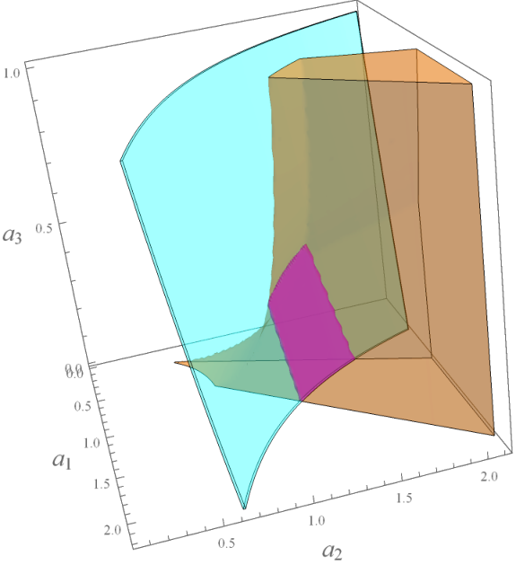
The region of Kähler moduli space satisfying this condition is the two-dimensional surface displayed in Figure 9.

Recall that for hidden sector line bundle with and for a single five-brane located at , the region of Kähler moduli space satisfying all previous constraints – that is, the slope-stability conditions, the anomaly cancellation constraint, the positive squared gauge coupling constraints, in addition to the dimensional reduction and the phenomenological constraints – are shown as the brown regions in Figure 8 (a) and (b), for the split Wilson lines and the simultaneous Wilson line scenarios respectively. It follows that the intersection of the brown regions of Figure 8 (a) and (b) with the the two-dimensional surface in Figure 9 will further constrain our theory so that the hidden sector gauge connection satisfies the corrected Hermitian Yang–Mills equations – as it must. The regions of intersection are displayed graphically in Figure 10. We emphasize that although the brown regions of Figure 8 (a) and (b) overlap in this region of Kähler moduli space, each point in their overlap region has a somewhat different set of parameters associated with it. Hence, in discussing a point in the magenta region of Figure 10, for example, it is necessary to state whether it is arising from the split Wilson line or simultaneous Wilson line scenario.
As we did previously for the brown regions presented in Figure 8 (a) and (b), it is of interest to scan over the magenta subspace of Figure 10 to find the numerical range of the ratio . We find that
| (7.9) |
for the split Wilson line scenario and
| (7.10) |
for simultaneous Wilson lines. In fact, one can go further and present a histogram of the percentage versus the ratio for each scenario. These histograms are shown in Figure 11 (a) and (b) for the split Wilson line and simultaneous Wilson line scenarios respectively.
Before proceeding to the discussion of supersymmetry in the effective theory, it will be useful to present the formalism for computing the low energy matter spectrum associated with a given hidden sector line bundle. We do this in the next subsection, displaying the formalism and low energy spectrum within the context of the line bundle for specificity.
7.3 The Matter Spectrum of the , Effective Theory
Having found the explicit sub-region of Kähler moduli space that satisfies all required constraints for the line bundle, in this subsection we will discuss the computation of the vector and chiral matter content of the low-energy theory of the hidden sector. Generically, the low-energy matter content depends on the precise hidden sector line bundle under consideration, as well as its embedding into . In this subsection, we again choose the line bundle to be , embedded into as in (4.5) with . However, the formalism presented is applicable to any line bundle with any embedding into . The commutant of the structure group of our specific embedding is . As discussed in Section 4, the decomposes under as
| (7.11) |
The corresponds to the adjoint representation of , while the give rise to chiral matter superfields with charges transforming in the representation of in four dimensions. The are singlet chiral superfields fields with charges under . Finally, the gives the one-dimensional adjoint representation of the gauge group. The embedding of the line bundle is such that fields with charge are counted by , charge fields are counted by and so on.‡‡ ‡ This is due to the form of the gauge transformation of the matter fields specified in (B.10). This was chosen so as to agree with [77, 78].
The low-energy massless spectrum can be determined by examining the chiral fermionic zero-modes of the Dirac operators for the various representations in the decomposition of the . Generically, the Euler characteristic counts , where and are the number of right- and left-chiral zero-modes respectively transforming under the representation associated with the bundle . With the notable exception of , which is discussed below, paired right-chiral and left-chiral zero-modes are assumed to form a massive Dirac fermion and are integrated out of the low-energy theory. Therefore, it is precisely the difference of the number of right-chiral fermions minus the left-chiral fermions, counted by the Euler characteristic , that give the massless zero-modes of the theory. On a Calabi–Yau threefold , can be computed by the Atiyah–Singer index theorem as
| (7.12) |
where are the dimensions of the -th cohomology group, is the Chern character of , and is the Todd class of the tangent bundle of . When is a line bundle, this simplifies to
| (7.13) |
Unlike the case of an bundle, when is a line bundle with non-vanishing first Chern class, can receive contributions from all four , . For example, then counts the number of (left-handed) chiral multiplets while counts (right-handed) anti-chiral multiplets, both transforming in the representation. Note that the multiplets counted by are simply the CPT conjugate partners of those already counted by . Since it is conventional to give a supersymmetric matter spectrum in terms of (left-handed) chiral supermultiplets, it is sufficient to compute for the various bundles under consideration.
Using (7.13), it is straightforward to compute the value of for the powers of associated with the decomposition (7.11). These are presented in Table 1. Having done this, let us discuss the spectrum in more detail.§§ § See [8], for example, for a similar discussion of the hidden-sector spectrum for an bundle.
| Cohomology | Index | |
|---|---|---|
- •
The index of the bundle associated with the and representations vanishes, so the corresponding fermionic zero-modes must be non-chiral. As discussed in [60], since the trivial bundle has and zero otherwise, there is a single right-chiral fermionic zero-mode (counted by ) and a single left-chiral fermionic zero-mode (counted by ), which combine to give the conjugate gauginos in a massless vector supermultiplet. In other words, the low-energy theory has one vector supermultiplet transforming in the adjoint representation of and one vector supermultiplet in the adjoint representation of .
- •
The multiplets are counted by . Since , there are 8 unpaired left-chiral fermionic zero-modes that contribute to 8 chiral matter supermultiplets transforming in the of .
- •
Similarly, the multiplets are counted by . Since , there are 8 unpaired right-chiral fermionic zero-modes that contribute to 8 anti-chiral matter supermultiplets transforming in the of . However, these do not give extra fields in the spectrum: they are (right-handed) anti-chiral supermultiplets which are simply the CPT conjugate partners of the 58 chiral supermultiplets already counted above [79].
- •
Since , there are 58 unpaired left-chiral fermionic zero-modes that contribute to 58 chiral matter supermultiplets transforming in the representation of .
- •
Similarly, the multiplets are counted by . Since , there are 58 unpaired right-chiral fermionic zero-modes that contribute to 58 charged anti-chiral matter supermultiplets transforming in the representation of . However, as discussed above, these do not give extra fields in the spectrum: they are (right-handed) anti-chiral supermultiplets which are simply the CPT conjugate partners of the 58 chiral supermultiplets already counted above.
In summary, the hidden sector massless spectrum for is
| (7.14) |
corresponding to one vector supermultiplet transforming in the adjoint representation of , one adjoint representation vector supermultiplet, eight chiral supermultiplets transforming as and 58 chiral supermultiplets transforming as .
Note that since we have a chiral spectrum charged under with all positive charges, the gauge symmetry will be anomalous. As we discuss in the next subsection, this anomaly is canceled by the four-dimensional version of the Green–Schwarz mechanism which, in addition, gives a non-zero mass to this “anomalous” hidden sector .
7.4 Effective Lagrangian and the Anomalous Mass
Before proceeding to the discussion of supersymmetry, it will be useful to present the effective theory for the hidden sector and to explicitly compute the anomalous mass of the gauge boson. We present the results for a generic hidden sector line bundle with an arbitrary embedding into the hidden sector . However, we conclude subsection 7.4.2 by computing the anomalous mass associated with the specific line bundle embedded into as in (4.5) with .
7.4.1 Effective Lagrangian
Following the conventions of [80, 81], the relevant terms in the four-dimensional effective action for the hidden sector of the strongly coupled heterotic string are
| (7.15) |
where denote the scalar components of the charged zero-mode chiral superfields, generically with different charges discussed in the previous subsection, are the complex scalar components
| (7.16) |
of the Kähler moduli superfields, where the are defined in (A.23) and are the associated axions, and is the hidden sector four-dimensional field strength. The Kähler metrics and are functions of the dilaton and Kähler moduli with positive eigenvalues. As we will see below, the exact form of is not important in this paper, whereas the exact form of will be essential in the calculation of the anomalous vector superfield mass. An explicit calculation of is presented in Appendix C. Note that we have written the kinetic term for the hidden sector gauge field as a trace over instead of using (B.12), so that . The final term in (7.15) is the potential energy, where is proportional to the solution of the auxiliary D-field equation of motion and is given by
| (7.17) |
The complex scalar fields enter the expression for since they transform linearly under with charge . Following (7.1), is the genus-one corrected Fayet–Iliopoulos term, which is associated with a single line bundle and a single five-brane located at . In “unity” gauge, where , it is given by
| (7.18) |
with the volume modulus and presented in (2.8) and (3.2) respectively.
7.4.2 The Anomalous Mass
As is commonly known, a symmetry that appears in the both the internal and four-dimensional gauge groups is generically anomalous [82, 83, 84, 85]. Hence, there must be a Green–Schwarz mechanism in the original heterotic M-theory which will cancel this anomaly in the effective field theory. Importantly, however, in addition to canceling this anomaly, the Green–Schwarz mechanism will give a mass for the vector superfield [86]. This occurs as follows. The Green–Schwarz mechanism leads to a non-linear action on the axionic partners of the Kähler moduli. That is, under a gauge transformation, one finds that
| (7.19) |
where the and parameters are defined in (3.4) and (5.5) respectively, is the parameter associated with the embedding of the line bundle into and is a gauge parameter. It follows that to preserve gauge invariance, the kinetic energy term for the complex Kähler moduli must be written with a covariant derivative of the form
| (7.20) |
Inserting this into the kinetic energy term for the moduli in (7.15), and scaling the gauge connection so that its kinetic energy term is in the canonical form , generates a mass for the vector superfield given by
| (7.21) |
The subscript refers to the fact that this mass arises from the Green–Schwarz mechanism required to cancel the gauge anomaly in the effective field theory. Using (C.3), (C.4) and (C.5), one can evaluate the metric , which is presented in (C.6). Inserting this into (7.21) leads to an expression for of the form
| (7.22) |
which is valid for a generic line bundle embedded arbitrarily into the hidden sector .
We conclude this subsection, by evaluating (7.22) for the specific line bundle embedded into as in (4.5) with . We display in Figure 12 the value of versus the ratio of the five-dimensional orbifold length to the average Calabi–Yau radius at different points across the magenta region shown in Figure 10 for both the split and simultaneous Wilson line scenarios.
7.5 Supersymmetric Vacuum Solutions in Four Dimensions
The generic form of the D-term in the four-dimensional effective theory for an arbitrary hidden sector line bundle was presented in (7.17). Using this result, we will now discuss the conditions for unbroken supersymmetry in the four-dimensional theory.
supersymmetry will be preserved in the effective theory only if the term presented in (7.17) vanishes at the minimum of the potential energy; that is
| (7.23) |
Whether or not the effective theory can satisfy this condition, and the exact details as to how it does so, depends strongly on the value of the Fayet–Iliopoulos term. There are two generic possibilities.
-
(i) The genus-one corrected FI-term vanishes. In this case, the VEVs of the scalar fields either all vanish or the VEVs of those fields with opposite charge, should they exist, cancel against each other.
-
(ii) The genus-one corrected FI-term is non-vanishing. In this case, non-zero VEVs of the scalar fields with the same sign as turn on to cancel the non-vanishing FI-term.
Each of the two scenarios comes with its own conditions which have to be met. In the first case, in order to obtain a vanishing FI-term, the strong coupling corrections to the slope need to cancel the tree-level “classical” slope in (7.18). For that to happen, one needs to be in a very strongly coupled regime, where working only to order may be a poor approximation. We provide a detailed discussion about the strong coupling expansion to first and higher order in Appendix D. In the second case, the low-energy spectrum needs to contain scalars with the correct charge under , such that their VEVs can cancel the non-zero contribution. In such a scenario, one can move in Kähler moduli space–while still satisfying all the vacuum and phenomenological constraints (that is, generically, outside the magenta region of Figure 10 while remaining within the brown region)–to a less strongly coupled regime in which the first-order expansion to is more accurate. However, as we will show in Section 7.5.2, the VEVs of these scalar fields may deform the hidden sector line bundle to an bundle, which might or might not be slope-stable.
7.5.1 Vanishing FI
Let us start by analyzing the first case. A simple way to ensure unbroken supersymmetry in and slope stability of the hidden sector bundle is to require that
| (7.24) |
There are then two scenarios in which supersymmetry can remain unbroken in the low energy theory. These are the following:
- 1.
The first, and simplest, possibility is that the charges of the scalar fields are all of the same sign. It follows that the potential energy will set all VEVs to zero, , and hence will vanish at this stable vacuum. Thus supersymmetry will be unbroken.
- 2.
A second possibility is that some of the signs may differ. This will lead to unstable, flat directions where both and the potential energy vanish. If one is at an arbitrary point, away from the origin, in a flat direction, then at least two VEVs will be non-vanishing and, hence, although preserving supersymmetry, such a vacuum would also spontaneously break the symmetry. In such a scenario, the non-zero VEVs of the scalars give a mass to the vector field via the super-Higgs effect. Scaling the gauge connection so that its kinetic energy term is in the canonical form , the value of this mass is easily computed and found to be
(7.25)
Having discussed this second possibility, we note again that the associated potential energy must have at least one flat direction and, hence, is an unstable vacuum state. For this reason, we will ignore such vacua in this paper. However, the first scenario is easily satisfied, as we now demonstrate with an explicit example.
Example: Supersymmetry for
We now discuss supersymmetry in the example introduced above, where the line bundle is taken to be and embedded into as in (4.4) with coefficient , and the location of the single five-brane is at . Recall that the genus-one corrected FI-term for this line bundle and embedding was presented in (7.6) and given by
| (7.26) |
In Figure 10, the region of Kähler moduli space which satisfies all of the required constraints, including slope stability, was presented. As discussed in detail in subsection 7.2, in order for the bundle to be polystable, it was necessary to restrict this region of moduli space to points that set the genus-one corrected slope (7.7) – and, hence, the FI-term in (7.26) – to zero. Furthermore, the low-energy scalar spectrum carrying non-vanishing charge was determined in subsection 7.3. It was shown there that the low-energy scalar spectrum of the hidden sector – specifically – each had charges of the same sign. It then follows from the above discussion that the potential energy must have a unique minimum where the VEVs vanish, , such that at this minimum. Hence, supersymmetry is unbroken in the vacuum state of the effective theory. Since the VEVs of all light charged scalar fields vanish for this explicit example, it follows from (7.25) that
| (7.27) |
However, as discussed above, since the symmetry is anomalous, the mass presented in (7.22) is non-vanishing and, for this explicit example, plotted in Figure 12.
We would like to point out that is not the only hidden sector line bundle which, if embedded into as in (4.5) with , has a region of Kähler moduli space where all required constraints are satisfied, and the vacuum preserves supersymmetry. However, any such line bundle must be “ample”–that is, each of its defining integers where must either be all positive or all negative. The reason is that for the Schoen manifold defined in Section 2, one can show that the genus-one corrected Fayet-Iliopoulos term can vanish, that is, , if and only if is ample. Restricting to ample line bundles, one can indeed find a significant number satisfying all required constraints. However, of these, many have a large number of equal sign zero-mode chiral multiplets – some with large charges –making them incompatible with spontaneous supersymmetry breaking via gaugino condensation. While potentially of physical interest, we wish to focus on the subset of ample line bundles that have a sufficiently small zero-mode chiral spectrum, with sufficiently small charges, to be compatible with supersymmetry breaking via gaugino condensation. These line bundles are specified by
| (7.28) |
and their duals; that is, for example, . Spontaneous supersymmetry breaking via gaugino condensation in this context will be explored in a future publication.
As discussed at the beginning of this section, although this hidden sector vacuum satisfies all required physical and phenomenological constraints, setting the FI-term to zero necessitates exact cancellation of the genus-one corrected slope against the tree-level slope of the hidden sector line bundle. Unsurprisingly, this fine-tuning can only be carried out in a relatively strongly coupled regime of heterotic M-theory – thus making the validity of the linearized approximation used in this paper uncertain. This is made more explicit and discussed in detail in Appendix D. It is, therefore, of some interest to explore vacua for which the genus-one corrections to the slope are significantly smaller than the tree level slope of the hidden sector bundle. In this case, one expects the effective coupling parameter to be smaller than in the previous scenario and, hence, the linearized results used in this paper to be a better approximation. For this reason, we now introduce the basic criteria required by hidden sector vacua where the FI-term does not vanish. Explicit examples of such hidden sector vacua will be presented in a future publication.
7.5.2 Non-vanishing FI
We now consider what happens when the correction to the tree-level slope is small and so cannot be used to set the FI-term to zero. The question then is, given a non-vanishing FI-term
| (7.29) |
can one still preserve supersymmetry in the four-dimensional effective theory?
Recall that the conditions for a supersymmetric vacuum are the vanishing of the F- and D-terms. For consistency with the previous content of this paper, let us continue to assume that the vacuum has an unbroken gauge symmetry, embedded into as discussed in Section 4.2. It follows that the D-terms will vanish by setting the VEVs of the non-abelian matter fields to be zero. Any F-terms involving the non-abelian matter fields will then also vanish. As discussed in [87], the F-term conditions for the matter fields permit us to give VEVs to only one set of fields, that is, either or but not both. The remaining condition for the vacuum solution to be supersymmetric is the vanishing of the D-term, . Since the term does not vanish for any choice of line bundle when the correction is small, one is forced to cancel the term against the VEVs of the charged singlet fields. In other words, we want
| (7.30) |
Obviously, such a cancellation will depend on the relative sign of and the charges of the scalars . For example, if the term is positive, one needs at least one zero-mode chiral supermultiplet whose scalar component is a singlet under the non-abelian group and has positive charge. Whether or not such scalar fields are present will depend on the specific line bundle studied.
If one can cancel the FI-term in this way, the non-zero VEVs of the scalars give a mass to the vector field via the super-Higgs effect:
| (7.31) |
where the subscript indicates that this mass is due to the non-vanishing VEVs needed to set the D-term to zero. Note that in the case where one gives VEVs to fields of a single charge , the mass is related to the term as
| (7.32) |
As in the case of vanishing slope in the previous subsection, the vector field mass also receives a contribution from the Green–Schwarz mechanism. Hence the total mass of the vector field is given by the sum of above and from (7.22).
As we discussed in Section 4.2, the embedding of inside that we have considered for much of this paper factors through the subgroup of that commutes with . The gauge connection for the line bundle can be thought of as defining an connection in two equivalent ways: either embedding directly in via the generator discussed around (4.5), or first embedding in as and then embedding in via (4.3). The second of these two pictures is helpful for understanding the effect of allowing non-zero VEVs for the charged singlets, .
First note that the connection is a connection for an bundle which splits as a direct sum
| (7.33) |
of line bundles. How does this relate to supersymmetry? The induced connection will solve the (genus-one corrected) Hermitian Yang–Mills equation, and so give a supersymmetric solution, if the connection itself solves the (genus-one corrected) Hermitian Yang–Mills equation. This is guaranteed if the rank two bundle is polystable with vanishing slope.¶¶ ¶ Here, slope is taken to mean the genus-one corrected slope. The same comments apply if one considers only the tree-level expression. Since by construction, the remaining conditions for polystability are
| (7.34) |
This is exactly the vanishing case studied in 7.5.1, where the corrected slope of is set to zero and the VEVs of the charged singlet matter fields vanish.
When , the bundle is no longer polystable and so its connection does not solve the Hermitian Yang–Mills equation. The four-dimensional consequence of this is that the term no longer vanishes. However, we might be able to turn on VEVs for appropriate charged singlet matter fields in order to cancel the term and set the D-term to zero, thus preserving superysymmetry. One might wonder: what is the bundle interpretation of turning on VEVs for these charged singlet matter fields? As discussed in [88, 89, 90], these VEVs should be seen as deforming the gauge bundle away from its split form to a non-split bundle which admits a connection that does solve the Hermitian Yang–Mills equations.
Consider the case where (equivalent to ) in some region of Kähler moduli space where the constraints of Section 4 are all satisfied. From (7.30) we see that one can set provided we have charged scalars with positive charge, . From the generic form of the cohomologies in Table 1, the required scalars are those transforming in , with the chiral superfields which contain these scalars counted by . Hence, giving VEVs to scalars corresponds to allowing non-trivial elements of . The first summand has an interpretation as the space of extensions of by , with the exact sequence
| (7.35) |
defining an bundle . This extension can be non-trivial () provided
| (7.36) |
Choosing a non-zero element of this space then corresponds to turning on VEVs for some set of scalars. Thus we see that giving VEVs to positively charged singlet scalars arising from amounts to deforming the induced bundle to the bundle . Note that if , the VEVs of positively charged matter coming from cannot be interpreted as deforming to a new bundle. Hence, the bundle remains which is unstable and, therefore, its gauge connection does not solve the Hermitian Yang–Mills equation.
Assuming one can show for a given line bundle that , it might seem that we are done – the D-term vanishes and supersymmetry appears to have been restored. However, the four-dimensional analysis is insensitive to whether the new bundle is slope stable and thus actually admits a solution to Hermitian Yang–Mills. Unfortunately, checking slope stability is a difficult calculation that one must do explicitly for each example. As a preliminary check, one can first see whether satisfies some simpler necessary conditions for slope stability. First, the obvious subbundle should not destabilise . In our case this is guaranteed as we have assumed , so that has negative slope.∥∥ ∥ If instead , one simply swaps the roles of and in the above discussion and instead considers the extension of by . Second, must satisfy the Bogomolov inequality [91]. For a bundle with vanishing first Chern class, this states that if is slope stable with respect to some choice of Kähler class , then
| (7.37) |
Since is constructed as an extension of line bundles, we have
| (7.38) |
with . Thus if is to be slope stable, we must be in a region of Kähler moduli space where
| (7.39) |
Note that this is a necessary but not sufficient condition. However, it is often the case that the Bogomolov inequality is the only obstruction to finding stable bundles [57].
We thus have a new set of necessary conditions on (in addition to the physically and mathematically required constraints presented in Section 4) for there to be a supersymmetric vacuum after turning on the VEVs to cancel the FI-term. These are
- 1.
Singlet matter with the correct charge must be present, so that can be canceled and the D-term set to zero.
- 2.
must not vanish.
- 3.
The Bogomolov inequality, , must be satisfied.
Does our previous choice of satisfy these conditions? Note that everywhere in the Kähler cone for this line bundle. From its low-energy spectrum in Table 1, we see we have 58 massless positively charged singlets transforming in the representation, and so we do indeed have the correct matter to cancel the FI-term and set the D-term to zero. However, as discussed in [60], if is an ample line bundle then
| (7.40) |
Since –and, hence, –is ample, it follows that . Therefore, condition 2 above implies that cannot admit an extension to an bundle . Ignoring this for a moment, and assuming that there did exist an extension, we would still have to check whether or not the Bogomolov inequality, a necessary condition for to be slope stable, is satisfied. However, from (7.39) and the positivity of the Kähler moduli, we see that it is impossible to satisfy this inequality, implying (again) that the split bundle constructed from cannot be deformed to admit a solution to the Hermitian Yang–Mills equation. Moreover, we see the same will be true for any ample line bundle – the are positive and is not satisfied anywhere in the positive Kähler cone.
What about other choices of line bundle? It turns out that of the three conditions, the Bogomolov inequality is the more difficult to satisfy. Scanning over different choices of , one finds that in the region of Kähler moduli space where the bundle is stable, the only line bundles that are equivariant with ,**** ** We restrict to in our scan to match our analysis above. Including bundles with would give the reverse extension sequence with the bundle and its dual swapped, leading to the same bundles that were already captured by restricting to positive slope. allow for anomaly cancellation and satisfy the Bogomolov inequality are
| (7.41) |
Do any of these have positively charged singlet matter in their low-energy spectrum to allow for a non-trivial extension? That is, do we have for any of these candidate line bundles? For and , it is simple to show using a Leray spectral sequence that the answer is no. For a definitive answer in the remaining two cases, one must extend the analysis of Appendix A of [57] to higher degree line bundles on dP9. This is beyond the scope of the present paper. Therefore, for now, we content ourselves with noting that is positive for both remaining line bundles, which is consistent with and the absence of an extension to a bundle .
As exploited by a number of other works [87, 13, 15], moving from a single line bundle to two or more such bundles provides a richer low-energy spectrum, making it much easier to find examples which possess the correct charged matter and satisfy both the phenomenological constraints and the Bogomolov inequality. We intend to pursue this in detail in future work.
8 Conclusions
In this paper, we have explicitly chosen the hidden sector line bundle , embedded in a specific way with embedding coefficient into the gauge group, and studied its phenomenological properties. This choice of hidden sector was shown to satisfy all “vacuum” constraints required to be consistent with present low-energy phenomenology, as well as both the “reduction” and “physical” constraints required to be a “strongly-coupled” heterotic vacuum consistent with both the mass scale and gauge coupling of a unified theory in the observable sector. Additionally, we showed that the induced bundle is polystable after including genus-one corrections, and that the effective low-energy theory admits an supersymmetric vacuum. We pointed out that there are actually a large number of different line bundles that one could choose, and a large number of inequivalent embeddings of such line bundles into . An alternative choice of hidden sector bundle could lead to: 1) a different commutant subgroup and hence a different low-energy gauge group, 2) a different spectrum of zero-mass particles transforming under , 3) a different value for the associated Fayet–Iliopoulos term and, hence, a different D-term mass for the vector superfield, and so on. Furthermore, a richer zero-mode spectrum could open the door to mechanisms for arbitrary size spontaneous supersymmetry breaking, new dark matter candidates and other interesting phenomena. We will explore all of these issues in several upcoming papers.
Acknowledgements
We would like to thank Yang-Hui He and Fabian Ruehle for helpful discussions. Anthony Ashmore and Sebastian Dumitru are supported in part by research grant DOE No. DESC0007901. Burt Ovrut is supported in part by both the research grant DOE No. DESC0007901 and SAS Account 020-0188-2-010202-6603-0338.
Appendix A Vacuum Constraints for Strongly Coupled Heterotic M-Theories
The required vacuum constraints for heterotic M-theories, in the context of both weak and strong coupling, have been discussed in several previous papers [60, 59]. In particular, the explicit constraints involving both the observable and hidden sectors for phenomenologically realistic strongly coupled heterotic M-theory vacua were presented in detail in [59]. Since these form the starting point for the analysis in the present work, in this Appendix we will briefly list the important definitions, summarize the relevant results and emphasize the physically pertinent conclusions contained in [59].
A.1 The Hidden Sector Bundle
In [59], the hidden sector vector bundle was chosen to have the generic form of a Whitney sum
| (A.1) |
where is a slope-stable, non-abelian bundle and each , is a holomorphic line bundle with structure group . However, in this Appendix, we will restrict our discussion to hidden sector gauge bundles of the form
| (A.2) |
Being a Whitney sum of line bundles, must be polystable – that is, each line bundle must have the same slope which is, however, prior to a discussion of supersymmetry in the low energy theory, otherwise unrestricted.
A.1.1 Properties of Hidden Sector Bundles
It follows that form of the hidden sector bundle will be
| (A.3) |
where
| (A.4) |
for any positive integer . The structure group is , where each factor has a specific embedding into the hidden sector gauge group. It follows from the definition that that the first Chern class is
| (A.5) |
Note that since is a sum of holomorphic line bundles, . However, the relevant quantity for the hidden sector vacuum is the second Chern character defined in [59]. For this becomes
| (A.6) |
Since , it follows that
| (A.7) |
where
| (A.8) |
with the generator of the -th factor embedded into the adjoint representation of the hidden sector , and the trace is taken over the of (including a conventional factor of ).
A.2 Anomaly Cancellation
As discussed in [5, 92], anomaly cancellation in heterotic M-theory requires that
| (A.9) |
where
| (A.10) |
Note that the indices and denote the observable and hidden sector domain walls respectively, and not the location of a five-brane. Using the definitions of the associated Chern characters, the anomaly cancellation condition can be expressed as
| (A.11) |
where we have restricted the hidden sector bundle to be of the form (A.3) and is the total five-brane class. Furthermore, it follows from the properties of the Chern characters, and defining
| (A.12) |
that the anomaly condition (A.11) can be expressed as
| (A.13) |
The positivity constraint on follows from the requirement that it be an effective class to preserve supersymmetry.
A.3 The Linearized Double Domain Wall
The five-dimensional effective theory of heterotic M-theory, obtained by reducing Hořava–Witten theory on the above Calabi–Yau threefold, admits a BPS double domain wall solution with five-branes in the bulk space [4, 93, 5, 24, 18, 3]. This solution depends on the moduli and defined in the text, as well as the , functions of the five-dimensional metric
| (A.16) |
all of which are dependent on the five coordinates , of . Denoting the reference radius of by , then . The detailed structure of the linearized double domain wall depends on the solution of three non-linear equations discussed in [5]. These can be approximately solved by expanding to linear order in the quantity , where we define with , is given in (A.15) and
| (A.17) |
The parameters and are defined in the text and is the dimensionful eleven-dimensional Planck constant. It is also convenient to express the moduli of the theory in terms of orbifold average functions defined as follows. For an arbitrary dimensionless function of the five coordinates, define its average over the orbifold interval as
| (A.18) |
where is the reference length. Then is a function of the four coordinates , of only. The linearized solution is expressed in terms of orbifold average functions
| (A.19) |
The fact that they are averaged is indicated by the subscript .
The solution to these linearized equations depends on the number of five-branes located within the fifth-dimensional interval. Here, for simplicity, we will consider the vacuum to contain a single five-brane, wrapped on a holomorphic curve, and located at the fifth-dimensional coordinate . It was then shown in [5] that the conditions for the validity of the linear approximation then break into two parts. Written in terms of the averaged moduli, these are
| (A.20) |
and
| (A.21) |
When dimensionally reduced on this linearized BPS solution, the four-dimensional functions , , and will become moduli of the effective heterotic M-theory. The geometric role of and will remain the same as above – now, however, for the averaged Calabi–Yau threefold. For example, the dimensionful volume of the averaged Calabi–Yau manifold will be given by . The new dimensionless quantity will be the length modulus of the orbifold. The dimensionful length of is given by . Finally, since the remainder of this Appendix will be within the context of the effective theory, we will, for simplicity, drop the subscript on all moduli henceforth – as well as everywhere in the text of this paper.
A.4 The Effective Theory
When heterotic M-theory is dimensionally reduced to four dimensions on the linearized BPS double domain wall with five-branes, the result is, modulo the discussion below, an supersymmetric effective four-dimensional theory with (potentially spontaneously broken) gauge group. The Lagrangian will break into two distinct parts. The first contains terms of order in the eleven-dimensional Planck constant , while the second consists of terms of order .
A.4.1 The Lagrangian
This Lagrangian is well-known and was presented in [3]. Here we discuss only those properties required in this paper. In four dimensions, the moduli must be organized into the lowest components of chiral supermultiplets. Here, we need only consider the real part of these components. Additionally, one specifies that these chiral multiplets have canonical Kähler potentials in the effective Lagrangian. The dilaton is simply given by
| (A.22) |
However, neither nor – defined in (2.6) and (2.9) respectively – have canonical kinetic energy. To obtain this, one must define the re-scaled moduli
| (A.23) |
where we have used (2.9) in the text, and choose the complex Kähler moduli so that
| (A.24) |
Denote the real modulus specifying the location of the -th five-brane in the bulk space by where . As with the Kähler moduli, it is necessary to define the fields
| (A.25) |
These rescaled five-brane moduli have canonical kinetic energy.
A.4.2 The Lagrangian
The terms in the BPS double domain wall solution proportional to lead to order additions to the Lagrangian. These have several effects. The simplest is that the five-brane location moduli now contribute to the definition of the dilaton, which becomes
| (A.26) |
where the fields are defined in (A.23). More profoundly, these terms lead, first, to threshold corrections to the gauge coupling parameters and, second, to additions to the Fayet–Iliopoulos (FI) term associated with any anomalous factor in the low-energy gauge group. Let us analyze these in turn.
A.5 Gauge Threshold Corrections
The gauge couplings of the non-anomalous components of the gauge group, in both the observable and hidden sectors, have been computed to order in [24]. Written in terms of the fields defined in (2.9) and including five-branes in the bulk space, these are given by
| (A.27) |
and
| (A.28) |
respectively. The positive definite constant of proportionality is identical for both gauge couplings and is not relevant to the present discussion. It is important to note that the effective parameter of the expansion in (A.27) and (A.28), namely , is identical to the parameter appearing in (A.20) and (A.21)) for the validity of the linearized approximation with a single five-brane. That is, the effective strong coupling parameter of the expansion is given by
| (A.29) |
We point out that this is, up to a constant factor of order one, precisely the strong coupling parameter presented in equation (1.3) of [94].
Recall that and correspond to the observable and hidden sector domain walls – not to five-branes. Therefore, and . Using (A.10) and (A.14), one can evaluate the coefficients in terms of the the Kähler moduli defined in (2.6). Rewrite the above expressions in terms of these moduli using (2.8), (2.9), (A.6), (A.7), and redefine the five-brane moduli to be
| (A.30) |
Furthermore, choosing our hidden sector bundle to be that given in (A.2), we find that
| (A.31) |
and
| (A.32) |
where is given in (A.8). The first term on the right-hand side, that is, the volume defined in (2.8), is the order result. The remaining terms are the M-theory corrections first presented in [24].
A.6 Corrections to a Fayet–Iliopoulos Term
In the heterotic standard model vacuum, the observable sector vector bundle has structure group . Hence, it does not lead to an anomalous gauge factor in the observable sector of the low energy theory. However, the hidden sector bundle introduced above consists of a sum of line bundles with the additional structure group . Each factor leads to an anomalous gauge group in the four-dimensional effective field theory of the hidden sector and, hence, an associated -term. Let be any one of the irreducible line bundles of . The string one-loop corrected Fayet–Iliopoulos (FI) term for was computed in [85] within the context of the weakly coupled heterotic string, and in [95, 78] for a specific embedding of into in strongly coupled heterotic -theory. Comparing various results in the literature, it is straightforward to show that to order the one-loop corrected FI-term for in the strongly coupled heterotic string is
| (A.37) |
where is a group-theoretical coefficient, defined in (A.8), determined by how the structure group of embeds in , and is given in (2.11). We note that the part of this expression is identical to that derived in [78]. Insert (A.10) and, following the conventions of [85, 96], redefine the five-brane moduli as in (A.30). Furthermore, choosing our hidden sector bundle to be that given in (A.2), we find that the FI-term becomes
| (A.38) |
The first term on the right-hand side, that is, the slope of , is the order result. The remaining terms are the M-theory corrections first presented in [24]. Note that the dimensionless parameter of the term is identical to the expansion coefficient of the linearized solution – when expressed in term of the moduli. Finally, recalling definition (2.11) of the slope, using (2.3), (2.4), (2.6), (A.5), (A.12) and the properties of the second Chern character, it follows that for each the associated Fayet–Iliopoulos factor in (A.38) can be written as
| (A.39) |
where
| (A.40) |
Appendix B Gauge Transformations and the FI-Term
B.1 The Green–Schwarz Mechanism and the Axion Transformation
In heterotic M-theory, a gauge transformation of the Yang–Mills field leads to a transformation of the M-theory three-form. This transformation was used in [78] to derive the anomalous gauge transformation of the Kähler axions and the resulting D-term contribution to the four-dimensional potential. Since our structure group embeds into in a different fashion from that in [78], it is instructive to re-derive this transformation. Following the conventions of [80], the gauge-invariant four-form field strength is given by , where the Chern–Simons three-form is
| (B.1) |
and and satisfy
| (B.2) | ||||
| (B.3) |
Focusing on the second factor and dropping the subscript “2”, locally is given by the usual Chern–Simons three-form
| (B.4) |
where the dots indicate terms that contribute to and are not relevant to our discussion. The four-form is clearly gauge invariant under standard shifts by closed three-forms, . However, it is less obvious that is invariant under Yang–Mills gauge transformations. Under a gauge transformation of by , the four-form must be invariant. For this to be true, one must have From (B.4), it is straightforward to show that the transformation of is
| (B.5) |
Using the expressions for in (B.1) and , locally the gauge transformation of must be
| (B.6) |
where we have written this in components and specialized to an abelian gauge field, in agreement with [78].
The gauge transformation of the three-form leads to a gauge transformation of the Kähler axions via . Integrating this over , where the are dual to , then gives
| (B.7) |
When is the field strength of a non-abelian symmetry, the above expression for vanishes and so this does not result in a gauge transformation in four dimensions. Why is this? If is non-abelian and it has a non-zero VEV on the internal space, then the corresponding gauge group cannot appear as a four-dimensional gauge symmetry (since a non-abelian group does not commute with itself inside ), and so there is no symmetry group in four dimensions to have a gauge transformation with respect to. However, for a factor, these gauge transformations are present since the appears as a factor in both the internal and four-dimensional groups. Written in terms of the four-dimensional , the trace reduces to
| (B.8) |
where is the gauge parameter for the four-dimensional transformation and on the right-hand side is the internal field strength. Noting that this is identified with the structure group of the internal line bundle , we have , so that the gauge transformation of the axions can be written as†††† †† The four-dimensional in [78] is that which appears in the commutant of , leading to a different group-theoretic coefficient in .
| (B.9) |
We see that the four-dimensional gauge transformation of the Kähler axions is fixed by the strong coupling parameters and , together with the group-theoretic factor that characterizes how the embeds in the hidden . The gauge transformations of the axions imply a gauge transformation of the complexified Kähler moduli, defined by , where the are defined in (A.23).
The singlet matter fields also transform under the four-dimensional symmetry, with gauge transformations given by
| (B.10) |
where, for example, for the scalars of the superfields transforming as . Using these transformations rules, both the D-term and the mass of the can be derived by standard methods [77, 81].
B.2 Various Trace Relations
The kinetic terms for the gauge fields are naturally written as traces over the generators in the representation normalized with an extra factor of . For the visible sector, the four-dimensional gauge group is (broken down from by the bundle). Writing the visible sector curvature as , the and traces are related via
| (B.11) |
where the trace is taken in the fundamental representation, which is normalized so that . The four-dimensional gauge group in the hidden sector is the commutant of the inside . Generically this will be , where is a non-abelian factor, chosen to be for the majority of this paper. For the computation of the FI-term, we are interested only in the gauge field. Therefore, we should rewrite the trace over the generator specifying the embedding in in terms of the trace over the fundamental representation of instead. Tracing over we define
| (B.12) |
where we are taking as the generator of the fundamental representation of . For the embedding we use in this paper, one finds that .
Appendix C The Anomalous Mass Contribution
As we discuss in the main text, the mass of the vector field is
| (C.1) |
which can be expressed as
| (C.2) |
The first term appears because of the non-zero VEVs of the scalar fields which, if their charges are appropriate, could cancel the D-term in our four-dimensional theory. The second term is induced by the Green–Schwarz mechanism. To compute the second term, we need to know the metric . This is defined by
| (C.3) |
with the Kähler potential given by
| (C.4) |
where
| (C.5) |
Taking derivatives with respect to the complex scalars , we then find
| (C.6) |
Contracting this expression with , we then have
| (C.7) |
Putting this all together, we find an expression for of the form
| (C.8) |
Note that since the scale of the FI-term and, hence, for , is set by , the anomalous mass is suppressed by a factor of relative to .
Appendix D The BPS Vacuum Solution and the Linearization Constraints
D.1 The Strong Coupling Linearization Constraints
In (A.20) and (A.21) of Appendix A, the constraints required for the validity of the linearized approximation to the five-dimensional BPS solution of the Hořava–Witten theory are presented. These constraints are restricted to the case of a single five-brane located at . Reproducing the equations here, we have
| (D.1) |
and
| (D.2) |
where, as discussed in Appendix A, we have removed the subscript on the orbifold averaged moduli. Note that expressions (D.1) and (D.2) depend on the observable-sector gauge bundle and the bulk-space five-brane but are, however, independent of the gauge bundle on the hidden sector. In unity gauge and in terms of the Kähler moduli , the strong coupling constraints (D.1) and (D.2) simplify to
| (D.3) |
and
| (D.4) |
respectively, where .
As discussed in Appendix A.5 for the linearized expansion of the gauge threshold corrections, and defined in (A.29), the effective “strong coupling parameter” is given by
| (D.5) |
Note that this is precisely the moduli dependent parameter on the left-hand side of (D.1) and (D.2) above. By definition, the effective strong coupling expansion parameter is a reasonable measure of the validity of the linearized expansion of the various quantities used in this paper. It is important to note that in heterotic M-theory, where the observable and hidden sector orbifold planes are separated by the fifth-dimension, one expects the effective coupling parameter to become perturbatively small only when the walls are very close to each other. Even for a small separation on the order of a few times the average Calabi–Yau threefold radius, this parameter is fairly large, rapidly becoming a strong coupling parameter as the distance between the orbifold walls begins to significantly exceed the Calabi–Yau radius. That is, heterotic M-theory is, by definition, a strongly coupled theory. Be that as it may, very loosely speaking, when , one might expect the linear approximation used throughout this paper to be weakly valid. However, when , one is truly in a strongly coupled regime and the validity of the linearized approximation comes into doubt. As a check on this, we find that in the strongly coupled regime with the terms on the left and on the right sides of the expressions (D.1) and (D.2) are roughly of similar size. On the other hand, the left side is somewhat smaller than the right-hand side of these inequalities when .
The major result of this paper is the construction of a hidden sector for the “heterotic standard model”. The hidden sector consists of a line bundle , embedded into as in (4.4) with coefficient . In addition there is a single five-brane located at in the fifth-dimension. It was shown that for a significant region of Kähler moduli space, the induced rank two bundle of this hidden sector satisfied the required “vacuum” constraints, the reduction and phenomenological constraints (the brown regions of Figure 8 (a) and (b)), as well as being slope polystable and , supersymmetric (the magenta region of Figure 10). However, importantly, in order to satisfy the last two constraints – that is, slope poly-stability and , supersymmetry – it was necessary to be in the region of Kähler moduli space in which the associated Fayet–Iliopoulos term vanished. That is, . For this to be the case, it is necessary to exactly cancel the genus-one correction to the FI-term against its tree level value. In addition to the fine-tuning required, this clearly suggests that the parameter might be quite large. To determine this analytically, in Figure 13 (a) and (b) we plot both and against the ratio of the length of the fifth-dimension to the average Calabi–Yau radius for the brown regions of Figure 8 (a) and (b) – all of which can be determined for any point in the relevant Kähler moduli space. In each figure (a) and (b), the horizontal red line indicates when ; that is, when . We immediately see that to set , it is necessary for to take the values and for the split and simultaneous Wilson line scenarios respectively. That is, as expected, in both cases and, hence, one is in a strongly coupled regime where the linear expansion solution to the five-dimensional BPS state might not be a good approximation.
An alternative scenario, in which the FI-term does not vanish, would allow us to be in a less strongly coupled region where the linearity constraints (D.1) and (D.2) would be well-satisfied. This scenario was discussed in detail in Section 7.5.2, but was proven to be non-applicable to a hidden sector consisting of a single line bundle. This leaves the vanishing-slope scenario as the only viable option for obtaining a supersymmetric effective theory in the type of embedding into used in this paper.
As discussed in the text and Appendix A, the formalism in this paper is based on using the linear approximation to solve the five-dimensional BPS vacuum equations – first described in [5]. Although we find that the linear expansion is not sufficiently accurate in the case that we are interested in, heterotic M-theory has never been solved to include terms of orders higher than and . In the absence of an exact solution, accurate to all orders, we have no choice but to use the existing results in the literature, which are expansions to linear order. However, in the following, we will try to get an idea of how our equations and results might change if we were to work to one order higher than in this paper.
Our analysis follows the solution presented in [5], but we will extend it to one order higher. Note that the notation will be slightly changed. In [5], the BPS state equation
| (D.6) |
is solved to linear order only, with the ansatz
| (D.7) |
where and are constants which depend on the Kähler moduli averaged over the fifth dimension and is the space coordinate across the fifth dimension, defined as . Ideally, . We will assume the five-brane is very close to the hidden wall, that is, . In this limit, is given by the expression
| (D.8) |
We will now extend this analysis to second order and, hence, write
| (D.9) |
Since eleven-dimensional Hořava–Witten theory, as well as its reduction to a five-dimensional effective theory, are both valid only to order , it is unclear what going to even higher order in the solution of the BPS vacuum equation would mean. Be that as it may, it does give an indication of how various physical quantities might behave at higher order. Matching the powers of in equation (D.6) we obtain
| (D.10) |
Let us attempt to solve these equalities, making use of the fact, presented in [5], that
| (D.11) |
To second order in the dependence, these quantities can be expressed as
| (D.12) |
Matching the powers in at zeroth order, we can now proceed to evaluate , and . We find that
| (D.13) |
while is given by
| (D.14) |
and finally
| (D.15) |
Using , one can then compute the values of , , and to second order. For the volume and the metric functions and , we find
| (D.16) | ||||
| (D.17) | ||||
| (D.18) |
while for the moduli we simply have
| (D.19) |
One can further convert the shape moduli to the Kähler moduli via
| (D.20) |
The only thing left to do before one can compute how the volume , the metric moduli , and the Kähler moduli vary across the fifth dimension is to fix the constant . It follows from (D.18) that
| (D.21) |
In the theory, we can identify the averaged value of over the fifth dimension with . Furthermore, in the effective theory we know that we can go to unity gauge and set , where is the average of the volume over the fifth dimension. In our second order expansion, the tree level values of our moduli do not equal the average of these moduli over the fifth dimension. However, we will show that for and , one can approximate the tree level values in the Taylor expansions, and , to be equal to the effective theory values and . Hence, we set
| (D.22) |
and . In this limit, we find
| (D.23) |
which allows us to also determine exactly.
Having determined exactly, one can now evaluate how the volume , the metric functions and the Kähler moduli change as functions of the fifth dimensional coordinate . We are mainly interested in the region of Kähler moduli space, analyzed in the text, where, in addition to all necessary constraints being satisfied, the genus-one corrected FI-term also vanishes; that is, the magenta region of Figure 10. In order to compare our results to the linear case studied in [5], we will write the Taylor expansions around the center of the interval , which is equivalent to shifting
| (D.24) |
in (D.9). To determine how , , and behave for points within the solution space on which the FI-term vanishes–the magenta region of Figure 10–naively, one would choose a point within this solution space and compute the behavior of these functions. However, the solution space we found was in terms of the effective moduli . Here, where we work to order , one can only compute the functions , , and once we specify the zeroth-order values , which, in general, are not equal to the average of over the interval (unlike in the linear case). Therefore, our problem is that we can find if we are within the solution space or not only after we sample the values for , compute and do the average
| (D.25) |
For example, let us choose . From this, one can compute all coefficients specified above and, hence, as well as and and the coefficients for . We begin by plotting the the -dependent functions . They appear as the red lines in Figure 14 from left to right respectively. Taking the average (D.25) over each of these three functions, we find that . These values are plotted as the dashed green lines in Figure 14. We find that indeed sits on the surface of vanishing slope, that is
| (D.26) |
and is a point in the interior of the physical magenta region shown in Figure 10. It is of interest to compare the order solutions to the linear order results. To do so, we truncate the expansions in (D.12) at order and now, using the averaged values , compute all coefficients to linear order, that is, specified above and, hence, as well as and and the coefficients for . The linear order results are shown as the blue curves in Figure 14. The first thing to note is that the linearized approximations to and, more significantly, both become unacceptably negative in the interval . In particular, is deeply negative over much of the interval . However, we see that by going to order , is positive over the entire interval, while – although still slightly negative in the interval – is much less negative than in the linearized case and is clearly correcting the behavior of significantly.

.
As a second check on the relationship between the order and the linearized approximations, we now plot , and in both cases – using, as above, as the order-zero coefficients and as the order-zero linear approximation coefficients. These are plotted as the red and blue lines from left to right respectively in Figure 15. Among the conclusions we can draw from this second-order extended analysis is that the moduli and do not change much when including the second order corrections, even in the strongly coupled regime we have to work in. The behavior of is particularly encouraging, because it is directly related to the kinetic functions and , and hence, to the gauge couplings and on the observable and hidden sector, respectively. Our finding implies that the regions of validity for and do not change significantly.

Finally, we note that these results have been obtained under the assumption that can be approximated by . So was that approximation justified in our case? We find for and that
| (D.27) |
while
| (D.28) |
respectively. Hence, the approximation is well justified.
References
- [1] P. Horava and E. Witten, “Heterotic and type I string dynamics from eleven-dimensions”, Nucl. Phys. B 460 (1996)506–524, arXiv:hep-th/9510209.
- [2] P. Horava and E. Witten, “Eleven-dimensional supergravity on a manifold with boundary”, Nucl. Phys. B 475 (1996)94–114, arXiv:hep-th/9603142.
- [3] A. Lukas, B. A. Ovrut, and D. Waldram, “On the four-dimensional effective action of strongly coupled heterotic string theory”, Nucl. Phys. B 532 (1998)43–82, arXiv:hep-th/9710208.
- [4] A. Lukas, B. A. Ovrut, K. Stelle, and D. Waldram, “The Universe as a domain wall”, Phys. Rev. D 59 (1999)086001, arXiv:hep-th/9803235.
- [5] A. Lukas, B. A. Ovrut, K. Stelle, and D. Waldram, “Heterotic M theory in five-dimensions”, Nucl. Phys. B 552 (1999)246–290, arXiv:hep-th/9806051.
- [6] V. Braun, Y.-H. He, B. A. Ovrut, and T. Pantev, “The Exact MSSM spectrum from string theory”, JHEP 05 (2006)043, arXiv:hep-th/0512177.
- [7] V. Braun, Y.-H. He, B. A. Ovrut, and T. Pantev, “A Standard model from the E(8) x E(8) heterotic superstring”, JHEP 06 (2005)039, arXiv:hep-th/0502155.
- [8] V. Braun, Y.-H. He, B. A. Ovrut, and T. Pantev, “A Heterotic standard model”, Phys. Lett. B 618 (2005)252–258, arXiv:hep-th/0501070.
- [9] V. Bouchard and R. Donagi, “An SU(5) heterotic standard model”, Phys. Lett. B 633 (2006)783–791, arXiv:hep-th/0512149.
- [10] L. B. Anderson, J. Gray, Y.-H. He, and A. Lukas, “Exploring Positive Monad Bundles And A New Heterotic Standard Model”, JHEP 02 (2010)054, arXiv:0911.1569 [hep-th].
- [11] V. Braun, P. Candelas, R. Davies, and R. Donagi, “The MSSM Spectrum from (0,2)-Deformations of the Heterotic Standard Embedding”, JHEP 05 (2012)127, arXiv:1112.1097 [hep-th].
- [12] L. B. Anderson, J. Gray, A. Lukas, and E. Palti, “Two Hundred Heterotic Standard Models on Smooth Calabi-Yau Threefolds”, Phys. Rev. D 84 (2011)106005, arXiv:1106.4804 [hep-th].
- [13] L. B. Anderson, J. Gray, A. Lukas, and E. Palti, “Heterotic Line Bundle Standard Models”, JHEP 06 (2012)113, arXiv:1202.1757 [hep-th].
- [14] L. B. Anderson, A. Constantin, J. Gray, A. Lukas, and E. Palti, “A Comprehensive Scan for Heterotic SU(5) GUT models”, JHEP 01 (2014)047, arXiv:1307.4787 [hep-th].
- [15] S. Groot Nibbelink, O. Loukas, F. Ruehle, and P. K. Vaudrevange, “Infinite number of MSSMs from heterotic line bundles?”, Phys. Rev. D 92 4, (2015)046002, arXiv:1506.00879 [hep-th].
- [16] S. Groot Nibbelink, O. Loukas, and F. Ruehle, “(MS)SM-like models on smooth Calabi-Yau manifolds from all three heterotic string theories”, Fortsch. Phys. 63 (2015)609–632, arXiv:1507.07559 [hep-th].
- [17] A. P. Braun, C. R. Brodie, and A. Lukas, “Heterotic Line Bundle Models on Elliptically Fibered Calabi-Yau Three-folds”, JHEP 04 (2018)087, arXiv:1706.07688 [hep-th].
- [18] A. Lukas, B. A. Ovrut, and D. Waldram, “Five-branes and supersymmetry breaking in M theory”, JHEP 04 (1999)009, arXiv:hep-th/9901017.
- [19] I. Antoniadis and M. Quiros, “On the M theory description of gaugino condensation”, Phys. Lett. B 416 (1998)327–333, arXiv:hep-th/9707208.
- [20] E. Dudas, “Supersymmetry breaking in the effective Horava-Witten supergravity and quantization rules”, Phys. Lett. B 416 (1998)309–318, arXiv:hep-th/9709043.
- [21] A. Lukas, B. A. Ovrut, and D. Waldram, “Gaugino condensation in M theory on s**1 / Z(2)”, Phys. Rev. D 57 (1998)7529–7538, arXiv:hep-th/9711197.
- [22] H. P. Nilles, M. Olechowski, and M. Yamaguchi, “Supersymmetry breakdown at a hidden wall”, Nucl. Phys. B 530 (1998)43–72, arXiv:hep-th/9801030.
- [23] K. Choi, H. B. Kim, and C. Munoz, “Four-dimensional effective supergravity and soft terms in M theory”, Phys. Rev. D 57 (1998)7521–7528, arXiv:hep-th/9711158.
- [24] A. Lukas, B. A. Ovrut, and D. Waldram, “Nonstandard embedding and five-branes in heterotic M theory”, Phys. Rev. D 59 (1999)106005, arXiv:hep-th/9808101.
- [25] J.-L. Lehners, P. McFadden, and N. Turok, “Effective Actions for Heterotic M-Theory”, Phys. Rev. D 76 (2007)023501, arXiv:hep-th/0612026.
- [26] L. Carlevaro and J.-P. Derendinger, “Five-brane thresholds and membrane instantons in four-dimensional heterotic M-theory”, Nucl. Phys. B 736 (2006)1–33, arXiv:hep-th/0502225.
- [27] J. Gray and A. Lukas, “Gauge five-brane moduli in four-dimensional heterotic models”, Phys. Rev. D 70 (2004)086003, arXiv:hep-th/0309096.
- [28] M. Brandle and A. Lukas, “Five-branes in heterotic brane world theories”, Phys. Rev. D 65 (2002)064024, arXiv:hep-th/0109173.
- [29] E. Lima, B. A. Ovrut, and J. Park, “Five-brane superpotentials in heterotic M theory”, Nucl. Phys. B 626 (2002)113–164, arXiv:hep-th/0102046.
- [30] A. Grassi, Z. Guralnik, and B. A. Ovrut, “Five-brane BPS states in heterotic M theory”, JHEP 01 (2001)037, arXiv:hep-th/0005121.
- [31] L. B. Anderson, J. Gray, A. Lukas, and B. Ovrut, “Stabilizing the Complex Structure in Heterotic Calabi-Yau Vacua”, JHEP 02 (2011)088, arXiv:1010.0255 [hep-th].
- [32] L. B. Anderson, J. Gray, A. Lukas, and B. Ovrut, “Stabilizing All Geometric Moduli in Heterotic Calabi-Yau Vacua”, Phys. Rev. D 83 (2011)106011, arXiv:1102.0011 [hep-th].
- [33] L. B. Anderson, J. Gray, A. Lukas, and B. Ovrut, “The Atiyah Class and Complex Structure Stabilization in Heterotic Calabi-Yau Compactifications”, JHEP 10 (2011)032, arXiv:1107.5076 [hep-th].
- [34] F. Paccetti Correia and M. G. Schmidt, “Moduli stabilization in heterotic M-theory”, Nucl. Phys. B 797 (2008)243–267, arXiv:0708.3805 [hep-th].
- [35] R. Deen, B. A. Ovrut, and A. Purves, “The minimal SUSY B L model: simultaneous Wilson lines and string thresholds”, JHEP 07 (2016)043, arXiv:1604.08588 [hep-ph].
- [36] S. Dumitru, B. A. Ovrut, and A. Purves, “The -parity Violating Decays of Charginos and Neutralinos in the B-L MSSM”, JHEP 02 (2019)124, arXiv:1810.11035 [hep-ph].
- [37] S. Dumitru, B. A. Ovrut, and A. Purves, “-parity Violating Decays of Wino Chargino and Wino Neutralino LSPs and NLSPs at the LHC”, JHEP 06 (2019)100, arXiv:1811.05581 [hep-ph].
- [38] S. Dumitru, C. Herwig, and B. A. Ovrut, “-parity Violating Decays of Bino Neutralino LSPs at the LHC”, JHEP 12 (2019)042, arXiv:1906.03174 [hep-ph].
- [39] M. Ambroso and B. Ovrut, “The B-L/Electroweak Hierarchy in Heterotic String and M-Theory”, JHEP 10 (2009)011, arXiv:0904.4509 [hep-th].
- [40] B. A. Ovrut, A. Purves, and S. Spinner, “A statistical analysis of the minimal SUSY theory”, Mod. Phys. Lett. A 30 18, (2015)1550085, arXiv:1412.6103 [hep-ph].
- [41] B. A. Ovrut, A. Purves, and S. Spinner, “The minimal SUSY model: from the unification scale to the LHC”, JHEP 06 (2015)182, arXiv:1503.01473 [hep-ph].
- [42] E. Witten, “World sheet corrections via D instantons”, JHEP 02 (2000)030, arXiv:hep-th/9907041.
- [43] E. I. Buchbinder, R. Donagi, and B. A. Ovrut, “Superpotentials for vector bundle moduli”, Nucl. Phys. B 653 (2003)400–420, arXiv:hep-th/0205190.
- [44] C. Beasley and E. Witten, “Residues and world sheet instantons”, JHEP 10 (2003)065, arXiv:hep-th/0304115.
- [45] A. Basu and S. Sethi, “World sheet stability of (0,2) linear sigma models”, Phys. Rev. D 68 (2003)025003, arXiv:hep-th/0303066.
- [46] V. Braun, M. Kreuzer, B. A. Ovrut, and E. Scheidegger, “Worldsheet instantons and torsion curves, part A: Direct computation”, JHEP 10 (2007)022, arXiv:hep-th/0703182.
- [47] V. Braun, M. Kreuzer, B. A. Ovrut, and E. Scheidegger, “Worldsheet instantons, torsion curves, and non-perturbative superpotentials”, Phys. Lett. B 649 (2007)334–341, arXiv:hep-th/0703134.
- [48] V. Braun, M. Kreuzer, B. A. Ovrut, and E. Scheidegger, “Worldsheet Instantons and Torsion Curves, Part B: Mirror Symmetry”, JHEP 10 (2007)023, arXiv:0704.0449 [hep-th].
- [49] M. Bertolini and M. R. Plesser, “Worldsheet instantons and (0,2) linear models”, JHEP 08 (2015)081, arXiv:1410.4541 [hep-th].
- [50] E. I. Buchbinder and B. A. Ovrut, “Non-vanishing Superpotentials in Heterotic String Theory and Discrete Torsion”, JHEP 01 (2017)038, arXiv:1611.01922 [hep-th].
- [51] E. I. Buchbinder, A. Lukas, B. A. Ovrut, and F. Ruehle, “Instantons and Hilbert Functions”, Phys. Rev. D 102 2, (2020)026019, arXiv:1912.08358 [hep-th].
- [52] E. I. Buchbinder, A. Lukas, B. A. Ovrut, and F. Ruehle, “Heterotic Instantons for Monad and Extension Bundles”, JHEP 02 (2020)081, arXiv:1912.07222 [hep-th].
- [53] E. Buchbinder, A. Lukas, B. Ovrut, and F. Ruehle, “Heterotic Instanton Superpotentials from Complete Intersection Calabi-Yau Manifolds”, JHEP 10 (2017)032, arXiv:1707.07214 [hep-th].
- [54] E. I. Buchbinder, L. Lin, and B. A. Ovrut, “Non-vanishing Heterotic Superpotentials on Elliptic Fibrations”, JHEP 09 (2018)111, arXiv:1806.04669 [hep-th].
- [55] E. I. Buchbinder, R. Donagi, and B. A. Ovrut, “Vector bundle moduli superpotentials in heterotic superstrings and M theory”, JHEP 07 (2002)066, arXiv:hep-th/0206203.
- [56] L. B. Anderson, F. Apruzzi, X. Gao, J. Gray, and S.-J. Lee, “Instanton superpotentials, Calabi-Yau geometry, and fibrations”, Phys. Rev. D 93 8, (2016)086001, arXiv:1511.05188 [hep-th].
- [57] V. Braun, Y.-H. He, B. A. Ovrut, and T. Pantev, “Vector bundle extensions, sheaf cohomology, and the heterotic standard model”, Adv. Theor. Math. Phys. 10 4, (2006)525–589, arXiv:hep-th/0505041.
- [58] V. Braun, Y.-H. He, and B. A. Ovrut, “Stability of the minimal heterotic standard model bundle”, JHEP 06 (2006)032, arXiv:hep-th/0602073.
- [59] B. A. Ovrut, “Vacuum Constraints for Realistic Strongly Coupled Heterotic M-Theories”, Symmetry 10 12, (2018)723, arXiv:1811.08892 [hep-th].
- [60] V. Braun, Y.-H. He, and B. A. Ovrut, “Supersymmetric Hidden Sectors for Heterotic Standard Models”, JHEP 09 (2013)008, arXiv:1301.6767 [hep-th].
- [61] Z. Marshall, B. A. Ovrut, A. Purves, and S. Spinner, “Spontaneous -Parity Breaking, Stop LSP Decays and the Neutrino Mass Hierarchy”, Phys. Lett. B 732 (2014)325–329, arXiv:1401.7989 [hep-ph].
- [62] Z. Marshall, B. A. Ovrut, A. Purves, and S. Spinner, “LSP Squark Decays at the LHC and the Neutrino Mass Hierarchy”, Phys. Rev. D 90 1, (2014)015034, arXiv:1402.5434 [hep-ph].
- [63] C. Schoen, “On fiber products of rational elliptic surfaces with section.”, Mathematische Zeitschrift 197 2, (1988)177–200. http://eudml.org/doc/183725.
- [64] V. Braun, B. A. Ovrut, T. Pantev, and R. Reinbacher, “Elliptic Calabi-Yau threefolds with Z(3) x Z(3) Wilson lines”, JHEP 12 (2004)062, arXiv:hep-th/0410055.
- [65] T. L. Gomez, S. Lukic, and I. Sols, “Constraining the Kahler moduli in the heterotic standard model”, Commun. Math. Phys. 276 (2007)1–21, arXiv:hep-th/0512205.
- [66] B. A. Ovrut, A. Purves, and S. Spinner, “Wilson Lines and a Canonical Basis of SU(4) Heterotic Standard Models”, JHEP 11 (2012)026, arXiv:1203.1325 [hep-th].
- [67] V. Barger, P. Fileviez Perez, and S. Spinner, “Minimal gauged model with spontaneous R-parity violation”, Phys. Rev. Lett. 102 (2009)181802, arXiv:0812.3661 [hep-ph].
- [68] P. Fileviez Perez and S. Spinner, “Spontaneous R-Parity Breaking in SUSY Models”, Phys. Rev. D 80 (2009)015004, arXiv:0904.2213 [hep-ph].
- [69] P. Fileviez Perez and S. Spinner, “The Minimal Theory for R-parity Violation at the LHC”, JHEP 04 (2012)118, arXiv:1201.5923 [hep-ph].
- [70] B. A. Ovrut, T. Pantev, and J. Park, “Small instanton transitions in heterotic M theory”, JHEP 05 (2000)045, arXiv:hep-th/0001133.
- [71] J. O. Conrad, “Brane tensions and coupling constants from within M theory”, Phys. Lett. B 421 (1998)119–124, arXiv:hep-th/9708031.
- [72] K. R. Dienes, “String theory and the path to unification: A Review of recent developments”, Phys. Rept. 287 (1997)447–525, arXiv:hep-th/9602045.
- [73] D. Bailin and A. Love, “Reduced modular symmetries of threshold corrections and gauge coupling unification”, JHEP 04 (2015)002, arXiv:1412.7327 [hep-th].
- [74] H. P. Nilles, “On the Low-energy limit of string and M theory”, in Theoretical Advanced Study Institute in Elementary Particle Physics (TASI 97): Supersymmetry, Supergravity and Supercolliders, pp. 709–768. 2, 1998. arXiv:hep-ph/0004064.
- [75] K. Uhlenbeck and S. T. Yau, “On the existence of hermitian-yang-mills connections in stable vector bundles”, Communications on Pure and Applied Mathematics 39 S1, (1986)S257–S293.
- [76] S. K. Donaldson, “Anti self-dual yang-mills connections over complex algebraic surfaces and stable vector bundles”, Proceedings of the London Mathematical Society s3-50 1, (1985)1–26.
- [77] J. Wess and J. Bagger, Supersymmetry and supergravity. Princeton University Press, Princeton, NJ, USA, 1992.
- [78] L. B. Anderson, J. Gray, A. Lukas, and B. Ovrut, “Stability Walls in Heterotic Theories”, JHEP 09 (2009)026, arXiv:0905.1748 [hep-th].
- [79] M. B. Green, J. Schwarz, and E. Witten, SUPERSTRING THEORY. VOL. 2: LOOP AMPLITUDES, ANOMALIES AND PHENOMENOLOGY. 7, 1988.
- [80] M. Brandle, Aspects of branes in (heterotic) M-theory. PhD thesis, Humboldt U., Berlin, 7, 2003.
- [81] D. Z. Freedman and A. Van Proeyen, Supergravity. Cambridge Univ. Press, Cambridge, UK, 5, 2012.
- [82] M. Dine, N. Seiberg, X. Wen, and E. Witten, “Nonperturbative Effects on the String World Sheet”, Nucl. Phys. B 278 (1986)769–789.
- [83] M. Dine, N. Seiberg, and E. Witten, “Fayet-Iliopoulos Terms in String Theory”, Nucl. Phys. B 289 (1987)589–598.
- [84] A. Lukas and K. Stelle, “Heterotic anomaly cancellation in five-dimensions”, JHEP 01 (2000)010, arXiv:hep-th/9911156.
- [85] R. Blumenhagen, G. Honecker, and T. Weigand, “Loop-corrected compactifications of the heterotic string with line bundles”, JHEP 06 (2005)020, arXiv:hep-th/0504232.
- [86] M. B. Green and J. H. Schwarz, “Anomaly Cancellation in Supersymmetric D=10 Gauge Theory and Superstring Theory”, Phys. Lett. B 149 (1984)117–122.
- [87] L. B. Anderson, J. Gray, and B. A. Ovrut, “Transitions in the Web of Heterotic Vacua”, Fortsch. Phys. 59 (2011)327–371, arXiv:1012.3179 [hep-th].
- [88] L. B. Anderson, J. Gray, A. Lukas, and B. Ovrut, “Stability Walls in Heterotic Theories”, JHEP 09 (2009)026, arXiv:0905.1748 [hep-th].
- [89] L. B. Anderson, J. Gray, and B. A. Ovrut, “Transitions in the Web of Heterotic Vacua”, Fortsch. Phys. 59 (2011)327–371, arXiv:1012.3179 [hep-th].
- [90] S. Groot Nibbelink, O. Loukas, F. Ruehle, and P. K. Vaudrevange, “Infinite number of MSSMs from heterotic line bundles?”, Phys. Rev. D 92 4, (2015)046002, arXiv:1506.00879 [hep-th].
- [91] D. Huybrechts and M. Lehn, The geometry of moduli spaces of sheaves. Cambridge University Press, 2010.
- [92] R. Donagi, A. Lukas, B. A. Ovrut, and D. Waldram, “Nonperturbative vacua and particle physics in M theory”, JHEP 05 (1999)018, arXiv:hep-th/9811168.
- [93] R. Donagi, A. Lukas, B. A. Ovrut, and D. Waldram, “Holomorphic vector bundles and nonperturbative vacua in M theory”, JHEP 06 (1999)034, arXiv:hep-th/9901009.
- [94] T. Banks and M. Dine, “Couplings and scales in strongly coupled heterotic string theory”, Nucl. Phys. B 479 (1996)173–196, arXiv:hep-th/9605136.
- [95] L. B. Anderson, J. Gray, A. Lukas, and B. Ovrut, “The Edge Of Supersymmetry: Stability Walls in Heterotic Theory”, Phys. Lett. B 677 (2009)190–194, arXiv:0903.5088 [hep-th].
- [96] T. Weigand, “Compactifications of the heterotic string with unitary bundles”, Fortsch. Phys. 54 (2006)963–1077.