The ghost in the radiation: Robust encodings of the black hole interior
Abstract
We reconsider the black hole firewall puzzle, emphasizing that quantum error-correction, computational complexity, and pseudorandomness are crucial concepts for understanding the black hole interior. We assume that the Hawking radiation emitted by an old black hole is pseudorandom, meaning that it cannot be distinguished from a perfectly thermal state by any efficient quantum computation acting on the radiation alone. We then infer the existence of a subspace of the radiation system which we interpret as an encoding of the black hole interior. This encoded interior is entangled with the late outgoing Hawking quanta emitted by the old black hole, and is inaccessible to computationally bounded observers who are outside the black hole. Specifically, efficient operations acting on the radiation, those with quantum computational complexity polynomial in the entropy of the remaining black hole, commute with a complete set of logical operators acting on the encoded interior, up to corrections which are exponentially small in the entropy. Thus, under our pseudorandomness assumption, the black hole interior is well protected from exterior observers as long as the remaining black hole is macroscopic. On the other hand, if the radiation is not pseudorandom, an exterior observer may be able to create a firewall by applying a polynomial-time quantum computation to the radiation.
1 Introduction
The discovery that black holes emit Hawking radiation raised deep puzzles about the quantum physics of black holes Hawking 1975. What happens to quantum information that falls into a black hole, if that black hole subsequently evaporates completely and disappears? Is the information lost forever, or does it escape in the radiation emitted by the black hole, albeit in a highly scrambled form that is difficult to decode? And if the information does escape, how? The struggle to definitively answer these questions has been a major theme of quantum gravity research during the 45 years since Hawking’s pivotal discovery.
The AdS/CFT holographic correspondence provides powerful evidence indicating that quantum information really does escape from an evaporating black hole Maldacena 1998. This correspondence, for which there is now substantial evidence, asserts that the process in which a black hole forms and then completely evaporates in an asymptotically anti-de Sitter bulk spacetime admits a dual description in terms of a conformally-invariant quantum field theory living on the boundary of the spacetime. In this dual description, the system evolves unitarily and therefore the process is microscopically reversible — on the boundary there is no gravity, no black hole, no place for information to hide. Since this observation applies to evaporating black holes that are small compared to the AdS curvature scale, it seems plausible that a similar conclusion should apply to more general spacetimes which are not asymptotically AdS, even though we currently lack a firm grasp of how quantum gravity works in that more general setting.
However, so far the holographic correspondence has not provided a satisfying picture of the mechanism that allows the information to escape from behind the black hole’s event horizon. It is not even clear how the boundary theory encodes the experience of observers who cross the event horizon and visit the black hole interior.
That describing the inside of a black hole raises subtle issues was emphasized in 2012 by the authors known as AMPS Almheiri et al. 2013a. Following AMPS, consider a black hole that is maximally entangled with another system which is outside the black hole, and suppose that is a thermally occupied Hawking radiation mode which is close to the horizon and moving radially outward. Since the black hole is maximally entangled with , the highly mixed state of must be purified by a subsystem of . But on the other hand, we expect that a freely falling observer who enters the black hole will not encounter any unexpected excitations at the moment of crossing the horizon; since field modes are highly entangled in the vacuum state, this means that should be purified by a mode located inside the black hole. Now we have a problem, because it is not possible for the mixed state of to be purified by both and . Something has to give! Were we to break the entanglement between and for the sake of preserving the entanglement between and , the infalling observer would encounter a seething firewall at the horizon. This conclusion is hard to swallow, since for a macroscopic black hole we would expect semiclassical theory to be trustworthy at the event horizon, and the black hole solution to the classical Einstein equation has a smooth horizon, not a firewall.
To find a way out of this quandary, it is helpful to contemplate the thermofield double (TFD) state of two boundary conformal field theories, which we’ll refer to as the left and right boundary theories. The TFD is an entangled pure state of the left and right boundaries, with the property that the marginal state of the right boundary (with the left boundary traced out) is a thermal state with temperature , and likewise the marginal state of the left boundary (with the right boundary traced out) is thermal with the same temperature. The corresponding bulk geometry is a two-sided black hole. Both the left black hole and the right black hole are in equilibrium with a radiation bath at temperature , and both have smooth event horizons. Furthermore, the two black holes have a shared interior — they are connected in the bulk by a non-traversable wormhole behind the horizon Maldacena 2003. Here, the right black hole (let’s call it ) is purified by another system (the left black hole ), and emits Hawking radiation, yet it has a smooth horizon. How can we reconcile this finding with the AMPS argument?
For the case of the two-sided black hole, there is an instructive answer Maldacena and Susskind 2013. The Hawking mode outside the right black hole can be purified by both behind the horizon and by a subsystem of , because itself lies behind the horizon and is a subsystem of ! It is very tempting to suggest that a similar resolution of the AMPS puzzle applies to the case of a one-sided black hole , which is entangled with a system outside its horizon. That is, we may regard the black hole interior and the exterior system entangled with the black hole as two complementary descriptions of one and the same system. Indeed, we might imagine allowing to undergo gravitational collapse, thereby obtaining a pair of entangled black holes, which, if we accept a conjecture formulated in Maldacena and Susskind 2013, would be connected through the bulk by a non-traversable wormhole. The boundary dual of this bulk state, up to a one-sided transformation acting on one of the two boundaries, is a TFD, to which our previous discussion of the entanglement structure of the two-sided black hole ought to apply.
The idea that, for the case of a black hole purified by the exterior system , we may regard the black hole interior as related to by a complicated encoding map, has been advocated, discussed, and criticized in much previous work Maldacena and Susskind 2013; Susskind 2014; Papadodimas and Raju 2013; Harlow 2014; Bousso 2014; Papadodimas and Raju 2016. We will revisit this issue in this paper, arguing that a proper resolution of the AMPS puzzle should invoke concepts that have received relatively short shrift in earlier discussions of the firewall problem, namely quantum error correction, computational complexity, and pseudorandomness.
The scenario described above, in which the black hole has become maximally entangled with the exterior system , might arise because the black hole actually formed long ago, and since then has radiated away more than half of its initial entropy. In that case would be the Hawking radiation so far emitted during the black hole’s lifetime, most of which is by now far away from the black hole. One could object that our proposal, that the black hole interior is related to by a complicated encoding map, is too wildly non-local to be credible Almheiri et al. 2013b; Bousso 2014; Harlow 2014. Why can’t an exterior agent who interacts with the Hawking radiation send instantaneous signals to the black hole interior in flagrant violation of causality? And why can’t such an agent access the encoded system , breaking the entanglement between and and hence creating excitations which can be detected by an observer who falls through the horizon?
Our answer is that such non-local operations are in principle possible, but are not accessible to observers whose computational abilities are bounded (a notion we make precise in Section 6); the operations required to disturb the interior mode are far too complex to be realizable in practice for any realistic observer. Thus, in spite of the extreme non-locality of the encoding map, violations of the semiclassical causal structure of the black hole spacetime are beyond the reach of any realistic exterior observer. This statement is most conveniently expressed using the language of quantum error correction and computational complexity. We will use to denote the size of a physical system ; by size we mean the number of qubits, so that is the dimension of the Hilbert space of . We regard as the Hilbert space of black hole microstates, and as the Hilbert space of the previously emitted radiation. For an old black hole which is nearly maximally entangled with , we show that a quantum error-correcting code can be constructed, in a subspace of , which describes the black hole interior. The logical operators of this code, which preserve the code subspace, are operators acting on the interior. We will argue that a code exists with the following property: Any operation on the radiation that can be performed as a quantum computation whose size is polynomial in will commute with a set of logical operators of the code, up to corrections which are exponentially small in . For this encoding, then, an observer outside a black hole can signal the interior only by performing an operation of super-polynomial complexity. Because the encoded interior is for all practical purposes invisible to the agent who roams the radiation system , we call the code’s logical operators ghost operators.11 1 The word “ghost” is sometimes used to describe unphysical degrees of freedom. That is not what we mean here. The ghost operators act on a system (the interior of a black hole) which is physical but inaccessible to observers outside the black hole who have reasonable computational power.
To reach this conclusion, we make a nontrivial but reasonable assumption — that the radiation system is pseudorandom. Note that if the state of is pure, and , then the density operator of is not full rank, so that is obviously distinguishable from the maximally mixed state . When we say that is pseudorandom, we mean that and are not computationally distinguishable. That is, suppose we receive a copy of (or even polynomially many copies) and we are asked to determine whether the state is maximally mixed or not using a quantum circuit whose size is polynomial in . If is pseudorandom, then our probability of answering correctly exceeds by an amount which is exponentially small in . Such pseuodrandom quantum states exist, and furthermore it has recently been shown Ji et al. 2018 that they can be prepared by efficient quantum circuits, if one accepts a standard (and widely believed) assumption of post-quantum cryptography: That there exist one-way functions which are hard to invert using a quantum computer. Since black holes are notoriously powerful scramblers of quantum information Sekino and Susskind 2008, we think the assumption that is pseudorandom is plausible, though undeniably speculative. Our main technical result shows that if is pseudorandom, then a code with ghost logical operators must exist.
That the existence of quantum-secure one-way functions implies the hardness of decoding Hawking radiation had been pointed out earlier in Harlow and Hayden 2013 and Aaronson 2016. But our statement goes further — it indicates that causality is well respected from the viewpoint of computationally bounded observers (as long as is large). The semi-classical causal structure of the evaporating black hole spacetime can be disrupted by an observer with sufficient computational power, but not by an observer whose actions can be faithfully modeled by a quantum circuit with size polynomial in . On the other hand, interior observers, who in principle have access to as well , could plausibly perform nontrivial operations on the interior which are beyond the reach of the computationally bounded observer who acts on alone.
Our main result can be regarded as a contribution to the theory of quantum error correction in a nonstandard setting. In the context of fault-tolerant quantum computation, where the goal is to protect a quantum computer from noise due to uncontrolled interactions with the computer’s environment, we usually consider noise which is weak and only weakly correlated. For example, we might model the noise using a Hamiltonian describing the interactions of the computer and environment, where each term in the Hamiltonian is small and acts on only a few of the computer’s qubits. In our setting the “computer” is the system , and the “noise” results from the interactions of the computationally bounded observer with system , while is regarded as noiseless. In contrast to conventional quantum error correction, we allow the noise to be strong, highly correlated, and adversarially chosen, yet the logical system encoded in is well protected against this noise. To obtain this result, though, it is essential that the noise acts only on and not on , a departure from the usual model of fault tolerance in which all qubits are assumed to be noisy.
We note that the encoding of the black hole interior in is state dependent; that is, the way the system is embedded in depends on the initial state that underwent gravitational collapse to form a black hole. This state dependence of the encoding has sparked much discussion and consternation Harlow 2014; Marolf and Polchinski 2016. What seems troubling is that operators which depend on the state to which they are applied are not linear operators acting on Hilbert space, and therefore can not be regarded as observables as described in the conventional quantum theory of measurement. Our view is that the tension arising from the state dependence of the encoded operator algebra signals that we do not yet have a fully satisfactory way to describe measurements performed inside black holes. We will not rectify this shortcoming in this paper.
Our argument about the robustness of the ghost logical operators makes no direct use of AdS/CFT technology. This may be viewed as either a strength or a weakness. The strength is that our results may be applicable to black holes in spacetimes which are asymptotically flat or de Sitter, and stand independently of any assumptions of holography. The weakness is that we have not presented evidence based on holographic duality which supports our conjecture.
There has been great recent progress toward resolving the discrepancy between Hawking’s semiclassical analysis Hawking 1975 and the Page curve Hayden and Penington 2019; Penington 2019; Almheiri et al. 2019a of an evaporating black hole, including formulas for the entropy of the radiation supported by explicit computations Almheiri et al. 2019b; Penington et al. 2019; Almheiri et al. 2019c. These results strengthen the evidence that black hole evaporation is a unitary process, and also point toward a resolution of the firewall problem in which the interior of a partially evaporated black hole is encoded in the Hawking radiation. This beautiful prior work, however, does not directly address how the profoundly nonlocal encoding of the interior in the radiation is compatible with the semiclassical causal structure of the black hole geometry. It is for that purpose that we hope our observations concerning the pseudorandomness of the radiation and the construction of ghost logical operators acting on the interior will prove to be relevant. Our main conclusion is that the encoded interior can be inaccessible to observers outside the black hole who have reasonable computational power. Establishing closer contact between our work and these recent computations is an important open problem.
The rest of this paper is structured as follows. In Section 2 we provide a non-technical summary of the paper. In Section 3 and 4, we review the notion of pseudorandomness in both the classical and quantum setting; in Section 5, we argue that the Hawking radiation is a pseudorandom quantum state, and we explain in detail our computational model of the black hole.
In the remaining sections, we derive consequences of the pseudorandomness assumption, and explore their potential relevance to the black hole firewall problem. In Section 6, we show that it is computationally hard for an observer interacting with the early radiation to distill the interior mode and carry it into the black hole. In Section 7, we show that the encoded system is protected against errors inflicted on by any agent who performs a quantum operation with computational complexity and sufficiently small Kraus rank. In Section 8, we describe the construction of ghost logical operators acting on the black hole interior; these operators commute with all low-complexity operations applied to by an agent , provided that ’s quantum memory is not too large. If the observable properties of the black hole interior are described by such ghost operators, we infer that the interior cannot be affected or detected by computationally bounded agents who interact with the Hawking radiation. The theory of ghost operators, which can be constructed for any approximate quantum error-correcting code, may also be of independent interest. In Section 9, we show that, if the state of the partially evaporated black hole has been efficiently generated, then an agent with access to both and can manipulate the encoded interior efficiently, and efficiently distill the encoded system to a small quantum memory. Section 10 contains our conclusions. Some technicalities are treated in the Appendices, and in Appendix D we discuss via an example how the construction of ghost logical operators may fail if the Hawking radiation is not pseudorandom.
2 Probing the radiation
In this section we’ll provide a somewhat more explicit explanation of our main result, still skipping over technical details which will be laid out in later sections. The situation we consider is depicted in Figure 1. There, the unitary transformation describes the formation and subsequent partial evaporation of a black hole formed from infalling matter in a pure state , where denotes the “early” Hawking radiation which has been emitted so far, denotes the remaining black hole which has not yet evaporated, and denotes Hawking quanta of the “late” radiation which has just been emitted from the black hole. We may assume for convenience that is a single qubit — our conclusions would be the same if we considered to be any system of constant dimension, independent of the size of and . The system denotes an ancillary system called the “probe”, which might represent, for example, ambient dust around the black hole. We will discuss the role of the probe in greater detail shortly, but for simplicity we may ignore its presence right now.
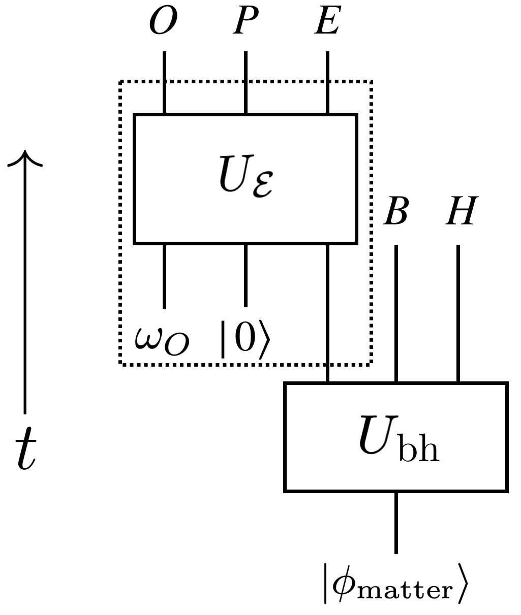
In the case of an “old” black hole , which has already radiated away over half of its initial entropy and has become nearly maximally entangled with , we have . Because the lifetime of an evaporating black hole scales like the power of its initial system size, we may regard the unitary transformation to be “efficient,” meaning that it can be accurately described by a quantum circuit whose size increases only polynomially with . Our key assumption is that the efficient unitary creates a pseudorandom state of (see Section 5). The notion of a pseudorandom quantum state will be further discussed in Section 4.
In the context of the AMPS puzzle, the recently emitted system should be purified by a system behind the horizon. We will explore the idea that this system is actually encoded in , the union of the black hole system and the early radiation system . Let us denote the state prepared by the unitary map as , and consider its expansion
| (1) |
There is a corresponding map defined by
| (2) |
where is the dimension of . If is maximally mixed in the state , then is an isometric map embedding in . We interpret as the encoding map of a quantum error-correcting code, which maps the interior system to the subspace of with which is maximally entangled.
If is any operator acting on , there is a corresponding “logical” operator acting on defined by
| (3) |
This logical operator is not uniquely defined, because equation (3) only specifies its action on the code space, the image of . We may say that is the “mirror operator” of determined by , whose defining property is that and produce the same output when acting on the state .
We wish to investigate whether an agent who interacts with only the radiation system can manipulate the encoded system . For that purpose we introduce an additional system to represent an observer outside the black hole who interacts with . This interaction is modeled by a unitary transformation acting on , possibly followed by a simple measurement performed on ; for example one might measure all the qubits of in a standard basis). The unitary transformation, but not the following measurement, is shown in Figure 1. After the interaction, but before is measured, the joint state of has evolved to
| (4) |
where is the initial state of before and interact.
Our notation for the unitary transformation is motivated by a widely used convention in the theory of quantum channels, in which denotes a quantum noisy channel (a trace-preserving completely positive map), with the letter indicating an “error” acting on the input to the channel. A quantum channel always admits a dilation (also called a purification), a unitary transformation which acts on the input system and an “environment,” after which the environment is discarded. In our context, the noisy channel acting on arises from the action of the observer, and we may regard the observer’s system as the environment in the dilation of . In the following discussion, we will often omit the subscript on , leaving it implicit that acts on the radiation system and observer .
Now we can appeal to a standard result in the theory of quantum error correction. In we regard as a “reference system” which purifies the maximally mixed state of the encoded system . Is there a recovery operator which can be applied to to correct the error induced by this noisy channel? In fact a recovery operator that corrects the error exactly exists if and only if the marginal state of factorizes,
| (5) |
in which case we say the reference system “decouples” from the environment . Heuristically, the error can be corrected if and only if no information about the state of leaks to the environment . There is also an approximate version of this statement Bény and Oreshkov 2010; Flammia et al. 2017. Roughly speaking (we will be more precise in Section 6), recovery with fidelity close to one is possible if and only if and are nearly uncorrelated after and interact.
Now consider the implications of our assumption that the Hawking radiation is pseuodorandom. As stated in Section 1, the marginal state is pseudorandom if cannot be distinguished from a maximally mixed state by any circuit with size polynomial in , apart from an error exponentially small in . We will show in Section 6 that, assuming , if is pseudorandom and is any polynomial-size unitary transformation, then and approximately decouple up to an error exponentially small in . Therefore, apart from an exponentially small error, a computationally bounded observer is unable to inflict an uncorrectable error on the encoded system .
We can make a stronger assertion: It is possible to choose the logical operators acting on the encoded system to be robust ghost operators, which (acting on the code space) nearly commute with any operation applied by the computationally bounded observer . Returning now for simplicity to the setting of exact correctability, we claim that if the error induced by is correctable, then for any operator acting on system , it is possible to choose the corresponding logical operator satisfying equation (3) such that
| (6) |
In this sense, the correctable errors have no effect on the ghost logical algebra. This claim is a special case of a more general statement about operator algebra quantum error correction (OAQEC) Bény et al. 2007a; Bény et al. 2007b. Since we do not expect a black hole to provide an exact error-correcting code, we will need to analyze the case of approximate quantum error correction. Unfortunately, it does not seem straightforward to generalize the results of Bény et al. 2007a; Bény et al. 2007b to the approximate setting. Instead, we present a self-contained construction of exact ghost logical operators in Section 8.1, without making direct use of known results from the theory of OAQEC, and then generalize the construction to the approximate setting in Section 8.2.
We will apply the approximate version of this result to the situation where induces an approximately correctable error, thus inferring that the logical operators acting on the encoded system may be chosen so that they nearly commute with the actions of the computationally bounded observer . We propose that these robust ghost operators are the logical operators acting on the black hole interior, and conclude that the interior is very well protected against the actions of any realistic observer who resides outside the black hole.
The statements about the indistinguishability of from a maximally mixed state, the decoupling of from , the correctability of , and the commuting action of and on the code space, are all approximate relations with exponentially small corrections. Therefore, we need to be mindful of these corrections in constructing our arguments. Fortunately, many relevant features of approximate quantum error-correction have been previously studied, and we make use of results from Bény and Oreshkov 2010; Flammia et al. 2017 in particular.
For the general argument sketched above we have assumed that the observer system satisfies . But it is also instructive to consider a different scenario, in which the observer has access to an auxiliary probe system . We now imagine that the probe , which might have a size comparable to or larger than , is prepared in a simple initial state and then interacts efficiently with . After this interaction between and , the observer (still satisfying ), interacts with , performing an efficient quantum computation that may be chosen adversarially. In this case, too, we can show under the same pseudorandomness assumption as before that the reference system decouples from , and that robust ghost logical operators can be constructed. For example, the probe might cause all of the qubits of to dephase in a preferred basis, but the entanglement between and would still be protected. The modification from the previously considered case is that now will be encoded in rather than , and we conclude that the encoded black hole interior remains inaccessible to any computationally bounded observer who examines the radiation and the probe, as long as the size of the observer’s memory satisfies .
Our conclusion that is difficult to decode or manipulate follows from the pseudorandomness of the Hawking radiation if the observer is computationally bounded and has access only to the radiation system outside the black hole. But we might imagine that an observer who jumps into the black hole has access to the black hole degrees of freedom as well as . We show in Section 9 that an observer who has access to can efficiently manipulate and decode , assuming only that the state was created by an efficient unitary process. In this sense, an interior observer can interact with the interior degrees of freedom, as one might expect. A similar remark applies to the fully evaporated black hole. If the final state after complete evaporation is a highly scrambled pure state of , where , then the maximally mixed state of is purified by a code subspace of . If has constant size, then the code state can be efficiently distilled and deposited in a small quantum memory, assuming only that the map from the infalling matter to the outgoing Hawking radiation is an efficient unitary process.
If an efficient measurement of can detect the correlation between and , then we may expect that an observer acting on is able to interact efficiently with the black hole interior. In Appendix D, we show that, if a product observable has an expectation value in the state that differs significantly from its expectation value in a maximally mixed state of , then there cannot be a complete set of ghost logical operators on commuting with . It follows that, if can be realized efficiently, low-complexity operations acting on the Hawking radiation can send a signal to the interior.
3 Classical pseudorandomness
Our argument that the black hole interior is inaccessible to computationally bounded exterior observers hinges on the hypothesis that the Hawking radiation emitted by an old black hole is pseudorandom. In this section we’ll provide background about the concept of pseudorandomness, which some readers might find helpful.
As discussed in Section 1, we are interested in a black hole that is still macroscopic but has already been evaporating for longer than its Page time Page 1993. The state of the previously emitted radiation system is purified by the black hole system , and by this time is much larger than ; therefore the microscopic state of has far lower rank than a thermal state. It must then be possible, at least in principle, to distinguish from a thermal state. But how, operationally, would an observer outside the black hole who interacts with the radiation be able to tell the difference?
To start with, it will be instructive to consider a simple classical model that captures some of the features of this setup — after we understand how the classical model works we’ll be better prepared to analyze an analogous quantum model. Let’s suppose that the emitted Hawking radiation is a classical bit string of length , which our observer is permitted to read. But this bit string is not chosen deterministically; rather, when the observer reads the radiation he actually samples from a probability distribution governing -bit strings. We’ll say that the state of the black hole is “thermal” if this distribution is the uniformly random distribution , where
| (7) |
But suppose the state of the black hole is described by a distribution that is in principle almost perfectly distinguishable from the uniform distribution. Can this state “fool” the observer, leading him to believe the distribution is uniform even though that is far from the case? See Figure 2.
To be more concrete, let’s suppose the observer is assured that he is sampling from a distribution which is either the uniform distribution , or a different distribution which is uniform on the subset of -bit strings :
| (8) |
where (with ) is the number of strings contained in . The observer samples once from the distribution, receiving , and then executes a classical circuit with as an input, finally producing either the output if he guesses that the distribution is , or the output if he guesses that the distribution is .22 2 The conclusion we reach below would not change much if he were permitted to sample from the distribution a number of times polynomial in .

For large, it is clear that can be chosen so that the observer guesses correctly with a high success probability. Suppose, for example, that he outputs if and he outputs if . It the distribution is actually , this guess is correct with probability . If the distribution is actually , then the guess is correct unless happens to lie in “by accident,” which occurs with probability . Therefore, for fixed and large , the probability of an incorrect guess is exponentially small in .
However, depending on the structure of the set , the circuit that distinguishes and might need to be quite complex, making this strategy impractical if the observer has limited computational power. Suppose, for example, that the observer is unable to perform a computation with more than gates, where grows subexponentially with — that is, where scales sublinearly with . Then we can show that the set can be chosen such that this computationally bounded observer has only an exponentially small chance of distinguishing and ; that is, his probability of guessing the distribution correctly is no better than , where is a positive constant. In that case, we say that the distribution is pseudorandom.
To show that such a pseudorandom distribution exists, we argue in two steps. In the first step, we consider some fixed circuit , and denote by the set of -bit input strings for which outputs 1 (we say that “accepts” the strings in ). If the input is chosen by sampling from , then accepts with probability
| (9) |
while if is chosen by sampling from , then accepts with probability
Now suppose that is chosen randomly from among all subsets of -bit strings with cardinality . We can envision the possible strings as balls, of which the balls accepted by are colored white, and the balls rejected by are colored black, while is a random sample containing of these balls. Suppose that the white balls constitute a fraction of all the balls. Then, for large, we expect that also contains a fraction of white balls which is close to . This intuition can be made precise using Hoeffding’s inequality, from which we derive
| (10) |
where the probability is evaluated for the uniform distribution over all subsets with elements. Now we can choose to have the exponentially small value (for example) to see that, if is sampled uniformly with fixed, the probability that accepts a sample from is exponentially close to the probability that accepts a sample from . We conclude that, not only is it possible to choose the subset such that the fixed circuit can barely distinguish from , but furthermore most choices for with have this property.
We have now completed the first step in our two-step argument. But so far we have only shown that can be chosen such that and are hard to distinguish for one fixed circuit . We wish to make a much stronger claim, that there is a choice for such that and are nearly indistinguishable by any circuit with a number of gates subexponential in .
To prove this stronger claim we proceed with the second step in the argument. For a collection of circuits , what is the probability that , for at least one ? An upper bound on this probability follows from the union bound, which asserts that
| (11) |
where is any set of events. Using equation (10), we conclude that the probability that at least one of the circuits distinguishes from with probability at least is no larger than .
How many possible circuits are there which act on the -bit input and contain computation steps? In each step of the computation, we either input one of the bits of or we execute a gate which is chosen from a set of possible gates, where is a constant. Our claim will hold if each gate in has a constant number of input and output bits, so for simplicity let’s assume that each gate has at most two input bits and generates a single output bit (like a NAND gate for example). Each two-bit gate acts on a pair of bits which are outputs from previous gates; this pair can be chosen in fewer than ways. Therefore, the total number of size- circuits can be bounded as
| (12) |
which implies
| (13) |
Even if we choose an exponentially large circuit size and an exponentially small error , we find that is doubly exponentially small in for and . Hence, if is randomly chosen, it’s extremely likely that the distributions and are indistinguishable by circuits of size , up to an exponentially small error.
To summarize, we’ve shown that the set can be chosen so that the probability distribution has these properties:
- 1.
Its entropy per bit is a positive constant less than 1.
- 2.
It is statistically distinguishable from with an exponentially small failure probability.
- 3.
If , any circuit using at most gates almost always fails to distinguish and .
If is macroscopic, the task of distinguishing from can be absurdly difficult, even if the entropy density is quite small. Suppose, for example, that is comparable to Avogadro’s number, and . Choosing we conclude that a circuit with gates can distinguish from with a success probability no larger than . Even if we could perform one gate per unit of Planck time and Planck volume, an unimaginably large spacetime region would be required to execute so large a circuit.
The existence of pseudorandom distributions was first suggested by Yao Yao 1982, and the construction we have described was discussed by Goldreich and Krawcyzk Goldreich and Krawczyk 1990. In our analysis we assumed that the observer executes a deterministic circuit, but it turns out that giving the observer access to a random number generator does not make his task any easier Goldreich and Krawczyk 1990.
Up until now, we assumed that the observer performs a computation whose output is a single bit. But what if he obtains a -bit output instead? Can we choose the set so that for all circuits of bounded size the probability distribution governing the output bits is very similar for input strings drawn from and ? Our previous reasoning does not have to be modified much to handle this case. Now for the fixed circuit , we denote by the set of -bit input strings for which outputs the -bit string , and we denote by , the probability that outputs when receiving as input a sample from , respectively. Now we envision the -bit input strings as balls which can be colored in possible ways, corresponding to the possible values of the output . Applying the previous argument to each color, we find that when is chosen at random from among all subsets with cardinality ,
| (14) |
for each output . From the union bound, the probability that exceeds for at least one value of is bounded above by , which also provides an upper bound on the probability that the total variation distance between and exceeds . Therefore the total variation distance will be no larger than with high probability as long as is large, which means can be exponentially small in provided . We conclude that the pseudorandom input distribution and the uniformly random input distribution will yield exponentially close output distributions as long as the observer’s output register is small compared to the entropy of .
The preceding argument shows that, indeed, there are probability distributions which are computationally indistinguishable from the uniformly random distribution. But can we make such a distribution efficiently? It turns out that our argument for the computational hardness of distinguishing a pseudorandom distribution from a uniformly random distribution can be used to show that such distributions are typically hard to produce with polynomial-sized circuits.33 3 We thank Adam Bouland for emphasizing this point. However, there are distributions that can be created using polynomial-sized circuits which, under reasonable complexity-theoretic assumptions, are difficult to differentiate from the uniformly random distribution, for any polynomial-sized circuit. Such distributions can be generated by pseudorandom generators Arora and Barak 2009. We will give a more complete description of such constructions for the quantum case in Section 4.
Efficient sampling from a (classical) pseudorandom distribution is analogous to the formation and partial evaporation of a black hole. Pseudorandom number generators consult a random “key” which is hidden from the adversary, and then compute a function which depends on the key. This function is chosen so that an output drawn from the resulting family of outputs indexed by the key is computationally indistinguishable from the output of a truly random function. In the case of the partially evaporated black hole, the key becomes a black hole microstate, and the key-dependent function evaluation becomes the chaotic unitary evolution of the evaporating black hole. An adversary samples the Hawking radiation, and attempts to determine whether the sample is drawn from a thermal distribution or not.
To properly discuss the evaporating black hole, we will need to consider the quantum version of pseudorandomness, to which we turn in the next two sections. But our simplified classical model of “Hawking radiation” is instructive. It teaches us that the (classical) adversary can interact with the (classical) radiation for a subexponential time (or even for the exponential time if is sufficiently small), without ever suspecting that the radiation is far from uniformly random. On the other hand, that conclusion may no longer apply if the adversary collects bits of information where is sufficiently large (. Both of these features will pertain to the quantum version of our story.
4 Quantum pseudorandomness
Now consider the quantum version of the task described in the Section 3. Our observer receives a quantum state , and is challenged to guess whether is maximally mixed or not. For that purpose, he performs a quantum computation with as input, and he outputs a single bit: 0 if he guesses is maximally mixed and 1 otherwise.
Following our analysis of the classical case, let’s first suppose that the observer executes a particular fixed quantum circuit. That means the observer measures a particular Hermitian observable with unit operator norm. Suppose we try to fool the observer by providing as input a pure state . How well can the observable distinguish this pure state from the maximally mixed state?
Suppose that is chosen uniformly at random from among all -qubit pure states. Then Levy’s lemma Hayden et al. 2006 says that
| (15) |
for some constant , where the probability is evaluated with respect to the invariant Haar measure on the -qubit Hilbert space. This means that, for large, the pure state can be chosen so that and the maximally mixed state are exponentially difficult to distinguish using the observable . Furthermore, most pure states have this property. Even a pure quantum state can pretend to be maximally mixed, and the observer will not know the difference!44 4 If two identical copies of are available, then it is easy to distinguish the pure state from the maximally mixed state by conducting a swap test. Here we assumed that only a single copy is available.
As in the classical case we can strengthen this claim: The state can be chosen so that is hard to distinguish from the maximally mixed state not just for one fixed quantum circuit, but for any quantum circuit of reasonable size. To carry out this step of the argument, we’ll need an upper bound on the number of quantum circuits of specified size; here we confront the subtlety that quantum circuits, unlike classical ones, form a continuum, but this wrinkle poses no serious obstacle to completing the argument. If we settle for specifying the unitary transformation realized by a circuit with gates to constant accuracy, it suffices to specify each gate to bits of precision. Therefore, as in the classical case, the complete circuit can be specified by bits. It follows that, if is subexponential in , then the number of circuits with size is the exponential of a function which is subexponential in . In contrast, the right-hand side of equation (15) is the exponential of an exponential function of . Using the union bound, we conclude that if the pure state is chosen uniformly at random, it will, with high probability, be hard to distinguish from the maximally mixed state using any circuit of size subexponential in .
On the other hand, if we were not concerned about the complexity of the observer’s task then it would be easy to distinguish from the maximally mixed state. The observer could perform a projective measurement with the two outcomes , guessing that the input state is if he obtains the outcome , and guessing that the input state is maximally mixed if he obtains the outcome . This strategy always succeeds if the input is , and fails with the exponentially small probability if the input is maximally mixed. The trouble is that, for a typical pure state , this measurement is far too complex to carry out in practice.
A typical pure quantum state is somewhat analogous to the distribution we described in Section 3. In both cases, it is hard for an observer who is limited to performing polynomial-size computations to tell that the state is not uniformly random, even though an observer with unlimited computational power can tell the difference. Furthermore, both examples are subject to the same criticism — it is computationally hard to sample uniformly from Haar measure (that is, to prepare a “typical” pure state), just as it is computationally hard in the classical setting to sample from the the distribution . In the quantum setting, as for the classical setting, we may ask a more nuanced question: Can quantum states be prepared efficiently which are hard to distinguish from maximally mixed states? This more nuanced question is the relevant one as we contemplate the properties of the radiation emitted by a partially evaporated black hole, because the formation and subsequent complete evaporation of a black hole can occur in a time that scales like , where is the initial black hole entropy. Hence, the preparation of the Hawking radiation can be simulated accurately by an efficient quantum circuit.
The answer is yes (under a reasonable assumption), as was shown recent by Ji, Liu, and Song Ji et al. 2018; pseudorandom quantum states can be prepared efficiently. The assumption we need is the the existence of a family of quantum-secure pseudorandom functions . This means that each can be efficiently computed, but it is difficult to distinguish a randomly sampled member of from a truly random function with any efficient quantum algorithm. The set is called the key space of the function family. The existence of such pseudorandom functions follows from the existence of quantum-secure one-way functions, an assumption which is standard in cryptography.
The key idea is that we can construct a pseudorandom quantum state as a superposition of computational basis states, where all basis states appear with equal weight except for a phase, and the phases appear to be random to a computationally bounded observer. Specifically, we consider a family of states
| (16) |
where , , , and is a family of quantum-secure pseudorandom functions. We can show that a uniform mixture of the states is computationally indistinguishable from the maximally mixed state.55 5 In fact, we can simplify the construction. It was shown in Brakerski and Shmueli 2019 that the same family of states is still pseudorandom if we replace the root of unity by .
We may argue as follows. First we consider the family of all functions indexed by key space , and the corresponding family of pure states
| (17) |
The first thing to note is that is information-theoretically indistinguishable from Haar-random; we state this fact for the reader’s convenience in Lemma 4.1.
Lemma 4.1 (Ji et al. 2018, Lemma 1).
Let be the family of states defined in equation (17). Then, for polynomial in , the state ensemble is statistically indistinguishable from the ensemble where is Haar-random, up to a negligible error.
Furthermore, the ensemble cannot be efficiently distinguished from the ensemble . If it could be, then we could leverage this fact to efficiently distinguish from a family of random functions Ji et al. 2018, contradicting our assumption that is a quantum-secure pseudorandom function family. It now follows that the ensemble cannot be efficiently distinguished from a maximally mixed state.
So far we have shown that a uniform mixture of the states is pseudorandom; it remains to show that this mixture can be prepared efficiently. We start with a product of qubits, each in the state , and apply a Hadamard gate to each qubit to obtain the state
| (18) |
Next, we apply the quantum Fourier transform (which has complexity polynomial in ) to another -qubit register that is initialized in the state , obtaining
| (19) |
Now, we compute and subtract modulo from the register. This computation can be done efficiently because by assumption the is an efficiently computable function; the resulting state is
| (20) |
After shifting the summation index , we have, up to a global phase,
| (21) |
where . After the key is discarded, the marginal state over the first register is the uniform mixture of . Thus, we have prepared this mixture efficiently.
The definition of a pseudorandom quantum state in reference Ji et al. 2018 is really overkill for our purposes. Those authors are concerned with cryptographic applications, and therefore consider a definition (as stated in Lemma 4.1) where, for each value of the key, identical copies of are available where is polynomial in . We will not encounter such scenarios in this paper. Therefore, we may instead adopt a simplified definition of pseudorandomness which is more suitable for the application to black hole physics. In Definition 6.1 below, the size of the remaining black hole parametrizes how difficult it is to distinguish radiation emitted from the partially evaporated black hole from the maximally mixed state. In this sense, the remaining black hole serves as the key space of the pseudorandom radiation state. Even if is less than half of the initial black hole entropy, this task remains difficult so long as the remaining black hole is macroscopic. Our hypothesis that the Hawking radiation is pseudorandom provides a way to formalize the idea that the Hawking radiation is effectively thermal even when the state of has relatively low rank because .
5 Is Hawking radiation pseudorandom?
We have now seen, in both the classical and quantum settings, that pseudorandom states exist. Though in principle these states are almost perfectly distinguishable from maximally mixed states, in practice no observer with reasonable computational power can tell the difference. Moreover, under standard cryptographic assumptions, there exist constructions of such states which can be efficiently prepared. But up to this point we have not addressed whether pseudorandom quantum states can be efficiently prepared in plausible physical processes like the evaporation of a black hole.
In the case of a black hole which forms from gravitational collapse and then completely evaporates, the resulting state of the emitted Hawking radiation, though highly scrambled, would not be pseudorandom. We take it for granted that the time evolution of the quantum state can be accurately approximated by a quantum circuit, which has size polynomial in the initial black hole entropy because the evaporation process takes a time . We may consider a toy model of this process, in which the initial state of the collapsing matter is a product state of qubits , and the final state after complete evaporation is , where is a unitary transformation constructed as a polynomial-size circuit. In this case, an observer could just execute this circuit in reverse, hence applying to , and then measure the qubits in the standard basis, thus easily distinguishing from the maximally mixed state. We see that, if is a state that can be prepared by a polynomial-size quantum circuit, yet is hard to distinguish from maximally mixed by polynomial-size circuits, then cannot be pure.
Instead, we consider a partially evaporated black hole as in Figure 3. We imagine that the -qubit state is prepared by applying a polynomial-size unitary circuit to the initial state of , where is a -qubit system, and then discarding . In our toy model, is the Hawking radiation that has been emitted so far, and is the remaining black hole. (Recall that is a small portion of the emitted Hawking radiation whose properties we will investigate later; for the purpose of the present discussion we are only interested in the state of , the full radiation system.) If our observer had access to as well as , he could easily tell that the state is not maximally mixed, but what if is inaccessible?

We are particularly interested in the case where , so that fails to have full rank, and must therefore be information-theoretically distinguishable from the maximally mixed state; this situation resembles the classical model discussed in Section 3, where the entropy of the distribution is substantial but not maximal. Could the state of the Hawking radiation, which is prepared by unitary evolution of for a time which is polynomial in , be pseudorandom?
This is a question about quantum gravity, and we don’t know the answer for sure, but we can make a reasonable guess. We have already seen in Section 4 that quantum circuits exist that efficiently prepare pseudorandom quantum states. Since black holes are believed to be particularly potent scramblers of quantum information, it is natural to conjecture that the internal dynamics of a black hole can produce pseudorandom states as well. Indeed, we may expect similar behavior for the radiation emitted by other strongly chaotic quantum systems aside from black holes. Only for the case of black holes, though, where we face the daunting firewall puzzle, will our constructions of robust logical operators acting on seem to have a natural interpretation.
To better understand why the state of might be hard to distinguish from a maximally mixed state, we may suppose, for example, that is maximally mixed so that the pure state of has the form
| (22) |
where the states are orthonormal. The marginal state of is then
| (23) |
Suppose the observer receives a state which is either or the maximally mixed state . A natural test is as follows: The observer augments with the maximally mixed state of (which is easy to prepare), and then measures the projection onto . This can be done efficiently by applying and then measuring in the standard basis. If the input state is , the projection onto succeeds with probability , while if the input state is the success probability is
| (24) |
Thus this test distinguishes and , but only with a probability that is exponentially small in .
To conduct a better test we would somehow need to exploit the structure of the ensemble . But if as we expect black holes are especially effective information scramblers, it is reasonable to suppose that the ensemble lacks any special properties that can be exploited by an observer who is limited to performing a polynomial-time quantum computation. If so, the Hawking radiation is pseudorandom, and the test we have described may be nearly optimal.
In the example above we have assumed that the radiation has infinite temperature. The actual behavior of a black hole evaporating in asymptotically flat spactime is more complicated — the temperature is actually finite, and in fact becomes hotter and hotter as the evaporation proceeds. Conceptually, though, the situation is similar to the idealized case of an black hole evaporating at infinite temperature. At early times, when , we expect the radiation emitted at a specified time to be information-theoretically indistinguishable from precisely thermal radiation at the same temperature. At late times, when , the global state of the radiation is distinguishable in principle from a thermal state (with temperature varying according to the time of emission), but we assume that telling the difference is computationally hard because the radiation is highly scrambled.
We also note that the constructions in Ji et al. 2018 reinforce earlier observations concerning the computational hardness of decoding the Hawking radiation Harlow and Hayden 2013; Aaronson 2016. These authors considered the quantum state of an old black hole, and analyzed the task of extracting from the early radiation the subsystem which is entangled with the recently emitted Hawking mode . This task would be easy for an observer who has access to both and , but one can argue that there are efficiently preparable states of for which this decoding task cannot be achieved by an observer who performs a polynomial-size quantum computation on alone. Here, too, the hardness of decoding cannot be proven from first principles, but it follows from plausible complexity assumptions which are standard in “post-quantum” cryptography Harlow and Hayden 2013; Aaronson 2016. Again, the existence of states that are hard to decode does not guarantee that a black hole creates such states, but we take it on faith that if efficient preparation of such states is possible, then a black hole will be up to the job.
To summarize, on the basis of these (admittedly speculative) considerations, we propose that for the quantum state of an old black hole, the state of the Hawking radiation is pseudorandom. If , then the rank of is not maximal, so that is distinguishable from a thermal state. In fact, an observer with access to as well as could efficiently check that is not thermal. Furthermore, an observer without access to could check that is not thermal by performing a quantum computation of exponential size on alone. But an observer outside the black hole, who performs a polynomial-size quantum computation on without access to , will be able to distinguish from a thermal state with a success probability that is at best exponentially small in . Our analysis of the robustness of the encoded black hole interior in the remainder of this paper will rest on this assumption.
This discussion highlights the importance of distinguishing the von Neumann entropy of the Hawking radiation from its thermodynamic entropy. After the Page time, the Von Neumann entropy of becomes far smaller than the von Neumann entropy of a perfectly thermal state, so one could in principle verify that the Hawking radiation is not perfectly thermal by measuring its von Neumann entropy. The existence of pseudorandom quantum states then implies that measuring the von Neumann entropy with a small error requires an operation of superpolynomial complexity Gheorghiu and Hoban 2020. One could imagine trying to measure the entropy of the radiation by, for example, withdrawing its thermal energy to operate a heat engine. If the radiation is pseudorandom, though, the radiation would be indistinguishable from thermal radiation in any efficient process, despite its low von Neumann entropy.
Recalling the construction of the pseudorandom state recounted in Section 4, we note Cleve and Watrous 2000 that the quantum Fourier transform can be executed with circuit depth , and that under plausible cryptographic assumptions the function can be computed in depth polylog Ji et al. 2018. Thus a pseudorandom state can be prepared in polylog time. Plausibly, the state preparation can be achieved in a time comparable to the scrambling time of a black hole, as one might naively expect.
6 Pseudorandomness and decoupling
In this section, we formalize our hypothesis that Hawking radiation is pseudorandom, and explore its implications regarding the firewall paradox Almheiri et al. 2013a. Our analysis can be viewed as a refinement of the Harlow-Hayden argument Harlow and Hayden 2013; Aaronson 2016.
As formulated in Almheiri et al. 2013a and summarized in Section 1, the firewall paradox highlights a conflict between the unitarity of black hole evaporation and the monogamy of entanglement. A possible resolution is that the interior mode that purifies a recently emitted Hawking mode may actually be encoded in the radiation. On the face of it, this resolution flagrantly violates locality, and one wonders whether this violation of locality can be detected by an agent who first interacts with the radiation and then falls through the event horizon to visit the interior. We will argue that, provided the Hawking radiation is pseudorandom and the size of the observer is small compared to the black hole, the nonlocality is undetectable in practice because it would take an exponentially long time for the observer to distill the encoded interior mode before falling into the black hole.
We will first present a sketch of the argument in a simplified setting where the radiation interacts with a single observer who is significantly smaller than the remaining black hole. Later on we will extend the argument to the case where the observer has access to a large probe outside the horizon, whose size may be comparable to or even larger than the remaining black hole.
Recall our conventions: Let denote the observer, the remaining black hole, the late outgoing mode, the early radiation, and the external probe. We will also refer to the joint system as the exterior radiation. All subsystems can be decomposed in terms of qubits, and our statements about computational complexity concern the number of steps in a computation executed by a universal quantum computer. Below and throughout the remainder of the paper, given an operator , we will use to denote the trace norm, to denote the Frobenius norm, and to denote the operator norm.
First, we define what it means for the external radiation of the black hole to be pseudorandom.
Definition 6.1.
Let be the state of the black hole and the radiation. Let be the maximally mixed state of , and let . We say that the state is pseudorandom on the radiation , if there exists some such that
| (25) |
for any two-outcome measurement with quantum complexity polynomial in , the size of the remaining black hole.
This definition captures the notion that no feasible measurement can tell the difference between and the maximally mixed state. A few remarks will help to clarify the definition. (1) When we say a measurement of has polynomial quantum complexity, we mean it can be performed by executing a quantum circuit of polynomial size acting on , followed by a qubit measurement in the standard computational basis. Use of ancilla systems is also permitted in the measurement process, provided the ancilla is initialized in a product state. (2) Of particular interest is the value of the constant that makes the bound in equation (25) tight for asymptotically large black holes. But because black holes are such effective information scramblers, we would expect a comparable value of to apply also for black holes of moderate size. There is no obvious small parameter in the problem that would lead us to expect to be small compared to 1. (3) This definition is appropriate for the case where the Hawking radiation has infinite temperature. As we remarked in Section 5, we expect the realistic case of finite-temperature radiation to be conceptually similar, and for similar conclusions to apply in that case. But we will stick with the infinite-temperature case for the rest of the paper to simplify our analysis.66 6 In the finite temperature case, the entanglement between and the rest of the system is no longer maximal. This causes an extra complication when we use the quantum error-correction technology in Section 7, because the encoding map from to defined by the state need not be exponentially close to an isometry. Instead we may replace by the approximate isometry , which slightly modifies the error bounds derived in Section 7 and 8. Similar techniques have been used in Papadodimas and Raju 2013; Papadodimas and Raju 2016; Harlow 2014.
Let us now deduce a consequence of Definition 6.1. We introduce an observer subsystem initialized in a state , and an ancilla subsystem initialized in the product state . The main result of this section is the following: Suppose that is pseudorandom, and let be any state of obtained by applying a unitary of polynomial complexity to . Then the correlation between the observer and the early radiation is exponentially small in for any such state; i.e.,
| (26) |
where we have now assumed that is a single qubit. We will call (26) the decoupling bound, because it states that the observer nearly decouples from the exterior radiation mode , and therefore gains negligible information about the interior mode which is entangled with . In Section 8 we leverage (26) to show that the interior mode can be regarded as an encoded subsystem of which is protected against all “low-complexity” errors, where “low-complexity” is shorthand for polynomial complexity.
Prior work Harlow and Hayden 2013; Aaronson 2016 has suggested that the decoupling bound holds when the size of the remaining black hole is an fraction of the initial black hole entropy . However, our conclusion goes further. Even if the majority of the initial black hole has evaporated, so that , the observer and the late radiation remain decoupled as long as the remaining black hole is macroscopic and the observer’s system obeys .
To derive the decoupling bound, we apply the pseudorandomness assumption to the setup described in Figure 1. The unitary is applied to the radiation, probe, and the observer. Because the evaporation time of the black hole is polynomial in its size, and is applied before the evaporation is complete, we may assume that is applied in a polynomial time and therefore has polynomial complexity. We also assume that the initial state of the observer is of low complexity, although this assumption is not crucial; we may take the state to be arbitrary, at the cost of a slightly weaker decoupling bound.
In order to bound the correlation between and , we consider a complete set of operators acting on . A convenient choice is the set of Pauli operators acting on . By a Pauli operator acting on qubits we mean a tensor product of Pauli matrices; there are such operators (where ) whose phases can be chosen so that each for has eigenvalues , and the are orthogonal in the Froebenius norm: . Here is the number of qubits in . Because measurement of is a low-complexity two-outcome measurement, it follows from the assumption that is pseudorandom that
| (27) |
for any Pauli operator , where is the state that results when the state measured by the observer is replaced by the maximally mixed state; see Figure 4.
To understand why equation (27) follows from pseudorandomness, note that we are modeling a measurement of by the observer as a low-complexity unitary interaction between and , followed by a simple measurement of the register. Strictly speaking, then, we should allow the Pauli operator to act only on , not on . In effect, we are assuming that the observer’s quantum memory contains qubits rather than qubits, so that measuring a Pauli operator acting on is permitted. In our formulation of the pseudorandomness assumption, there is no restriction on the size of the observer’s memory, only on the complexity of his operation. Therefore, assuming that the state of is pseudorandom, the observer’s measurement will not distinguish from even if the observer is permitted to measure as well as .
Using the completeness and orthogonality of the Pauli operators, we can bound the Frobenius distance between the two states as
| (28) | ||||
| (29) |
Because there are Pauli operators, the right hand side is bounded by . The trace distance is bounded by the Frobenius norm as
| (30) |
for any operator . Therefore we have
| (31) |
because the rank of can be no larger than . From (31), one finds that
| (32) | ||||
The first line is the triangle inequality. From the first line to the second line, we used (31). From the second line to the third line we used the fact that is a product state over and . From the third line to the fourth line, we used the fact that
| (33) | ||||
where the first line of (33) follows from the triangle inequality, and the second from the property that tracing out a subsystem cannot increase the trace distance. To reach the last line of (32), we again used the property that tracing out a subsystem cannot increase the trace distance. Finally, in the case where is a single qubit, so that , (32) becomes the decoupling bound (26). More generally, decoupling is satisfied whenever .

Because two states close in trace distance cannot be distinguished well by any measurement, the decoupling bound implies that the state cannot be distinguished from the state assuming that . We thus conclude that any subsystem small compared to the remaining black hole , even after interacting with the early radiation , cannot be correlated with ; see Figure 4. In particular, an observer outside the black hole who interacts with for a polynomially bounded time remains decoupled from , assuming that the Hawking radiation is pseudorandom.
This conclusion about the hardness of decoding follows from the pseudorandomness assumption for any computationally bounded observer who can access only system . However, the decoding becomes easy if the observer has access to both and , as long as the state has polynomial complexity. For this case, we will describe an explicit decoding protocol in Section 9.
7 Black hole as a quantum error-correcting code
In this section, we recast the findings in Section 6 in the language of quantum error correction. The quantum error correction point of view will prove to be useful in understanding more subtle thought experiments studied in Section 8. We will see that an old black hole, together with its previously emitted Hawking radiation, is a quantum error-correcting code with exotic properties that have not been noted in previous discussions of holographic quantum error-correcting codes Almheiri et al. 2015; Pastawski et al. 2015. These properties hold if the Hawking radiation is pseudorandom. That a black hole can be viewed as a quantum error-correcting code is not new Pastawski et al. 2015; Hayden and Penington 2019; Verlinde and Verlinde 2013; Yoshida 2019a. What’s new is that a black hole can protect quantum information against seemingly pernicious errors; we refer to these as “low-complexity errors,” meaning errors inflicted by a malicious agent who performs a quantum computation on the Hawking radiation with complexity scaling polynomially in the size of the remaining black hole.
To explain this claim, it is useful to view the state of the black hole and the radiation as an encoding map from the interior mode into . That is, defines an isometric embedding of into . Recall that denotes the early radiation, denotes the remaining black hole, and denotes a late outgoing mode. For simplicity, we assume that is a single qubit, but the following results remain essentially unchanged for of any constant size (small compared to ). The encoded system describes the mode in the black hole interior that is entangled with .
We can define an (approximate) isometric embedding of a single qubit into the subspace by
| (34) |
where denotes an EPR pair on ; see Figure 5. While itself is not precisely an isometric embedding, it is exponentially close to one under the assumption that is pseudorandom on the exterior system , as specified in Definition 6.1. In Appendix A, we show that there exists an isometric embedding such that
| (35) |
where denotes the operator norm. The isometry then defines a code subspace that encodes . For macroscopic observers (i.e., ), the error in (35) is negligible compared to the error in the decoupling bound (26). Although the norm in equation (35) is the operator norm rather than the trace norm, that distinction need not concern us if is sufficiently small compared to . Therefore we can ignore any differences between and and use them interchangeably.

We will now show that the isometry defined above embeds into as a code subspace for which any low-complexity noise model acting on is (approximately) correctable. By low-complexity error, we mean that the unitary process in Figure 6 has complexity at most polynomial in . Here the external observer plays the role of the “environment” for the noise process acting on and the probe .
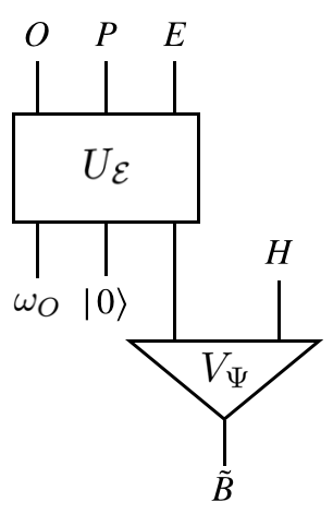
The error model depicted in Figure 6 is rather exotic compared to error models that are typically considered in discussions of quantum gravity and fault-tolerant quantum computing. For example, one widely studied error model is the “erasure model,” wherein each qubit may be removed with some probability, and we know which qubits are removed. The performance of quantum codes against erasure errors arises, in particular, in studies of the holographic AdS/CFT dictionary Almheiri et al. 2015; Pastawski et al. 2015; if a logical bulk operator can be “reconstucted” on a portion of the boundary, that means that erasure of the complementary portion of the boundary is correctable for that logical operator. By the no-cloning theorem, no code can tolerate erasure of more than 50% of the qubits in the code block. In contrast, in our setup, erasure is correctable even if most of the qubits are removed. The catch is that the erased qubits must lie in ; removal of qubits in is not allowed.
In studies of fault-tolerant quantum computing, the noise afflicting the physical qubits is usually assumed to be weak and weakly correlated. In a Hamiltonian formulation of the noise model, this means that each qubit in the computer is weakly coupled to a shared environment Preskill 2013. In contrast, for the noise model described by , the noise may act strongly on all the qubits in ; the only restriction is that the noise has quantum complexity scaling polynomially with . Furthermore, how the noise acts depends on the initial state of the observer , which may be chosen adversarially. Again, what makes successful error correction possible is that the subsystem is assumed to be noiseless, an assumption that would be unrealistic for typical quantum computing hardware.
Codes that can protect against this malicious typle of noise are central to our proposed resolution of the firewall paradox. An old black hole provides such a code if its previously emitted radiation is pseudorandom. The code corrects errors successfully if the noise acting on has low complexity and the remaining black hole is noiseless, provided that the observer is small compared to .
7.1 Correcting low-complexity errors
For simplicity, we will first consider a scenario without the probe shown in Figure 6. We will see that the error applied to the radiation system is (approximately) correctable. In Section 7.2 we will explain how our conclusion changes when the probe is included.
A central result in the theory of quantum error correction is the information-disturbance relation, which states that a code can protect quantum information from noise if and only if the “environment” of the noise channel learns nothing about the logical information. More precisely, there is a physical process , the recovery process, which reverses the error:
| (36) |
where is the identity operation, if and only if the “reference system” that purifies the quantum error-correcting code decouples from the environment . In Figure 6 (neglecting the probe ), the environment of the noise channel acting on is the observer , and is the reference system that purifies the encoded interior mode . Therefore the necessary and sufficient condition for (approximate) correctability is the (approximate) decoupling of and ,
| (37) |
where is the reduced density operator for . Here the approximation errors of equation (36) and equation (37) are related to each other by a constant factor. Therefore, using the decoupling bound (26), we can conclude that there exists a recovery process that reverses up to an error exponentially small in , as long as and assuming that the Hawking radiation is pseudorandom.
Various formal statements that imply the existence of in equation (36) are known; for the reader’s convenience, we reproduce some of these results below. First, let us properly define what it means for a channel to be approximately correctable with respect to some code subspace — a more comprehensive discussion can be found in Bény and Oreshkov 2010. Let denote the set of states on a Hilbert space . Suppose that we are given channels . Fixing a state , we define the entanglement fidelity between and with respect to to be
| (38) |
where is a purification of , and where
| (39) |
is the usual fidelity between states and . To quantify the closeness of two channels, we use the worst-case entanglement fidelity to define the Bures distance, given by
| (40) |
we sometimes define a more restricted notion of the Bures distance, where we maximize over states in some specified subspace. In discussions of error correction, we say that a noise channel is -correctable with respect to a code subspace if there exists a recovery channel such that
| (41) |
where the maximization in the Bures metric is over all code states with support on .
The Bures metric is bounded above and below by the trace norm as
| (42) |
The norm in the middle is essentially the diamond-norm distance between the channels and Nielsen and Chuang 2011, except that for the purpose of characterizing error correction the maximization is over code states only. Applying this inequality and tracing out the purifying system, the -correctability of a channel implies that we have
| (43) |
where again the maximization is over code states.
As mentioned previously, an important result characterizing approximate correctability is the information-disturbance trade-off, which we now state quantitatively. Let be a noise channel acting on a system , and let be an isometry which purifies ; i.e.,
| (44) |
Hence is the environment of the channel; we have resisted the temptation to denote the environment by to avoid confusion with our convention that denotes a subsystem of the Hawking radiation. Then the complementary channel is defined by
| (45) |
A special case of interest is the identity channel . Taking the environment to be -dimensional, the complementary channel to the identity channel is simply the (partial) trace
| (46) |
Then the information-disturbance trade-off states the following:
Theorem 7.1 (Bény and Oreshkov 2010, Theorem 1).
Let be a code subspace. Let be an error channel. Then
| (47) |
where the infimums are taken over all channels , and .
Note that a channel is just state preparation on the channel environment , i.e., every such channel is uniquely identified with a state such that
| (48) |
so we can equivalently write
| (49) |
Now let’s see what equation (47) tells us in the context of the black hole error-correcting code defined by the (approximate) isometry . Let be a logical state and let be a purification. The isometry then embeds as a (purified) code state :
| (50) |
Let be an arbitrary channel acting on such that some purification of has low-complexity (see the set-up described in Figure 1). Let
| (51) |
denote the overall post-evolution state. To apply Theorem 7.1, let us consider the error channel . Then the environment of the channel is the observer subsystem , and the complementary channel maps to . From (51), the state obtained from after the application of is precisely given by
| (52) |
Since was a state obtained through acting on the black hole code state with a low-complexity unitary, it follows by the pseudorandom hypothesis that the decoupling bound (26) holds. Therefore we have
| (53) |
Finally, since is supported away from , we have , and so
| (54) |
This holds for all code states, so (54), together with the first inequality in (42), implies that we have
| (55) |
Therefore, the channel is approximately correctable by Theorem 7.1. We state this as a Lemma.
Lemma 7.2.
Let be the approximate isometric embedding defined by the state . Let be an error channel on with purification . Suppose that the decoupling bound (26) holds. Then is -correctable for , where
| (56) |
if is a single qubit. For general , we have
| (57) |
Note that the recovery operator acts on rather than . The same will be true for the ghost logical operators we construct in Section 8.
7.2 Including the probe
We would now like to consider a modified scenario in which both the observer and a probe interact with the Hawking radiation system , as indicated in Figure 1. We cannot simply absorb into , because we will continue to insist that is small compared to , while we wish to allow to be comparable to in size, or even larger. In this modified scenario, the unitary purification of the noise model acts on rather than . This change does not alter the conclusion that and decouple if has low complexity. Therefore, just as before, there is a recovery map that reverses the effect of the noise on the encoded state. What changes is that now the recovery map acts on rather than .
We emphasize that if the probe is sufficiently large, then need not decouple from , even if has low complexity. To understand why not, suppose has the same size as the system and that the channel swaps and . Before this swap, is entangled with the code space embedded in ; therefore after the swap (a low-complexity operation), is entangled with . More realistically, we might imagine that is a cloud of dust surrounding the black hole, and that . After the dust interacts with the Hawking radiation, the encoding of will be modified, so that is entangled with a code subspace of rather than a subspace of Bousso 2014.
However, any subsystem of which is small compared to will decouple from , as long as has low complexity, and assuming that the Hawking radiation is pseudorandom. The only way to distill the encoded state into a small subsystem is to perform a high complexity operation. Hence, if only low-complexity operations are allowed, we need not worry about a scenario in which the encoded version of outside the horizon is decoded into a small system, and then falls into the black hole to meet its twin in the interior. This is essentially the observation of Harlow and Hayden Harlow and Hayden 2013, later extended by Aaronson Aaronson 2016. Our analysis goes further by clarifying that the encoded state is hard to distill even when the remaining black hole is much smaller than , as long as is macroscopic and assuming that the Hawking radiation is pseudorandom.
One might wonder whether the encoded mode can be easily extracted if the probe system is prepared in a carefully chosen state Oppenheim and Unruh 2014. Our conclusion is that any such initial state of would need to have exponential complexity, an unlikely property for the dust surrounding an evaporating black hole. One might also ask what happens if all the qubits in the early radiation system are measured in the standard basis by the observer. Surely this would disrupt the encoded interior of the black hole. But in our model the number of radiation qubits that can be measured is limited by the size of the observer’s memory, and the interior will stay well protected as long as is much smaller than .
It is also instructive to view the system in a different way. Up to now we have regarded as a potentially malicious agent who attempts to damage the encoded interior of the black hole by acting on its exterior. More prosaically, we can think of as an abstract purifying space which is introduced for convenience so that we can describe the noise channel using its purification, the unitary transformation . From that point of view, limiting the size of the “observer” is just a convenient way of restricting the form of the quantum channel . Specifically, the rank of the marginal density operator after is applied is called the Kraus rank (or simply the rank) of the channel . This rank can be no larger than the dimension of system , namely , which we have assumed to be small compared to the dimension of the Hilbert space of black hole microstates. Thus our conclusion can be restated: If the Hawking radiation is pseudorandom and is macroscopic, then the quantum error-correcting code protects the encoded version of against any noise channel acting on that has both low complexity and low rank.
An advantage of this viewpoint is that one might otherwise be misled into interpreting as the physical size of an actual observer. More accurately, it can be regarded as the effective size of the quantum memory of a physical object. This distinction is significant. For an object of specified mass, the largest possible quantum memory is achieved by a black hole of that mass, but the memory size of a quantum computer typically falls far short of that optimal value, because most of its mass is locked into the rest mass of atomic nuclei and unavailable for information processing purposes. Furthermore, the mass per unit volume of a typical quantum computer is far smaller than a black hole’s. Therefore it is reasonable to expect that the effective Hilbert space dimension of system (and hence the Kraus rank of the channel ) is far smaller than the Hilbert space dimension of a black hole with the same circumference as system .
Up until now we have mostly focused on the hardness of decoding the black hole interior mode by acting on the Hawking radiation outside the black hole, concluding that distilling the encoded system to a small quantum memory is computationally hard if the remaining black hole is macroscopic. In section 8 we will turn to a more subtle question: Can a low-complexity operation acting on the Hawking radiation system create an excitation near the black hole horizon that could be detected by an infalling observer who falls into the black hole? Here too we will argue that the answer is no. This is a nontrivial extension beyond what we have found so far — on the face of it, perturbing a quantum state is a far easier task than depositing the state in a compact quantum memory.
Bousso emphasized that if the interior mode is encoded in , and if effective quantum field theory on curved spacetime is a good approximation in regions of low curvature, then the vacuum near the black hole horizon would need to be “frozen” Bousso 2014. That is, neither a small agent acting on nor a large probe interacting with could disrupt the entanglement of with and hence create an excitation localized near the horizon. We agree with this conclusion, provided that and that the interactions of with have quantum complexity scaling polynomially with . Interactions with the large probe may alter how the black hole interior is encoded in the radiation and probe, but they do not disrupt the frozen vacuum.
Once is O(1), large corrections to effective field theory may be expected. Furthermore, the semiclassical structure of spacetime may no longer be applicable in the regime where operations of superpolynomial complexity are allowed; these high-complexity operations could tear spacetime apart. In particular, our expectation that an agent acting on should be unable to influence the black hole interior might be flagrantly violated if the agent can perform high-complexity operations. We should grow accustomed to the notion that for effective field theory to be an accurate approximation, we require not only geometry with low curvature and states with low energy, but also operations with low complexity and low Kraus rank.
To investigate whether the semiclassical causal structure is robust with respect to low-complexity operations we will need to develop some additional formalism, specifically the theory of ghost logical operators; in the context of an old black hole, these may be viewed as operators which act on the black hole interior. We would like to understand, given that the interior is encoded in the Hawking radiation outside the black hole, why low-complexity operations acting on the Hawking radiation produce no detectable excitations inside the black hole. We turn to that task next.
8 Theory of ghost logical operators
So far, we have argued that the late radiation system remains decoupled from any sufficiently small subsystem of the early radiation and the probe , when the observer performs a low-complexity operation on . Therefore an infalling observer with reasonable computational power is prevented from extracting the encoded interior mode before jumping into the black hole. But what if the observer settles for the seemingly easier task of disrupting the interior rather than decoding it? In this section we will show that an algebra of ghost logical operators can be constructed acting on the interior mode, with the property that low-complexity operations performed outside the black hole nearly commute with the ghost algebra. Hence, if these ghost operators are regarded as operations that can be performed by an observer inside the black hole, we may conclude that the interior is well protected against the actions of malicious agents outside the black hole.
Following arguments from Almheiri et al. 2013b, consider an operator which acts on the interior mode. Because the corresponding encoded operator acting on the Hawking radiation is highly scrambled, the commutator of this encoded operator with a generic simple operator acting on the radiation has no reason to be small. It seems, then, that an external observer should be able to perturb the interior mode easily Almheiri et al. 2013b; Bousso 2014. Can this conclusion be evaded by constructing the encoded operators suitably? For two-side black holes in AdS/CFT, Papadodimas and Raju argued that “mirror operators” with the desired properties can be constructed Papadodimas and Raju 2013; Papadodimas and Raju 2016, but no satisfactory construction is known for evaporating black holes.
Within our simple toy model of evaporating black hole, we can construct analogues of the mirror operators. Assume that the decoupling bound (26) holds. Then, as we will see, for every operator acting on some outgoing mode , there exists a “mirror operator” acting on which satisfies the following conditions:
| (58) | ||||
where is a set of operators that a computationally bounded external observer can apply on the radiation, and is the state of the radiation and the black hole. The equations (58) hold up to an error exponentially small in . The first line implies that one can (in principle if not in practice) certify entanglement between an outgoing radiation mode and an abstract subsystem specified by the operators .77 7 For example, one could perform Bell tests using the Pauli operators acting on and its mirror. Therefore, these operators satisfy the right measurement statistics expected for sensibly defined interior operators. The second line implies that these operators approximately commute with all the operators that the external observer can apply. The fact that commutes with holds as an operator equation on all the states in the code subspace. Therefore, the subsystem specified by the mirror operators is fully entangled with the late outgoing radiation modes while also being effectively “space-like separated” from the external observer. That is, the external observer can disrupt the semiclassical causal structure of the black hole only by applying operations of superpolynomial complexity to the radiation.
In our construction, it is important to properly characterize the set of operators that the exterior observer can apply to the radiation. If we view the observer, the black hole, and the exterior radiation as a closed system, we ought to model the entire evolution as a unitary process. In order to enforce the unitarity of this process, the operator applied by the observer to the radiation should depend on the initial state of the observer, as in Figure 7.

In this scenario, the set of operations that the observer can apply to the radiation is not completely arbitrary. Specifically, any such operation must be of the following form:
| (59) |
wherein the only freedom available to the observer is the choice of the initial state . Because the observer is part of a system that is governed by the laws of physics, the observer’s actions are determined entirely by that initial state, not by the global unitary process. One may view equation (59) as a quantum channel that acts on with a Kraus representation and corresponding dilation given by
| (60) | ||||
where , and is an orthonormal basis for . Therefore, can be thought as a (subnormalized) post-selected state in which the state of the observer after interacting with the radiation is . Up to normalization, the operator that the observer applied on the radiation would be in that case. While we do not know the exact details about , within our model we have the following non-trivial constraints:
- 1.
The cardinality of the set is bounded above by , where is the dimension of the observer’s Hilbert space.
- 2.
The global unitary evolution has a complexity polynomial in the black hole entropy .
The construction of the mirror operators rests on the observation that defines the embedding map of a quantum error-correcting code that can protect quantum information against “environmental noise” caused by the observer ; see Figure 6. The error model induced by the observer is different from conventional error models that are typically considered in discussions of fault-tolerant quantum computing. For one, the error is applied only on the radiation and probe , not the remaining black hole . Secondly, can apply any operation to the radiation with complexity polynomial in . In contrast, more conventional noise models such as the depolarizing channel or the amplitude damping channel typically result from a brief interaction between the environment and the system of interest.
We have already seen in Section 7 that the encoding map protects quantum information against this exotic error model; this conclusion follows from the decoupling condition, which in turn is a consequence of the pseudorandomness of Hawking radiation as discussed in Section 6. Our next task is to relate this robustness against low-complexity noise to the claim in equation (58). The formalization and proof of this statement is the main technical contribution of this section.
Before diving into details in the following subsections, let us summarize the conclusion. Consider an error model in which one applies either a channel or the identity channel, each occurring with nonzero probability. If a quantum error-correcting code can correct such errors, then there is a complete set of logical operators that commutes with all the errors when acting on the code space; see Figure 8. That is, for any operator acting on the abstract logical space, there exists a corresponding logical operator acting identically on the code subspace such that satisfies the following intertwining condition for all :
| (61) |
These logical operators are special because the commutation relation holds as an operator equation acting on all the states in the code subspace. By mapping the isometry back to the state , we arrive at equation (58) and Figure 8. Note that this is a stronger statement than saying that the commutator of and has a vanishing expectation value in the code subspace, i.e.,
| (62) |
In Section 8.1, we will prove (61) in the exactly correctable setting. We will then generalize the construction to the approximate case in Section 8.2.
Equation (61) also arises in the theory of Operator Algebra Quantum Error-Correction (OAQEC) Bény et al. 2007a; Bény et al. 2007b. However, in that context, one normally considers a logical operator which annihilates the orthogonal complement of the code space. A novelty of our discussion is that we will allow to have support extending beyond the code space. In that case, it is delicate to ensure that the action of on states outside the code space is consistent with (61). More importantly, OAQEC was formulated in Bény et al. 2007a; Bény et al. 2007b for the case of exact quantum error-correction. Our discussion in Section 8.1 is self-contained, and generalizes readily to the approximate setting, as we show in Section 8.2.

8.1 Exact ghost operators
Let be an abstract logical Hilbert space, and consider an encoding , where denotes the code subspace embedded within the larger physical Hilbert space . Given a Hilbert space , we will let denote the state space of , i.e., the set of all density operators supported on . Let be a correctable error channel for , which we can write in a Kraus representation as
| (63) |
where we denote the set of Kraus operators as . A given channel will of course have many different Kraus representations; the choice of representation will not matter in the exact case, since the set of exactly correctable errors is closed under linear combinations, but we will have to be careful in the analysis of the approximate case in section 8.2. In this section, we will fix an arbitrary Kraus representation for .
As a convention, we will denote quantities in with tildes, and quantities in without. Let
| (64) |
be a normal operator on , with (distinct) eigenvalues , where each is the spectral projector onto the corresponding eigenspace. For ease of notation, given any projector , we will denote the corresponding range subspace as , i.e., .
Consider the encoded subspace of each eigenspace, and define
| (65) |
Note that is the subspace generated by the set of all correctable errors, i.e., the span of , acting on the encoded eigenspace . These subspaces are well-defined since linear combinations of correctable errors remain correctable, and the Knill-Laflamme conditions Knill and Laflamme 1997 imply that subspaces corresponding to distinct eigenvalues will be orthogonal. We can then define a normal operator by
| (66) |
where each is the corresponding projector onto .
Definition 8.1.
Given any normal operator , we will call the operator obtained through the above construction the pseudo-ghost operator corresponding to .
For any and any error operator , the action of the pseudo-ghost operator is such that
| (67) |
Here can be any logical operator for , which therefore satisfies .
These pseudo-ghost operators satisfy acting on the code space, and so do the ghost operators that we wish to construct. However, note that a pseudo-ghost operator will not necessarily act as a logical operator for since we might not have if the identity is not among the Kraus operators. The operator will not act correctly on the code subspace unless each of the encoded eigenspaces for are contained within the corresponding eigenspace for . Our definition of a ghost logical operator should stipulate that is logical, as well as requiring acting on the code space.
Definition 8.2.
Let be a logical operator for . We say that is a ghost logical operator for if
| (68) |
for all and . Given a pseudo-ghost operator , we say that is extensible if it admits an extension onto such that it becomes a logical operator for .
Clearly the extension of any extensible pseudo-ghost operator will define a corresponding ghost logical operator. With the above definitions, it is simple to give a concise criterion for when pseudo-ghost operators extend to ghost logical operators in the exact setting.
Lemma 8.3.
Let be a pseudo-ghost operator. Then is extensible if and only if
| (69) |
for all , , .
Proof.
To see necessity, suppose that is extensible, and let denote its logical extension. Because is a logical operator for , it must satisfy
| (70) |
Let be arbitrary. Left multiplying by , we get
| (71) |
Here we have used , and noted that and have the same action on ; we also used . If , then we must have . Taking the complex conjugate, we obtain equation (69).
Conversely, suppose that for all and all correctable errors we have . We must extend the action of to each encoded eigenvector . The relations imply that is orthogonal to the subspaces for . There are two possible cases, either , for which is already well-defined and we are done, or else there exists a component of lying in the subspace orthogonal to .
Let denote the normalized component of orthogonal to . Then we extend the subspace to by defining the projector
| (72) |
Note that the new subspace contains within it and remains orthogonal to for . Moreover, we have . We can now define an extension of with the projector in place of . Then the extension satisfies
| (73) |
We may repeat this procedure with an orthogonal basis for until we are left with an extension which acts as a logical operator for . ∎
We will be primarily interested in the case where there exists a full set of ghost logical operators. We say that there exists a complete set of ghost logical operators if for every normal operator , there exists a corresponding ghost logical operator . In what follows, given a channel , we will let denote the channel
| (74) |
where is the identity channel. That is, in the channel , with probability is applied, and with probability nothing happens.
Theorem 8.4.
Let be a correctable channel with Kraus operators . Then a complete set of ghost logical operators for exists if and only if is a correctable set, i.e., if and only if is a correctable channel.
Proof.
Suppose that is a correctable set. Then the Knill-Laflamme conditions for imply that the hypotheses of Lemma 8.3 are satisfied so that every pseudo-ghost operator is extensible to a ghost logical operator. It follows that there exists a complete set of ghost logical operators.
Conversely, suppose that there exists a complete set of ghost logical operators. Let be two mutually orthogonal code states, and let and be the corresponding pre-images in . Define the operators
| (75) |
and
| (76) |
where . By assumption, there exist ghost logical operators and corresponding to and . Now let . Then we have
| (77) | ||||
| (78) | ||||
| (79) |
where the first line follows due to the fact that is an eigenvector for with eigenvalue , the second line follows from the defining equations (68) for the ghost operators, together with the fact that is self-adjoint, and the last line follows from the fact that is an eigenvector for with eigenvalue . This implies that .
Repeating the same argument for , we have
| (80) | ||||
| (81) | ||||
| (82) |
which implies that
| (83) |
Since and were arbitrary, this holds for any pair of orthogonal states.
Let be an orthonormal basis for and define for an arbitrary state . Then it follows that we have
| (84) |
so that the Knill-Laflamme conditions for are satisfied. Therefore, is a correctable set of errors. ∎
8.2 Approximate ghost operators
In this section, we discuss how the ghost logical operators can be constructed for approximate quantum error-correcting codes. We need to consider this case because we inferred in Section 7 that the errors due to low-complexity operations on the radiation system are correctable approximately (with a residual error exponentially small in ) rather than exactly. Although the uncorrected error is exponentially small, the Hilbert space is exponentially large, so we need to do a careful analysis to check that the ghost logical operators commute with the errors apart from exponentially small effects.
It turns out the strategy that we pursued in the exact setting also works in the approximate setting. To get started, we will construct approximate ghost projectors that play the same role as the in the previous section.
Definition 8.5.
Let be an orthonormal basis for , and suppose is an encoding isometry. We define (approximate) ghost projectors with respect to this basis, denoted , to be the orthogonal projectors onto the positive eigenspace of
| (85) |
where for , and where
| (86) |
The motivation behind this definition follows from the fact that is an operator that can optimally distinguish from , according to the Holevo-Helstrom theorem Nielsen and Chuang 2011. Because the effect of the channel can be reversed up to a small error, it nearly preserves the orthogonality of and ; therefore, can distinguish the two states almost perfectly. This suggests that , up to a small error, projects to a state close to and nearly annihilates ). In the following two lemmas, we prove these claims rigorously. In Lemma 8.6, we show that , and in Lemma 8.7 we show that , for , where is any Kraus operator of the channel .
If is an -correctable channel then we have
| (87) |
as given by equation (43). Let us define to minimize factors of . Then we can obtain the following bound:
Lemma 8.6.
Let be an -correctable channel and let be the corresponding ghost projector with respect to some basis. Then we have
| (88) |
where .
Proof.
Note that, by the monotonicity of the trace norm, we have
| (89) |
We can use the fact that the recovery map nearly succeeds in recovering the original state. By the triangle inequality,
| (90) | ||||
Therefore,
| (91) |
Moreover, we have
| (92) | ||||
The first line above follows by decomposing into its positive and negative parts. Because the operator is traceless, the trace of the positive part is equal to the trace of the negative part, up to a minus sign. Since the trace distance is equal to the sum of the absolute value of the positive and negative trace, and because these values are the same, we arrive at the first identity. The second line then follows from the fact that .
Therefore, we get the following bound:
| (93) | ||||
where we define
| (94) |
and . Note that since is trace-preserving. Therefore, we get
| (95) |
by noting that the last line of equation (93) contains a sum of non-negative terms. Since the sum is , each individual term must be as well. Substituting in the expressions for and , this inequality becomes
| (96) |
which is equivalent to equation (88). ∎
Lemma 8.7.
Under the same hypothesis as Lemma 8.6, if , then
| (97) |
Proof.
Note that
| (98) | ||||
where we’ve used equation (91) in the first line, and equation (92) in the second. The last line follows from the fact that . It follows that
| (99) |
and therefore, we have
| (100) |
for all . Expanding in terms of the Kraus operators of the channel , this becomes
| (101) |
where the first equality holds because is a projector. Equation (97) then follows. ∎
At this point, we can follow the construction we used for the case of exact ghost operators. Let be a code subspace and let be an error channel such that is -correctable. Then by Lemmas 8.6 and 8.7, we have
| (102) |
where each is a Kraus operators for , or the identity. Note that the extra factor of comes from the fact that the Kraus operators for are given by , where each is a Kraus operator for .
Given a normal operator defined by
| (103) |
we define the operator
| (104) |
where each is a ghost projector with respect to the given eigenbasis for . Then the operator satisfies
| (105) | ||||
where is the trace norm of . Now, let , where is the code embedding. Then for a general code state , we have
| (106) | ||||
A slightly weaker, but more convenient bound in terms of the operator norm of can be given as
| (107) |
which we can also express as a bound on the difference of two operators in the operator norm:
| (108) |
where we have used . Note that the bound (108) holds for any Kraus representation of .
The bound (108) motivates the following definition:
Definition 8.8.
Let be a noise channel equipped with a given Kraus representation . Let be a normal operator. We say that is a -approximate ghost operator for with respect to if we have
| (109) |
where is either a Kraus operator for , or the identity. We say that a ghost operator is universal if equation (109) holds for every Kraus representation of .
Now we are ready to prove the analog of Theorem 8.4 in the approximate setting. As before, we say that there exists a complete set of -approximate ghost operators if there exists an -approximate ghost logical operator for every normal operator on .
Theorem 8.9.
Let be a code subspace and suppose that is -correctable for . Then there exists a complete set of -approximate universal ghost operators, where
| (110) |
For the sake of completeness, we also prove a converse of this result (Theorem B.3) in Appendix B. These results collectively can be seen as a generalization of the standard theorems of operator algebra quantum error-correction Bény et al. 2007a; Bény et al. 2007b to the approximate setting.
Proof.
Suppose that is -correctable for . Then equation (108) shows that defined by equation (104) is a -approximate ghost operator for any normal operator , where . The construction of the ghost projector , and therefore also the construction of , depends only on the channel and not on any particular Kraus representation; it follows that is universal. ∎
8.3 Firewall revisited
We have now seen that, by assuming that the state of the Hawking radiation system is pseudorandom, we may infer that low-complexity operations on are approximately correctable; the code space that purifies the late radiation system is protected against low-complexity operations on . Correctability in turn implies that a complete set of ghost logical operators acting on , which nearly commute with all low-complexity operations on , can be constructed.
Let us now reconsider the potential implications of the existence of ghost logical operators in the context of the black hole firewall problem. First, we assemble the results we have derived thus far to determine the value of for which the ghost logical operators are -approximate. Under the pseudorandomness assumption equation (25), we saw in Lemma 7.2 that low-complexity operations are -correctable for . Since the code space dimension is , equation (110) says that the ghost operators are -approximate for
| (111) |
Thus, becomes exponentially small for asymptotically large , , and , provided . We could, for example, consider an encoded interior and an observer with size scaling linearly with , and still have a complete set of ghost logical operators commuting with all low-complexity operations on , up to exponentially small errors.
This conclusion followed only from the assumption that the state of is pseudorandom — we needed no other special properties of black holes to derive it. We might, in fact, expect the same pseudorandomness assumption to hold not just for black holes but also for other strongly chaotic quantum systems. But a black hole is special, because it has an event horizon, and it is because of the event horizon that we expect the late radiation system to be entangled with modes behind the horizon as well as with a subspace of ; thus arises the black hole firewall problem. To ease the firewall problem, we propose using the ghost logical operators to describe (a portion of) the black hole interior. We would not make such a proposal for describing the “interior” of a burning lump of coal.
Pleasingly, under this proposal, it is hard for an agent who acts on the radiation to create a firewall, or to otherwise influence the black hole interior apart from exponentially small effects. To create an excitation behind the horizon, the agent outside the black hole must perform an operation of superpolynomial complexity.
We might want to allow the observer to perform a quantum computation on which is chosen from a long list of possible unitary transformations. The observer’s freedom to choose can be encoded in the observer’s initial state , as depicted in Figure 7. If there are multiple observers , all interacting with , we can group them all together into a collective observer . We may construct a complete set of ghost logical operators acting on the encoded black hole interior, consistently shared by all the observers, provided that .
To be more concrete, suppose we want the black hole interior to be protected against any unitary transformation acting on chosen from amongst a collection of possible unitaries . We can model this situation by considering a conditional unitary transformation, controlled by an ancilla register in the observer’s possession. To ensure that we can apply Theorem 8.9 we will add the identity transformation to the list of possibilities, and envision that the observer applies
| (112) |
where each is a computational basis state and . Thus is applied by fixing the initial state of the register to be ; see Figure 9.

Our construction of a complete set of ghost logical operators applies — assuming the Hawking radiation is pseudorandom — if has complexity polynomial in . This will be assured if the cardinality of the list of unitaries is polynomial in . The unitary
| (113) |
for which a non-trivial unitary acting on is triggered only by the basis state , has polynomial quantum complexity if does — we show in Lemma C.1 that, if we fix the complexity of , then can be implemented to precision with a circuit of two-gubit gates. Furthermore, the overall operator
| (114) |
is a product of such unitaries, and thus has complexity at worst a factor of larger. Therefore, if , then can be executed to exponential precision with a circuit of size .
The unitary transformation is a dilation of the quantum channel
| (115) |
acting on , with Kraus operators . Because has polynomial complexity, under the pesudorandomness assumption a complete set of -approximate ghost logical operators can be constructed, with given by equation (111). In other words, for each unitary that the observer might apply, commutes with all ghost logical operators up to an exponentially small error. Hence no matter which low-complexity unitary the observer applies, the encoded black hole interior is hardly affected at all.
This conclusion is summarized by the following theorem:
Theorem 8.10.
Suppose that the decoupling bound (26) holds. Let denote the black hole code embedding. Let denote an arbitrary set of unitaries acting on the early radiation , where each unitary has complexity . Then there exists a complete set of logical operators for the black hole code such that for all , and all , we have
| (116) |
and
| (117) |
where is the operator on corresponding to , and
| (118) |
if is a single qubit .
Proof.
Let us model the observer on the Hilbert space , so that . In Lemma C.1, we show that the conditional unitary defined in equation (112) can be approximated to exponential accuracy with a circuit of size if each has complexity and ; therefore, under the pseudorandomness assumption, is -correctable with
| (119) |
and hence there exists a complete set of -approximate ghost logical operators for with
| (120) |
or
| (121) |
if . The Kraus operators for the channel in equation (115) are ; hence
| (122) |
This, together with Lemma B.2, gives the desired results equation (116) and equation (117).
∎
Note that, although in equation (118) could be exponentially small even for superpolynomial , we required because only in that case have we shown that the conditional unitary has complexity ; we needed this property for the pseudorandomness assumption to imply that the observer is unable to distinguish the state of from a maximally mixed state.
We have inferred the existence of ghost logical operators which act on . It should also be possible to realize a non-trivial logical operator as a physical operator acting on alone, but only if that operator is computationally complex to construct. For instance, suppose that is a unitary logical operator that can be accurately approximated by a quantum circuit of polynomial size. Then there exists a ghost logical operator that fails to commute with acting on the code space. Since has polynomial complexity, this contradicts Theorem 8.10, and we conclude that no such can exist. This conclusion resonates with the observations of Bouland, Fefferman, and Vazirani, who argued that in the context of AdS/CFT duality, the dictionary relating the black hole exterior and interior should be computationally complex Bouland et al. 2019; Susskind 2020.
On the other hand, if a quantum circuit is allowed to act on as well as , and if has constant size, then any logical operator on the code space can be realized efficiently. We show this in Section 9.
8.4 State dependence
The (approximate) encoding isometry is determined by the pure quantum state of the black hole and its emitted Hawking radiation . This state, and hence the encoding map, depends on the initial microstate of the infalling matter that collapsed to form the black hole. Therefore, the encoded interior of the black hole is said to be “state dependent” Papadodimas and Raju 2013; Papadodimas and Raju 2016.
If black hole evaporation is unitary, and the event horizon is smooth because the black hole interior is encoded in the radiation, then state dependence of the encoding seems to be unavoidable; if the quantum information encoded in the initial state is preserved in the final state of the fully evaporated black hole, then how the late radiation emitted after the Page time is entangled with the early radiation emitted before the Page time must depend on that initial state. This state dependence of the encoding is nonetheless troubling Harlow 2014; Bousso 2014; Marolf and Polchinski 2016. If the experiences of observers who fall through the event horizon are described by the logical operators of the code, and these logical operators are state dependent, then the observers inside the black hole seem to be capable of measuring nonlinear operators acting on , rather than linear operators as in the standard theory of quantum measurement. This ability to measure nonlinear properties of the state could lead to inconsistencies. We regard this as an unresolved issue, reflecting our incomplete understanding of how to describe measurements conducted behind black hole horizons.
But the state-dependent encoding of the black hole interior is not sufficient by itself to solve the black hole firewall problem.88 8 We thank Raphael Bousso for raising this issue. If the Hawking radiation is thoroughly scrambled, then we expect that the interior mode that purifies can be decoded by acting on alone after the Page time Hayden and Preskill 2007, and therefore that the logical operators of the code may also be chosen to act on alone. If and are two noncommuting logical operators, where acts on , then an observer (Bob) outside the black hole who applies could in principle alter the outcome of a measurement of performed by an observer (Alice) inside the black hole. Thus Bob can send an instantaneous message to Alice, in apparent violation of relativistic causality.
While we agree that such acausal signaling is possible in principle, we insist that the computational complexity of the task should be considered. Under the assumption that the Hawking radiation is pseudorandom, we have found that, in order to signal Alice, Bob must apply an operation to with complexity superpolynomial in , if Alice’s observables are the ghost logical operators we have constructed. Though possible, such an operation is infeasible in practice if the black hole is macroscopic; therefore the semiclassical causal structure of the spacetime is respected.
9 Inside the black hole
Under our pseudorandomness assumption, an observer who acts on the early radiation system can affect the encoded interior of a black hole only by applying an operation with superpolynomial complexity. However, an agent who has access to the black hole system as well as can manipulate the interior efficiently. Here we construct an efficient unitary circuit , acting on , that perturbs the encoded interior. Our construction makes use of an efficient quantum circuit that realizes the unitary that describes the formation and partial evaporation of a black hole. This unitary creates a state in which is maximally entangled with a subspace of ; if the circuit that implements is efficient, then can be implemented efficiently as well. We will also see that an agent with access to can efficiently decode the interior, distilling the code subspace of to a small quantum memory.
Suppose we are given a unitary operator which realizes the map
| (123) |
where is a single qubit, and is qubits. By applying the circuits that implement and on an ancillary register, together with some additional gates acting on the ancilla and , we will apply a unitary operator acting on with the property that
| (124) | ||||
where
| (125) |
is some chosen unitary matrix. That is, applies an arbitrary “logical” unitary transformation on the two-dimensional “code space” spanned by .
The protocol is explained in two steps. First, we describe a probabilistic protocol which applies with success probability . Next, using the probabilistic protocol, we build a deterministic protocol which applies with probability . The first protocol applies a unitary and once each. Here, is a unitary acting on an ancillary register and can be realized by applying the circuit that implements on register and . The register is replaced with and the register is replaced with . The second protocol applies and three times each. We also use some additional gates, which are also efficient.
For the probabilistic protocol, consider the following sequence of operations:
- 1.
Initialize in the state.
- 2.
Apply .
- 3.
Apply a swap between and .
- 4.
Apply the single-qubit operation to .
- 5.
Apply .
- 6.
Measure the register in the computational basis, and postselect on measuring the all- bit string.
Applying this protocol for , and taking the initial state to be , we obtain the circuit diagram in Figure 10.

Let’s analyze what happens when this protocol is executed. Suppose the state of is an arbitrary pure quantum state . After the second step, we have
| (126) |
Now expand in an orthonormal basis that includes both and ; the remaining elements of the basis set are labeled from to , so that
| (127) |
After the third step, we obtain
| (128) |
which after the fourth step becomes
| (129) | ||||
Now we want to study what happens after we carry out the fifth and the sixth step. Instead of explicitly applying , it is more convenient to think about an orthogonal measurement in a basis that includes . After projecting onto this state, we obtain the (subnormalized) state
| (130) | ||||
which aside from the normalization factor of is equivalent to applying to the code vector . Hence, is applied with success probability .
Now we explain how to upgrade this probabilistic operation to a unitary quantum circuit that applies deterministically. For this purpose, we use the oblivious amplitude amplification technique introduced by Berry et al.; see Lemma 3.6 of Berry et al. 2014. For the reader’s convenience, we restate this result.
Lemma 9.1.
(Oblivious amplitude amplification) Let and be unitary matrices on qubits and qubits respectively, and let . Suppose that for any -qubit state ,
| (131) |
where Let and . Then,
| (132) |
In our case, is the unitary process described in the first five steps, is , is , and . Therefore, , and we can choose to apply deterministically. For this choice of , it suffices to apply twice and its inverse once to achieve . For each , we apply and its inverse once each (as well as other simple unitary operations). In total, then, we can deterministically apply by using three times and three times. In particular, the entire circuit is efficient if is. Applying this protocol for , we obtain the circuit diagram in Figure 11.

More generally, suppose that the register contains qubits, so that the code subspace of has dimension . A probabilistic protocol for applying an arbitrary unitary transformation to the code space can be constructed that closely follows the construction for a single qubit, but now with success probability . In particular, using the probabilistic protocol and oblivious amplitude amplification we can approximate any two-qubit gate () acting on the code space accurately and efficiently. From a universal set of such two-qubit gates, we can build a logical unitary circuit. Hence any low-complexity operation on the code space can be realized as a low-complexity quantum circuit acting on .
If we can perform logical gates on the code space, then we can also decode the logical state, distilling it to a small quantum memory in our possession. To be concrete, suppose the code space is two-dimensional. To decode, it suffices to prepare an ancilla qubit in an arbitrary state, and then perform a SWAP operation on and the encoded qubit. For this purpose we can use the quantum circuit identity shown in Figure 12, where SWAP is constructed from controlled-, controlled-, and Hadamard gates. The Hadamard gates act on , and the C- and C- gates act with as the control qubit and the code space as the target qubit.

Suppose we have a circuit acting on that applies to the code. We can replace each gate in that circuit by a controlled gate, with as the control qubit. The resulting circuit applies C- with as the control qubit, and if the circuit for is efficient, so is the circuit for C-. Likewise, we can turn an efficient circuit acting on that applies to the code into an efficient circuit for C-. Using the circuit identity, we obtain an efficient circuit acting on and that swaps the encoded information into . Using this realization of the SWAP gate, the entangled state of with the encoded interior mode becomes an entangled state of and .
Note that this construction of logical gates, and of the decoding circuit, can also be applied to the fully evaporated black hole. After the evaporation is complete, is gone, but any Hawking radiation qubit is entangled with a highly scrambled subspace of , a large system composed of all the other radiation quanta. Because the evolution of the initial infalling matter to the final outgoing Hawking radiation is described by an efficient unitary transformation , we have seen how and can be used three times each to construct either or acting on the encoded qubit. By replacing the gates in by controlled gates, we can construct the SWAP operator, and hence distill the encoded qubit which is entangled with into a small quantum memory efficiently.
10 Conclusion
From a purely quantum information perspective, the results in this paper apply to a tripartite pure state , where . Our central assumption, from which all else follows, is that the marginal state is pseudorandom — i.e., cannot be distinguished from a maximally mixed state with a bias better than by any quantum computation with complexity polynomial in . From this assumption, it follows that if a unitary transformation with complexity acts on and an observer , then and decouple in the resulting state , i.e., up to an error . Here is a positive constant.
The state also defines an encoding map , whose image is a subspace of that is nearly maximally entangled with . From the decoupling condition we can infer that the encoded system is hard to decode if ; the observer can distill to a small subsystem only by performing an operation with complexity superpolynomial in . Furthermore, if the observer performs any quantum computation on with complexity , there is a recovery operator acting on that corrects this “error” with fidelity where . Here the size of the observer may be interpreted as the number of qubits in ’s quantum memory, or equivalently as the Kraus rank of the quantum channel applied to by .
The existence of such a recovery operator has a further implication. We can construct a complete set of ghost logical operators for acting on ; if applies a quantum channel to with complexity , then these ghost operators commute with all the Kraus operators of the channel, up to an error . Thus the ghost operators fail to detect the action of any observer who performs an operation on with complexity .
For quantum informationists, these results may be viewed as a contribution to the theory of operator algebra quantum error-correcction in the approximate setting. What can be said about their potential physical consequences?
The existence of pseudorandom quantum states that can be prepared by quantum circuits with depth follows from standard assumptions used in post-quantum cryptography Ji et al. 2018. Because black holes are efficient scramblers of quantum information, it is plausible that a pseudorandom state can be efficiently prepared by an evaporating black hole, where the black hole microstates of provide the concealed “key” of the state. A similar remark may apply to other strongly chaotic systems as well. In the setting of black holes, our conclusion about the hardness of decoding the Hawking radiation of an old black hole builds on the work of Harlow and Hayden Harlow and Hayden 2013 by highlighting the role of pseudorandomness, and by clarifying that the the condition already ensures that decoding is hard - even if is much smaller than .
We require in addition that is sufficiently large compared to the size of the observer’s quantum memory, though we may allow the observer to wield a large probe system which interacts with , where . In that case, the system becomes encoded in rather than . However, the conclusion that cannot be efficiently distilled to a subsystem of size still applies for , if has constant size. Therefore, no agent with reasonable computational power can decode and carry it into the black hole without incurring a substantial backreaction on the black hole geometry.
To evade the black hole firewall problem, it has been proposed that (part of) the interior of an old black hole past its Page time is actually encoded in the radiation system emitted long ago. This encoding is profoundly nonlocal and therefore potentially problematic — why can’t an agent far outside the black hole who acts on send instantaneous messages to observers who are inside, or even create a firewall at the event horizon? Our view is that computational complexity should be invoked to reconcile the nonlocal encoding of the interior with the semiclassical causal structure of the black hole geometry.
The finding that ghost logical operators can be constructed when the Hawking radiation is pseudorandom fits neatly with this viewpoint. We propose that the observables accessible to observers inside the black hole are described by these ghost logical operators, though admittedly we have no compelling general basis for this claim other than to address the firewall problem. If we accept the claim, it follows that an agent outside the black hole can create detectable excitations behind the horizon only by performing operations of superpolynomial complexity. This conclusion, though based on different arguments, meshes with the proposal by Bouland et al. Bouland et al. 2019; Susskind 2020, that the dictionary relating the black hole interior to its exterior in the context of AdS/CFT duality must be computationally complex.
In our discussion, the encoding map relating the interior system to the early radiation and remaining black hole depends on the microstate of the initial collapsing body from which the black hole formed. It can also depend on how the observer interacts with the radiation Yoshida 2019b. Specifically, an observer who controls a large probe system that comes into contact with is empowered to alter the encoding substantially. But modifying the code does not help the observer to decode the radiation or to send a message to the interior — achieving either task by acting on requires an operation with complexity superpolynomial in .
Once an observer falls through the event horizon, the interior of the black hole should become accessible. From our point of view, this interior observer can interact not just with but also with , which makes the task of manipulating the interior far easier. Indeed, for a code space of constant dimension, arbitrary unitary transformations on the code space can be realized by quantum circuits acting on with complexity .
It is a familiar notion that, even in a theory of quantum gravity, local effective field theory on a curved background can provide an excellent approximation when the spacetime curvature is sufficiently small and the energy is sufficiently low. The story of ghost logical operators indicates that further constraints may need to be satisfied for physics to be approximately local: operations must have sufficiently low complexity and Kraus rank. Operations with high complexity and/or high rank can tear spacetime apart.
Our description of the robust encoded interior of an old black hole highlights the effectiveness of quantum error-correction against a nonstandard noise model. In the setting of fault-tolerant quantum computing, we normally seek an encoding that can protect against weakly correlated errors with a relatively low error rate. Here, though, the “noise” inflicted by our observer on the early radiation system is strong and chosen adversarially. As long as this noise process has computational complexity and sufficiently small Kraus rank, the encoded system can be restored with high fidelity, and the ghost logical operators are barely affected at all. What makes this protection possible is that, although is treated very harshly, the “key space” is assumed to be noiseless. Perhaps related ideas can be exploited to protect quantum information in other physically relevant settings.
Acknowledgements.
We thank Adam Bouland, Raphael Bousso, Anne Broadbent, Juan Maldacena, and Geoff Penington for valuable discussions. IK’s work was supported by the Simons Foundation It from Qubit Collaboration and by the Australian Research Council via the Centre of Excellence in Engineered Quantum Systems (EQUS) project number CE170100009. Part of this work was done during IK’s visit to the Galileo Galilei Institute during the “Entanglement in Quantum Systems” workshop. ET and JP acknowledge funding provided by the Institute for Quantum Information and Matter, an NSF Physics Frontiers Center (NSF Grant PHY-1733907), the Simons Foundation It from Qubit Collaboration, the DOE QuantISED program (DE-SC0018407), and the Air Force Office of Scientific Research (FA9550-19-1-0360). ET acknowledges the support of the Natural Sciences and Engineering Research Council of Canada (NSERC).References
- Hawking (1975) S. W. Hawking, Comm. Math. Phys. 43, 199 (1975).
- Maldacena (1998) J. M. Maldacena, Adv. Theor. Math. Phys. 2, 231 (1998), http://arxiv.org/abs/hep-th/9711200v3.
- Almheiri et al. (2013a) A. Almheiri, D. Marolf, J. Polchinski, and J. Sully, JHEP 2013, 62 (2013a).
- Maldacena (2003) J. Maldacena, JHEP 2003, 021 (2003).
- Maldacena and Susskind (2013) J. Maldacena and L. Susskind, Fortschritte der Physik 61, 781 (2013).
- Susskind (2014) L. Susskind (2014), arXiv:1402.5674.
- Papadodimas and Raju (2013) K. Papadodimas and S. Raju, JHEP 2013, 212 (2013).
- Harlow (2014) D. Harlow, JHEP 2014, 55 (2014).
- Bousso (2014) R. Bousso, Phys. Rev. Lett. 112, 041102 (2014).
- Papadodimas and Raju (2016) K. Papadodimas and S. Raju, Phys. Rev. D 93, 084049 (2016).
- Almheiri et al. (2013b) A. Almheiri, D. Marolf, J. Polchinski, D. Stanford, and J. Sully, JHEP 2013, 18 (2013b).
- Ji et al. (2018) Z. Ji, Y.-K. Liu, and F. Song, in Advances in Cryptology – CRYPTO 2018 (Springer International Publishing, Cham, 2018), pp. 126–152, ISBN 978-3-319-96878-0.
- Sekino and Susskind (2008) Y. Sekino and L. Susskind, JHEP 2008, 065 (2008).
- Harlow and Hayden (2013) D. Harlow and P. Hayden, JHEP 2013, 85 (2013).
- Aaronson (2016) S. Aaronson (2016), arXiv:1607.05256.
- Marolf and Polchinski (2016) D. Marolf and J. Polchinski, JHEP 2016, 8 (2016).
- Hayden and Penington (2019) P. Hayden and G. Penington, JHEP 2019, 7 (2019), ISSN 1029-8479, URL https://doi.org/10.1007/JHEP12(2019)007.
- Penington (2019) G. Penington (2019), arXiv:1905.08255.
- Almheiri et al. (2019a) A. Almheiri, N. Engelhardt, D. Marolf, and H. Maxfield (2019a), arXiv:1905.08762.
- Almheiri et al. (2019b) A. Almheiri, R. Mahajan, J. Maldacena, and Y. Zhao (2019b), arXiv:1908.10996.
- Penington et al. (2019) G. Penington, S. H. Shenker, D. Stanford, and Z. Yang (2019), arXiv:1911.11977.
- Almheiri et al. (2019c) A. Almheiri, T. Hartman, J. Maldacena, E. Shaghoulian, and A. Tajdini (2019c), arXiv:1911.12333.
- Bény and Oreshkov (2010) C. Bény and O. Oreshkov, Phys. Rev. Lett. 104, 120501 (2010).
- Flammia et al. (2017) S. T. Flammia, J. Haah, M. J. Kastoryano, and I. H. Kim, Quantum 1, 4 (2017).
- Bény et al. (2007a) C. Bény, A. Kempf, and D. W. Kribs, Phys. Rev. Lett. 98, 100502 (2007a).
- Bény et al. (2007b) C. Bény, A. Kempf, and D. W. Kribs, Phys. Rev. A 76, 042303 (2007b).
- Page (1993) D. N. Page, Phys. Rev. Lett. 71, 1291 (1993).
- Yao (1982) A. C. Yao, in 23rd Annual Symposium on Foundations of Computer Science (sfcs 1982) (1982), pp. 80–91.
- Goldreich and Krawczyk (1990) O. Goldreich and H. Krawczyk, in Proceedings of the 9th Annual International Cryptology Conference on Advances in Cryptology (Springer-Verlag, Berlin, Heidelberg, 1990), CRYPTO ’89, pp. 113–127, ISBN 3-540-97317-6.
- Arora and Barak (2009) S. Arora and B. Barak, Computational Complexity: A Modern Approach (Cambridge University Press, New York, NY, USA, 2009), 1st ed., ISBN 0521424267, 9780521424264.
- Hayden et al. (2006) P. Hayden, D. W. Leung, and A. Winter, Comm. Math. Phys. 265, 95 (2006).
- Brakerski and Shmueli (2019) Z. Brakerski and O. Shmueli, in TCC (2019).
- Gheorghiu and Hoban (2020) A. Gheorghiu and M. J. Hoban, arXiv preprint arXiv:2002.12814 (2020).
- Cleve and Watrous (2000) R. Cleve and J. Watrous, in Proceedings 41st Annual Symposium on Foundations of Computer Science (IEEE, 2000), pp. 526–536.
- Almheiri et al. (2015) A. Almheiri, X. Dong, and D. Harlow, JHEP 2015, 163 (2015).
- Pastawski et al. (2015) F. Pastawski, B. Yoshida, D. Harlow, and J. Preskill, JHEP 2015, 149 (2015).
- Verlinde and Verlinde (2013) E. Verlinde and H. Verlinde, JHEP 2013, 107 (2013).
- Yoshida (2019a) B. Yoshida, JHEP 2019, 132 (2019a).
- Preskill (2013) J. Preskill, Quantum Information and Computation 13, 0181 (2013).
- Nielsen and Chuang (2011) M. A. Nielsen and I. L. Chuang, Quantum Computation and Quantum Information: 10th Anniversary Edition (Cambridge University Press, New York, NY, USA, 2011), 10th ed., ISBN 1107002176, 9781107002173.
- Oppenheim and Unruh (2014) J. Oppenheim and B. Unruh, JHEP 2014, 120 (2014).
- Knill and Laflamme (1997) E. Knill and R. Laflamme, Physical Review A 55, 900 (1997).
- Bouland et al. (2019) A. Bouland, B. Fefferman, and U. Vazirani, arXiv preprint arXiv:1910.14646 (2019).
- Susskind (2020) L. Susskind, arXiv preprint arXiv:2003.01807 (2020).
- Hayden and Preskill (2007) P. Hayden and J. Preskill, JHEP 2007, 120 (2007).
- Berry et al. (2014) D. W. Berry, A. M. Childs, R. Cleve, R. Kothari, and R. D. Somma, in Proceedings of the Forty-Sixth Annual ACM Symposium on Theory of Computing (Association for Computing Machinery, New York, NY, USA, 2014), STOC ’14, p. 283–292.
- Yoshida (2019b) B. Yoshida (2019b), arXiv:1910.11346.
- Kitaev et al. (2002) A. Y. Kitaev, A. Shen, M. N. Vyalyi, and M. N. Vyalyi, Classical and quantum computation, 47 (American Mathematical Soc., 2002).
- Barenco et al. (1995) A. Barenco, C. H. Bennett, R. Cleve, D. P. DiVincenzo, N. Margolus, P. Shor, T. Sleator, J. A. Smolin, and H. Weinfurter, Physical review A 52, 3457 (1995).
Appendix A Approximate Embedding
Lemma A.1.
Proof.
Let . Applying the decoupling inequality (26) without the presence of an observer (i.e., taking ), we see that is nearly maximally mixed, i.e.,
| (134) |
Equivalently, this implies that
| (135) |
Now, let be the singular value decomposition for . Let us denote the singular values of as . Then (135) implies that we have . Since (the singular values are nonnegative real numbers), we then also have
| (136) |
Now, let denote the matrix with the same shape as whose diagonal values are all equal to . Define , and note that is an isometric embedding since . Finally, we have
| (137) | ||||
| (138) | ||||
| (139) |
where the last inequality follows since all singular values of are bounded above by by construction. ∎
Appendix B Complete Set of Ghost Operators Implies Correctability
In this Appendix, we prove a converse to Theorem 8.9, showing that if a quantum error-correcting code has a complete set of -approximate ghost logical operators for a channel
| (140) |
with a set of Kraus operators , then the channel with Kraus operators is -correctable for , where .
For this purpose, we will use the approximate version of the Knill-Laflamme error-correction conditions studied by Bény and Oreshkov Bény and Oreshkov 2010; these may be expressed in the form
| (141) |
where is the projector on the code space , is a density matrix (a non-negative Hermitian operator with trace 1), and for each and , is an operator mapping to . For , these are the usual Knill-Laflamme conditions for exact correctability Knill and Laflamme 1997. If is small, the Knill-Laflamme conditions are approximately satisfied, and a recovery operator exists that corrects the channel acting on the code space, up to a small error as in equation (41).
A relation between and was derived in Bény and Oreshkov 2010. We define maps and by
| (142) |
respectively. Consider the Bures distance defined as in equation (40), with the maximum taken over all code states . Then the noise channel is -correctable for the code if and only if Bény and Oreshkov 2010.
We may estimate this Bures distance as in equation (42), finding
| (143) |
where is a purification of the logical density operator . Using equation (142), we obtain
| (144) | ||||
Here the entry-wise max norm of of a matrix is defined as the largest (in absolute value) entry of the matrix in the computational basis; i.e.,
| (145) |
and we used an inequality relating the operator and max norms,
| (146) |
We can now prove:
Lemma B.1.
The channel
| (147) |
is -correctable with respect to the code , with
| (148) |
if there is a density operator and an orthonormal basis for the code space such that for all and
| (149) |
Proof.
According to the Bény-Oreshkov criterion Bény and Oreshkov 2010, the channel is -correctable if , and from equations (143) and (144) we have
| (150) |
where we derived the last inequality from the definition of the norm and equation (149). This proves the Lemma. ∎
We will use the following Lemma in the proof of Theorem 8.10, as well as in the proof of Theorem B.3 below.
Lemma B.2.
Let be a code subspace with code projector . Let be an -approximate ghost operator for the channel and the set of Kraus operators . Then
| (151) |
for all .
Proof.
Let be the code embedding. By definition of the ghost operator, we have
| (152) |
for all . Taking gives
| (153) |
Then we have
| (154) | ||||
where in the last line we used equation (153) and the fact that since implies . We can now obtain equation (151) if we can replace in equation (154) by . This is justified because, for any operator , we have
| (155) |
where we have used in the last line since is an isometric embedding. ∎
With these Lemmas in hand, we can proceed to prove:
Theorem B.3.
Suppose that there exists a complete set of -approximate ghost logical operators for the channel and its set of Kraus operators . Then is -correctable for the code , where
| (156) |
Proof.
Suppose that there exists a complete set of -approximate ghost logical operators for with respect to some Kraus decomposition . We will also define .
Given any two orthogonal code states , let us define the operators and as in the proof of Theorem 8.4. Note that . Let and be their respective -approximate ghost operators. Then, for , we get
| (157) | ||||
where in the second-to-last line we used the Schwarz inequality, and in the the last line we used Lemma B.2 and the fact that . Therefore we have
| (158) |
Repeating the same argument for , we likewise get
| (159) |
Then we have
| (160) |
Now consider an orthonormal basis , for the code space and define . Noting that in the equations (158) and (B), and can be any two elements of the orthonormal basis, we see that
| (161) |
for , while
| (162) |
Thus we find that the approximate Knill-Laflamme conditions for are satisfied:
| (163) |
Note that the factor of comes from the normalization of the Kraus operators for . From Lemma B.1, this implies that is -correctable for , where
| (164) |
∎
Appendix C Complexity of Controlled Unitary
Lemma C.1.
Let be a unitary of circuit complexity with respect to some universal -qubit gate set . Given an ancillary system of qubits, let be the operator controlled on the state , where , i.e.,
| (165) |
Then given any , the operator can be implemented with -precision with circuit complexity .
Proof.
Let be a decomposition of into elements of . To implement to -precision, it suffices to implement to -precision for each . Since each is a -qubit gate, it follows that is supported on at most qubits. By the Solovay-Kitaev theorem Kitaev et al. 2002, each can be implemented to -precision with gates from . It follows that itself can be implemented to -precision with gates.
∎
The scaling with can be considerably improved using circuit constructions from Barenco et al. 1995, but Lemma C.1 will suffice for our purposes.
Appendix D What if the radiation is not pseudorandom?
The central assumption of this paper is that the state of the Hawking radiation emitted by a partially evaporated black hole is pseudorandom. Here we ask what happens if this assumption is broken in a particular way.
Suppose is a single qubit and the pure state of is
| (166) |
Consider a Hermitian operator acting on such that can be efficiently measured, where is the Pauli- operator acting on . Suppose that
| (167) |
where the subscript indicates that the expectation value is evaluated in the global state , or equivalently in the marginal state . Note that if is maximally mixed. Therefore, by definition, if is pseudorandom, then must be exponentially small in . It follows that if is a nonzero constant, independent of , then is not pseudorandom (though the converse is not necessarily true).
We will now show that, if there cannot be a complete set of logical operators that commute with acting on the code space spanned by . Note that because the marginal state is maximally mixed, we have , and therefore
| (168) |
Consider a Hermitian operator on that acts on the code basis states like the Pauli- operator:
| (169) |
and notice that
| (170) |
This shows that the commutator is acting on the code space. Thus no logical Pauli- operator commutes with acting on the code space, and in particular there can be no complete set of ghost logical operators commuting with .
For this argument we chose the operator acting on to be , but a similar argument works for any Hermitian operator acting on . Suppose is a Hermitian operator acting on such that
| (171) |
Since is Hermitian, we can diagonalize it in a certain basis, and we may assume without loss of generality that is traceless. (If is not traceless, we may replace by without modifying equation (171).) In the basis in which it is diagonal, then, is equal to up to a nonzero multiplicative constant.