跳到论文正文
W Papers独立论文阅读器 arXiv:2003.05402 论文正文 计算阅读时间 · 0%
引用这篇论文根据当前论文元数据生成,正式投稿前建议核对。


License: CC BY 4.0
arXiv:2003.05402v4 [stat.ML] 01 Apr 2022

Boxin Zhao, Y. Samuel Wang, and Mladen Kolar

FuDGE: A Method to Estimate a Functional Differential Graph in a High-Dimensional Setting

Boxin Zhao boxinz@uchicago.edu Affiliation: Booth School of Business Affiliation: The University of Chicago Affiliation: Chicago, IL 60637, USA Affiliation: Y. Samuel Wang ysw7@cornell.edu Affiliation: Department of Statistics and Data Science Affiliation: Cornell University Affiliation: Ithaca, NY 14853, USA Affiliation: Mladen Kolar mkolar@chicagobooth.edu Affiliation: Booth School of Business Affiliation: The University of Chicago Affiliation: Chicago, IL 60637, USA
Abstract

We consider the problem of estimating the difference between two undirected functional graphical models with shared structures. In many applications, data are naturally regarded as a vector of random functions rather than as a vector of scalars. For example, electroencephalography (EEG) data are treated more appropriately as functions of time. In such a problem, not only can the number of functions measured per sample be large, but each function is itself an infinite-dimensional object, making estimation of model parameters challenging. This is further complicated by the fact that curves are usually observed only at discrete time points. We first define a functional differential graph that captures the differences between two functional graphical models and formally characterize when the functional differential graph is well defined. We then propose a method, FuDGE, that directly estimates the functional differential graph without first estimating each individual graph. This is particularly beneficial in settings where the individual graphs are dense but the differential graph is sparse. We show that FuDGE consistently estimates the functional differential graph even in a high-dimensional setting for both fully observed and discretely observed function paths. We illustrate the finite sample properties of our method through simulation studies. We also propose a competing method, the Joint Functional Graphical Lasso, which generalizes the Joint Graphical Lasso to the functional setting. Finally, we apply our method to EEG data to uncover differences in functional brain connectivity between a group of individuals with alcohol use disorder and a control group.

††heading: 23 2022 1- 3/20 3/22 20-231††shortheadings: Functional Differential Graph Estimation / Zhao, Wang, and Kolar††firstpage: 1††editor: Daniela Witten
keywords
differential graph estimation, functional data analysis, multivariate functional data, probabilistic graphical models, structure learning

1 Introduction

We consider a setting where we observe two samples of multivariate functional data, Xi​(t)X_{i}(t) for i=1,…,nXi=1,\ldots,n_{X} and Yi​(t)Y_{i}(t) for i=1,…,nYi=1,\ldots,n_{Y}. The primary goal is to determine if and how the underlying populations—specifically their conditional dependency structures—differ. As a motivating example, consider electroencephalography (EEG) data, where the electrical activity of multiple regions of the brain can be measured simultaneously over a period of time. Given samples from the general population, fitting a graphical model to the observed measurements would allow a researcher to determine which regions of the brain are dependent after conditioning on all other regions. The EEG data analyzed in Section 6.2 consists of two samples: one from a control group and the other from a group of individuals with alcohol use disorder (AUD). Using these data, researchers may be interested in explicitly comparing the two groups and investigating the complex question of how brain functional connectivity patterns in the AUD group differ from those in the control group.

The conditional independence structure within multivariate data is commonly represented by a graphical model (Lauritzen 1996). Let G={V,E}G=\{V,E\} denote an undirected graph where VV is the set of vertices with |V|=p|V|=p and E⊂V2E\subset V^{2} is the set of edges. At times, we also denote VV as [p]={1,2,…,p}[p]=\{1,2,\dots,p\}. When the data consist of random vectors X=(X1,…,Xp)⊤X=(X_{1},\dots,X_{p})^{\top}, we say that XX satisfies the pairwise Markov property with respect to GG if Xv /⟂⟂Xw|{Xu}u∈V∖{v,w}X_{v}\mathchoice{\mathrel{\hbox to0.0pt{\kern 6.38892pt\kern-5.27776pt$\displaystyle\not$\hss}{\perp\!\!\!\perp}}}{\mathrel{\hbox to0.0pt{\kern 6.38892pt\kern-5.27776pt$\textstyle\not$\hss}{\perp\!\!\!\perp}}}{\mathrel{\hbox to0.0pt{\kern 3.50002pt\kern-4.45831pt$\scriptstyle\not$\hss}{\perp\!\!\!\perp}}}{\mathrel{\hbox to0.0pt{\kern 2.50003pt\kern-3.95834pt$\scriptscriptstyle\not$\hss}{\perp\!\!\!\perp}}}X_{w}\mid\{X_{u}\}_{u\in V\setminus\{v,w\}} holds if and only if {v,w}∈E\{v,w\}\in E. When XX follows a multivariate Gaussian distribution with covariance Σ=Θ−1\Sigma=\Theta^{-1}, then Θv​w≠0\Theta_{vw}\neq 0 if and only if {v,w}∈E\{v,w\}\in E. Thus, recovering the structure of an undirected graph from multivariate Gaussian data is equivalent to estimating the support of the precision matrix, Θ\Theta.

When the primary interest is in characterizing the difference between the conditional independence structure of two populations, the object of interest may be the differential graph, GΔ={V,EΔ}G_{\Delta}=\{V,E_{\Delta}\}. When XX and YY follow multivariate normal distributions with covariance matrices ΣX\Sigma^{X} and ΣY\Sigma^{Y}, let Δ=ΘX−ΘY\Delta=\Theta^{X}-\Theta^{Y}, where ΘX=(ΣX)−1\Theta^{X}=(\Sigma^{X})^{-1} and ΘY=(ΣY)−1\Theta^{Y}=(\Sigma^{Y})^{-1} are the precision matrices of XX and YY, respectively. The differential graph is then defined by letting EΔ={{v,w}:Δv,w≠0}E_{\Delta}=\left\{\{v,w\}\,:\,\Delta_{v,w}\neq 0\right\}. This type of differential model for vector-valued data has been adopted in Zhao et al. 2014a, Xu and Gu 2016, and Cai 2017.

In the motivating example of EEG data, electrical activity is observed over a period of time. When the measurements smoothly vary over time, it may be more natural to consider the observations as arising from an underlying function. This is particularly true when data from different subjects are observed at different time points. Furthermore, when characterizing conditional independence, it is likely that the activity of each region depends not only on what is occurring simultaneously in the other regions but also on what has previously occurred in other regions; this suggests that a functional graphical model might be appropriate.

In this paper, we define a differential graph for functional data that we refer to as a functional differential graphical model. Similar to differential graphs for vector-valued data, functional differential graphical models characterize the differences in the conditional dependence structures of two distributions of multivariate curves. We build on the functional graphical model developed in Qiao et al. 2019. However, while Qiao et al. 2019 required that the observed functions lie in a finite-dimensional space in order for the functional graphical model to be well defined, the functional differential graphical models may be well defined even in certain cases where the observed functions live in an infinite-dimensional space.

We propose an algorithm called FuDGE to estimate the differential graph and show that this procedure enjoys many benefits, similar to differential graph estimation in the vector-valued setting. Most notably, we show that under suitable conditions, the proposed method can consistently recover the differential graph even in the high-dimensional setting where pp, the number of observed variables, may be larger than nn, the number of observed samples.

A conference version of this paper was presented at the Conference on Neural Information Processing Systems (Zhao et al. 2019). Compared to the conference version, this paper includes the following new results.

  • •

    We give a new definition for a differential graph for functional data, which allows us to circumvent the unnatural assumption made in the previous version and take a truly functional approach. Specifically, instead of defining the differential graph based on the difference between conditional covariance functions, we use the limit of the norm of the difference between finite-dimensional precision matrices.

  • •

    We include new theoretical guarantees for discretely observed curves. In practice, we can only observe the functions at discrete time points, so this extends the theoretical guarantees to a practical estimation procedure. Discrete observations bring an additional source of error when the estimated curves are used in the functional PCA. In Theorem 16, we give an error bound for estimating the covariance matrix of the PCA score vectors under mild conditions.

  • •

    We introduce the Joint Functional Graphical Lasso, which is a generalization of the Joint Graphical Lasso (Danaher et al. 2014) to the functional data setting. Empirically, we show that the procedure performs competitively in some settings but is generally outperformed by the FuDGE procedure.

The software implementation can be found at https://github.com/boxinz17/FuDGE. The repository also contains the code to reproduce the simulation results.

1.1 Related Work

The work we develop lies at the intersection of two different lines of literature: graphical models for functional data and direct estimation of differential graphs.

Many previous works have studied the structure estimation of a static undirected graphical model (Chow and Liu 1968; Yuan and Lin 2007; Cai et al. 2011; Meinshausen and Bühlmann 2006; Kolar and Xing 2012a; Wang and Kolar 2016; Vogel and Fried 2011; Sun et al. 2015; Suggala et al. 2017). Previous methods have also been proposed to characterize conditional independence for multivariate observations recorded over time. For example, Talih and Hengartner 2005, Xuan and Murphy 2007, Ahmed and Xing 2009, Song et al. 2009a, Song et al. 2009b, Kolar et al. 2010b, Kolar et al. 2009, Kolar and Xing 2009, Zhou et al. 2010, Yin et al. 2010, Kolar et al. 2010a, Kolar and Xing 2011, Kolar and Xing 2012b, Wang and Kolar 2014, Lu et al. 2018, Geng et al. 2019a, Geng et al. 2019b, Tsai et al. 2020 studied methods for dynamic graphical models that assume that data are sampled independently at different time points but generated by related distributions. In these works, the authors proposed procedures to estimate a series of graphs that represent the conditional independence structure at each time point; however, they assumed that the observed data do not encode “longitudinal” dependence. In contrast, Wang et al. 2020 focused on graphical models for time series data, while Qiao et al. 2019, Zhu et al. 2016, Li and Solea 2018, Zhang et al. 2021, Zhao et al. 2021 considered the setting where the data are multivariate random functions. Most similar to the setting we consider, Qiao et al. 2019 assumed that the data are distributed as a multivariate Gaussian process (MGP) and use a graphical lasso type procedure on the estimated functional principal component scores. Zhu et al. 2016 also assumed an MGP but proposed a Bayesian procedure. Crucially, however, both required that the covariance kernel can essentially be represented by a finite-dimensional object. Zapata et al. 2021 showed that under various notions of separability—roughly when the covariance kernel can be decomposed into covariance across time and covariance across nodes—the conditional independence of the MGP is well defined even when the functional data are truly infinite-dimensional and that the conditional independence graph can be recovered by the union of a (potentially infinitely) countable number of graphs over finite-dimensional objects. Zhao et al. 2021 adopted a neighborhood selection approach to learn the conditional independence structure of an MGP, which does not need to assume that functional data are finite-dimensional or that the MGP is separable to ensure consistency. In a different approach, Li and Solea 2018 did not assume that random functions are Gaussian and instead used the notion of additive conditional independence to define a graphical model for random functions. Qiao et al. 2020 also assumed that the data are random functions, but allowed the dependency structure to change smoothly over time—similar to a dynamic graphical model.

We also draw on recent literature that has shown that when the object of interest is the difference between two distributions, directly estimating the difference can provide improvements over first estimating each distribution and then taking the difference. Most notably, when estimating the difference in graphs in a high-dimensional setting, even if each individual graph does not satisfy the appropriate sparsity conditions, the differential graph may still be recovered consistently. Zhao et al. 2014a considered data drawn from two Gaussian graphical models and showed that even if both underlying graphs are dense, if the difference between the precision matrices of each distribution is sparse, the differential graph can still be recovered in the high-dimensional setting. Liu et al. 2014 proposed procedure based on KLIEP (Sugiyama et al. 2007) that estimates the differential graph by directly modeling the ratio of two densities. They did not assume Gaussianity but required that both distributions lie in some exponential family. Fazayeli and Banerjee 2016 extended this idea to estimate the differences in Ising models. Wang et al. 2018 also proposed direct difference estimators for directed graphs when data are generated by linear structural equation models that share a common topological ordering.

1.2 Notation

Let |⋅|p|\cdot|_{p} denote the vector pp-norm and ∥⋅∥p\|\cdot\|_{p} denote the matrix/operator pp-norm. For example, for a p×1p\times 1 vector a=(a1,a2,…,ap)⊤a=(a_{1},a_{2},\dots,a_{p})^{\top}, we have |a|1=∑j|aj||a|_{1}=\sum_{j}|a_{j}|, |a|2=(∑j|aj2|)1/2|a|_{2}=(\sum_{j}|a^{2}_{j}|)^{1/2} and |a|∞=maxj⁡|aj||a|_{\infty}=\max_{j}|a_{j}|. For a p×qp\times{q} matrix AA with entries aj​ka_{jk}, |A|1=∑j,k|aj​k||A|_{1}=\sum_{j,k}|a_{jk}|, ‖A‖1=max⁡∑jk⁡|aj​k|\|A\|_{1}=\max_{k}\sum_{j}|a_{jk}|, |A|∞=maxj,k⁡|aj​k||A|_{\infty}=\max_{j,k}|a_{jk}|, and ‖A‖∞=max⁡∑kj⁡|aj​k|\|A\|_{\infty}=\max_{j}\sum_{k}|a_{jk}|. Let ‖A‖F=(∑j,kaj​k2)1/2\left\lVert A\right\rVert_{\text{F}}=(\sum_{j,k}a^{2}_{jk})^{1/2} be the Frobenius norm of AA. When AA is symmetric, let tr⁡(A)=∑jaj​j\mathrm{tr}(A)=\sum_{j}a_{jj} denote the trace of A. Let λmin​(A)\lambda_{\min}(A) and λmax​(A)\lambda_{\max}(A) denote the minimum and maximum eigenvalues, respectively. Let an≍bna_{n}\asymp{b_{n}} denote 0<C1≤infn|an/bn|≤supn|an/bn|≤C2<∞0<C_{1}\leq{\inf_{n}|a_{n}/b_{n}|}\leq{\sup_{n}|a_{n}/b_{n}|}\leq C_{2}<\infty for some positive constants C1C_{1} and C2C_{2}.

We assume that all random functions belong to a separable Hilbert space ℍ\mathbb{H}. For any two functions f1,f2∈ℍf_{1},f_{2}\in\mathbb{H}, we define their inner product as ⟨f1,f2⟩=∫f1​(t)​f2​(t)​𝑑t\langle f_{1},f_{2}\rangle=\int f_{1}(t)f_{2}(t)dt. The induced norm is ‖f1‖=‖f1‖ℒ2={∫f12​(t)​𝑑t}1/2\|f_{1}\|=\|f_{1}\|_{\mathcal{L}^{2}}=\{\int f_{1}^{2}(t)dt\}^{1/2}.

For a function vector f⁡(t)=(f1​(t),f2​(t),…,fp​(t))⊤f(t)=(f_{1}(t),f_{2}(t),\dots,f_{p}(t))^{\top}, we let ‖f‖ℒ2,2=(∑j=1p‖fj‖2)1/2\|f\|_{\mathcal{L}^{2},2}=(\sum^{p}_{j=1}\|f_{j}\|^{2})^{1/2} denote its ℒ2,2\mathcal{L}^{2},2-norm. For a bivariate function g⁡(s,t)g(s,t), we define the Hilbert-Schmidt norm of g⁡(s,t)g(s,t) as ‖g‖HS=∫∫⁡{g⁡(s,t)}2​𝑑s​𝑑t\|g\|_{\text{HS}}=\int\int\{g(s,t)\}^{2}dsdt. Typically, we will use f⁡(⋅)f(\cdot) (and similarly g⁡(⋅,∗)g(\cdot,*)) to denote the entire function ff, while we use f⁡(t)f(t) (and similarly g⁡(s,t)g(s,t)) to mean the value of ff evaluated at tt.

For a vector space 𝕍\mathbb{V}, we use 𝕍⊥\mathbb{V}^{\bot} to denote its orthogonal complement. For v1,…,vK∈𝕍v_{1},\ldots,v_{K}\in\mathbb{V} and v=(v1,…,vK)⊤v=(v_{1},\ldots,v_{K})^{\top}, we use Span⁡{v1,v2,…,vK}=Span⁡(v){\rm Span}\left\{v_{1},v_{2},\dots,v_{K}\right\}={\rm Span}\left(v\right) to denote the vector subspace spanned by v1,…,vKv_{1},\ldots,v_{K}.

2 Functional Differential Graphical Models

In this section, we review functional graphical models and introduce the notion of a functional differential graphical model.

2.1 Functional Graphical Model

Suppose Xi​(⋅)=(Xi​1​(⋅),Xi​2​(⋅),…,Xi​p​(⋅))⊤X_{i}(\cdot)=\left(X_{i1}(\cdot),X_{i2}(\cdot),\dots,X_{ip}(\cdot)\right)^{\top} is a p-dimensional multivariate Gaussian process (MGP) with mean zero and common domain 𝒯\mathcal{T}, where 𝒯\mathcal{T} is a closed interval of the real line with length |𝒯|\lvert\mathcal{T}\rvert.11 1 We assume mean zero and a common domain 𝒯\mathcal{T} to simplify the notation, but the methodology and theory generalize to non-zero means and different time domains. Each observation, for i=1,2,…,ni=1,2,\ldots,n, is i.i.d. In addition, assume that for j∈Vj\in V, Xi​j​(⋅)X_{ij}(\cdot) is a random element of a separable Hilbert space ℍ\mathbb{H}. Qiao et al. 2019, define the conditional cross-covariance function for Xi​(⋅)X_{i}(\cdot) as

Cj​lX​(s,t)=Cov⁡(Xi​j​(s),Xi​l​(t)∣{Xi​k​(⋅)}k≠j,l).{}C^{X}_{jl}(s,t)\;=\;\mathrm{Cov}\left(X_{ij}(s),X_{il}(t)\,\mid\,\{X_{ik}(\cdot)\}_{k\neq j,l}\right). (1)

If Cj​lX​(s,t)=0C^{X}_{jl}(s,t)=0 for all s,t∈𝒯s,t\in\mathcal{T}, then the random functions Xj​(⋅)X_{j}(\cdot) and Xl​(⋅)X_{l}(\cdot) are conditionally independent given the other random functions, and the graph GX={V,EX}G_{X}=\{V,E_{X}\} represents the pairwise Markov property of Xi​(⋅)X_{i}(\cdot) if

EX={(j,l):j<l​ and ​‖Cj​lX‖HS≠0}.E_{X}=\left\{(j,l)\,:\,j<l\text{ and }\|C^{X}_{jl}\|_{\text{HS}}\neq 0\right\}. (2)

In general, we cannot directly estimate (2), since Xi​(⋅)X_{i}(\cdot) may be an infinite-dimensional object. Thus, before applying a statistical estimation procedure, dimension reduction is typically required. Qiao et al. 2019 used functional principal component analysis (FPCA) to project each observed function onto an orthonormal function basis defined by a finite number of eigenfunctions. Their procedure then estimates the conditional independence structure from the “projection scores” of this basis. We outline their approach in the following. However, in contrast to Qiao et al. 2019, we do not restrict ourselves to dimension reduction by projecting onto the FPCA basis, and in our discussion we instead consider a general function subspace.

Let 𝕍jMj⊆ℍ\mathbb{V}^{M_{j}}_{j}\subseteq\mathbb{H} be a subspace of a separable Hilbert space ℍ\mathbb{H} with dimension Mj∈ℕ+M_{j}\in\mathbb{N}^{+} for all j=1,2,…,pj=1,2,\dots,p. Our theory easily generalizes to the setting where MjM_{j} may differ, but to simplify the notation, we assume Mj=MM_{j}=M for all jj and simply write 𝕍jM\mathbb{V}^{M}_{j} instead of 𝕍jMj\mathbb{V}^{M_{j}}_{j}. Let 𝕍[p]M≔𝕍1M⊗𝕍2M⊗⋯⊗𝕍pM\mathbb{V}^{M}_{[p]}\coloneqq\mathbb{V}^{M}_{1}\otimes\mathbb{V}^{M}_{2}\otimes\dots\otimes\mathbb{V}^{M}_{p}.

For any function g⁡(⋅)∈ℍg(\cdot)\in\mathbb{H} and a subspace 𝔽⊆ℍ\mathbb{F}\subseteq\mathbb{H}, let π⁡(g⁡(⋅),𝔽)∈𝔽\pi(g(\cdot);\mathbb{F})\in\mathbb{F} denote the projection of the function g⁡(⋅)g(\cdot) onto the subspace 𝔽\mathbb{F}, and let

π⁡(Xi​(⋅),𝕍[p]M)=(π⁡(Xi​1​(⋅),𝕍1M),π⁡(Xi​2​(⋅),𝕍2M),…,π⁡(Xi​p​(⋅),𝕍pM))⊤.\pi(X_{i}(\cdot);\mathbb{V}^{M}_{[p]})=\left(\pi(X_{i1}(\cdot);\mathbb{V}^{M}_{1}),\pi(X_{i2}(\cdot);\mathbb{V}^{M}_{2}),\dots,\pi(X_{ip}(\cdot);\mathbb{V}^{M}_{p})\right)^{\top}.

When the choice of subspace is clear from the context, we will use the following shorthand notation: Xi​jπ​(⋅)=π⁡(Xi​j​(⋅),𝕍jM)X^{\pi}_{ij}(\cdot)=\pi(X_{ij}(\cdot);\mathbb{V}^{M}_{j}), j=1,2,…,pj=1,2,\dots,p, and Xiπ​(⋅)=π⁡(Xi​(⋅),𝕍[p]M)X^{\pi}_{i}(\cdot)=\pi(X_{i}(\cdot);\mathbb{V}^{M}_{[p]}).

Similarly to the definitions in (1) and (2), we define the conditional independence graph of Xπ​(⋅)X^{\pi}(\cdot) as

EXπ={{j,l}:j<l​ and ​‖Cj​lX,π‖HS≠0},E^{\pi}_{X}=\left\{\{j,l\}\,:\,j<l\text{ and }\|C^{X,\pi}_{jl}\|_{\text{HS}}\neq 0\right\}, (3)

where

Cj​lX,π​(s,t)=Cov⁡(Xi​jπ​(s),Xi​lπ​(t)∣{Xi​kπ​(⋅)}k≠j,l).{}C^{X,\pi}_{jl}(s,t)\;=\;\mathrm{Cov}\left(X^{\pi}_{ij}(s),X^{\pi}_{il}(t)\,\mid\,\{X^{\pi}_{ik}(\cdot)\}_{k\neq j,l}\right). (4)

Note that EXπE^{\pi}_{X} depends on the choice of 𝕍[p]M\mathbb{V}^{M}_{[p]} through the projection operator π\pi, and, as we discuss below, EXπE_{X}^{\pi} may be recovered from the observed samples.

When data arise from an MGP, we can estimate the projected graphical structure by studying the precision matrix of projection score vectors (defined below) with any orthonormal function basis of the subspace 𝕍[p]M\mathbb{V}^{M}_{[p]}. Let ejM=(ej​1​(⋅),ej​2​(⋅),…,ej​M​(⋅))⊤e^{M}_{j}=(e_{j1}(\cdot),e_{j2}(\cdot),\dots,e_{jM}(\cdot))^{\top} be any orthonormal function basis of 𝕍jM\mathbb{V}^{M}_{j} and let eM​(⋅)={ejM}j=1pe^{M}(\cdot)=\{e^{M}_{j}\}^{p}_{j=1} be an orthonormal function basis of 𝕍[p]M\mathbb{V}^{M}_{[p]}. Let

ai​j​kX=∫𝒯Xi​j​(t)​ej​k​(t)​𝑑ta^{X}_{ijk}=\int_{\mathcal{T}}X_{ij}(t)e_{jk}(t)dt

denote the projection score of Xi​j​(⋅)X_{ij}(\cdot) onto ej​k​(⋅)e_{jk}(\cdot) and let

ai​jX,M=(ai​j​1X,ai​j​2X,…,ai​j​MX)⊤​ and ​aiX,M=((ai​1X,M)⊤,…,(ai​pX,M)⊤)⊤∈ℝp​M.\displaystyle a^{X,M}_{ij}=(a^{X}_{ij1},a^{X}_{ij2},\dots,a^{X}_{ijM})^{\top}\;\text{ and }\;a^{X,M}_{i}=((a^{X,M}_{i1})^{\top},\ldots,(a^{X,M}_{ip})^{\top})^{\top}\in{\mathbb{R}^{pM}}.

Since Xi​(⋅)X_{i}(\cdot) is a pp-dimensional MGP, aiX,Ma^{X,M}_{i} follows a multivariate Gaussian distribution and we denote the covariance matrix of that distribution as ΣX,M=(ΘX,M)−1∈ℝp​M×p​M\Sigma^{X,M}=(\Theta^{X,M})^{-1}\in\mathbb{R}^{pM\times pM}. Each function Xi​j​(⋅)X_{ij}(\cdot) is associated with MM rows and columns of ΣX,M\Sigma^{X,M} corresponding to ai​jX,Ma_{ij}^{X,M}. We use Θj​lX,M\Theta_{jl}^{X,M} to refer to the M×MM\times M submatrix of ΘX,M\Theta^{X,M} that corresponds to the functions Xi​j​(⋅)X_{ij}(\cdot) and Xi​l​(⋅)X_{il}(\cdot). Lemma 1, from Qiao et al. 2019, shows that the conditional independence structure of the projected functional data can be obtained from the block sparsity of ΘX,M\Theta^{X,M}.

Lemma 1.

[Qiao et al. 2019] Let ΘX,M\Theta^{X,M} be the inverse covariance of the projection scores. Then, Xi​jπ​(s)⟂⟂Xi​lπ​(t)|{Xi​kπ​(⋅)}k≠j,lX^{\pi}_{ij}(s)\perp\!\!\!\perp X^{\pi}_{il}(t)\mid\{X^{\pi}_{ik}(\cdot)\}_{k\neq j,l} for all22 2 More precisely, we only need the conditional independence to hold for all s,t∈𝒯s,t\in{\cal T} except for a subset of 𝒯2\mathcal{T}^{2} with zero measure. s,t∈𝒯s,t\in{\cal T} if and only if Θj​lX,M≡0\Theta_{jl}^{X,M}\equiv 0. This implies that EXπE^{\pi}_{X}—as defined in (3)—can be equivalently defined as

EXπ={{j,l}:j<l​ and ​‖Θj​lX,M‖F≠0}.E^{\pi}_{X}\;=\;\left\{\{j,l\}\,:\,j<l\text{ and }\|\Theta^{X,M}_{jl}\|_{F}\neq 0\right\}. (5)

Although Qiao et al. 2019 only considered projections onto the span of the FPCA basis (that is, the eigenfunctions of Xi​j​(⋅)X_{ij}(\cdot) corresponding to MM largest eigenvalues), the result trivially extends to the more general case of any subspace and any orthonormal function basis of that subspace.

Although ΘX,M\Theta^{X,M} depends on the specific basis onto which Xi​(⋅)X_{i}(\cdot) is projected, the edge set EXπE^{\pi}_{X} only depends on the subspace 𝕍[p]M\mathbb{V}^{M}_{[p]}, that is, the span of the basis onto which Xi​(⋅)X_{i}(\cdot) is projected. Thus, Lemma 1 implies that although the entries of ΘX,M\Theta^{X,M} can change when using different orthonormal function bases to represent 𝕍[p]M\mathbb{V}^{M}_{[p]}, the block sparsity pattern of ΘX,M\Theta^{X,M} only depends on the span of the selected basis.

When Xi​(⋅)≠Xiπ​(⋅)X_{i}(\cdot)\neq X^{\pi}_{i}(\cdot), EXπE^{\pi}_{X} may not be the same as EXE_{X}; furthermore, it may not be the case that EXπ⊆EXE^{\pi}_{X}\subseteq E_{X} or EX⊆EXπE_{X}\subseteq E^{\pi}_{X}. Thus, Condition 2 of Qiao et al. 2019 requires a finite M⋆<∞M^{\star}<\infty such that Xi​jX_{ij} lies in 𝕍[p]M⋆\mathbb{V}^{M^{\star}}_{[p]} almost surely. When M=M⋆M=M^{\star}, then Xi​(⋅)=Xiπ​(⋅)X_{i}(\cdot)=X_{i}^{\pi}(\cdot) and EXπ=EXE^{\pi}_{X}=E_{X}. Under this assumption, to estimate EXπ=EXE^{\pi}_{X}=E_{X}, Qiao et al. 2019 proposed the functional graphical lasso estimator (fglasso), which solves the following objective:

Θ^X,M=arg​maxΘX,M⁡{log⁡det​(ΘX,M)−tr⁡(SX,M​ΘX,M)−γn​∑j≠l‖ΘjlX,M‖F}.\hat{\Theta}^{X,M}=\argmax_{\Theta^{X,M}}{\left\{\log{\text{det}\left(\Theta^{X,M}\right)}-\mathrm{tr}\left(S^{X,M}\Theta^{X,M}\right)-\gamma_{n}\sum_{j\neq l}{\left\lVert\Theta^{X,M}_{jl}\right\rVert_{\text{F}}}\right\}}. (6)

In (6), ΘX,M\Theta^{X,M} is a symmetric positive definite matrix, Θj​lX,M∈ℝM×M\Theta^{X,M}_{jl}\in\mathbb{R}^{M\times M} corresponds to the (j,l)(j,l) submatrix of ΘX,M\Theta^{X,M}, γn\gamma_{n} is a non-negative tuning parameter, and SX,MS^{X,M} is an estimator of ΣX,M\Sigma^{X,M}. The matrix SX,MS^{X,M} is obtained by using FPCA on the empirical covariance functions (see Section 2.3 for details). The resulting estimated edge set for the functional graph is

E^Xπ={{j,l}:j<l​ and ​‖Θ^j​lX,M‖F>0}.\hat{E}_{X}^{\pi}=\left\{\{j,l\}\,:\,j<l\text{ and }\left\lVert\hat{\Theta}^{X,M}_{jl}\right\rVert_{\text{F}}>0\right\}. (7)

We also note that the objective in (6) was previously used in Kolar et al. 2013 and Kolar et al. 2014 for the estimation of graphical models from multi-attribute data.

However, the requirement that Xi​(⋅)X_{i}(\cdot) lies in a subspace with finite-dimension may be violated in many practical applications and negates one of the primary benefits of considering the observations as functions. Unfortunately, the extension to infinite-dimensional data is nontrivial, and indeed Condition 2 in Qiao et al. 2019 requires that the observed functional data lie within a finite-dimensional span. To see why, we first note that ΣX,M⋆\Sigma^{X,M^{\star}} is always a compact operator on ℝp​M⋆\mathbb{R}^{pM^{\star}}. Thus, as M⋆→∞M^{\star}\to\infty, the smallest eigenvalue of ΣX,M⋆\Sigma^{X,M^{\star}} will go to zero. As a consequence, ΣX,M⋆\Sigma^{X,M^{\star}} becomes increasingly ill-conditioned, and ΘX,M⋆\Theta^{X,M^{\star}}, the inverse of ΣX,M⋆\Sigma^{X,M^{\star}} will become ill-defined when M⋆=∞M^{\star}=\infty. This behavior makes the estimation of a functional graphical model—at least through the basis expansion approach proposed by Qiao et al. 2019—generally infeasible for truly infinite-dimensional functional data. When the data are truly infinite-dimensional, the best we can do is to estimate a finite-dimensional approximation and hope that it captures the relevant information.

2.2 Functional Differential Graphical Models: Finite-Dimensional Setting

In this paper, rather than estimating the conditional independence structure of a single MGP, we are interested in characterizing the difference between two MGPs, XX and YY. For brevity, we will typically only explicitly define the notation for XX; however, the reader should infer that all the notation for YY is defined analogously. As described in the introduction, Li et al. 2007 and Zhao et al. 2014a consider the setting where XX and YY are multivariate Gaussian vectors, and define the differential graph GΔ={V,EΔ}G_{\Delta}=\{V,E_{\Delta}\} by letting

EΔ={(v,w):v<w​ and ​Δv​w≠0}E_{\Delta}=\left\{(v,w)\,:\,v<w\text{ and }\Delta_{vw}\neq 0\right\} (8)

where Δ=(ΣX)−1−(ΣY)−1\Delta=(\Sigma^{X})^{-1}-(\Sigma^{Y})^{-1} and ΣX,ΣY\Sigma^{X},\Sigma^{Y} are the covariance matrices of XX and YY.

We extend this definition to the functional data setting and define functional differential graphical models. To develop intuition, we first start by defining the differential graph with respect to the finite-dimensional projections of functional data, that is, with respect to Xiπ​(t)X^{\pi}_{i}(t) and Yiπ​(t)Y^{\pi}_{i}(t) for some choice of 𝕍[p]M\mathbb{V}^{M}_{[p]}. As implied by Lemma 1, in the functional graphical model setting, the M×MM\times M blocks of the precision matrix of the projection scores play a similar role to the individual entries of a precision matrix in the vector-valued Gaussian graphical model setting. Thus, we also define a functional differential graphical model by the difference of the precision matrices of the projection scores. Note that for each j∈Vj\in V, we require that both ai​jXa^{X}_{ij} and ai​jYa^{Y}_{ij} be calculated using the same function basis of 𝕍jM\mathbb{V}^{M}_{j}. Let ΘX,M=(ΣX,M)−1\Theta^{X,M}=\left(\Sigma^{X,M}\right)^{-1} and ΘY,M=(ΣY,M)−1\Theta^{Y,M}=\left(\Sigma^{Y,M}\right)^{-1} be the precision matrices for the projection scores for XX and YY, respectively, where the inverse should be understood as the pseudo-inverse when ΣX,M\Sigma^{X,M} or ΣY,M\Sigma^{Y,M} are not invertible.

We now define the functional differential graphical model. Let ΔM=ΘX,M−ΘY,M\Delta^{M}=\Theta^{X,M}-\Theta^{Y,M} and Δj​lM\Delta^{M}_{jl} be the (j,l)(j,l)-th M×MM\times M block of ΔM\Delta^{M}. We define the edges of the functional differential graph of the projected data as:

EΔπ={(j,l):j<l​ and ​‖Δj​lM‖F>0}.E^{\pi}_{\Delta}\,=\,\left\{(j,l)\,:\,j<l\text{ and }\,\|\Delta^{M}_{jl}\|_{F}>0\right\}. (9)

While the entries of ΔM\Delta^{M} depend on the choice of orthonormal function basis, the definition of EΔπE^{\pi}_{\Delta} is invariant to the particular basis and only depends on the span. The following lemma formally states this result.

Lemma 2.

Suppose that span⁡(eM​(⋅))=span⁡(e~M​(⋅)){\rm span}(e^{M}(\cdot))={\rm span}(\tilde{e}^{M}(\cdot)) for two orthonormal bases eM​(⋅)e^{M}(\cdot) and e~M​(⋅)\tilde{e}^{M}(\cdot). Let EΔπE_{\Delta}^{\pi} and EΔπ~E_{\Delta}^{\tilde{\pi}} be defined by (9) when projecting XX and YY onto eM​(⋅)e^{M}(\cdot) and e~M​(⋅)\tilde{e}^{M}(\cdot), respectively. Then, EΔπ=EΔπ~E_{\Delta}^{\pi}=E_{\Delta}^{\tilde{\pi}}.

Proof.

See Appendix B.1. ∎

We have several comments about EΔπE^{\pi}_{\Delta} defined in (9).

Projecting XX and YY onto different subspaces: While we project both XX and YY onto the same subspace 𝕍[p]M\mathbb{V}^{M}_{[p]}, our definition can be easily generalized to a setting where we project XX onto 𝕍[p]X,M\mathbb{V}^{X,M}_{[p]} and YY onto 𝕍[p]Y,M\mathbb{V}^{Y,M}_{[p]}, with 𝕍[p]X,M≠𝕍[p]Y,M\mathbb{V}^{X,M}_{[p]}\neq\mathbb{V}^{Y,M}_{[p]}. For example, naively following the procedure of Qiao et al. 2019, we could perform FPCA on XX and YY separately, and subsequently we could use the difference between the precision matrices of the projection scores to define the functional differential graph. Although defining the functional differential graph using this alternative approach may be suitable for some applications, it may result in the undesirable case where (j,l)∈EΔπ(j,l)\in E_{\Delta}^{\pi} even though Cj​lX,π​(⋅,∗)=Cj​lY,π​(⋅,∗)C_{jl}^{X,\pi}(\cdot,*)=C_{jl}^{Y,\pi}(\cdot,*), Cj​jX,π​(⋅,∗)=Cl​lY,π​(⋅,∗)C_{jj}^{X,\pi}(\cdot,*)=C_{ll}^{Y,\pi}(\cdot,*), and Cl​l∖j,X,π​(⋅,∗)=Cl​l∖j,Y,π​(⋅,∗)C_{ll}^{\setminus j,X,\pi}(\cdot,*)=C_{ll}^{\setminus j,Y,\pi}(\cdot,*). Therefore, we restrict our discussion to the setting where XX and YY are projected onto the same subspace.

Connection to Multi-Attribute Graphical Models: The selection of a specific functional subspace is connected to multi-attribute graphical models (Kolar et al. 2014). If we treat the random function Xi​j​(⋅)X_{ij}(\cdot) as representing an infinite number of attributes, then Xi​jπ​(⋅)X^{\pi}_{ij}(\cdot) will be an approximation using MM attributes. The chosen attributes are given by the subspace 𝕍jM\mathbb{V}^{M}_{j}. While we allow different nodes to choose different attributes by allowing 𝕍jM\mathbb{V}^{M}_{j} to vary across jj, we require that the same attributes are used to represent both XX and YY by restricting 𝕍[p]M\mathbb{V}^{M}_{[p]} to be the same for XX and YY. The specific choice of 𝕍[p]M\mathbb{V}^{M}_{[p]}, can extract different attributes from the data. For instance, using the subspace spanned by the Fourier basis can be viewed as extracting frequency information, while using the subspace spanned by the eigenfunctions—as introduced in the next section—can be viewed as extracting the dominant modes of variation.

Given the definition (9) and the Lemma 2, there are two main questions to answer: First, how do we choose 𝕍[p]M\mathbb{V}^{M}_{[p]}? Second, what happens when XX and YY are infinite-dimensional? We answer the first question in Section 2.3 and the second question in Section 2.4.

2.3 Choosing Functional Subspace via FPCA

As discussed in Section 2.2, the choice of 𝕍[p]M\mathbb{V}^{M}_{[p]} in Definition 9 decides—roughly speaking—the attributes or dimensions in which we compare the conditional independence structures of XX and YY. In some applications, we may have very good prior knowledge about this choice. However, in many cases, we may not have a strong prior knowledge. In this section, we describe our recommended “default choice” that uses FPCA on the combined XX and YY observations. In particular, suppose that there exist subspaces {𝕍jM⋆}j∈V\{\mathbb{V}^{M^{\star}}_{j}\}_{j\in V} such that 𝕍jM⋆\mathbb{V}^{M^{\star}}_{j} has dimension M⋆<∞M^{\star}<\infty and Xi​j​(t),Yi​j​(t)∈𝕍jM⋆X_{ij}(t),Y_{ij}(t)\in\mathbb{V}^{M^{\star}}_{j} for all j∈Vj\in V. Then, FPCA—when given population values—recovers this subspace.

Similarly to the way principal component analysis provides the L2L_{2} optimal lower dimensional representation of vector-valued data, FPCA provides the L2L_{2} optimal finite-dimensional representation of functional data. Let Kj​jX​(t,s)=Cov⁡(Xi​j​(t),Xi​j​(s))K^{X}_{jj}(t,s)=\mathrm{Cov}(X_{ij}(t),X_{ij}(s)) denote the covariance function for Xi​jX_{ij} for j∈Vj\in V. Then, there exist orthonormal eigenfunctions and eigenvalues {ϕj​kX​(t),λj​kX}k∈ℕ\{\phi^{X}_{jk}(t),\lambda^{X}_{jk}\}_{k\in\mathbb{N}} such that ∫𝒯Kj​jX​(s,t)​ϕj​kX​(t)​𝑑t=λj​kX​ϕj​kX​(s)\int_{\mathcal{T}}K^{X}_{jj}(s,t)\phi_{jk}^{X}(t)dt=\lambda_{jk}^{X}\phi_{jk}^{X}(s) for all k∈ℕk\in\mathbb{N} (Hsing and Eubank 2015). Since Kj​jX​(s,t)K^{X}_{jj}(s,t) is symmetric and non-negative definite, we assume, without loss of generality, that {λj​sX}s∈ℕ+\{\lambda^{X}_{js}\}_{s\in\mathbb{N}^{+}} is non-negative and non-increasing. By the Karhunen-Loève expansion (Hsing and Eubank 2015, Theorem7.3.5), Xi​j​(t)X_{ij}(t) can be expressed as Xi​j​(t)=∑k=1∞ai​j​kX​ϕj​kX​(t)X_{ij}(t)=\sum_{k=1}^{\infty}a^{X}_{ijk}\phi^{X}_{jk}(t), where the principal component scores satisfy ai​j​kX=∫𝒯Xi​j​(t)​ϕj​kX​(t)​𝑑ta^{X}_{ijk}=\int_{\mathcal{T}}X_{ij}(t)\phi^{X}_{jk}(t)dt and ai​j​kX∼N⁡(0,λj​kX)a^{X}_{ijk}\sim N(0,\lambda_{jk}^{X}) with E⁡(ai​j​kX​ai​j​lX)=0E(a^{X}_{ijk}a^{X}_{ijl})=0 if k≠lk\neq l. Because the eigenfunctions are orthonormal, the L2L_{2} projection of Xi​jX_{ij} onto the span of the first MM eigenfunctions is Xi​jM​(t)=∑k=1Mai​j​kX​ϕj​kX​(t)X^{M}_{ij}(t)=\sum_{k=1}^{M}a^{X}_{ijk}\phi^{X}_{jk}(t). Similarly, we can define Kj​jY​(t,s)K^{Y}_{jj}(t,s), {ϕj​kY​(t),λj​kY}k∈ℕ\{\phi^{Y}_{jk}(t),\lambda^{Y}_{jk}\}_{k\in\mathbb{N}} and Yi​jM​(t)Y^{M}_{ij}(t). Let Kj​j​(s,t)=Kj​jX​(s,t)+Kj​jY​(s,t)K_{jj}(s,t)=K^{X}_{jj}(s,t)+K^{Y}_{jj}(s,t) and let {ϕj​k​(t),λj​k}k∈ℕ\{\phi_{jk}(t),\lambda_{jk}\}_{k\in\mathbb{N}} be the eigenfunction-eigenvalue pairs of Kj​j​(s,t)K_{jj}(s,t).

Lemma 3 implies that Xi​j​(⋅)X_{ij}(\cdot) and Yi​j​(⋅)Y_{ij}(\cdot) lie within the span of the eigenfunctions corresponding to the non-zero eigenvalues of Kj​jK_{jj}. Furthermore, this subspace is minimal in the sense that no subspace of a smaller dimension contains Xi​j​(⋅)X_{ij}(\cdot) and Yi​j​(⋅)Y_{ij}(\cdot) almost surely. Thus, the FPCA basis of Kj​jK_{jj} provides a good default choice for dimension reduction.

Lemma 3.

Let |𝕍||\mathbb{V}| denote the dimension of a subspace 𝕍\mathbb{V} and suppose that

Mj′=inf{|𝕍|:𝕍⊆ℍ,Xi​j(⋅),Yi​j(⋅)∈𝕍almost surely}.M^{\prime}_{j}=\inf\{|\mathbb{V}|:\mathbb{V}\subseteq\mathbb{H},X_{ij}(\cdot),Y_{ij}(\cdot)\in\mathbb{V}\,\text{almost surely}\}.

Let {ϕj​k​(t),λj​k}k∈ℕ\{\phi_{jk}(t),\lambda_{jk}\}_{k\in\mathbb{N}} be the eigenfunction-eigenvalue pairs of Kj​j​(s,t)K_{jj}(s,t) and

Mj⋆=sup{M∈ℕ+:λj​M>0}.M^{\star}_{j}=\sup\{M\in\mathbb{N}^{+}:\lambda_{jM}>0\}.

Then Mj′=Mj⋆M^{\prime}_{j}=M^{\star}_{j} and Xi​j,Yi​j∈Span⁡{ϕj​1​(⋅),ϕj​2​(⋅),…,ϕj,Mj⋆​(⋅)}X_{ij},Y_{ij}\in{\rm Span}\{\phi_{j1}(\cdot),\phi_{j2}(\cdot),\dots,\phi_{j,M^{\star}_{j}}(\cdot)\} almost surely.

Proof.

See Appendix B.2. ∎

2.4 Infinite-Dimensional Functional Data

In Section 2.2, we defined a functional differential graph for functional data that have finite-dimensional representation. In this section, we present a more general definition that also allows for infinite-dimensional functional data.

As discussed in Section 2.1, when the data are infinite-dimensional, estimating a functional graphical model is not straightforward because the precision matrix of the scores does not have a well-defined limit as MM, the dimension of the projected data, increases to ∞\infty. When estimating the differential graph, however, although ‖ΘX,M‖F→∞\|\Theta^{X,M}\|_{\text{F}}\to\infty and ‖ΘY,M‖F→∞\|\Theta^{Y,M}\|_{\text{F}}\to\infty as M→∞M\to\infty, it is still possible for ‖ΘX,M−ΘY,M‖F\|\Theta^{X,M}-\Theta^{Y,M}\|_{\text{F}} to be bounded as M→∞M\to\infty. For instance, xn,yn∈ℝx_{n},y_{n}\in\mathbb{R} may both tend to infinity, but limnxn−yn\lim_{n}x_{n}-y_{n} may still exist and be bounded. Furthermore, even when ‖ΘX,M−ΘY,M‖F→∞\|\Theta^{X,M}-\Theta^{Y,M}\|_{\text{F}}\rightarrow\infty, it is still possible for the difference ΘX,M−ΘY,M\Theta^{X,M}-\Theta^{Y,M} to be informative. This observation leads to Definition 4 below. To simplify notation, in the rest of the paper, we assume that Xi​j​(⋅)X_{ij}(\cdot) and Yi​j​(⋅)Y_{ij}(\cdot) live in an M⋆M^{\star} dimensional space where M⋆≤∞M^{\star}\leq\infty. Recall that {ϕj​kX​(⋅),λj​kX}k∈ℕ\{\phi^{X}_{jk}(\cdot),\lambda^{X}_{jk}\}_{k\in\mathbb{N}} and {ϕj​kY​(⋅),λj​kY}k∈ℕ\{\phi^{Y}_{jk}(\cdot),\lambda^{Y}_{jk}\}_{k\in\mathbb{N}} denote the eigenpairs of Kj​jXK_{jj}^{X} and Kj​jYK_{jj}^{Y} respectively.

Definition 4 (Differential Graph Matrix and Comparability).

The MGPs XX and YY are comparable if the following two conditions hold:

  1. 1.

    For all j∈[p]j\in[p], Kj​jXK_{jj}^{X} and Kj​jYK_{jj}^{Y} have M⋆M^{\star} non-zero eigenvalues and

    span⁡({ϕj​kX}k=1M⋆)=span⁡({ϕj​kY}k=1M⋆).\mathrm{span}\left(\{\phi_{jk}^{X}\}_{k=1}^{M^{\star}}\right)=\mathrm{span}\left(\{\phi_{jk}^{Y}\}_{k=1}^{M^{\star}}\right).
  2. 2.

    For every (j,l)∈V2(j,l)\in V^{2} where j≠lj\neq l and a projection subspace sequence {𝕍[p]M}M≥1\left\{\mathbb{V}^{M}_{[p]}\right\}_{M\geq 1} satisfying limM→M⋆𝕍jM=span⁡({ϕj​kX}k=1M⋆)\lim_{M\to M^{\star}}\mathbb{V}^{M}_{j}=\mathrm{span}\left(\{\phi_{jk}^{X}\}_{k=1}^{M^{\star}}\right), we have either:

    limM→M⋆‖Δj​lM‖F=0orliminfM→M⋆‖Δj​lM‖F>0.\lim_{M\to M^{\star}}\|\Delta^{M}_{jl}\|_{\text{F}}=0\qquad\text{or}\qquad\lim\inf_{M\to M^{\star}}\|\Delta^{M}_{jl}\|_{\text{F}}>0.

We say that XX and YY are incomparable, if for some jj, Kj​jXK_{jj}^{X} and Kj​jYK_{jj}^{Y} have a different number of non-zero eigenvalues, or if span⁡({ϕj​kX}k=1M⋆)≠span⁡({ϕj​kY}k=1M⋆)\mathrm{span}\left(\{\phi_{jk}^{X}\}_{k=1}^{M^{\star}}\right)\neq\mathrm{span}\left(\{\phi_{jk}^{Y}\}_{k=1}^{M^{\star}}\right), or if there exists some (j,l)(j,l) such that given {𝕍[p]M}M≥1\left\{\mathbb{V}^{M}_{[p]}\right\}_{M\geq 1} satisfying limM→M⋆𝕍jM=span⁡({ϕj​kX}k=1M⋆)\lim_{M\to M^{\star}}\mathbb{V}^{M}_{j}=\mathrm{span}\left(\{\phi_{jk}^{X}\}_{k=1}^{M^{\star}}\right), we have

liminfM→M⋆‖Δj​lM‖F=0,butlimsupM→M⋆‖Δj​lM‖F>0.\lim\inf_{M\to M^{\star}}\|\Delta^{M}_{jl}\|_{\text{F}}=0,\qquad\text{but}\qquad\lim\sup_{M\to M^{\star}}\|\Delta^{M}_{jl}\|_{\text{F}}>0.

When XX and YY are comparable, we define the differential graph matrix (DGM) D=(Dj​l)(j,l)∈V2∈ℝp×pD=(D_{jl})_{(j,l)\in V^{2}}\in\mathbb{R}^{p\times p}, where

Dj​l=liminfM→M⋆‖Δj​lM‖F.D_{jl}=\lim\inf_{M\to M^{\star}}\|\Delta^{M}_{jl}\|_{\text{F}}. (10)

In Definition 4 we say limM→M⋆𝕍jM=span⁡({ϕj​kX}k=1M⋆)\lim_{M\to M^{\star}}\mathbb{V}^{M}_{j}=\mathrm{span}\left(\{\phi_{jk}^{X}\}_{k=1}^{M^{\star}}\right), to mean the following: For any ϵ>0\epsilon>0 and all g∈span⁡({ϕj​kX}k=1M⋆)g\in\mathrm{span}\left(\{\phi_{jk}^{X}\}_{k=1}^{M^{\star}}\right), there exists M′=M′​(ϵ)<∞M^{\prime}=M^{\prime}(\epsilon)<\infty such that ‖g−gPM‖<ϵ\|g-g^{M}_{P}\|<\epsilon for all M≥M′M\geq M^{\prime}, where gPMg^{M}_{P} denotes the projection of gg onto the subspace of 𝕍jM\mathbb{V}^{M}_{j}.

When M⋆<∞M^{\star}<\infty, the conditional independence structure in XiX_{i} and YiY_{i} can be fully captured by a finite-dimensional representation. When M⋆=∞M^{\star}=\infty, as M→∞M\to\infty, Δj​lM\Delta^{M}_{jl} approaches the difference of two matrices with unbounded eigenvalues. However, when XX and YY are comparable, the limits are still informative. This would suggest that by using a sufficiently large subspace, we can capture such a difference arbitrarily well. However, if the MGPs are not comparable, then using a larger subspace may not improve the approximation regardless of the sample size. For this reason, in the remainder of the article, we focus only on the setting where XX and YY are comparable.

To our knowledge, there is no existing procedure to estimate a graphical model for functional data when the functions are infinite-dimensional. Thus, it is not straightforward to determine whether the comparability condition is stronger or weaker than what might be required for estimating the graphs separately and then comparing post hoc. However, we hope to provide some intuition to the reader.

Suppose that XX and YY are of the same dimension, M⋆M^{\star}. If M⋆<∞M^{\star}<\infty and the functional graphical model for each sample could be estimated separately (that is, ‖ΘX,M‖F<∞\|\Theta^{X,M}\|_{F}<\infty and ‖ΘY,M‖F<∞\|\Theta^{Y,M}\|_{F}<\infty), then XX and YY are comparable when the minimal basis that spans XX and YY is the same. Thus, the functional differential graph is also well defined. On the other hand, the conditions required by Qiao et al. 2019 for consistent estimation are not satisfied when M⋆=∞M^{\star}=\infty, since limM→∞‖ΘX,M‖F=∞\lim_{M\rightarrow\infty}\|\Theta^{X,M}\|_{F}=\infty due to the compactness of the covariance operator. However, XX and YY may still be comparable depending on the limiting behavior of ΘX,M\Theta^{X,M} and ΘY,M\Theta^{Y,M}. Thus, there are settings where the differential graph may exist and can be consistently recovered even when each individual graph cannot be recovered (even when pp is fixed).

However, when one MGP is finite-dimensional and the other is infinite-dimensional, then the MGPs are incomparable. To see this, without loss of generality, we assume that MGP XX has infinite-dimension MjX=MX⋆=∞M^{X}_{j}=M^{\star}_{X}=\infty for all j∈Vj\in V and MGP YY has finite-dimension MjY=MY⋆<∞M^{Y}_{j}=M^{\star}_{Y}<\infty for all j∈Vj\in V. Then ΘY,M\Theta^{Y,M} is ill-defined when M>MY⋆M>M^{\star}_{Y} and recovering the differential graph is not straightforward.

We now define the notion of a functional differential graph.

Definition 5.

When two MGPs XX and YY are comparable, we define their functional differential graph as an undirected graph GΔ={V,EΔ}G_{\Delta}=\{V,E_{\Delta}\}, where EΔE_{\Delta} is defined as

EΔ={{j,l}:j<l​ and ​Dj​l>0}.E_{\Delta}=\left\{\{j,l\}\,:\,j<l\text{ and }D_{jl}>0\right\}. (11)
Remark 6.

The functional graphical model defined by Qiao et al. 2019 uses the conditional covariance function Cj​lX​(⋅,∗)C_{jl}^{X}(\cdot,*) given in (1). Thus, it would be quite natural to use the conditional covariance functions directly to define a differential graph, where

EΔ={{j,l}:j<l​ and ​Cj​lX​(⋅,∗)≠Cj​lY​(⋅,∗)}.E_{\Delta}=\left\{\{j,l\}\;:\;j<l\text{ and }C_{jl}^{X}(\cdot,*)\neq C_{jl}^{Y}(\cdot,*)\right\}. (12)

Unfortunately, this definition does not always coincide with the one we propose in Definition 5. However, the functional differential graph given in Definition 5 has many nice statistical properties and retains important features of the graph defined in (12).

The primary statistical benefit of the graph defined in Definition 5 is that it can be directly estimated without estimating each conditional independence function: Cj​lX​(⋅,⋅)C^{X}_{jl}(\cdot,\cdot) and Cj​lY​(⋅,⋅)C^{Y}_{jl}(\cdot,\cdot). Similarly to the vector-valued case considered by (Zhao et al. 2014a), this allows for a much lower sample complexity when each individual graph is dense but the difference is sparse. In some settings, there may not be enough samples to accurately estimate each individual graph, but the difference may still be recovered. This result is demonstrated in Theorem 13.

The statistical advantages of our estimand unfortunately come at the cost of a slightly less precise characterization of the difference in the conditional covariance functions. However, many of the key characteristics are still preserved. Suppose XiX_{i} and YiY_{i} are both M⋆M^{\star}-dimensional with M⋆<∞M^{\star}<\infty and further suppose that {ϕj​m​(⋅)​ϕl​m′​(∗)}m,m′∈[M⋆]×[M⋆]\{\phi_{jm}(\cdot)\phi_{lm^{\prime}}(*)\}_{m,m^{\prime}\in[M^{\star}]\times[M^{\star}]} is a linearly independent set of functions. Suppose that the conditional covariance functions for j,l∈Vj,l\in V are unchanged so that Cj​jX​(⋅,∗)=Cj​jY​(⋅,∗)C_{jj}^{X}(\cdot,*)=C_{jj}^{Y}(\cdot,*) and Cl​l\j,X​(⋅,∗)=Cl​l\j,Y​(⋅,∗)C_{ll}^{\backslash j,X}(\cdot,*)=C_{ll}^{\backslash j,Y}(\cdot,*), where

Cl​l\j,X(⋅,∗)≔Cov(Xl(⋅),Xl(∗)|Xk(⋅),k≠j,l)C_{ll}^{\backslash j,X}(\cdot,*)\coloneqq{\rm Cov}(X_{l}(\cdot),X_{l}(*)\,|\,X_{k}(\cdot),k\neq j,l)

and Cl​l\j,Y​(⋅,∗)C_{ll}^{\backslash j,Y}(\cdot,*) is defined similarly; then, Δj​l=0\Delta_{jl}=0 if and only if Cj​lX​(⋅,∗)=Cj​lY,π​(⋅,∗)C_{jl}^{X}(\cdot,*)=C_{jl}^{Y,\pi}(\cdot,*). When this holds for all pairs j,l∈Vj,l\in V, then the definitions of a differential graph in Definition 5 and (12) are equivalent. When the conditional covariance functions change so that Cj​jX​(⋅,∗)≠Cj​jY​(⋅,∗)C_{jj}^{X}(\cdot,*)\neq C_{jj}^{Y}(\cdot,*), then we still have Δj​l≠0\Delta_{jl}\neq 0 if Cj​lX,π​(⋅,∗)=0C_{jl}^{X,\pi}(\cdot,*)=0 and Cj​lY,π​(⋅,∗)≠0C_{jl}^{Y,\pi}(\cdot,*)\neq 0 (or vice versa). Thus, even in this more general setting, the functional differential graph given in Definition 5 captures all qualitative differences between conditional covariance functions Cj​lX​(⋅,∗)C_{jl}^{X}(\cdot,*) and Cj​lY​(⋅,∗)C_{jl}^{Y}(\cdot,*).

Our objective is to directly estimate EΔE_{\Delta} without first estimating EXE_{X} or EYE_{Y}. Since the functions we consider may be infinite-dimensional objects, in practice, what we can directly estimate is actually EΔπE^{\pi}_{\Delta} defined in (9). We will use a sieve estimator to estimate ΔM\Delta^{M}, where MM increases with the sample size nn. When M⋆=MM^{\star}=M, then EΔπ=EΔE^{\pi}_{\Delta}=E_{\Delta}. When M<M⋆≤∞M<M^{\star}\leq\infty, then this is generally not true; however, we would expect the graphs to be similar when MM is large enough compared to M⋆M^{\star}. Thus, by constructing a suitable estimator of ΔM\Delta^{M}, we can still recover EΔE_{\Delta}.

2.5 Illustration of Comparability

We provide a few examples that illustrate the notion of comparability. In the first two examples, the graphs are comparable, whereas in the third example, the graphs are incomparable. First, we state a lemma that will be helpful in the following discussion. The lemma follows directly from the properties of the multivariate normal and the inverse of block matrices.

Lemma 7.

Let Hj​lX,M=Cov(ai​jX,M,ai​lX,M∣ai​kX,M,k≠j,l)H^{X,M}_{jl}=\mathrm{Cov}(a^{X,M}_{ij},a^{X,M}_{il}\mid a^{X,M}_{ik},k\neq j,l) and Hj​j\l,X,M=Var⁡(ai​jX,M∣ai​kX,M,k≠j,l)H^{\backslash l,X,M}_{jj}=\mathrm{Var}(a^{X,M}_{ij}\mid a^{X,M}_{ik},k\neq j,l). For any j∈Vj\in V, we have Θj​jX,M=(Hj​jX,M)−1\Theta^{X,M}_{jj}=(H^{X,M}_{jj})^{-1}. For any (j,l)∈V2(j,l)\in V^{2} and j≠lj\neq l, we have Θj​lX,M=−(Hj​jX,M)−1​Hj​lX,M​(Hl​l\j,X,M)−1\Theta^{X,M}_{jl}=-(H^{X,M}_{jj})^{-1}H^{X,M}_{jl}(H^{\backslash j,X,M}_{ll})^{-1}.

Proof.

See Appendix B.3. ∎

The following proposition follows directly from Lemma 7.

Proposition 8.

Assume that for any (j,l)∈V2(j,l)\in V^{2} and j≠lj\neq l, we have

ai​j​mX⟂⟂ai​j​m′X|ai​kX,M,k≠jandai​j​mX⟂⟂ai​j​m′X|ai​kX,M,k≠j,l,a^{X}_{ijm}\perp\!\!\!\perp a^{X}_{ijm^{\prime}}\mid a^{X,M}_{ik},k\neq j\qquad\text{and}\qquad a^{X}_{ijm}\perp\!\!\!\perp a^{X}_{ijm^{\prime}}\mid a^{X,M}_{ik},k\neq j,l,

for any MM and 1≤m≠m′≤M1\leq m\neq m^{\prime}\leq M. We then have

Θj​jX,M=diag⁡(1Var⁡(ai​j​1X∣ai​kX,M,k≠j),…,1Var⁡(ai​j​MX∣ai​kX,M,k≠j))\Theta^{X,M}_{jj}={\rm diag}\left(\frac{1}{{\rm Var}\left(a^{X}_{ij1}\mid a^{X,M}_{ik},k\neq j\right)},\dots,\frac{1}{{\rm Var}\left(a^{X}_{ijM}\mid a^{X,M}_{ik},k\neq j\right)}\right)

and

Θj​l,m​m′X,M=Cov(aXi​j​m,aXi​l​m′∣aX,Mi​k,k≠j,l)Var⁡(ai​j​mX∣ai​kX,M,k≠j)​Var​(ai​l​m′X∣ai​kX,M,k≠j)​=Δ​v¯m​m′X,j​l,M,\Theta^{X,M}_{jl,mm^{\prime}}=\frac{{\rm Cov}\left(a^{X}_{ijm},a^{X}_{ilm^{\prime}}\mid a^{X,M}_{ik},k\neq j,l\right)}{{\rm Var}\left(a^{X}_{ijm}\mid a^{X,M}_{ik},k\neq j\right){\rm Var}\left(a^{X}_{ilm^{\prime}}\mid a^{X,M}_{ik},k\neq j\right)}\overset{\Delta}{=}\bar{v}^{X,jl,M}_{mm^{\prime}},

for any MM and 1≤m≠m′≤M1\leq m\neq m^{\prime}\leq M. In addition, if

ai​j​mY⟂⟂ai​j​m′Y|ai​kY,M,k≠jandai​j​mY⟂⟂ai​j​m′Y|ai​kY,M,k≠j,l,a^{Y}_{ijm}\perp\!\!\!\perp a^{Y}_{ijm^{\prime}}\mid a^{Y,M}_{ik},k\neq j\quad\text{and}\quad a^{Y}_{ijm}\perp\!\!\!\perp a^{Y}_{ijm^{\prime}}\mid a^{Y,M}_{ik},k\neq j,l,

for any MM and 1≤m≠m′≤M1\leq m\neq m^{\prime}\leq M, then

Θj​jX,M−Θj​jY,M\displaystyle\Theta^{X,M}_{jj}-\Theta^{Y,M}_{jj} =diag⁡({Var⁡(ai​j​mY∣ai​kY,M,k≠j)−Var⁡(ai​j​mX∣ai​kX,M,k≠j)Var⁡(ai​j​mX∣ai​kX,M,k≠j)​Var​(ai​j​mY∣ai​kY,M,k≠j)}m=1M)\displaystyle={\rm diag}\left(\left\{\frac{{\rm Var}\left(a^{Y}_{ijm}\mid a^{Y,M}_{ik},k\neq j\right)-{\rm Var}\left(a^{X}_{ijm}\mid a^{X,M}_{ik},k\neq j\right)}{{\rm Var}\left(a^{X}_{ijm}\mid a^{X,M}_{ik},k\neq j\right){\rm Var}\left(a^{Y}_{ijm}\mid a^{Y,M}_{ik},k\neq j\right)}\right\}^{M}_{m=1}\right)
=Δ​diag​(w¯1j,M,w¯2j,M,…,w¯Mj,M)\displaystyle\overset{\Delta}{=}{\rm diag}\left(\bar{w}^{j,M}_{1},\bar{w}^{j,M}_{2},\dots,\bar{w}^{j,M}_{M}\right)

and

Θj​l,m​m′X,M−Θj​l,m​m′Y,M\displaystyle\Theta^{X,M}_{jl,mm^{\prime}}-\Theta^{Y,M}_{jl,mm^{\prime}} =Cov(aXi​j​m,aXi​l​m′∣aX,Mi​k,k≠j,l)Var⁡(ai​j​mX∣ai​kX,M,k≠j)​Var​(ai​l​m′X∣ai​kX,M,k≠j)\displaystyle=\frac{{\rm Cov}\left(a^{X}_{ijm},a^{X}_{ilm^{\prime}}\mid a^{X,M}_{ik},k\neq j,l\right)}{{\rm Var}\left(a^{X}_{ijm}\mid a^{X,M}_{ik},k\neq j\right){\rm Var}\left(a^{X}_{ilm^{\prime}}\mid a^{X,M}_{ik},k\neq j\right)}
−Cov(aYi​j​m,aYi​l​m′∣aY,Mi​k,k≠j,l)Var⁡(ai​j​mY∣ai​kY,M,k≠j)​Var​(ai​l​m′Y∣ai​kY,M,k≠j)\displaystyle\qquad\qquad\qquad-\frac{{\rm Cov}\left(a^{Y}_{ijm},a^{Y}_{ilm^{\prime}}\mid a^{Y,M}_{ik},k\neq j,l\right)}{{\rm Var}\left(a^{Y}_{ijm}\mid a^{Y,M}_{ik},k\neq j\right){\rm Var}\left(a^{Y}_{ilm^{\prime}}\mid a^{Y,M}_{ik},k\neq j\right)}
=v¯m​m′Y,j​l,M−v¯m​m′X,j​l,M​=Δ​z¯m​m′j​l,M,\displaystyle=\bar{v}^{Y,jl,M}_{mm^{\prime}}-\bar{v}^{X,jl,M}_{mm^{\prime}}\overset{\Delta}{=}\bar{z}^{jl,M}_{mm^{\prime}},

for any MM and 1≤m≠m′≤M1\leq m\neq m^{\prime}\leq M.

With the notation defined in Proposition 8, we have that

‖Δj​jM‖HS2=∑m=1M(w¯mj,M)2and‖Δj​lM‖HS2=∑m′=1M∑m=1M(z¯m​m′j​l,M)2.\|\Delta^{M}_{jj}\|^{2}_{\text{HS}}=\sum^{M}_{m=1}\left(\bar{w}^{j,M}_{m}\right)^{2}\qquad\text{and}\qquad\|\Delta^{M}_{jl}\|^{2}_{\text{HS}}=\sum^{M}_{m^{\prime}=1}\sum^{M}_{m=1}\left(\bar{z}^{jl,M}_{mm^{\prime}}\right)^{2}. (13)

As a result, we have the following condition for comparability.

Proposition 9.

Under the assumptions in Proposition 8, assume that MGPs XX and YY are M⋆M^{\star}-dimensional, with 1≤M⋆≤∞1\leq M^{\star}\leq\infty, and lie in the same space. Then they are comparable if and only if for every (j,l)∈V×V(j,l)\in V\times V, we have either

liminfM→M⋆∑m′=1M∑m=1M(z¯m​m′j​l,M)2>0orlimM→M⋆∑m′=1M∑m=1M(z¯m​m′j​l,M)2=0,\lim\inf_{M\to M^{\star}}\sum^{M}_{m^{\prime}=1}\sum^{M}_{m=1}\left(\bar{z}^{jl,M}_{mm^{\prime}}\right)^{2}>0\qquad\text{or}\qquad\lim_{M\to M^{\star}}\sum^{M}_{m^{\prime}=1}\sum^{M}_{m=1}\left(\bar{z}^{jl,M}_{mm^{\prime}}\right)^{2}=0, (14)

where z¯m​m′j​l,M\bar{z}^{jl,M}_{mm^{\prime}} are defined in Proposition 8.

We now give an infinite-dimensional comparable example.

Example 10.

Assume that {ϵi​1​kX}k≥1\{\epsilon^{X}_{i1k}\}_{k\geq 1}, {ϵi​2​kX}k≥1\{\epsilon^{X}_{i2k}\}_{k\geq 1}, and {ϵi​3​kX}k≥1\{\epsilon^{X}_{i3k}\}_{k\geq 1} are all independent mean zero Gaussian variables with Var⁡(ϵi​j​kX)=σX,j​k2{\rm Var}(\epsilon^{X}_{ijk})=\sigma^{2}_{X,jk}, j=1,2,3j=1,2,3, k≥1k\geq 1 for all ii. For any k≥1k\geq 1, let

ai​1​kX=ai​2​kX+ϵi​1​kX,ai​2​kX=ϵi​2​kX,ai​3​kX=ai​2​kX+ϵi​3​kX.a^{X}_{i1k}=a^{X}_{i2k}+\epsilon^{X}_{i1k},\quad a^{X}_{i2k}=\epsilon^{X}_{i2k},\quad a^{X}_{i3k}=a^{X}_{i2k}+\epsilon^{X}_{i3k}.

Let ai​jX,M=(ai​j​1X,⋯,ai​j​MX)⊤a^{X,M}_{ij}=(a^{X}_{ij1},\cdots,a^{X}_{ijM})^{\top}, j=1,2,3j=1,2,3. We then define Xi​j​(t)=∑k=1∞ai​j​kX​bk​(t)X_{ij}(t)=\sum^{\infty}_{k=1}a^{X}_{ijk}b_{k}(t), j=1,2,3j=1,2,3, where {bk​(t)}k=1∞\{b_{k}(t)\}^{\infty}_{k=1} is some orthonormal function basis of ℍ\mathbb{H}. We define {ϵi​j​kY}k≥1\{\epsilon^{Y}_{ijk}\}_{k\geq 1}, {ai​j​kY}k≥1\{a^{Y}_{ijk}\}_{k\geq 1}, ai​jY,Ma^{Y,M}_{ij}, and Yi​j​(t)Y_{ij}(t), j=1,2,3j=1,2,3, similarly.

The graph structure of XX and YY is shown in Figure 1. Since ai​jX,Ma^{X,M}_{ij} follows a multivariate Gaussian distribution, for any M≥2M\geq 2, 1≤m,m′≤M1\leq m,m^{\prime}\leq M and m≠m′m\neq m^{\prime}:

Var⁡(ai​1​mX∣ai​2X,M,ai​3X,M)=σX,1​m2,\displaystyle\rm{\displaystyle Var}\left(a^{X}_{i1m}\mid a^{X,M}_{i2},a^{X,M}_{i3}\right)=\sigma^{2}_{X,1m},
Var⁡(ai​3​mX∣ai​1X,M,ai​2X,M)=σX,3​m2,\displaystyle\rm{\displaystyle Var}\left(a^{X}_{i3m}\mid a^{X,M}_{i1},a^{X,M}_{i2}\right)=\sigma^{2}_{X,3m},
Var⁡(ai​2​mX∣ai​1X,M,ai​3X,M)=σX,1​m2​σX,2​m2​σX,3​m2σX,1​m2​σX,2​m2+σX,1​m2​σX,3​m2+σX,2​m2​σX,3​m2,\displaystyle\rm{\displaystyle Var}\left(a^{X}_{i2m}\mid a^{X,M}_{i1},a^{X,M}_{i3}\right)=\frac{\sigma^{2}_{X,1m}\sigma^{2}_{X,2m}\sigma^{2}_{X,3m}}{\sigma^{2}_{X,1m}\sigma^{2}_{X,2m}+\sigma^{2}_{X,1m}\sigma^{2}_{X,3m}+\sigma^{2}_{X,2m}\sigma^{2}_{X,3m}},

and

Var⁡(ai​1​mX∣ai​2X,M)=σX,1​m2,\displaystyle\rm{\displaystyle Var}\left(a^{X}_{i1m}\mid a^{X,M}_{i2}\right)=\sigma^{2}_{X,1m},
Var⁡(ai​1​mX∣ai​3X,M)=σX,1​m2​σX,2​m2+σX,1​m2​σX,3​m2+σX,2​m2​σX,3​m2σ2​m2+σ3​m2,\displaystyle\rm{\displaystyle Var}\left(a^{X}_{i1m}\mid a^{X,M}_{i3}\right)=\frac{\sigma^{2}_{X,1m}\sigma^{2}_{X,2m}+\sigma^{2}_{X,1m}\sigma^{2}_{X,3m}+\sigma^{2}_{X,2m}\sigma^{2}_{X,3m}}{\sigma^{2}_{2m}+\sigma^{2}_{3m}},
Var⁡(ai​3​mX∣ai​2X,M)=σX,3​m2,\displaystyle\rm{\displaystyle Var}\left(a^{X}_{i3m}\mid a^{X,M}_{i2}\right)=\sigma^{2}_{X,3m},
Var⁡(ai​3​mX∣ai​1X,M)=σX,1​m2​σX,2​m2+σX,1​m2​σX,3​m2+σX,2​m2​σX,3​m2σ2​m2+σ1​m2,\displaystyle\rm{\displaystyle Var}\left(a^{X}_{i3m}\mid a^{X,M}_{i1}\right)=\frac{\sigma^{2}_{X,1m}\sigma^{2}_{X,2m}+\sigma^{2}_{X,1m}\sigma^{2}_{X,3m}+\sigma^{2}_{X,2m}\sigma^{2}_{X,3m}}{\sigma^{2}_{2m}+\sigma^{2}_{1m}},
Var⁡(ai​2​mX∣ai​1X,M)=σX,1​m2​σX,2​m2σX,1​m2+σX,2​m2,\displaystyle\rm{\displaystyle Var}\left(a^{X}_{i2m}\mid a^{X,M}_{i1}\right)=\frac{\sigma^{2}_{X,1m}\sigma^{2}_{X,2m}}{\sigma^{2}_{X,1m}+\sigma^{2}_{X,2m}},
Var⁡(ai​2​mX∣ai​3X,M)=σX,3​m2​σX,2​m2σX,3​m2+σX,2​m2.\displaystyle\rm{\displaystyle Var}\left(a^{X}_{i2m}\mid a^{X,M}_{i3}\right)=\frac{\sigma^{2}_{X,3m}\sigma^{2}_{X,2m}}{\sigma^{2}_{X,3m}+\sigma^{2}_{X,2m}}.

In addition, we also have

Cov⁡(ai​1​mX,a3​m′X∣ai​2X,M)=0,\displaystyle\rm{\displaystyle Cov}(a^{X}_{i1m},a^{X}_{3m^{\prime}}\mid a^{X,M}_{i2})=0,
Cov⁡(ai​1​mX,ai​2​m′X∣ai​3X,M)=𝟙​(m=m′)⋅σX,3​m2​σX,2​m2σX,3​m2+σX,2​m2,\displaystyle\rm{\displaystyle Cov}(a^{X}_{i1m},a^{X}_{i2m^{\prime}}\mid a^{X,M}_{i3})=\mathbbm{1}(m=m^{\prime})\cdot\frac{\sigma^{2}_{X,3m}\sigma^{2}_{X,2m}}{\sigma^{2}_{X,3m}+\sigma^{2}_{X,2m}},
Cov⁡(ai​2​mX,ai​3​m′X∣ai​3X,M)=𝟙​(m=m′)⋅σX,1​m2​σX,2​m2σX,1​m2+σX,2​m2.\displaystyle\rm{\displaystyle Cov}(a^{X}_{i2m},a^{X}_{i3m^{\prime}}\mid a^{X,M}_{i3})=\mathbbm{1}(m=m^{\prime})\cdot\frac{\sigma^{2}_{X,1m}\sigma^{2}_{X,2m}}{\sigma^{2}_{X,1m}+\sigma^{2}_{X,2m}}.
123
Figure 1: The conditional independence graph for both XX and YY in Example 10. The differential graph between XX and YY has the same structure.

Similar results hold for YY. Suppose that

σX,j​k2,σY,j​k2≍k−αand|σX,j​k2−σY,j​k2|≍k−β,j=1,2,3,\sigma^{2}_{X,jk},\sigma^{2}_{Y,jk}\asymp k^{-\alpha}\quad\text{and}\quad|\sigma^{2}_{X,jk}-\sigma^{2}_{Y,jk}|\asymp k^{-\beta},\quad j=1,2,3,

where α,β>0\alpha,\beta>0 and β>α\beta>\alpha. Then

z¯m​m′13,M=0,\displaystyle\bar{z}^{13,M}_{mm^{\prime}}=0,
z¯m​m′12,M=𝟙​(m=m′)​σX,1​m2−σY,1​m2σX,1​m2⋅σY,1​m2≍𝟙​(m=m′)⋅m−(β−α),\displaystyle\bar{z}^{12,M}_{mm^{\prime}}=\mathbbm{1}(m=m^{\prime})\frac{\sigma^{2}_{X,1m}-\sigma^{2}_{Y,1m}}{\sigma^{2}_{X,1m}\cdot\sigma^{2}_{Y,1m}}\asymp\mathbbm{1}(m=m^{\prime})\cdot m^{-(\beta-\alpha)},
z¯m​m′23,M=𝟙​(m=m′)​σX,3​m2−σY,3​m2σX,3​m2⋅σY,3​m2≍𝟙​(m=m′)⋅m−(β−α).\displaystyle\bar{z}^{23,M}_{mm^{\prime}}=\mathbbm{1}(m=m^{\prime})\frac{\sigma^{2}_{X,3m}-\sigma^{2}_{Y,3m}}{\sigma^{2}_{X,3m}\cdot\sigma^{2}_{Y,3m}}\asymp\mathbbm{1}(m=m^{\prime})\cdot m^{-(\beta-\alpha)}.

This implies that

‖Δ13M‖F2=∑m′=1M∑m=1M(z¯m​m′13,M)2=0,\displaystyle\|\Delta^{M}_{13}\|^{2}_{\text{F}}=\sum^{M}_{m^{\prime}=1}\sum^{M}_{m=1}\left(\bar{z}^{13,M}_{mm^{\prime}}\right)^{2}=0, (15)
‖Δ12M‖F2=∑m′=1M∑m=1M(z¯m​m′12,M)2≍∑m=1M1mβ−α,\displaystyle\|\Delta^{M}_{12}\|^{2}_{\text{F}}=\sum^{M}_{m^{\prime}=1}\sum^{M}_{m=1}\left(\bar{z}^{12,M}_{mm^{\prime}}\right)^{2}\asymp\sum^{M}_{m=1}\frac{1}{m^{\beta-\alpha}},
‖Δ23M‖F2=∑m′=1M∑m=1M(z¯m​m′23,M)2≍∑m=1M1mβ−α.\displaystyle\|\Delta^{M}_{23}\|^{2}_{\text{F}}=\sum^{M}_{m^{\prime}=1}\sum^{M}_{m=1}\left(\bar{z}^{23,M}_{mm^{\prime}}\right)^{2}\asymp\sum^{M}_{m=1}\frac{1}{m^{\beta-\alpha}}.

When β>α+1\beta>\alpha+1, we have 0<limM→∞‖Δ12M‖F=limM→∞‖Δ23M‖F<∞0<\lim_{M\to\infty}\|\Delta^{M}_{12}\|_{\text{F}}=\lim_{M\to\infty}\|\Delta^{M}_{23}\|_{\text{F}}<\infty. When β≤α+1\beta\leq\alpha+1, we have limM→∞‖Δ12M‖F=limM→∞‖Δ23M‖F=∞\lim_{M\to\infty}\|\Delta^{M}_{12}\|_{\text{F}}=\lim_{M\to\infty}\|\Delta^{M}_{23}\|_{\text{F}}=\infty. In both cases, the two graphs are comparable.

Comparability describes population quantities and does not immediately imply that the differential graph is easy to estimate. The following example describes a sequence of MGPs that are comparable; however, the differential graph can be arbitrarily hard to estimate.

Example 11.

We define {ϵi​j​kX}k≥1\{\epsilon^{X}_{ijk}\}_{k\geq 1}, {ai​j​kX}k≥1\{a^{X}_{ijk}\}_{k\geq 1}, {ϵi​j​kY}k≥1\{\epsilon^{Y}_{ijk}\}_{k\geq 1}, and {ai​j​kY}k≥1\{a^{Y}_{ijk}\}_{k\geq 1} as in Example 10. Let Xi​j​(t)=∑k=1M⋆ai​j​kX​bk​(t)X_{ij}(t)=\sum^{M^{\star}}_{k=1}a^{X}_{ijk}b_{k}(t) and Yi​j​(t)=∑k=1M⋆ai​j​kY​bk​(t)Y_{ij}(t)=\sum^{M^{\star}}_{k=1}a^{Y}_{ijk}b_{k}(t), j=1,2,3j=1,2,3, where M⋆M^{\star} is a positive integer. Suppose that

σX,j​k2,σY,j​k2≍k−αand|σX,j​k2−σY,j​k2|≍𝟙​(k=M⋆)​k−β,j=1,2,3,\sigma^{2}_{X,jk},\sigma^{2}_{Y,jk}\asymp k^{-\alpha}\quad\text{and}\quad|\sigma^{2}_{X,jk}-\sigma^{2}_{Y,jk}|\asymp\mathbbm{1}(k=M^{\star})k^{-\beta},\quad j=1,2,3,

where α,β>0\alpha,\beta>0 and β>α\beta>\alpha. Following the argument in Example 10, for any 1≤M≤M⋆1\leq M\leq M^{\star}, we have

z¯m​m′13,M=0,\displaystyle\bar{z}^{13,M}_{mm^{\prime}}=0,
z¯m​m′12,M=𝟙​(m=m′)​𝟙​(m=M⋆)⋅σX,1​m2−σY,1​m2σX,1​m2⋅σY,1​m2≍𝟙​(m=m′)​𝟙​(m=M⋆)⋅m−(β1−2​α1),\displaystyle\bar{z}^{12,M}_{mm^{\prime}}=\mathbbm{1}(m=m^{\prime})\mathbbm{1}(m=M^{\star})\cdot\frac{\sigma^{2}_{X,1m}-\sigma^{2}_{Y,1m}}{\sigma^{2}_{X,1m}\cdot\sigma^{2}_{Y,1m}}\asymp\mathbbm{1}(m=m^{\prime})\mathbbm{1}(m=M^{\star})\cdot m^{-(\beta_{1}-2\alpha_{1})},
z¯m​m′23,M=𝟙​(m=m′)​𝟙​(m=M⋆)⋅σX,3​m2−σY,3​m2σX,3​m2⋅σY,3​m2≍𝟙​(m=m′)​𝟙​(m=M⋆)⋅m−(β3−2​α3).\displaystyle\bar{z}^{23,M}_{mm^{\prime}}=\mathbbm{1}(m=m^{\prime})\mathbbm{1}(m=M^{\star})\cdot\frac{\sigma^{2}_{X,3m}-\sigma^{2}_{Y,3m}}{\sigma^{2}_{X,3m}\cdot\sigma^{2}_{Y,3m}}\asymp\mathbbm{1}(m=m^{\prime})\mathbbm{1}(m=M^{\star})\cdot m^{-(\beta_{3}-2\alpha_{3})}.

This implies that

‖Δ13M‖F2=∑m′=1M∑m=1M(z¯m​m′13,M)2=0,\displaystyle\|\Delta^{M}_{13}\|^{2}_{\text{F}}=\sum^{M}_{m^{\prime}=1}\sum^{M}_{m=1}\left(\bar{z}^{13,M}_{mm^{\prime}}\right)^{2}=0, (16)
‖Δ12M‖F2=∑m′=1M∑m=1M(z¯m​m′12,M)2≍M−2​(β−2​α)​𝟙​(M=M⋆),\displaystyle\|\Delta^{M}_{12}\|^{2}_{\text{F}}=\sum^{M}_{m^{\prime}=1}\sum^{M}_{m=1}\left(\bar{z}^{12,M}_{mm^{\prime}}\right)^{2}\asymp M^{-2(\beta-2\alpha)}\mathbbm{1}(M=M^{\star}),
‖Δ23M‖F2=∑m′=1M∑m=1M(z¯m​m′23,M)2≍M−2​(β−2​α)​𝟙​(M=M⋆).\displaystyle\|\Delta^{M}_{23}\|^{2}_{\text{F}}=\sum^{M}_{m^{\prime}=1}\sum^{M}_{m=1}\left(\bar{z}^{23,M}_{mm^{\prime}}\right)^{2}\asymp M^{-2(\beta-2\alpha)}\mathbbm{1}(M=M^{\star}).

On the basis of the calculation above, we observe that estimation of the differential graph here is intrinsically hard. For any M<M⋆M<M^{\star}, we have ‖Δ12M‖F=‖Δ23M‖F=0\|\Delta^{M}_{12}\|_{\text{F}}=\|\Delta^{M}_{23}\|_{\text{F}}=0. Thus, when M<M⋆M<M^{\star} is used for estimation, the resulting target graph EΔπE^{\pi}_{\Delta} would be empty. However, by Definition 4 and Definition 5, we have D12=D23≍(M⋆)−2​(β−2​α)>0D_{12}=D_{23}\asymp(M^{\star})^{-2(\beta-2\alpha)}>0 and EΔ={(1,2),(2,3)}E_{\Delta}=\{(1,2),(2,3)\}.

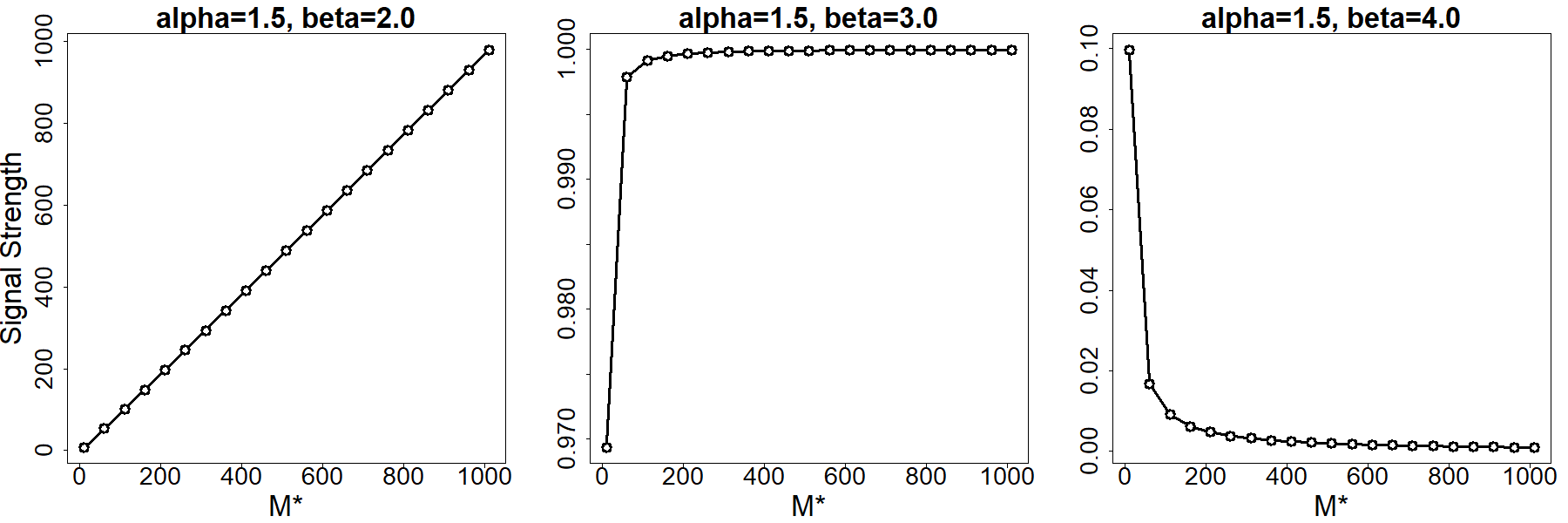
In practice, if M⋆M^{\star} is very large and we do not have enough samples to accurately estimate ΔM\Delta^{M} for a large MM, then it is impossible for us to estimate the differential graph correctly. Furthermore, the situation is worse if β>2​α\beta>2\alpha, since D12D_{12} and D23D_{23}—the signal strength—vanishes as M⋆M^{\star} increases. Figure 2 shows how the signal strength (defined as D12D_{12}) changes as M⋆M^{\star} increases for three cases: β<2​α\beta<2\alpha, β=2​α\beta=2\alpha, and β>2​α\beta>2\alpha.

This problem is intrinsically hard because the difference between two graphs occurs only between components with the smallest positive eigenvalue. To capture this difference, we have to use a large number of bases MM to approximate the functional data, which is statistically expensive. As we increase MM, no useful information is captured until M=M⋆M=M^{\star}. Furthermore, if the difference between the eigenvalues decreases quickly relative to the decrease of the eigenvalues, the signal strength will be very weak when the intrinsic dimension is large.
Refer to caption
Figure 2: Signal Strength D12≍(M⋆)−2​(β−2​α)D_{12}\asymp(M^{\star})^{-2(\beta-2\alpha)} in Example 11.

In Example 10, we characterized a pair of infinite-dimensional MGPs that are comparable, and in Example 11 we discussed a sequence of models that are all comparable, but increasingly difficult to recover. The following example demonstrates that there are infinite-dimensional MGPs that may share the same eigenspace but are still not comparable.

Example 12.

We construct two MGPs that are both infinite-dimensional and have the same eigenspace but are incomparable. As in the previous two examples, let V={1,2,3}V=\{1,2,3\}. We assume that XX and YY share a common set of eigenfunctions: {ϕm}m=1∞\{\phi_{m}\}_{m=1}^{\infty} for j=1,2,3j=1,2,3.

We construct the distribution of the scores of XX and YY as follows. For any m∈ℕ+m\in\mathbb{N}^{+}, let ai⋅mXa^{X}_{i\,\cdot\,m} denote the vector of scores (ai​1​mX,ai​2​mX,ai​3​mX)(a^{X}_{i1m},a^{X}_{i2m},a^{X}_{i3m}) and define ai⋅mYa^{Y}_{i\,\cdot\,m} analogously. For any natural number zz, we first assume that

ai⋅(3​z−2)X,ai⋅(3​z−1)X,ai⋅(3​z)X⟂⟂{ai⋅kX}k≠3​z,3​z−1,3​z−2.a^{X}_{i\,\cdot\,(3z-2)},a^{X}_{i\,\cdot\,(3z-1)},a^{X}_{i\,\cdot\,(3z)}\perp\!\!\!\perp\{a^{X}_{i\,\cdot\,k}\}_{k\neq 3z,3z-1,3z-2}. (17)

Thus, the conditional independence graph for individual scores is a set of disconnected subgraphs corresponding to {ai⋅(3​z−2)X,ai⋅,(3z−1)X,ai⋅(3​z)X}\{a^{X}_{i\,\cdot\,(3z-2)},a^{X}_{i\,\cdot,(3z-1)},a^{X}_{i\,\cdot\,(3z)}\} for z∈ℕ+z\in\mathbb{N}^{+}. We make an analogous assumption for the scores of YY.

Within sets {ai⋅(3​z−2)X,ai⋅(3​z−1)X,ai⋅(3​z)X}\{a^{X}_{i\,\cdot\,(3z-2)},a^{X}_{i\,\cdot\,(3z-1)},a^{X}_{i\,\cdot\,(3z)}\} and {ai⋅(3​z−2)Y,ai⋅(3​z−1)Y,ai⋅(3​z)Y}\{a^{Y}_{i\,\cdot\,(3z-2)},a^{Y}_{i\,\cdot\,(3z-1)},a^{Y}_{i\,\cdot\,(3z)}\}, we assume that the conditional independence graph has the structure shown in Figure 3. By construction, when projecting onto the span of the first MM functions, the edge set of individual functional graphical models for XπX^{\pi} and YπY^{\pi} is not stable as M→∞M\rightarrow\infty. In particular, for both XX and YY, the edges (1,2)(1,2) and (2,3)(2,3) will persist; however, the edge (1,3)(1,3) will appear or disappear depending on MM.

ai​1​(3​z−2)Xa^{X}_{i1(3z-2)}ai​2​(3​z−2)Xa^{X}_{i2(3z-2)}ai​3​(3​z−2)Xa^{X}_{i3(3z-2)}ai​1​(3​z−1)Xa^{X}_{i1(3z-1)}ai​2​(3​z−1)Xa^{X}_{i2(3z-1)}ai​3​(3​z−1)Xa^{X}_{i3(3z-1)}ai​1​(3​z)Xa^{X}_{i1(3z)}ai​2​(3​z)Xa^{X}_{i2(3z)}ai​3​(3​z)Xa^{X}_{i3(3z)}
(a) CI graph for XX scores

    ai​1​(3​z−2)Ya^{Y}_{i1(3z-2)}ai​2​(3​z−2)Ya^{Y}_{i2(3z-2)}ai​3​(3​z−2)Ya^{Y}_{i3(3z-2)}ai​1​(3​z−1)Ya^{Y}_{i1(3z-1)}ai​2​(3​z−1)Ya^{Y}_{i2(3z-1)}ai​3​(3​z−1)Ya^{Y}_{i3(3z-1)}ai​1​(3​z)Ya^{Y}_{i1(3z)}ai​2​(3​z)Ya^{Y}_{i2(3z)}ai​3​(3​z)Ya^{Y}_{i3(3z)} (b) CI graph for YY scores

Figure 3: CI graph for the individual scores for two incomparable MGPs.

If M=3​z−2M=3z-2 for some z∈ℕ+z\in\mathbb{N}^{+}, which corresponds to the first row in Figure 3, then

{ai​1​kX}k<M⟂⟂{ai​3​kX}k<M|{ai​2​kX}k≤M and {ai​1​kY}k<M⟂⟂{ai​3​kY}k<M|{ai​2​kY}k≤M.\{a^{X}_{i1k}\}_{k<M}\perp\!\!\!\perp\{a^{X}_{i3k}\}_{k<M}\mid\{a^{X}_{i2k}\}_{k\leq M}\quad\text{ and }\quad\{a^{Y}_{i1k}\}_{k<M}\perp\!\!\!\perp\{a^{Y}_{i3k}\}_{k<M}\mid\{a^{Y}_{i2k}\}_{k\leq M}. (18)

However, ai​1​MX⟂̸⟂ai​3​MX|{ai​2​kX}k≤Ma^{X}_{i1M}\not\perp\!\!\!\perp a^{X}_{i3M}\mid\{a^{X}_{i2k}\}_{k\leq M} since we do not condition on ai​2​(M+1)Xa^{X}_{i2(M+1)}. Similarly, ai​1​MY⟂̸⟂ai​3​MY|{ai​2​kY}k≤Ma^{Y}_{i1M}\not\perp\!\!\!\perp a^{Y}_{i3M}\mid\{a^{Y}_{i2k}\}_{k\leq M} since we do not condition on ai​2​(M+2)Ya^{Y}_{i2(M+2)}. Thus, the edge (1,3)(1,3) is in the functional graphical model for both XπX^{\pi} and YπY^{\pi}; however, the specific values of ΘX,M\Theta^{X,M} and ΘY,M\Theta^{Y,M} may differ.

In contrast to the previous case, when M=3​z−1M=3z-1 for some z∈ℕ+z\in\mathbb{N}^{+}, which corresponds to the second row of Figure 3, the functional graphical models for XπX^{\pi} and YπY^{\pi} now differ. Note that {ai​1​kX}k≤M⟂⟂{ai​3​kX}k≤M|{ai​2​kX}k≤M\{a^{X}_{i1k}\}_{k\leq M}\perp\!\!\!\perp\{a^{X}_{i3k}\}_{k\leq M}\mid\{a^{X}_{i2k}\}_{k\leq M}. Thus, the edge (1,3)(1,3) is absent from the functional graphical model for XπX^{\pi} and Θ1,3X,M=0\Theta^{X,M}_{1,3}=0. Considering YπY^{\pi}, we have {ai​1​kY}k<M−1⟂⟂{ai​3​kY}k<M−1|{ai​2​kY}k≤M\{a^{Y}_{i1k}\}_{k<M-1}\perp\!\!\!\perp\{a^{Y}_{i3k}\}_{k<M-1}\mid\{a^{Y}_{i2k}\}_{k\leq M}. However, because we do not condition on ai​2​(M+1)Ya^{Y}_{i2(M+1)} (the node in the third row of Figure 3), the (1,3)(1,3) edge exists in the functional graphical model for YπY^{\pi} since ai​1​(M−1)Y⟂̸⟂ai​3​(M−1)Y|{ai​2​kY}k≤Ma^{Y}_{i1(M-1)}\not\perp\!\!\!\perp a^{Y}_{i3(M-1)}\mid\{a^{Y}_{i2k}\}_{k\leq M}.

Suppose that the covariance of the scores is

z−β×   [aYi​1​(3​z−2)aYi​1​(3​z−1)aYi​1​(3​z)aYi​2​(3​z−2)aYi​2​(3​z−1)aYi​2​(3​z)aYi​3​(3​z−2)aYi​3​(3​z−1)aYi​3​(3​z)aYi​1​(3​z−2)3/20000−11/200aYi​1​(3​z−1)010000000aYi​1​(3​z)001000000aYi​2​(3​z−2)000800000aYi​2​(3​z−1)000040000aYi​2​(3​z)−101002−100aYi​3​(3​z−2)1/20000−13/200aYi​3​(3​z−1)000000010aYi​3​(3​z)000000001]  ,z^{-\beta}\times\hbox{}\vbox{\kern 0.86108pt\hbox{$\kern 0.0pt\kern 2.5pt\kern-5.0pt\left[\kern 0.0pt\kern-2.5pt\kern-5.55557pt\vbox{\kern-0.86108pt\vbox{\vbox{\halign{\kern\arraycolsep\hfil\@arstrut$\kbcolstyle#$\hfil\kern\arraycolsep& \kern\arraycolsep\hfil$\@kbrowstyle#$\ifkbalignright\relax\else\hfil\fi\kern\arraycolsep&& \kern\arraycolsep\hfil$\@kbrowstyle#$\ifkbalignright\relax\else\hfil\fi\kern\arraycolsep\cr 5.0pt\hfil\hbox{\vrule height=0.0pt,depth=0.0pt,width=0.0pt}$\scriptstyle$\hfil\kern 5.0pt&5.0pt\hfil$\scriptstyle a^{Y}_{i1(3z-2)}$\hfil\kern 5.0pt&5.0pt\hfil$\scriptstyle a^{Y}_{i1(3z-1)}$\hfil\kern 5.0pt&5.0pt\hfil$\scriptstyle a^{Y}_{i1(3z)}$\hfil\kern 5.0pt&5.0pt\hfil$\scriptstyle a^{Y}_{i2(3z-2)}$\hfil\kern 5.0pt&5.0pt\hfil$\scriptstyle a^{Y}_{i2(3z-1)}$\hfil\kern 5.0pt&5.0pt\hfil$\scriptstyle a^{Y}_{i2(3z)}$\hfil\kern 5.0pt&5.0pt\hfil$\scriptstyle a^{Y}_{i3(3z-2)}$\hfil\kern 5.0pt&5.0pt\hfil$\scriptstyle a^{Y}_{i3(3z-1)}$\hfil\kern 5.0pt&5.0pt\hfil$\scriptstyle a^{Y}_{i3(3z)}$\hfil\kern 5.0pt\\ 5.0pt\hfil\hbox{\vrule height=0.0pt,depth=0.0pt,width=0.0pt}$\scriptstyle a^{Y}_{i1(3z-2)}$\hfil\kern 5.0pt&5.0pt\hfil$\scriptstyle 3/2$\hfil\kern 5.0pt&5.0pt\hfil$\scriptstyle 0$\hfil\kern 5.0pt&5.0pt\hfil$\scriptstyle 0$\hfil\kern 5.0pt&5.0pt\hfil$\scriptstyle 0$\hfil\kern 5.0pt&5.0pt\hfil$\scriptstyle 0$\hfil\kern 5.0pt&5.0pt\hfil$\scriptstyle-1$\hfil\kern 5.0pt&5.0pt\hfil$\scriptstyle 1/2$\hfil\kern 5.0pt&5.0pt\hfil$\scriptstyle 0$\hfil\kern 5.0pt&5.0pt\hfil$\scriptstyle 0$\hfil\kern 5.0pt\\ 5.0pt\hfil\hbox{\vrule height=0.0pt,depth=0.0pt,width=0.0pt}$\scriptstyle a^{Y}_{i1(3z-1)}$\hfil\kern 5.0pt&5.0pt\hfil$\scriptstyle 0$\hfil\kern 5.0pt&5.0pt\hfil$\scriptstyle 1$\hfil\kern 5.0pt&5.0pt\hfil$\scriptstyle 0$\hfil\kern 5.0pt&5.0pt\hfil$\scriptstyle 0$\hfil\kern 5.0pt&5.0pt\hfil$\scriptstyle 0$\hfil\kern 5.0pt&5.0pt\hfil$\scriptstyle 0$\hfil\kern 5.0pt&5.0pt\hfil$\scriptstyle 0$\hfil\kern 5.0pt&5.0pt\hfil$\scriptstyle 0$\hfil\kern 5.0pt&5.0pt\hfil$\scriptstyle 0$\hfil\kern 5.0pt\\ 5.0pt\hfil\hbox{\vrule height=0.0pt,depth=0.0pt,width=0.0pt}$\scriptstyle a^{Y}_{i1(3z)}$\hfil\kern 5.0pt&5.0pt\hfil$\scriptstyle 0$\hfil\kern 5.0pt&5.0pt\hfil$\scriptstyle 0$\hfil\kern 5.0pt&5.0pt\hfil$\scriptstyle 1$\hfil\kern 5.0pt&5.0pt\hfil$\scriptstyle 0$\hfil\kern 5.0pt&5.0pt\hfil$\scriptstyle 0$\hfil\kern 5.0pt&5.0pt\hfil$\scriptstyle 0$\hfil\kern 5.0pt&5.0pt\hfil$\scriptstyle 0$\hfil\kern 5.0pt&5.0pt\hfil$\scriptstyle 0$\hfil\kern 5.0pt&5.0pt\hfil$\scriptstyle 0$\hfil\kern 5.0pt\\ 5.0pt\hfil\hbox{\vrule height=0.0pt,depth=0.0pt,width=0.0pt}$\scriptstyle a^{Y}_{i2(3z-2)}$\hfil\kern 5.0pt&5.0pt\hfil$\scriptstyle 0$\hfil\kern 5.0pt&5.0pt\hfil$\scriptstyle 0$\hfil\kern 5.0pt&5.0pt\hfil$\scriptstyle 0$\hfil\kern 5.0pt&5.0pt\hfil$\scriptstyle 8$\hfil\kern 5.0pt&5.0pt\hfil$\scriptstyle 0$\hfil\kern 5.0pt&5.0pt\hfil$\scriptstyle 0$\hfil\kern 5.0pt&5.0pt\hfil$\scriptstyle 0$\hfil\kern 5.0pt&5.0pt\hfil$\scriptstyle 0$\hfil\kern 5.0pt&5.0pt\hfil$\scriptstyle 0$\hfil\kern 5.0pt\\ 5.0pt\hfil\hbox{\vrule height=0.0pt,depth=0.0pt,width=0.0pt}$\scriptstyle a^{Y}_{i2(3z-1)}$\hfil\kern 5.0pt&5.0pt\hfil$\scriptstyle 0$\hfil\kern 5.0pt&5.0pt\hfil$\scriptstyle 0$\hfil\kern 5.0pt&5.0pt\hfil$\scriptstyle 0$\hfil\kern 5.0pt&5.0pt\hfil$\scriptstyle 0$\hfil\kern 5.0pt&5.0pt\hfil$\scriptstyle 4$\hfil\kern 5.0pt&5.0pt\hfil$\scriptstyle 0$\hfil\kern 5.0pt&5.0pt\hfil$\scriptstyle 0$\hfil\kern 5.0pt&5.0pt\hfil$\scriptstyle 0$\hfil\kern 5.0pt&5.0pt\hfil$\scriptstyle 0$\hfil\kern 5.0pt\\ 5.0pt\hfil\hbox{\vrule height=0.0pt,depth=0.0pt,width=0.0pt}$\scriptstyle a^{Y}_{i2(3z)}$\hfil\kern 5.0pt&5.0pt\hfil$\scriptstyle-1$\hfil\kern 5.0pt&5.0pt\hfil$\scriptstyle 0$\hfil\kern 5.0pt&5.0pt\hfil$\scriptstyle 1$\hfil\kern 5.0pt&5.0pt\hfil$\scriptstyle 0$\hfil\kern 5.0pt&5.0pt\hfil$\scriptstyle 0$\hfil\kern 5.0pt&5.0pt\hfil$\scriptstyle 2$\hfil\kern 5.0pt&5.0pt\hfil$\scriptstyle-1$\hfil\kern 5.0pt&5.0pt\hfil$\scriptstyle 0$\hfil\kern 5.0pt&5.0pt\hfil$\scriptstyle 0$\hfil\kern 5.0pt\\ 5.0pt\hfil\hbox{\vrule height=0.0pt,depth=0.0pt,width=0.0pt}$\scriptstyle a^{Y}_{i3(3z-2)}$\hfil\kern 5.0pt&5.0pt\hfil$\scriptstyle 1/2$\hfil\kern 5.0pt&5.0pt\hfil$\scriptstyle 0$\hfil\kern 5.0pt&5.0pt\hfil$\scriptstyle 0$\hfil\kern 5.0pt&5.0pt\hfil$\scriptstyle 0$\hfil\kern 5.0pt&5.0pt\hfil$\scriptstyle 0$\hfil\kern 5.0pt&5.0pt\hfil$\scriptstyle-1$\hfil\kern 5.0pt&5.0pt\hfil$\scriptstyle 3/2$\hfil\kern 5.0pt&5.0pt\hfil$\scriptstyle 0$\hfil\kern 5.0pt&5.0pt\hfil$\scriptstyle 0$\hfil\kern 5.0pt\\ 5.0pt\hfil\hbox{\vrule height=0.0pt,depth=0.0pt,width=0.0pt}$\scriptstyle a^{Y}_{i3(3z-1)}$\hfil\kern 5.0pt&5.0pt\hfil$\scriptstyle 0$\hfil\kern 5.0pt&5.0pt\hfil$\scriptstyle 0$\hfil\kern 5.0pt&5.0pt\hfil$\scriptstyle 0$\hfil\kern 5.0pt&5.0pt\hfil$\scriptstyle 0$\hfil\kern 5.0pt&5.0pt\hfil$\scriptstyle 0$\hfil\kern 5.0pt&5.0pt\hfil$\scriptstyle 0$\hfil\kern 5.0pt&5.0pt\hfil$\scriptstyle 0$\hfil\kern 5.0pt&5.0pt\hfil$\scriptstyle 1$\hfil\kern 5.0pt&5.0pt\hfil$\scriptstyle 0$\hfil\kern 5.0pt\\ 5.0pt\hfil\hbox{\vrule height=0.0pt,depth=0.0pt,width=0.0pt}$\scriptstyle a^{Y}_{i3(3z)}$\hfil\kern 5.0pt&5.0pt\hfil$\scriptstyle 0$\hfil\kern 5.0pt&5.0pt\hfil$\scriptstyle 0$\hfil\kern 5.0pt&5.0pt\hfil$\scriptstyle 0$\hfil\kern 5.0pt&5.0pt\hfil$\scriptstyle 0$\hfil\kern 5.0pt&5.0pt\hfil$\scriptstyle 0$\hfil\kern 5.0pt&5.0pt\hfil$\scriptstyle 0$\hfil\kern 5.0pt&5.0pt\hfil$\scriptstyle 0$\hfil\kern 5.0pt&5.0pt\hfil$\scriptstyle 0$\hfil\kern 5.0pt&5.0pt\hfil$\scriptstyle 1$\hfil\kern 5.0pt\\ }}}}\right]$}},

where β>0\beta>0 is a parameter that determines the decay rate of the eigenvalues (see Assumption 3). We then set all other elements of the covariance as 00. The support of the inverse of this matrix corresponds to the edges of the graph in Figure 3. However, when we consider the marginal distribution of the first MM scores and invert the corresponding covariance, Θ1,3Y,M\Theta^{Y,M}_{1,3} is 00 everywhere except for the element corresponding to ai,1,M−1Ya^{Y}_{i,1,M-1} and ai,3,M−1Ya^{Y}_{i,3,M-1}, that is, the nodes in the top row of Figure 3, which is equal to −1/4×((M+1)/3)β-1/4\times((M+1)/3)^{\beta}. Thus, ‖Δ1,3M‖F=1/4×((M+1)/3)β\|\Delta^{M}_{1,3}\|_{F}=1/4\times((M+1)/3)^{\beta} and limsupM→∞‖Δ1,3M‖F=∞\lim\sup_{M\rightarrow\infty}\|\Delta^{M}_{1,3}\|_{F}=\infty.

Finally, when M=3​zM=3z for some z∈ℕ+z\in\mathbb{N}^{+}, the (1,3)(1,3) edge is absent in both functional graphical models for XπX^{\pi} and YπY^{\pi} because

{ai​1​kX}k≤M⟂⟂{ai​3​kX}k≤M|{ai​2​kX}k≤M​ and ​{ai​1​kY}k≤M⟂⟂{ai​3​kY}k≤M|{ai​2​kY}k≤M.\{a^{X}_{i1k}\}_{k\leq M}\perp\!\!\!\perp\{a^{X}_{i3k}\}_{k\leq M}\mid\{a^{X}_{i2k}\}_{k\leq M}\ \text{ and }\ \{a^{Y}_{i1k}\}_{k\leq M}\perp\!\!\!\perp\{a^{Y}_{i3k}\}_{k\leq M}\mid\{a^{Y}_{i2k}\}_{k\leq M}.

Thus, Θ1,3X,M=Θ1,3Y,M=Δ1,3M=0\Theta^{X,M}_{1,3}=\Theta^{Y,M}_{1,3}=\Delta^{M}_{1,3}=0. This implies that liminfM→∞‖Δ1,3M‖F=0\lim\inf_{M\rightarrow\infty}\|\Delta^{M}_{1,3}\|_{F}=0.

Because liminfM→∞‖Δ1,3M‖F=0\lim\inf_{M\rightarrow\infty}\|\Delta^{M}_{1,3}\|_{F}=0, but limsupM→∞‖Δ1,3M‖F=∞\lim\sup_{M\rightarrow\infty}\|\Delta^{M}_{1,3}\|_{F}=\infty, XX and YY are incomparable.

The notion of comparability illustrates the intrinsic difficulty of dealing with functional data. However, it also illustrates when we can still hope to estimate the differential network consistently. We have formally stated when two infinite-dimensional functional graphical models will be comparable and have given conditions and examples of comparability. Unfortunately, these conditions cannot be checked using the observed data. For this reason, we mainly discuss the methodology and theoretical properties for estimation of EΔπE^{\pi}_{\Delta}. Prior knowledge about the problem at hand should be used to decide whether two infinite-dimensional functional graphs are comparable. This is similar to other assumptions common in the graphical modeling literature, such as “faithfulness” (Spirtes et al. 2000), that are critical to graph recovery, but can not be verified.

3 Functional Differential Graph Estimation: FuDGE

In this section, we detail our methodology for estimating a functional differential graph. Unfortunately, in most situations, there may not be prior knowledge on which subspace to use to define the functional differential graph. In such situations, we suggest using the principle component scores of Kj​j​(s,t)=Kj​jX​(s,t)+Kj​jY​(s,t)K_{jj}(s,t)=K^{X}_{jj}(s,t)+K^{Y}_{jj}(s,t), j∈Vj\in V as a default choice. In addition, each observed function is only recorded (potentially with measurement error) at discrete time points. In Section 3.1 we consider this practical setting. Of course, if an appropriate basis for dimension reduction is known in advance or if the functions are fully observed at all time points, then the estimated objects can always be replaced with their known/observed counterparts.

3.1 Estimating the Covariance of the Scores

For each Xi​jX_{ij}, suppose we have measurements at time points ti​j​kt_{ijk}, k=1,…,Tk=1,\ldots,T,33 3 For simplicity, we assume that all functions have the same number of observations, however, our method and theory can be trivially extended to allow a different number of observations for each function. and the recorded data, hi​j​kh_{ijk}, are the function values with random noise. That is,

hi​j​k=gi​j​(ti​j​k)+ϵi​j​k,h_{ijk}=g_{ij}(t_{ijk})+\epsilon_{ijk}, (19)

where gi​jg_{ij} can denote either Xi​jX_{ij} or Yi​jY_{ij} and the unobserved noise ϵi​j​k\epsilon_{ijk} is i.i.d. Gaussian with mean 00 and variance σ02\sigma^{2}_{0}. Without loss of generality, we assume that ti​j​1<…<ti​j​Tt_{ij1}<\ldots<t_{ijT} for any 1≤i≤n1\leq i\leq n and 1≤j≤p1\leq j\leq p. We do not assume that ti​j​k=ti′​j​kt_{ijk}=t_{i^{\prime}jk} for i≠i′i\neq i^{\prime}, so that each observation may be observed on a different grid.

We first use a basis expansion to estimate a least squares approximation of the whole curve Xi​j​(t)X_{ij}(t) (see Section 4.2 in Ramsay and Silverman 2005). Specifically, given an initial basis function vector b⁡(t)=(b1​(t),…,bL​(t))⊤b(t)=(b_{1}(t),\dots,b_{L}(t))^{\top}—for example, the B-spline or Fourier basis—our estimated approximation for Xi​j​(t)X_{ij}(t) is given by:

X^i​j​(t)\displaystyle\hat{X}_{ij}(t) =β^i​j⊤​b​(t),\displaystyle=\hat{\beta}_{ij}^{\top}b(t), (20)
β^i​j\displaystyle\hat{\beta}_{ij} =(Bi​j⊤​Bi​j)−1​Bi​j⊤​hi​j,\displaystyle=\left(B^{\top}_{ij}B_{ij}\right)^{-1}B^{\top}_{ij}h_{ij},

where hi​j=(hi​j​1,hi​j​2,…,hi​j​T)⊤h_{ij}=(h_{ij1},h_{ij2},\dots,h_{ijT})^{\top} and Bi​jB_{ij} is the design matrix for gi​jg_{ij}:

Bi​j=[b1​(ti​j​1)⋯bL​(ti​j​1)⋱b1​(ti​j​T)⋯bL​(ti​j​T)]∈ℝT×L.B_{ij}=\left[\begin{matrix}b_{1}(t_{ij1})&\cdots&b_{L}(t_{ij1})\\ \vdots&\ddots&\vdots\\ b_{1}(t_{ijT})&\cdots&b_{L}(t_{ijT})\end{matrix}\right]\in\mathbb{R}^{T\times L}. (21)

The computational complexity of the basis expansion procedure is O⁡(n​p​T3​L3)O(npT^{3}L^{3}), and in practice, there are many efficient package implementations of this step; for example, fda (Ramsay et al. 2020).

We repeat this process for the observed YY functions. After obtaining {X^i​j​(t)}j∈V,i=1,…,nX\{\hat{X}_{ij}(t)\}_{j\in V,i=1,\ldots,n_{X}} and {Y^i​j​(t)}j∈V,i=1,…,nY\{\hat{Y}_{ij}(t)\}_{j\in V,i=1,\ldots,n_{Y}}, we use them as inputs for the FPCA procedure. Specifically, we first estimate the sum of the covariance functions by

K^j​j​(s,t)=K^j​jX​(s,t)+K^j​jY​(s,t)=1nX​∑i=1nXX^i​j​(s)​X^i​j​(t)+1nY​∑i=1nYY^i​j​(s)​Y^i​j​(t).\hat{K}_{jj}(s,t)=\hat{K}^{X}_{jj}(s,t)+\hat{K}^{Y}_{jj}(s,t)=\frac{1}{n_{X}}\sum^{n_{X}}_{i=1}\hat{X}_{ij}(s)\hat{X}_{ij}(t)+\frac{1}{n_{Y}}\sum^{n_{Y}}_{i=1}\hat{Y}_{ij}(s)\hat{Y}_{ij}(t). (22)

Using K^j​j​(s,t)\hat{K}_{jj}(s,t) as input to FPCA, we can estimate the corresponding eigenfunctions ϕ^j​k​(t)\hat{\phi}_{jk}(t), k=1,…,Mk=1,\ldots,M, j=1,…,pj=1,\ldots,p. Given the estimated eigenfunctions, we compute the estimated projection scores

a^i​j​kX\displaystyle\hat{a}^{X}_{ijk} =∫𝒯X^i​j(t)ϕ^j​k(t)dtanda^i​j​kY=∫𝒯Yi​j(t)ϕ^j​k(t)dt,\displaystyle=\int_{\mathcal{T}}\hat{X}_{ij}(t)\hat{\phi}_{jk}(t)dt\qquad\text{and}\qquad\hat{a}^{Y}_{ijk}=\int_{\mathcal{T}}Y_{ij}(t)\hat{\phi}_{jk}(t)dt,

and collect them into vectors

a^i​jX,M\displaystyle\hat{a}^{X,M}_{ij} =(a^i​j​1X,⋯,a^i​j​MX)⊤∈ℝManda^iX,M\displaystyle=(\hat{a}^{X}_{ij1},\cdots,\hat{a}^{X}_{ijM})^{\top}\in{\mathbb{R}^{M}}\qquad\text{and}\qquad\hat{a}^{X,M}_{i} =((a^i​1X,M)⊤,…,(a^i​pX,M)⊤)⊤∈ℝp​M,\displaystyle=((\hat{a}^{X,M}_{i1})^{\top},\ldots,(\hat{a}^{X,M}_{ip})^{\top})^{\top}\in{\mathbb{R}^{pM}},
a^i​jY,M\displaystyle\hat{a}^{Y,M}_{ij} =(a^i​j​1Y,⋯,a^i​j​MY)⊤∈ℝManda^iY,M\displaystyle=(\hat{a}^{Y}_{ij1},\cdots,\hat{a}^{Y}_{ijM})^{\top}\in{\mathbb{R}^{M}}\qquad\text{and}\qquad\hat{a}^{Y,M}_{i} =((a^i​1Y,M)⊤,…,(a^i​pY,M)⊤)⊤∈ℝp​M.\displaystyle=((\hat{a}^{Y,M}_{i1})^{\top},\ldots,(\hat{a}^{Y,M}_{ip})^{\top})^{\top}\in{\mathbb{R}^{pM}}.

Finally, we estimate the covariance matrices of the score vectors, ΣX,M\Sigma^{X,M} and ΣY,M\Sigma^{Y,M}, as

SX,M=1nX​∑i=1nXa^iX,M​(a^iX,M)⊤andSY,M=1nY​∑i=1nYa^iY,M​(a^iY,M)⊤.\displaystyle S^{X,M}=\frac{1}{n_{X}}\sum^{n_{X}}_{i=1}\hat{a}^{X,M}_{i}(\hat{a}^{X,M}_{i})^{\top}\qquad\text{and}\qquad S^{Y,M}=\frac{1}{n_{Y}}\sum^{n_{Y}}_{i=1}\hat{a}^{Y,M}_{i}(\hat{a}^{Y,M}_{i})^{\top}.

3.2 FuDGE: Functional Differential Graph Estimation

Now we describe the FuDGE algorithm for Functional Differential Graph Estimation. To estimate ΔM\Delta^{M}, we solve the following optimization program:

Δ^M∈arg​minΔ∈ℝpM×pM⁡ℒ​(Δ)+λn​∑{i,j}∈V2‖Δij‖F,\hat{\Delta}^{M}\in\argmin_{\Delta\in{\mathbb{R}^{pM\times pM}}}\mathcal{L}(\Delta)+\lambda_{n}\sum_{\{i,j\}\in V^{2}}\|\Delta_{ij}\|_{F}, (23)

where

ℒ⁡(Δ)=tr⁡[12​SY,M​Δ⊤​SX,M​Δ−Δ⊤​(SY,M−SX,M)]\mathcal{L}(\Delta)=\mathrm{tr}\left[\frac{1}{2}S^{Y,M}\Delta^{\top}{S^{X,M}}\Delta-\Delta^{\top}\left(S^{Y,M}-S^{X,M}\right)\right] (24)

and SX,MS^{X,M} and SY,MS^{Y,M} are obtained as described in Section 3.1.

We construct the loss function, ℒ⁡(Δ)\mathcal{L}(\Delta), so that the true parameter value, that is, ΔM=(ΣX,M)−1−(ΣY,M)−1\Delta^{M}=\left(\Sigma^{X,M}\right)^{-1}-\left(\Sigma^{Y,M}\right)^{-1}, minimizes the population loss 𝔼⁡[ℒ⁡(Δ)]\mathbb{E}\left[\mathcal{L}(\Delta)\right], which for a differentiable and convex loss function is equivalent to selecting ℒ\mathcal{L} so that 𝔼⁡[∇ℒ​(ΔM)]=0\mathbb{E}\left[\nabla\mathcal{L}(\Delta^{M})\right]=0. Since ΔM\Delta^{M} satisfies

ΣX,M​ΔM​ΣY,M−(ΣY,M−ΣX,M)=0,\Sigma^{X,M}\Delta^{M}\Sigma^{Y,M}-(\Sigma^{Y,M}-\Sigma^{X,M})=0,

a choice for ∇ℒ​(Δ)\nabla\mathcal{L}(\Delta) is

∇ℒ​(ΔM)=SX,M​ΔM​SY,M−(SY,M−SX,M)\nabla{\mathcal{L}(\Delta^{M})}=S^{X,M}\Delta^{M}{S^{Y,M}}-\left(S^{Y,M}-S^{X,M}\right) (25)

so that

𝔼⁡[∇ℒ​(ΔM)]=ΣX,M​ΔM​ΣY,M−(ΣY,M−ΣX,M)=0.\mathbb{E}\left[\nabla\mathcal{L}(\Delta^{M})\right]=\Sigma^{X,M}\Delta^{M}\Sigma^{Y,M}-(\Sigma^{Y,M}-\Sigma^{X,M})=0.

Given this choice of ∇ℒ​(Δ)\nabla\mathcal{L}(\Delta), ℒ⁡(Δ)\mathcal{L}(\Delta) in (23) directly follows from properties of the differential of the trace function. The chosen loss is quadratic (see (B.9) in appendix) and leads to an efficient algorithm. Similar loss functions are used in Xu and Gu 2016, Yuan et al. 2017, Na et al. 2021, and Zhao et al. 2014a.

We also include the additional group lasso penalty (Yuan and Lin 2006) to promote blockwise sparsity in Δ^M\hat{\Delta}^{M}. The objective in (23) can be solved by a proximal gradient method detailed in Algorithm 1. Finally, we form E^Δ\hat{E}_{\Delta} by thresholding Δ^M\hat{\Delta}^{M} so that:

E^Δ={{j,l}:‖Δ^j​lM‖F>ϵn​or​‖Δ^l​jM‖F>ϵn}.{}\hat{E}_{\Delta}=\left\{\{j,l\}\,:\,\|\hat{\Delta}^{M}_{jl}\|_{F}>\epsilon_{n}\;\;\text{or}\;\;\|\hat{\Delta}^{M}_{lj}\|_{F}>\epsilon_{n}\right\}. (26)

The thresholding step in (26) is used for theoretical purposes. Specifically, it helps correct for bias induced by finite-dimensional truncation and relaxes commonly used assumptions for the recovery of the graph structure, such as the irrepresentability or incoherence condition (van de Geer and Bühlmann 2009). In practice, one can simply set ϵn=0\epsilon_{n}=0, as we do in the simulations.

3.3 Optimization Algorithm for FuDGE

Algorithm 1 Functional differential graph estimation
0:  SX,M,SY,M,λn,ηS^{X,M},S^{Y,M},\lambda_{n},\eta.
0:  Δ^M\hat{\Delta}^{M}.
 Initialize Δ(0)=0p​M\Delta^{(0)}=0_{pM}.
 repeat
  A=Δ−η∇ℒ(Δ)=Δ−η(SX,MΔSY,M−(SY,M−SX,M))A=\Delta-\eta\nabla\mathcal{L}(\Delta)=\Delta-\eta\left(S^{X,M}\Delta S^{Y,M}-\left(S^{Y,M}-S^{X,M}\right)\right)
  for 1≤i,j≤p1\leq{i,j}\leq{p} do
   Δj​l←(‖Aj​l‖F−λn​η‖Aj​l‖F)+⋅Aj​l\Delta_{jl}\leftarrow\left(\frac{\|A_{jl}\|_{F}-\lambda_{n}\eta}{\|A_{jl}\|_{F}}\right)_{+}\cdot A_{jl}
  end for
 until Converge

The optimization program (23) can be solved using a proximal gradient method (Parikh and Boyd 2014) summarized in Algorithm 1. Specifically, at each iteration, we update the current value of Δ\Delta, denoted as Δold\Delta^{\text{old}}, by solving the following problem:

Δnew=arg​minΔ(12‖Δ−(Δold−η∇ℒ(Δold))‖F2+η⋅λn∑j,l=1p∥Δjl∥F),{}\Delta^{\text{new}}=\argmin_{\Delta}\left(\frac{1}{2}\left\|\Delta-\left(\Delta^{\text{old}}-\eta\nabla\mathcal{L}\left(\Delta^{\text{old}}\right)\right)\right\|_{F}^{2}+\eta\cdot\lambda_{n}\sum^{p}_{j,l=1}\|\Delta_{jl}\|_{F}\right), (27)

where ∇ℒ​(Δ)\nabla\mathcal{L}(\Delta) is defined in (25) and η\eta is a step size specified by the user. Note that ∇ℒ​(Δ)\nabla\mathcal{L}(\Delta) is Lipschitz continuous with Lipschitz constant λmaxS=‖SY,M⊗SX,M‖2=λmax​(SY,M)​λmax​(SX,M)\lambda^{S}_{\max}=\|S^{Y,M}\otimes S^{X,M}\|_{2}=\lambda_{\max}(S^{Y,M})\lambda_{\max}(S^{X,M}). Thus, for any step size η\eta such that 0<η≤1/λmaxS0<\eta\leq 1/\lambda^{S}_{\max}, the proximal gradient method is guaranteed to converge (Beck and Teboulle 2009).

The update in (27) has a closed-form solution:

Δj​lnew=[(‖Aj​lold‖F−λn​η)/‖Aj​lold‖F]+⋅Aj​lold,1≤j,l≤p,{}\Delta^{\text{new}}_{jl}=\left[\left(\|A^{\text{old}}_{jl}\|_{F}-\lambda_{n}\eta\right)/\|A^{\text{old}}_{jl}\|_{F}\right]_{+}\cdot A^{\text{old}}_{jl},\qquad 1\leq{j,l}\leq{p}, (28)

where Aold=Δold−η∇ℒ(Δold)A^{\text{old}}=\Delta^{\text{old}}-\eta\nabla\mathcal{L}(\Delta^{\text{old}}) and x+=max⁡{0,x},x∈ℝx_{+}=\max\{0,x\},x\in{\mathbb{R}}, represents the positive part of xx. Detailed derivations are given in the appendix. Note that although true ΔM\Delta^{M} is symmetric, we do not explicitly enforce symmetry in Δ^M\hat{\Delta}^{M} in Algorithm 1.

After performing FPCA, the proximal gradient descent method converges in O⁡(λmaxS/tol)O\left(\lambda^{S}_{\max}/\text{tol}\right) iterations, where tol is a user specified optimization error tolerance, and each iteration takes O⁡((p​M)3)O((pM)^{3}) operations; see Tibshirani 2010 for a convergence analysis of the general proximal gradient descent algorithm.

3.4 Selection of Tuning Parameters

There are four tuning parameters that must be chosen for the implementation of FuDGE: LL (basis dimension used to estimate the curves from the discretely observed data), MM (subspace dimension to estimate projection scores), λn\lambda_{n} (regularization parameter to tune the block sparsity of ΔM\Delta^{M}), and ϵn\epsilon_{n} (thresholding parameter for E^Δ\hat{E}_{\Delta}). While we need the thresholding parameter ϵn\epsilon_{n} in (26) to establish theoretical results, in practice, we simply set ϵn=0\epsilon_{n}=0. To select MM, we follow the procedure in Qiao et al. 2019. More specifically, for each discretely-observed curve, we first estimate the underlying functions by fitting an LL-dimensional B-spline basis. Both MM and LL are chosen by 5-fold cross-validation as discussed in Qiao et al. 2019.

Finally, to choose λn\lambda_{n}, we recommend using selective cross-validation (SCV) (She 2012). Given a value of λn\lambda_{n}, we use the entire data set to estimate a sparsity pattern. Then, fixing the sparsity pattern, we use a typical cross-validation procedure to calculate the CV error, where the CV error is measured by an unpenalized version of the loss function in (24) on the held-out data set. Ultimately, we choose the value of λn\lambda_{n} that results in the sparsity pattern that minimizes CV error. In addition to SCV, if we have prior knowledge about the number of edges in the differential graph, we can also choose λn\lambda_{n} which results in the desired level of sparsity of the differential graph.

4 Theoretical Properties

In this section, we provide theoretical guarantees for FuDGE. We first give a deterministic result for E^Δ\hat{E}_{\Delta} defined in (26) when the max-norm of the difference between the estimates SX,M,SY,MS^{X,M},S^{Y,M} and their corresponding parameters, ΣX,M,ΣY,M\Sigma^{X,M},\Sigma^{Y,M}, is bounded by δn\delta_{n}. We then show that when projecting the data onto either a fixed basis or an estimated basis—under some mild conditions—δn\delta_{n} can be controlled and the bias of the finite-dimensional projection decreases fast enough that EΔE_{\Delta} can be consistently recovered.

4.1 Deterministic Guarantees for E^Δ\hat{E}_{\Delta}

In this section, we assume that SX,M,SY,MS^{X,M},S^{Y,M} are good estimates of ΣX,M,ΣY,M\Sigma^{X,M},\Sigma^{Y,M} and give a deterministic result in Theorem 13. Let n=min⁡{nX,nY}n=\min\{n_{X},n_{Y}\}. We assume that the following holds.

Assumption 1.

The matrices SX,M,SY,MS^{X,M},S^{Y,M} are estimates of ΣX,M,ΣY,M\Sigma^{X,M},\Sigma^{Y,M} that satisfy

max⁡{|SX,M−ΣX,M|∞,|SY,M−ΣY,M|∞}≤δn.\max\left\{|S^{X,M}-\Sigma^{X,M}|_{\infty},|S^{Y,M}-\Sigma^{Y,M}|_{\infty}\right\}\leq\delta_{n}. (29)

We also require that EΔE_{\Delta} be sparse. This does not preclude the case where EXE_{X} and EYE_{Y} are dense, as long as there are not too many differences in the precision matrices. This assumption is also required when estimating a differential graph from vector-valued data; for example, see Condition 1 in Zhao et al. 2014a.

Assumption 2.

There are ss edges in the differential graph; that is, |EΔ|=s|E_{\Delta}|=s and s≪ps\ll p.

We introduce the following three quantities that characterize the problem instance and will be used in Theorem 13 below:

ν1=ν1​(M)=min(j,l)∈EΔ⁡‖Δj​lM‖F,ν2=ν2​(M)=max(j,l)∈EΔC⁡‖Δj​lM‖F,\nu_{1}=\nu_{1}(M)=\min_{(j,l)\in E_{\Delta}}\|\Delta^{M}_{jl}\|_{F},\quad\nu_{2}=\nu_{2}(M)=\max_{(j,l)\in E^{C}_{\Delta}}\|\Delta^{M}_{jl}\|_{F},

and

τ=τ⁡(M)=ν1​(M)−ν2​(M).\tau=\tau(M)=\nu_{1}(M)-\nu_{2}(M). (30)

Roughly speaking, ν1​(M)\nu_{1}(M) indicates the “signal strength” present when we use the MM-dimensional representation and ν2​(M)\nu_{2}(M) measures the bias. By Definition 4, when XX and YY are comparable, we have liminfM→M⋆ν1​(M)>0\lim\inf_{M\to M^{\star}}\nu_{1}(M)>0 and limM→M⋆ν2​(M)=0\lim_{M\to M^{\star}}\nu_{2}(M)=0. Therefore, for a sufficiently large MM, we have τ>0\tau>0. However, a smaller τ\tau implies that the differential graph is harder to recover.

Before we give the deterministic result in Theorem 13, we first define additional quantities that will be used in subsequent results. Let

σmax\displaystyle\sigma_{\max} =max⁡{|ΣX,M|∞,|ΣY,M|∞},\displaystyle=\max\{|\Sigma^{X,M}|_{\infty},|\Sigma^{Y,M}|_{\infty}\}, (31)
λmin∗\displaystyle\lambda^{*}_{\min} =λmin​(ΣX,M)×λmin​(ΣY,M), and\displaystyle=\lambda_{\min}\left(\Sigma^{X,M}\right)\times\lambda_{\min}\left(\Sigma^{Y,M}\right),\text{ and }
Γn2\displaystyle\Gamma^{2}_{n} =9​λn2​sκℒ2+2​λnκℒ​(ωℒ2+2​p2​ν2),\displaystyle=\frac{9\lambda^{2}_{n}s}{\kappa^{2}_{\mathcal{L}}}+\frac{2\lambda_{n}}{\kappa_{\mathcal{L}}}(\omega^{2}_{\mathcal{L}}+2p^{2}\nu_{2}),

where

λn\displaystyle\lambda_{n} = 2​M​[(δn2+2​δn​σmax)​|ΔM|1+2​δn],\displaystyle=\;2M\left[\left(\delta_{n}^{2}+2\delta_{n}\sigma_{\max}\right)\left|\Delta^{M}\right|_{1}+2\delta_{n}\right], (32)
κℒ\displaystyle\kappa_{\mathcal{L}} =(1/2)​λmin∗−8​M2​s​(δn2+2​δn​σmax),\displaystyle=\;(1/2)\lambda^{*}_{\min}-8M^{2}s\left(\delta_{n}^{2}+2\delta_{n}\sigma_{\max}\right),
ωℒ\displaystyle\omega_{\mathcal{L}} = 4​M​p2​ν2​δn2+2​δn​σmax,\displaystyle=\;4Mp^{2}\nu_{2}\sqrt{\delta_{n}^{2}+2\delta_{n}\sigma_{\max}},

and δn\delta_{n} is defined in Assumption 1. Note that Γn\Gamma_{n}—which measures the estimation error of ‖Δ^M−ΔM‖F\|\hat{\Delta}^{M}-\Delta^{M}\|_{\text{F}}—implicitly depends on δn\delta_{n} through λn\lambda_{n}, κℒ\kappa_{\mathcal{L}}, and ωℒ\omega_{\mathcal{L}}. We observe that Γn\Gamma_{n} decreases to zero as δn\delta_{n} goes to zero. The quantity κℒ\kappa_{\mathcal{L}} is the maximum restricted eigenvalue from the analysis framework of Negahban et al. 2012. Finally, ωℒ\omega_{\mathcal{L}} is the tolerance parameter that comes from the fact that ν2\nu_{2} could be larger than zero, and will decrease to zero as ν2\nu_{2} goes to zero.

Theorem 13.

Given Assumptions 1 and 2, when ν1​(M),ν2​(M),δn,λn,σmax,M\nu_{1}(M),\nu_{2}(M),\delta_{n},\lambda_{n},\sigma_{\max},M and ss satisfy

0<Γn<τ/2andδn<(1/4)​(λmin∗+16​M2​s​(σmax)2)/(M2​s)−σmax,\displaystyle 0<\Gamma_{n}<\tau/2\qquad\text{and}\qquad\delta_{n}<(1/4)\sqrt{\left(\lambda^{*}_{\min}+16M^{2}s(\sigma_{\max})^{2}\right)/\left(M^{2}s\right)}-\sigma_{\max}, (33)

then setting ϵn∈[ν2+Γn,ν1−Γn)\epsilon_{n}\in\left[\nu_{2}+\Gamma_{n},\nu_{1}-\Gamma_{n}\right) ensures that E^Δ=EΔ\hat{E}_{\Delta}=E_{\Delta}.

As shown in Section 4.2, under some additional conditions, Assumption 1 holds for a sequence of δn\delta_{n} that decreases to 00 as nn goes to infinity. Thus, as MM and nn both increase to infinity, we have ν2+Γn≈0\nu_{2}+\Gamma_{n}\approx 0 and ν1−Γn≈min(j,l)∈EΔ⁡Dj​l\nu_{1}-\Gamma_{n}\approx\min_{(j,l)\in E_{\Delta}}D_{jl}, and we only require 0≤ϵn<min(j,l)∈EΔ⁡Dj​l0\leq\epsilon_{n}<\min_{(j,l)\in E_{\Delta}}D_{jl}.

4.2 Theoretical Guarantees for SX,MS^{X,M} and SY,MS^{Y,M}

In this section, we prove that under some mild conditions, (29) will hold with a high probability for specific values of δn\delta_{n}. We discuss the results in two cases: the case where the curves are fully observed and the case where the curves are only observed at discrete time points.

4.2.1 Fully Observed Curves

In this section, we discuss the case where each curve is fully observed. We first consider the case where the basis defining the differential graph is known in advance; that is, the exact form of {ej​k}k≥1\{e_{jk}\}_{k\geq 1} for all j∈Vj\in V is known. In this case, the projection score vectors aiX,Ma^{X,M}_{i} and aiY,Ma^{Y,M}_{i} can be recovered exactly for all i=1,2,…,ni=1,2,\dots,n. By the assumption that Xi​(t)X_{i}(t) and Yi​(t)Y_{i}(t) are pp-dimensional multivariate Gaussian processes with mean zero, we then have aiX,M∼N⁡(0,ΣX,M)a^{X,M}_{i}\sim N(0,\Sigma^{X,M}) and aiY,M∼N⁡(0,ΣY,M)a^{Y,M}_{i}\sim N(0,\Sigma^{Y,M}). The following result follows directly from the standard results on the sample covariance of multivariate Gaussian variables.

Theorem 14.

Assume that SX,MS^{X,M} and SY,MS^{Y,M} are computed as in Section 3.1, except that the basis functions {ej​k}k≥1\{e_{jk}\}_{k\geq 1}, j∈Vj\in V, are fixed and known in advance. Recall that

n=min⁡{nX,nY}andσmax=max⁡{|ΣX,M|∞,|ΣY,M|∞}.n=\min\{n_{X},n_{Y}\}\quad\text{and}\quad\sigma_{\max}=\max\{|\Sigma^{X,M}|_{\infty},|\Sigma^{Y,M}|_{\infty}\}.

Fix ι∈(0,1]\iota\in(0,1]. Suppose that nn is large enough so that

δn=σmax​C1n​log⁡(8​p2​M2ι)≤C2,\delta_{n}=\sigma_{\max}\sqrt{\frac{C_{1}}{n}\log\left(\frac{8p^{2}M^{2}}{\iota}\right)}\leq C_{2},

for some universal constants C1,C2>0C_{1},C_{2}>0. Then (29) holds with probability at least 1−ι1-\iota.

Proof.

The proof follows directly from Lemma 1 of Ravikumar et al. 2011 and a union bound. ∎

With fully observed curves and known basis functions, it follows from Theorem 14 that (1) is satisfied for δn≍log⁡(p2​M2)/n\delta_{n}\asymp\sqrt{\log(p^{2}M^{2})/n} with high probability. As assumed in Section 2.2 (and also in Qiao et al. 2019), when λj​m′X=λj​m′Y=0\lambda^{X}_{jm^{\prime}}=\lambda^{Y}_{jm^{\prime}}=0 for all jj and m′>Mm^{\prime}>M (where MM is allowed to grow with nn), then ν2​(M)=0\nu_{2}(M)=0, τ⁡(M)=ν1​(M)=min(j,l)∈EΔ⁡Dj​l>0\tau(M)=\nu_{1}(M)=\min_{(j,l)\in E_{\Delta}}D_{jl}>0, and EΔ=EΔπE_{\Delta}=E^{\pi}_{\Delta}. We can recover EΔE_{\Delta} with high probability even in the high-dimensional setting, as long as

max⁡{s​M2​log⁡(p2​M2)​|ΔM|12/((λmin⋆)2​τ2)n,s​M2​log⁡(p2​M2)/λmin⋆n}→0.\max\left\{\frac{sM^{2}\log(p^{2}M^{2})|\Delta^{M}|_{1}^{2}/((\lambda^{\star}_{\min})^{2}\tau^{2})}{n},\frac{sM^{2}\log(p^{2}M^{2})/\lambda^{\star}_{\min}}{n}\right\}\rightarrow 0.

Even with an infinite number of positive eigenvalues, high-dimensional consistency is still possible for quickly increasing ν1\nu_{1} and quickly decaying ν2\nu_{2}.

We then consider the case where the curves are fully observed, but we do not have any prior knowledge on which orthonormal function basis should be used. In this case, as discussed in Section 2.3, we recommend using the eigenfunctions of Kj​j​(⋅,∗)=Kj​jX​(⋅,∗)+Kj​jY​(⋅,∗)K_{jj}(\cdot,*)=K^{X}_{jj}(\cdot,*)+K^{Y}_{jj}(\cdot,*) as basis functions. We use FPCA to estimate the eigenfuctions of Kj​j​(⋅,∗)K_{jj}(\cdot,*) and make the following assumption.

Assumption 3.

Let {λj​k,ϕj​k​(⋅)}\{\lambda_{jk},\phi_{jk}(\cdot)\} be the eigenpairs of Kj​j​(⋅,∗)=Kj​jX​(⋅,∗)+Kj​jY​(⋅,∗)K_{jj}(\cdot,*)=K^{X}_{jj}(\cdot,*)+K^{Y}_{jj}(\cdot,*), j∈Vj\in V, and suppose that λj​k\lambda_{jk} are non-increasing in kk.

  1. (i)

    Suppose max⁡∑k=1∞j∈V⁡λj​k<∞\max_{j\in{V}}\sum_{k=1}^{\infty}\lambda_{jk}<\infty and assume that there exists a constant β>1\beta>1 such that, for each k∈ℕk\in\mathbb{N}, λj​k≍k−β\lambda_{jk}\asymp{k^{-\beta}} and dj​k​λj​k=O⁡(k)d_{jk}\lambda_{jk}=O(k) uniformly in j∈Vj\in{V}, where dj​k=2​2​max⁡{(λj⁡(k−1)−λj​k)−1,(λj​k−λj⁡(k+1))−1}d_{jk}=2\sqrt{2}\max\{(\lambda_{j(k-1)}-\lambda_{jk})^{-1},(\lambda_{jk}-\lambda_{j(k+1)})^{-1}\}, k≥2k\geq 2, and dj​1=2​2​(λj​1−λj​2)−1d_{j1}=2\sqrt{2}(\lambda_{j1}-\lambda_{j2})^{-1}.

  2. (ii)

    For all kk, ϕj​k​(⋅)\phi_{jk}(\cdot)’s are continuous on the compact set 𝒯\mathcal{T} and satisfy

    maxj∈Vsups∈𝒯supk≥1|ϕj​k(s)|∞=O(1).\max_{j\in{V}}\sup_{s\in{\mathcal{T}}}\sup_{k\geq{1}}|\phi_{jk}(s)|_{\infty}=O(1).

This assumption was used in Qiao et al. 2019. We have the following result.

Theorem 15.

Suppose Assumption 3 holds and the basis functions are estimated using the FPCA of Kj​j​(⋅,∗)K_{jj}(\cdot,*) with fully observed curves. Fix ι∈(0,1]\iota\in(0,1]. Suppose that nn is large enough so that

δn=M1+β​log⁡(2​C2​p2​M2/ι)n≤C1,\delta_{n}=M^{1+\beta}\sqrt{\frac{\log\left(2C_{2}p^{2}M^{2}/\iota\right)}{n}}\leq C_{1},

for some universal constants C1,C2>0C_{1},C_{2}>0. Then (29) holds with probability at least 1−ι1-\iota. Note that C1,C2C_{1},C_{2} may be different constants from those of Theorem 14.

Proof.

The proof follows directly from Theorem 1 of Qiao et al. 2019 and the fact that ‖K^j​j​(⋅,∗)−Kj​j​(⋅,∗)‖HS≤‖K^j​jX​(⋅,∗)−Kj​jX​(⋅,∗)‖HS+‖K^j​jY​(⋅,∗)−Kj​jY​(⋅,∗)‖HS\|\hat{K}_{jj}(\cdot,*)-K_{jj}(\cdot,*)\|_{\text{HS}}\leq\|\hat{K}^{X}_{jj}(\cdot,*)-K^{X}_{jj}(\cdot,*)\|_{\text{HS}}+\|\hat{K}^{Y}_{jj}(\cdot,*)-K^{Y}_{jj}(\cdot,*)\|_{\text{HS}}. ∎

It follows from Theorem 15 that (1) holds for δn≍M1+β​log(p2M2/)/n\delta_{n}\asymp M^{1+\beta}\sqrt{\log(p^{2}M^{2}/)/n} with high probability. Compared to Theorem 14, there is an additional M1+βM^{1+\beta} term that arises from FPCA estimation error. Similarly, when λj​m′X=λj​m′Y=0\lambda^{X}_{jm^{\prime}}=\lambda^{Y}_{jm^{\prime}}=0 for all jj and m′>Mm^{\prime}>M, we can recover EΔE_{\Delta} with high probability as long as

max⁡{s​M(4+2​β)​log⁡(p2​M2)​|ΔM|12/((λmin⋆)2​τ2)n,s​M(4+2​β)​log⁡(p2​M2)/λmin⋆n}→0.\max\left\{\frac{sM^{(4+2\beta)}\log(p^{2}M^{2})|\Delta^{M}|_{1}^{2}/((\lambda^{\star}_{\min})^{2}\tau^{2})}{n},\frac{sM^{(4+2\beta)}\log(p^{2}M^{2})/\lambda^{\star}_{\min}}{n}\right\}\rightarrow 0.

4.2.2 Discretely-Observed Curves

Finally, we discuss the case where the curves are only observed at discrete time points—possibly with measurement error. Following Chapter 1 of Kokoszka and Reimherr 2017, we first estimate each curve from the available observations by basis expansion; then, we use the estimated curves to form empirical covariance functions from which we estimate the eigenfunctions using FPCA. The estimated eigenfunctions are then used to calculate the scores.

Recall the model for discretely observed functions given in (19):

hi​j​k=gi​j​(ti​j​k)+ϵi​j​k,h_{ijk}=g_{ij}(t_{ijk})+\epsilon_{ijk},

where gi​jg_{ij} denotes either Xi​jX_{ij} or Yi​jY_{ij}, ϵi​j​k\epsilon_{ijk} are i.i.d. Gaussian noise with mean 00 and variance σ02\sigma^{2}_{0}. Assume that ti​j​1<⋯<ti​j​Tt_{ij1}<\dots<t_{ijT} for any 1≤i≤n1\leq i\leq n and 1≤j≤p1\leq j\leq p. Note that we do not need XX and YY to be observed at the same time points and we use ti​j​kt_{ijk} to represent either ti​j​kXt^{X}_{ijk} or ti​j​kYt^{Y}_{ijk}. Furthermore, recall that we first compute a least squares estimator of Xi​j​(⋅)X_{ij}(\cdot) and Yi​j​(⋅)Y_{ij}(\cdot) by projecting it onto the basis b⁡(⋅)=(b1​(⋅),…,bL​(⋅))b(\cdot)=\left(b_{1}(\cdot),\ldots,b_{L}(\cdot)\right).

First, we assume that as we increase the number of basis functions, we can approximate any function in ℍ\mathbb{H} arbitrarily well.

Assumption 4.

We assume that {bl}l=1∞\{b_{l}\}^{\infty}_{l=1} is a complete orthonormal system (CONS) (Hsing and Eubank 2015, See Definition 2.4.11 of ) of ℍ\mathbb{H}, that is, Span⁡({bl}l=1∞)¯=ℍ\overline{{\rm Span}\left(\{b_{l}\}^{\infty}_{l=1}\right)}=\mathbb{H}.

Assumption 4 requires that the basis functions are orthonormal. When this assumption is violated—for example, when using the B-splines basis—we can always first use an orthonormalization process, such as Gram-Schmidt, to convert the basis to an orthonormal one. For B-splines, there are many algorithms that can efficiently provide orthonormalization (Liu et al. 2022).

To establish theoretical guarantees for the least squares estimator, we require smoothness in both the curves we are trying to estimate as well as the basis functions we use.

Assumption 5.

We assume that the basis functions {bl​(⋅)}l=1∞\{b_{l}(\cdot)\}^{\infty}_{l=1} satisfy the following conditions:

D0,b≔supl≥1supt∈𝒯|bl​(t)|<∞,D1,b​(l)≔supt∈𝒯|bl′​(t)|<∞,D1,b,L≔max1≤l≤L⁡D1,b​(l).D_{0,b}\coloneqq\sup_{l\geq 1}\sup_{t\in\mathcal{T}}\lvert b_{l}(t)\rvert<\infty,\qquad D_{1,b}(l)\coloneqq\sup_{t\in\mathcal{T}}\lvert b^{\prime}_{l}(t)\rvert<\infty,\qquad D_{1,b,L}\coloneqq\max_{1\leq l\leq L}D_{1,b}(l). (34)

We also require that the curves gi​jg_{ij} satisfy the following smoothness condition:

max⁡∑m=1∞1≤j≤p⁡𝔼⁡[(⟨gi​j,bm⟩)2]​D1,b2​(m)<∞.\max_{1\leq j\leq p}\sum^{\infty}_{m=1}\mathbb{E}\left[\left(\langle g_{ij},b_{m}\rangle\right)^{2}\right]D^{2}_{1,b}(m)<\infty. (35)

To better understand Assumption 5, we use the Fourier basis as an example. Let 𝒯=[0,1]\mathcal{T}=[0,1] and bm​(t)=2​cos⁡(2​π​m​t)b_{m}(t)=\sqrt{2}\cos(2\pi mt), 0≤t≤10\leq t\leq 1 and m∈ℕm\in\mathbb{N}. Thus, {bm​(t)}m=0∞\{b_{m}(t)\}^{\infty}_{m=0} then constitutes an orthonormal basis of ℍ=ℒ2​[0,1]\mathbb{H}=\mathcal{L}^{2}[0,1]. We then have b′​(t)=−2​2​π​m​sin⁡(2​π​m​t)b^{\prime}(t)=-2\sqrt{2}\pi m\sin(2\pi mt), D0,b=2D_{0,b}=\sqrt{2}, D1,b​(m)=2​2​π​mD_{1,b}(m)=2\sqrt{2}\pi m and D1,b,L=2​2​π​LD_{1,b,L}=2\sqrt{2}\pi L. In this case, (35) is equivalent to

max⁡∑m=1∞1≤j≤p⁡𝔼⁡[(⟨gi​j,bm⟩)2]​m2<∞.\max_{1\leq j\leq p}\sum^{\infty}_{m=1}\mathbb{E}\left[\left(\langle g_{ij},b_{m}\rangle\right)^{2}\right]m^{2}<\infty.

On the other hand, gi​j​(t)=∑m=1∞⟨gi​j,bm⟩​bm​(t)g_{ij}(t)=\sum^{\infty}_{m=1}\langle g_{ij},b_{m}\rangle b_{m}(t) and gi​j′​(t)=∑m=1∞⟨gi​j,bm⟩​bm′​(t)g^{\prime}_{ij}(t)=\sum^{\infty}_{m=1}\langle g_{ij},b_{m}\rangle b^{\prime}_{m}(t). Suppose that 𝔼⁡[‖gi​j′‖2]<∞\mathbb{E}\left[\|g^{\prime}_{ij}\|^{2}\right]<\infty. Then

𝔼⁡[‖gi​j′‖2]=∑m=1∞𝔼⁡[(⟨gi​j,bm⟩)2]​‖bm′‖2≍∑m=1∞𝔼⁡[(⟨gi​j,bm⟩)2]​m2.\mathbb{E}\left[\|g^{\prime}_{ij}\|^{2}\right]=\sum^{\infty}_{m=1}\mathbb{E}\left[\left(\langle g_{ij},b_{m}\rangle\right)^{2}\right]\|b^{\prime}_{m}\|^{2}\asymp\sum^{\infty}_{m=1}\mathbb{E}\left[\left(\langle g_{ij},b_{m}\rangle\right)^{2}\right]m^{2}. (36)

Therefore, max1≤j≤p⁡𝔼⁡[‖gi​j′‖2]<∞\max_{1\leq j\leq p}\mathbb{E}\left[\|g^{\prime}_{ij}\|^{2}\right]<\infty, which is a commonly used assumption in nonparameteric statistics (e.g., Section 7.2 of Wasserman 2006), implies (35).

Finally, we require that each function be observed at time points that are “evenly spaced.” Formally, we require the following assumption.

Assumption 6.

The observation time points {ti​j​k:1≤i≤n,1≤j≤p,1≤k≤T}\{t_{ijk}:1\leq i\leq n,1\leq j\leq p,1\leq k\leq T\} satisfy

max1≤i≤n⁡max1≤j≤p​max1≤k≤T+1​|ti​j​k−ti​j​(k−1)|𝒯|−1T|≤ζ0T2,\max_{1\leq i\leq n}\max_{1\leq j\leq p}\max_{1\leq k\leq T+1}\left|\frac{t_{ijk}-t_{ij(k-1)}}{\lvert\mathcal{T}\rvert}-\frac{1}{T}\right|\leq\frac{\zeta_{0}}{T^{2}}, (37)

where ti​j​0t_{ij0} and ti​j​(T+1)t_{ij(T+1)} are endpoints of 𝒯\mathcal{T} for any 1≤i≤n1\leq i\leq n, 1≤j≤p1\leq j\leq p, and ζ0\zeta_{0} is a positive constant that does not depend on ii or jj.

Any gi​jg_{ij} can be decomposed into gi​j=gi​j∥+gi​j⊥g_{ij}=g^{\shortparallel}_{ij}+g^{\bot}_{ij}, where gi​j∥∈Span⁡(b)g_{ij}^{\shortparallel}\in{\rm Span}(b) and gi​j⊥∈Span​(b)⊥g_{ij}^{\bot}\in{\rm Span}(b)^{\bot}. We denote the eigenvalues of the covariance operator of gi​jg_{ij} as {λj​k}k≥1\{\lambda_{jk}\}_{k\geq 1} and λj​0=∑k=1∞λj​k\lambda_{j0}=\sum^{\infty}_{k=1}\lambda_{jk}; and we denote the eigenvalues of the covariance operator of gi​j⊥g^{\bot}_{ij} as {λj​k⊥}k≥1\{\lambda^{\bot}_{jk}\}_{k\geq 1} and λj​0⊥=∑k=1∞λj​k⊥\lambda^{\bot}_{j0}=\sum^{\infty}_{k=1}\lambda^{\bot}_{jk}. Note that under Assumption 3, we have max1≤j≤p⁡λj​0<∞\max_{1\leq j\leq p}\lambda_{j0}<\infty. Let 1<λ0,max<∞1<\lambda_{0,\max}<\infty be a constant such that max1≤j≤p⁡λj​0≤λ0,max\max_{1\leq j\leq p}\lambda_{j0}\leq\lambda_{0,\max}. Let Bi​jB_{ij} be the design matrix of gi​jg_{ij} as defined in (21) and let λminB=min1≤i≤n,1≤j≤p⁡{λmin​(Bi​j⊤​Bi​j)}\lambda^{B}_{\min}=\min_{1\leq i\leq n,1\leq j\leq p}\left\{\lambda_{\min}(B^{\top}_{ij}B_{ij})\right\}. We define

ψ~1​(T,L)=σ0​LλminB,ψ~2​(T,L)=L2(λminB)2​(λ0​(c~1​D1,b,L2+c2~)​ψ~3​(L)+c~1​ψ~4​(L)),\displaystyle\tilde{\psi}_{1}(T,L)=\frac{\sigma_{0}L}{\sqrt{\lambda^{B}_{\min}}},\quad\tilde{\psi}_{2}(T,L)=\frac{L^{2}}{(\lambda^{B}_{\min})^{2}}\left(\lambda_{0}\left(\tilde{c}_{1}D^{2}_{1,b,L}+\tilde{c_{2}}\right)\tilde{\psi}_{3}(L)+\tilde{c}_{1}\tilde{\psi}_{4}(L)\right), (38)
ψ~3​(L)=max1≤j≤p⁡(λj​0⊥/λj​0),ψ~4​(L)=max⁡∑m>L1≤j≤p⁡𝔼⁡[(⟨gi​j,bm⟩)2]​D1,b2​(m),\displaystyle\tilde{\psi}_{3}(L)\;=\;\max_{1\leq j\leq p}\left(\lambda^{\bot}_{j0}/\lambda_{j0}\right),\quad\tilde{\psi}_{4}(L)=\max_{1\leq j\leq p}\sum_{m>L}\mathbb{E}\left[\left(\langle g_{ij},b_{m}\rangle\right)^{2}\right]D^{2}_{1,b}(m), (39)
Φ⁡(T,L)=min⁡{1/ψ~1​(T,L),1/ψ~3​(L)},\displaystyle\Phi(T,L)=\min\left\{1/\tilde{\psi}_{1}(T,L),1/\sqrt{\tilde{\psi}_{3}(L)}\right\}, (40)

where c~1=18​D0,b2​(ζ0+1)4​|𝒯|2\tilde{c}_{1}=18D^{2}_{0,b}(\zeta_{0}+1)^{4}|\mathcal{T}|^{2} and c2~=36​D0,b4​(2​ζ0+1)2\tilde{c_{2}}=36D^{4}_{0,b}(2\zeta_{0}+1)^{2}.

We now use superscripts or subscripts to indicate the specific quantities for XX and YY. In this way, we define LXL_{X}, LYL_{Y}, TXT_{X}, TYT_{Y}, ψ~1X\tilde{\psi}^{X}_{1}-ψ~4X\tilde{\psi}^{X}_{4}, ψ~1Y\tilde{\psi}^{Y}_{1}-ψ~4Y\tilde{\psi}^{Y}_{4}, and ΦX,ΦY\Phi^{X},\Phi^{Y}. Furthermore, let T=min⁡{TX,TY}T=\min\{T_{X},T_{Y}\}, L=min⁡{LX,LY}L=\min\{L_{X},L_{Y}\}, ψ¯k=max⁡{ψ~kX,ψ~kY}\bar{\psi}_{k}=\max\{\tilde{\psi}^{X}_{k},\tilde{\psi}^{Y}_{k}\}, k=1,⋯,4k=1,\cdots,4, Φ¯=min⁡{ΦX,ΦY}\bar{\Phi}=\min\{\Phi^{X},\Phi^{Y}\}, and let nn, β\beta be defined as in Section 4.1.

Theorem 16.

Assume the observation model given in (19). Suppose Assumption 3 holds and Assumptions 4-6 hold for both XX and YY. Suppose TT and LL are large enough so that

ψ¯1​(T,L)≤γ1​δnM1+β,ψ¯3​(L)≤γ3​δn2M2+2​β\displaystyle\bar{\psi}_{1}(T,L)\leq\gamma_{1}\frac{\delta_{n}}{M^{1+\beta}},\quad\bar{\psi}_{3}(L)\leq\gamma_{3}\frac{\delta_{n}^{2}}{M^{2+2\beta}} (41)

where

δn=max{M1+β​log⁡(4​C¯1​n​p/ι)C¯2​Φ¯​(T,L),M1+β1C6​ψ¯2​(T,L)​log⁡(C5​n​p​Lι),M1+βlog⁡(4​C¯3​p2​M2/ι)C¯4​n},\delta_{n}=\max\left\{\frac{M^{1+\beta}\log\left(4\bar{C}_{1}np/\iota\right)}{\bar{C}_{2}\bar{\Phi}(T,L)},M^{1+\beta}\sqrt{\frac{1}{C_{6}}\bar{\psi}_{2}(T,L)\log\left(\frac{C_{5}npL}{\iota}\right)},\right.\\ \left.M^{1+\beta}\sqrt{\frac{\log\left(4\bar{C}_{3}p^{2}M^{2}/\iota\right)}{\bar{C}_{4}n}}\right\}, (42)

C¯1=max⁡{C1X,C1Y}\bar{C}_{1}=\max\{C^{X}_{1},C^{Y}_{1}\}, C¯2=min⁡{C2X,C2Y}\bar{C}_{2}=\min\{C^{X}_{2},C^{Y}_{2}\}, C¯3=max⁡{C3X,C3Y}\bar{C}_{3}=\max\{C^{X}_{3},C^{Y}_{3}\}, C¯4=min⁡{C4X,C4Y}\bar{C}_{4}=\min\{C^{X}_{4},C^{Y}_{4}\}, C¯5=max⁡{C5X,C6Y}\bar{C}_{5}=\max\{C^{X}_{5},C^{Y}_{6}\}, C¯6=min⁡{C6X,C6Y}\bar{C}_{6}=\min\{C^{X}_{6},C^{Y}_{6}\}. γkX\gamma^{X}_{k}, γkY\gamma^{Y}_{k}, k=1,3k=1,3, and CkXC^{X}_{k}, CkYC^{Y}_{k}, k=1,⋯,6k=1,\cdots,6 are constants that do not depend on nn, pp, and MM. Then

max⁡{|SX,M−ΣX,M|∞,|SY,M−ΣY,M|∞}≤δn\max\left\{|S^{X,M}-\Sigma^{X,M}|_{\infty},|S^{Y,M}-\Sigma^{Y,M}|_{\infty}\right\}\leq\delta_{n} (43)

holds with probability at least 1−ι1-\iota.

Proof.

See Appendix B.5. ∎

The rate δn\delta_{n} in Theorem 16 is composed of three terms. The first two terms correspond to the error incurred by measuring the curves at discrete locations and are approximation errors. The third term, which also appears in Theorem 15, is the sampling error.

We provide some insight into how ψ~1\tilde{\psi}_{1}, ψ~2\tilde{\psi}_{2}, ψ~3\tilde{\psi}_{3}, and ψ~4\tilde{\psi}_{4} depend on TT and LL. Note that we choose an orthonormal basis. Then, as T→∞T\to\infty, we have

1T​Bi​j⊤​Bi​j\displaystyle\frac{1}{T}B^{\top}_{ij}B_{ij} =1T​∑k=1T[b12​(ti​j​k)b1​(ti​j​k)​b2​(ti​j​k)⋯b1​(ti​j​k)​bL​(ti​j​k)⋱bL​(ti​j​k)​b1​(ti​j​k)bL​(ti​j​k)​b2​(ti​j​k)⋯bL2​(ti​j​k)]\displaystyle=\frac{1}{T}\sum^{T}_{k=1}\left[\begin{matrix}b^{2}_{1}(t_{ijk})&b_{1}(t_{ijk})b_{2}(t_{ijk})&\cdots&b_{1}(t_{ijk})b_{L}(t_{ijk})\\ \vdots&\vdots&\ddots&\vdots\\ b_{L}(t_{ijk})b_{1}(t_{ijk})&b_{L}(t_{ijk})b_{2}(t_{ijk})&\cdots&b^{2}_{L}(t_{ijk})\end{matrix}\right]
≈[‖b1‖2⟨b1,b2⟩⋯⟨b1,bL⟩⟨bL,b1⟩⟨bL,b2⟩⋯‖bL‖2]\displaystyle\approx\left[\begin{matrix}\|b_{1}\|^{2}&\langle b_{1},b_{2}\rangle&\cdots&\langle b_{1},b_{L}\rangle\\ \vdots&\vdots&&\vdots\\ \langle b_{L},b_{1}\rangle&\langle b_{L},b_{2}\rangle&\cdots&\|b_{L}\|^{2}\end{matrix}\right]
=[10⋯000⋯1].\displaystyle=\left[\begin{matrix}1&0&\cdots&0\\ \vdots&\vdots&&\vdots\\ 0&0&\cdots&1\end{matrix}\right].

Thus, as TT grows, we expect λmin​(Bi​j⊤​Bi​j)≈T\lambda_{\min}(B^{\top}_{ij}B_{ij})\approx T for any 1≤j≤p1\leq j\leq p and 1≤i≤n1\leq i\leq n. This implies that ψ~1​(T,L)≈L/T\tilde{\psi}_{1}(T,L)\approx L/\sqrt{T} and ψ~2​(T,L)≈(D1,b,L2​ψ~3​(L)+ψ~4​(L))​L2/T2\tilde{\psi}_{2}(T,L)\approx\left(D^{2}_{1,b,L}\tilde{\psi}_{3}(L)+\tilde{\psi}_{4}(L)\right)L^{2}/T^{2}. Furthermore, D1,b,L2≍L2D^{2}_{1,b,L}\asymp L^{2} when we use the Fourier basis.

To understand ψ~3​(L)\tilde{\psi}_{3}(L) and ψ~4​(L)\tilde{\psi}_{4}(L), note that λj​0⊥=𝔼⁡[‖gi​j⊥‖2]=𝔼gi​j​[𝔼ϵ​[‖gi​j⊥‖2∣gi​j]]\lambda^{\bot}_{j0}=\mathbb{E}[\|g^{\bot}_{ij}\|^{2}]=\mathbb{E}_{g_{ij}}[\mathbb{E}_{\epsilon}[\|g^{\bot}_{ij}\|^{2}\mid g_{ij}]]. Under Assumption 4, λj​0⊥→0\lambda^{\bot}_{j0}\to 0 as L→∞L\to\infty; however, the speed at which λj​0⊥\lambda^{\bot}_{j0} goes to zero will depend on ℍ\mathbb{H} and the choice of the basis functions. For example, for a fixed gi​jg_{ij}, by well-known approximation results (see, for example, Barron and Sheu 1991), if gi​jg_{ij} has rr-th continuous and square integrable derivatives, ‖gi​j⊥‖2≈1/Lr\|g^{\bot}_{ij}\|^{2}\approx 1/L^{r} for frequently used bases such as the Legendre polynomials, B-splines, and Fourier basis. Thus, roughly speaking, we should have ψ~3​(L)≈1/Lr\tilde{\psi}_{3}(L)\approx 1/L^{r} when ℍ\mathbb{H} is a Sobolev space of order rr. When gi​jg_{ij} is an infinitely differentiable function and all derivatives can be uniformly bounded, then ‖gi​j⊥‖2≈exp⁡(−L)\|g^{\bot}_{ij}\|^{2}\approx\exp(-L) and thus ψ~3​(L)≈exp⁡(−L)\tilde{\psi}_{3}(L)\approx\exp(-L). Similarly, we have ψ~4​(L)≈1/Lr−1\tilde{\psi}_{4}(L)\approx 1/L^{r-1} if gi​jg_{ij} has rr-th continuous and square integrable derivatives; and ψ~4​(L)≈exp⁡(−L)\tilde{\psi}_{4}(L)\approx\exp(-L) if gi​jg_{ij} is an infinitely differentiable function and all derivatives can be uniformly bounded.

To roughly show how MM, TT, LL and nn may co-vary, we assume that pp and ss are fixed and all elements of ℍ\mathbb{H} have rr-th continuous and square integrable derivatives. Then FuDGE will recover the differential graph with high probability if M≪n1/(2+2​β)M\ll n^{1/(2+2\beta)}, T/L≫M1+β\sqrt{T}/L\gg M^{1+\beta}, T≫L2−r/2T\gg L^{2-r/2}, and L≫M(1+β)/rL\gg M^{(1+\beta)/r}.

As a reviewer pointed out, the noise term in (19) will create a nugget effect in the covariance, meaning that Var​(hi​j​k)=Var​(gi​j​(ti​j​k))+σ02\text{Var}(h_{ijk})=\text{Var}(g_{ij}(t_{ijk}))+\sigma^{2}_{0}. This nugget effect leads to bias in the estimated eigenvalues (variances of the scores). In our theorem, the nugget effect is reflected by σ0\sigma_{0} in ψ~1\tilde{\psi}_{1}. When σ0\sigma_{0} is large, adding a regularization term when estimating eigenvalues can improve the estimation of FPCA scores and their covariance matrices (see Chapter 6 of Hsing and Eubank 2015). However, adding a regularization term increases the number of tuning parameters that need to be chosen. An alternative approach to estimating the covariance matrix is through local polynomial regression (Zhang and Wang 2016). Since the focus of the paper is on the estimation of differential functional graphical models, we do not explore ways to improve the estimation of FPCA scores. However, we recognize that there are alternative approaches that can perform better in some cases.

5 Joint Functional Graphical Lasso

In this section, we introduce two variants of a Joint Functional Graphical Lasso (JFGL) estimator, which we compare empirically with our proposed FuDGE procedure in Section 6.1. Danaher et al. 2014 proposed the Joint Graphical Lasso (JGL) to estimate multiple related Gaussian graphical models from different classes simultaneously. Given Q≥2Q\geq 2 data sets, where the qq-th data set consists of nqn_{q} independent random vectors drawn from N⁡(μq,Σq)N(\mu_{q},\Sigma_{q}), JGL simultaneously estimates {Θ}={Θ(1),Θ(2),…,Θ(Q)}\{\Theta\}=\{\Theta^{(1)},\Theta^{(2)},\dots,\Theta^{(Q)}\}, where Θ(q)=Σq−1\Theta^{(q)}=\Sigma^{-1}_{q} is the precision matrix of the qq-th data set. Specifically, JGL constructs an estimator {Θ^}={Θ^(1),Θ^(2),…,Θ^(Q)}\{\hat{\Theta}\}=\{\hat{\Theta}^{(1)},\hat{\Theta}^{(2)},\dots,\hat{\Theta}^{(Q)}\} by solving the penalized log-likelihood:

{Θ^}=arg​min{Θ}{−∑q=1Qnq(logdetΘ(q)−trace(S(q)Θ(q)))+P({Θ})},\{\hat{\Theta}\}=\argmin_{\{\Theta\}}\left\{-\sum^{Q}_{q=1}n_{q}\left(\log\text{det}\Theta^{(q)}-\text{trace}\left(S^{(q)}\Theta^{(q)}\right)\right)+P(\{\Theta\})\right\}, (44)

where S(q)S^{(q)} is the sample covariance of the qq-th data set and P⁡({Θ})P(\{\Theta\}) is a penalty function. The fused graphical lasso (FGL) is obtained by setting

P⁡({Θ})=λ1​∑q=1Q∑i≠j|Θi​j(q)|+λ2​∑q<q′∑i≠j|Θi​j(q)−Θi​j(q′)|,P(\{\Theta\})=\lambda_{1}\sum^{Q}_{q=1}\sum_{i\neq j}|\Theta^{(q)}_{ij}|+\lambda_{2}\sum_{q<q^{\prime}}\sum_{i\neq j}|\Theta^{(q)}_{ij}-\Theta^{(q^{\prime})}_{ij}|, (45)

while the group graphical lasso (GGL) is obtained by setting

P⁡({Θ})=λ1​∑q=1Q∑i≠j|Θi​j(q)|+λ2​∑i≠j∑q=1Q(Θi​j(q))2.P(\{\Theta\})=\lambda_{1}\sum^{Q}_{q=1}\sum_{i\neq j}|\Theta^{(q)}_{ij}|+\lambda_{2}\sum_{i\neq j}\sqrt{\sum^{Q}_{q=1}\left(\Theta^{(q)}_{ij}\right)^{2}}. (46)

The terms λ1\lambda_{1} and λ2\lambda_{2} are non-negative tuning parameters, while Θi​j(q)\Theta^{(q)}_{ij} denotes the (i,j)(i,j)-th entry of Θ(q)\Theta^{(q)}. For both penalties, the first term is the lasso penalty, which encourages sparsity for the off-diagonal entries of all precision matrices; however, FGL and GGL differ in the second term. For FGL, the second term encourages the off-diagonal entries of precision matrices among all classes to be similar, which means that it encourages not only a similar network structure but also similar edge values. For GGL, the second term is a group lasso penalty, which encourages the support of the precision matrices to be similar but allows the specific values to differ. See Tsai et al. 2021 for a recent survey of joint estimation procedures for joint Gaussian graphical models.

A similar approach can be used to estimate the precision matrix of the score vectors. Unlike the direct estimation procedure proposed in Section 3, we could first estimate Θ^X,M\hat{\Theta}^{X,M} and Θ^Y,M\hat{\Theta}^{Y,M} using a joint graphical lasso objective, and then take the difference to estimate Δ\Delta.

In the functional graphical model setting, we are interested in the block sparsity, so we modify the entry-wise penalties to a block-wise penalty. Specifically, we propose to solve the objective function in (44), where S(q)S^{(q)} and Θ(q)\Theta^{(q)} denote the sample covariance and the estimated precision of the projection scores for the qq-th group. Note that now S(q)S^{(q)}, Θ(q)\Theta^{(q)} and Θ^(q)\hat{\Theta}^{(q)}, q=1,…,Qq=1,\ldots,Q are all p​M×p​MpM\times pM matrices. Similarly to the GGL and FGL procedures, we define the Grouped Functional Graphical Lasso (GFGL) and Fused Functional Graphical Lasso (FFGL) penalties for functional graphs. Specifically, letting Θj​l(q)\Theta^{(q)}_{jl} denote the (j,l)(j,l)-th M×MM\times M block matrix, the GFGL penalty is

P⁡({Θ})=λ1​∑q=1Q∑j≠l‖Θj​l(q)‖F+λ2​∑j≠l∑q=1Q‖Θj​l(q)‖F2,P(\{\Theta\})=\lambda_{1}\sum^{Q}_{q=1}\sum_{j\neq l}\|\Theta^{(q)}_{jl}\|_{\text{F}}+\lambda_{2}\sum_{j\neq l}\sqrt{\sum^{Q}_{q=1}\|\Theta^{(q)}_{jl}\|^{2}_{\text{F}}}, (47)

where λ1\lambda_{1} and λ2\lambda_{2} are non-negative tuning parameters. The FFGL penalty can be defined in two ways. The first way is to use the Frobenius norm for the second term:

P⁡({Θ})=λ1​∑q=1Q∑j≠l‖Θj​l(q)‖F+λ2​∑q<q′∑j,l‖Θj​l(q)−Θj​l(q′)‖F.P(\{\Theta\})=\lambda_{1}\sum^{Q}_{q=1}\sum_{j\neq l}\|\Theta^{(q)}_{jl}\|_{\text{F}}+\lambda_{2}\sum_{q<q^{\prime}}\sum_{j,l}\|\Theta^{(q)}_{jl}-\Theta^{(q^{\prime})}_{jl}\|_{\text{F}}. (48)

The second way is to keep the element-wise L1L_{1} norm as in FGL:

P⁡({Θ})=λ1​∑q=1Q∑j≠l‖Θj​l(q)‖F+λ2​∑q<q′∑j,l|Θj​l(q)−Θj​l(q′)|1,P(\{\Theta\})=\lambda_{1}\sum^{Q}_{q=1}\sum_{j\neq l}\|\Theta^{(q)}_{jl}\|_{\text{F}}+\lambda_{2}\sum_{q<q^{\prime}}\sum_{j,l}|\Theta^{(q)}_{jl}-\Theta^{(q^{\prime})}_{jl}|_{1}, (49)

where λ1\lambda_{1} and λ2\lambda_{2} are non-negative tuning parameters.

The Joint Functional Graphical Lasso accommodates an arbitrary QQ. However, when estimating the functional differential graph, we set Q=2Q=2. We will refer to (48) as FFGL and to (49) as FFGL2. The algorithms to solve GFGL, FFGL, and FFGL2 are given in the Appendix A.

6 Experiments

We examine the performance of FuDGE using both simulations and a real data set.44 4 Code to replicate the simulations is available at https://github.com/boxinz17/FuDGE.

6.1 Simulations

Given a graph GXG_{X}, we generate samples of XX such that Xi​j​(t)=b′​(t)⊤​δi​jXX_{ij}(t)=b^{\prime}(t)^{\top}\delta^{X}_{ij}. The coefficients δiX=((δi​1X)⊤,…,(δi​pX)⊤)⊤∈ℝm​p\delta^{X}_{i}=((\delta^{X}_{i1})^{\top},\ldots,(\delta^{X}_{ip})^{\top})^{\top}\in{\mathbb{R}^{mp}} are drawn from N⁡(0,(ΩX)−1)N\left(0,(\Omega^{X})^{-1}\right) where ΩX\Omega_{X} is described below. In all cases, b′​(t)b^{\prime}(t) is an mm-dimensional basis with disjoint support over [0,1][0,1] such that for k=1,…​mk=1,\ldots m:

bk′​(t)={cos⁡(10​π​(x−(2​k−1)/10))+1if ​(k−1)/m≤x<k/m;0otherwise.b^{\prime}_{k}(t)=\begin{cases}\cos\left(10\pi\left(x-(2k-1)/10\right)\right)+1&\text{if }(k-1)/m\leq{x}<k/m;\\ 0&\text{otherwise}.\end{cases} (50)

To generate noisy observations at discrete time points, we sample data

hi​j​kX=Xi​j​(tk)+ei​j​k,ei​j​k∼N⁡(0,0.52),h^{X}_{ijk}=X_{ij}(t_{k})+e_{ijk},\quad e_{ijk}\sim N(0,0.5^{2}),

for 200200 evenly spaced time points 0=t1≤…≤t200=10=t_{1}\leq\ldots\leq t_{200}=1. Yi​j​(t)Y_{ij}(t) and hi​j​kYh^{Y}_{ijk} are sampled in an analogous procedure. We use m=5m=5 for the experiments below, except for the simulation, where we explore the effect of mm on empirical performance.

We consider three different simulation settings for the construction of GXG_{X} and GYG_{Y}. In each setting, we let nX=nY=100n_{X}=n_{Y}=100 and p=30,60,90,120p=30,60,90,120, and replicate the procedure 30 times for each pp and the model setting.

Model 1: This model is similar to the setting considered in Zhao et al. 2014a, but modified for the functional case. We generate the support of ΩX\Omega^{X} according to a graph with p⁡(p−1)/10p(p-1)/10 edges and a power law degree distribution with an expected power parameter of 2. Although the graph is sparse with only 20% of all possible edges present, the power-law structure mimics certain real-world graphs by creating hub nodes with a large degree (Newman 2003). For each non-zero block, we set Ωj​lX=δ′​I5\Omega^{X}_{jl}=\delta^{\prime}I_{5}, where δ′\delta^{\prime} is sampled uniformly from ±[0.2,0.5]\pm[0.2,0.5]. To ensure positive definiteness, we further scale each off-diagonal block by 1/2,1/3,1/4,1/51/2,1/3,1/4,1/5 for p=30,60,90,120p=30,60,90,120 respectively. Each diagonal element of ΩX\Omega^{X} is set to 11 and the matrix is symmetrized by averaging it with its transpose. To get ΩY\Omega^{Y}, we first select the top 2 hub nodes in GXG_{X} (i.e., the nodes with top 2 largest degree), and for each hub node we select the top (by magnitude) 20% of edges. For each selected edge, we set Ωj​lY=Ωj​lX+W\Omega^{Y}_{jl}=\Omega^{X}_{jl}+W where Wk​k′=0W_{kk^{\prime}}=0 for |k−k′|≤2|k-k^{\prime}|\leq{2}, and Wk​k′=cW_{kk^{\prime}}=c otherwise, where cc is generated the same way as δ′\delta^{\prime}. For all other blocks, Ωj​lY=Ωj​lX\Omega^{Y}_{jl}=\Omega^{X}_{jl}.

Model 2: We first generate a tridiagonal block matrix ΩX∗\Omega^{*}_{X} with ΩX,j​j∗=I5\Omega^{*}_{X,jj}=I_{5}, ΩX,j,j+1∗=ΩX,j+1,j∗=0.6​I5\Omega^{*}_{X,j,j+1}=\Omega^{*}_{X,j+1,j}=0.6I_{5}, and ΩX,j,j+2∗=ΩX,j+2,j∗=0.4​I5\Omega^{*}_{X,j,j+2}=\Omega^{*}_{X,j+2,j}=0.4I_{5} for j=1,…,pj=1,\ldots,p. All other blocks are set to 0. We form GYG_{Y} by adding four edges to GXG_{X}. Specifically, we first let ΩY,j​l∗=ΩX,j​l∗\Omega^{*}_{Y,jl}=\Omega^{*}_{X,jl} for all blocks, then for j=1,2,3,4j=1,2,3,4, we set ΩY,j,j+3∗=ΩY,j+3,j∗=W\Omega^{*}_{Y,j,j+3}=\Omega^{*}_{Y,j+3,j}=W, where Wk​k′=0.1W_{kk^{\prime}}=0.1 for all 1≤k,k′≤M1\leq k,k^{\prime}\leq M. Finally, we set ΩX=ΩX∗+δ​I\Omega^{X}=\Omega^{*}_{X}+\delta I, ΩY=ΩY∗+δ​I\Omega^{Y}=\Omega^{*}_{Y}+\delta I, where δ=max⁡{|min⁡(λmin​(ΩX∗),0)|,|min⁡(λmin​(ΩY∗),0)|}+0.05\delta=\max\left\{|\min(\lambda_{\min}(\Omega^{*}_{X}),0)|,|\min(\lambda_{\min}(\Omega^{*}_{Y}),0)|\right\}+0.05.

Model 3: We generate ΩX∗\Omega^{*}_{X} according to an Erdös-Rényi graph. We first set ΩX,j​j∗=I5\Omega^{*}_{X,jj}=I_{5}. With probability .8.8, we set ΩX,j​l∗=ΩX,l​j∗=0.1​I5\Omega^{*}_{X,jl}=\Omega^{*}_{X,lj}=0.1I_{5}, and set it to 00 otherwise. Thus, we expect 80% of all possible edges to be present. Then we form GYG_{Y} by randomly adding ss new edges to GXG_{X}, where s=3s=3 for p=30p=30, s=4s=4 for p=60p=60, s=5s=5 for p=90p=90, and s=6s=6 for p=120p=120. We set each corresponding block as ΩY,j​l∗=W\Omega^{*}_{Y,jl}=W, where Wk​k′=0W_{kk^{\prime}}=0 when |k−k′|≤1|k-k^{\prime}|\leq{1} and Wk​k′=cW_{kk^{\prime}}=c otherwise. We let c=2/5c=2/5 for p=30p=30, c=4/15c=4/15 for p=60p=60, c=1/5c=1/5 for p=90p=90, and c=4/25c=4/25 for p=120p=120. Finally, we set ΩX=ΩX∗+δ​I\Omega^{X}=\Omega^{*}_{X}+\delta I, ΩY=ΩY∗+δ​I\Omega^{Y}=\Omega^{*}_{Y}+\delta I, where δ=max⁡{|min⁡(λmin​(ΩX∗),0)|,|min⁡(λmin​(ΩY∗),0)|}+0.05\delta=\max\left\{|\min(\lambda_{\min}(\Omega^{*}_{X}),0)|,|\min(\lambda_{\min}(\Omega^{*}_{Y}),0)|\right\}+0.05.

Refer to caption
Figure 4: Average ROC curves across 30 simulations. Different columns correspond to different models, different rows correspond to different dimensions.

We compare FuDGE with four competing methods. The first competing method (denoted multiple in Figure 4) ignores the functional nature of the data. We select 15 equally spaced time points and at each time point implement a direct difference estimation procedure (Zhao et al. 2014a) to estimate the graph at that time point. Specifically, for each tt, Xi​(t)X_{i}(t) and Yi​(t)Y_{i}(t) are simply pp-dimensional random vectors, and we use their sample covariances in (23) to obtain a p×pp\times p matrix Δ^\hat{\Delta}. This produces 15 differential graphs, and we use a majority vote to form a single differential graph. The ROC curve is obtained by changing the L1L_{1} penalty, λn\lambda_{n}, used for all time points.

The other three competing methods all estimate two functional graphical models using either the Joint Graphical Lasso or the Functional Joint Graphical Lasso introduced in Section 5. For each method, we first estimate the sample covariances of the FPCA scores for XX and YY. The second competing method (denoted FGL) ignores the block structure in precision matrices and applies the fused graphical lasso method directly. The third and fourth competing methods take into account the block structure and apply FFGL and FFGL2 defined in Section 5. To draw an ROC curve, we follow the same approach as in Zhao et al. 2014a. We first fix λ1=0.1\lambda_{1}=0.1, which controls the overall sparsity in each graph; then we form an ROC curve by varying λ2\lambda_{2}, which controls the similarity between two graphs.

For each setting and method, the ROC curve averaged across the 3030 replications is shown in Figure 4. We see that FuDGE clearly has the best overall performance in recovering the support of the differential graph for all cases. We also note that explicit consideration of block structure in the joint graphical methods does not seem to make a substantial difference as the performance of FGL is comparable to FFGL and FFGL2.

The effect of the number of basis functions: To examine how the accuracy of the estimation is associated with the dimension of the functional data, we repeat the experiment under Model 1 with p=30p=30 and vary the number of basis functions used to generate the data in (50). In each case, the number of principal components selected by cross-validation is M=4M=4. In Figure 5, we see that as the gap between the true dimension mm and the number of dimensions used MM increases, the performance of FuDGE degrades slightly, but remains relatively robust. This is because the FPCA procedure is data adaptive and produces an eigenfunction basis that approximates the true functions well with a relatively small number of basis functions.

Refer to caption
Figure 5: ROC curves for Model 1 with p=30p=30 and changing number of basis functions mm. Each curve is drawn by averaging across 30 simulations. The number of eigenfunctions, MM, selected by cross-validation is 4 in each replication.

6.2 Neuroscience Application

We apply our method to electroencephalogram (EEG) data obtained from a study (Zhang et al. 1995; Ingber 1997), which included 122 total subjects; 77 individuals with alcohol use disorder (AUD) and 45 in the control group. Specifically, the EEG data was measured by placing p=64p=64 electrodes at various locations on the subject’s scalp and measuring voltage values over time. We follow the preprocessing procedure in Knyazev 2007 and Zhu et al. 2016, which filters the EEG signals at α\alpha frequency bands between 8 and 12.5 Hz.

Qiao et al. 2019 estimate separate functional graphs for each group, but we directly estimate the differential graph using FuDGE. We choose λn\lambda_{n} so that the estimated differential graph has approximately 1% of possible edges. The estimated edges of the differential graph are shown in Figure 6.

In this setting, an edge in the differential graph suggests that the communication pattern between two different regions of the brain may be affected by alcohol use disorder. However, the differential graph does not exactly indicate how the communication pattern has changed. For example, the edge between P4 and P6 suggests that AUD affects the communication pattern between those two regions; however, it could be that these two regions are (conditionally) associated with the control group, but not with the AUD group or vice versa. It could also be that the two regions are (conditionally) associated in both groups, but the conditional covariance is different. However, many interesting observations can be gleaned from the results and may generate interesting hypotheses that could be investigated more thoroughly in an experimental setting.
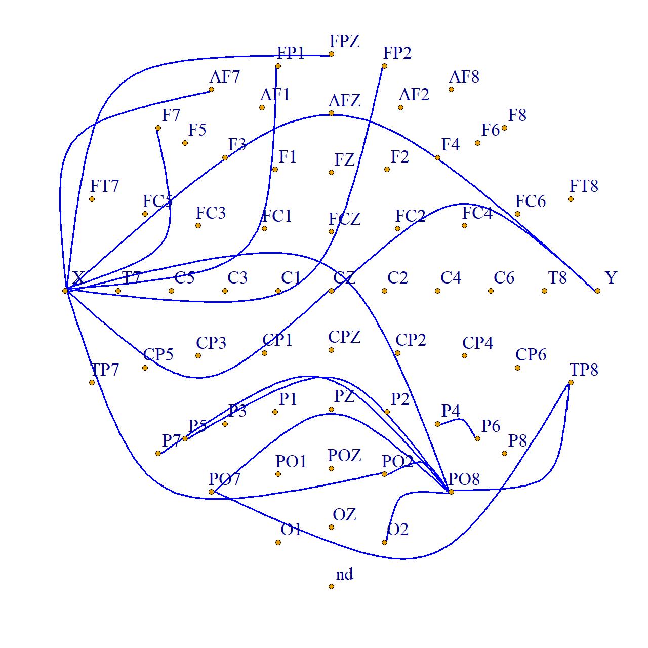
Refer to caption
Figure 6: Estimated differential graph for EEG data. The anterior region is the top of the figure and the posterior region is the bottom of the figure.

We give two specific observations. First, edges are generally between nodes located in the same region—either the anterior region or the posterior region—and there is no edge that crosses between regions. This observation is consistent with the result in Qiao et al. 2019 where there are no connections between the anterior and posterior regions for both groups. We also note that electrode X, lying in the middle left region, has a high degree in the estimated differential graph. Although there is no direct connection between the anterior and posterior regions, this region may play a role in helping the two parts communicate and may be greatly affected by AUD. Similarly, P08 in the anterior region also has a high degree and is connected to other nodes in the anterior region, which may indicate that this region can be an information exchange center for the anterior regions, which, at the same time, may be heavily affected by AUD.

7 Discussion

We proposed a method to directly estimate the differential graph for functional graphical models. In certain settings, direct estimation allows the differential graph to be recovered consistently, even if each underlying graph cannot be consistently recovered. Experiments with simulated data also show that preserving the functional nature of the data rather than treating the data as multivariate scalars can also result in better estimation of the differential graph.

A key step in the procedure is to first represent the functions with an MM-dimensional basis using FPCA. Definition 4 ensures that there exists some MM large enough so that the signal, ν1​(M)\nu_{1}(M), is larger than the bias, ν2​(M)\nu_{2}(M), due to the use of a finite-dimensional representation. Intuitively, τ=ν1​(M)−ν2​(M)\tau=\nu_{1}(M)-\nu_{2}(M) is tied to the eigenvalue decay rate; however, we defer the derivation of the explicit connection for future work.

We have provided a method for direct estimation of the differential graph, but the development of methods that allow for inference and hypothesis testing in functional differential graphs is a fruitful avenue for future work. In recent years, a number of studies have focused on inference in high-dimensional linear models (Zhang and Zhang 2014; van de Geer et al. 2014; Javanmard and Montanari 2014; Zhao et al. 2014b; Bradic and Kolar 2017; Wang et al. 2021). Subsequently, these approaches were extended for statistical inference of low-dimensional parameters in graphical models (Ren et al. 2015; Wasserman et al. 2014; Janková and van de Geer 2015; Janková and van de Geer 2017; Barber and Kolar 2018; Yu et al. 2016; Yu et al. 2020) and differential graphical models (Xia et al. 2015; Liu 2017; Kim et al. 2021). Future work may extend these results to the functional graph setting. A promising approach would be to extend the inference procedures developed for semi- and non-parametric models (Lu et al. 2020; Dai and Kolar 2021, see, e.g.,).

acknowledgments-disclosure-of-funding.
We thank the associate editor Daniela Witten and reviewers for their helpful feedback which has greatly improved the manuscript. This work is partially supported by the William S. Fishman Faculty Research Fund at the University of Chicago Booth School of Business. This work was completed in part with resources provided by the University of Chicago Research Computing Center.

Appendix A Derivation of Optimization Algorithm

In this section, we derive the key steps for optimization algorithms.

A.1 Optimization Algorithm for FuDGE

We derive closed-form updates for the proximal method stated in (28). In particular, recall that for all 1≤j,l≤p1\leq{j,l}\leq{p}, we have

Δj​lnew=[(‖Aj​lold‖F−λn​η)/‖Aj​lold‖F]+×Aj​lold,\Delta^{\text{new}}_{jl}\;=\;\left[\left(\|A^{\text{old}}_{jl}\|_{F}-\lambda_{n}\eta\right)/\|A^{\text{old}}_{jl}\|_{F}\right]_{+}\times A^{\text{old}}_{jl},

where Aold=Δold−η∇ℒ(Δold)A^{\text{old}}=\Delta^{\text{old}}-\eta\nabla\mathcal{L}(\Delta^{\text{old}}) and x+=max⁡{0,x}x_{+}=\max\{0,x\} represents the positive part of x∈ℝx\in{\mathbb{R}}.

Proof of (28).

Let Aold=Δold−η∇ℒ(Δold)A^{\text{old}}=\Delta^{\text{old}}-\eta\nabla\mathcal{L}(\Delta^{\text{old}}) and let fj​lf_{jl} denote the loss decomposed over each j,lj,l block so that

fj​l​(Δj​l)=12​λn​η​‖Δj​l−Aj​lold‖F2+‖Δj​l‖F{}f_{jl}(\Delta_{jl})\;=\;\frac{1}{2\lambda_{n}\eta}\|\Delta_{jl}-A^{\text{old}}_{jl}\|^{2}_{F}+\|\Delta_{jl}\|_{F} (A.1)

and

Δj​lnew=arg​minΔjl∈ℝM×M⁡fjl​(Δjl).\Delta^{\text{new}}_{jl}\;=\;\argmin_{\Delta_{jl}\in{\mathbb{R}^{M\times{M}}}}f_{jl}(\Delta_{jl}). (A.2)

The loss fj​l​(Δj​l)f_{jl}(\Delta_{jl}) is convex, so the first-order optimality condition implies that:

0∈∂fj​l​(Δj​lnew),{}0\in\partial f_{jl}\left(\Delta^{\text{new}}_{jl}\right), (A.3)

where ∂fj​l​(Δj​l)\partial f_{jl}\left(\Delta_{jl}\right) is the subdifferential of fj​lf_{jl} at Δj​l\Delta_{jl}:

∂fj​l​(Δj​l)=1λn​η​(Δj​l−Aj​lold)+Zj​l,{}\partial f_{jl}(\Delta_{jl})\;=\;\frac{1}{\lambda_{n}\eta}\left(\Delta_{jl}-A^{\text{old}}_{jl}\right)+Z_{jl}, (A.4)

where

Zj​l={Δj​l‖Δj​l‖F if ​Δj​l≠0{Zj​l∈ℝM×M:‖Zj​l‖F≤1} if ​Δj​l=0.{}Z_{jl}\;=\;\begin{cases}\frac{\Delta_{jl}}{\|\Delta_{jl}\|_{F}}\qquad&\text{ if }\Delta_{jl}\neq{0}\\[10.0pt] \left\{Z_{jl}\in{\mathbb{R}^{M\times{M}}}\colon\|Z_{jl}\|_{F}\leq{1}\right\}\qquad&\text{ if }\Delta_{jl}=0.\end{cases} (A.5)

Claim 1 If ‖Aj​lold‖F>λn​η>0\|A^{\text{old}}_{jl}\|_{F}>\lambda_{n}\eta>0, then Δj​lnew≠0\Delta^{\text{new}}_{jl}\neq{0}.

We verify this claim by proving the contrapositive. Suppose Δj​lnew=0\Delta^{\text{new}}_{jl}={0}. Then by (A.3) and (A.5), there exists a Zj​l∈ℝM×MZ_{jl}\in{\mathbb{R}^{M\times{M}}} such that ‖Zj​l‖F≤1\|Z_{jl}\|_{F}\leq{1} and

0=−1λn​η​Aj​lold+Zj​l.0=-\frac{1}{\lambda_{n}\eta}A^{\text{old}}_{jl}+Z_{jl}.

Thus, ‖Aj​lold‖F=‖λn​η⋅Zj​l‖F≤λn​η\|A^{\text{old}}_{jl}\|_{F}=\|\lambda_{n}\eta\cdot Z_{jl}\|_{F}\leq{\lambda_{n}\eta}, so that Claim 1 holds.

Combining Claim 1 with (A.3) and (A.5), for any j,lj,l such that ‖Aj​lold‖F>λn​η\|A^{\text{old}}_{jl}\|_{F}>\lambda_{n}\eta, we have

0=1λn​η​(Δj​lnew−Aj​lold)+Δj​lnew‖Δj​lnew‖F,0=\frac{1}{\lambda_{n}\eta}\left(\Delta^{\text{new}}_{jl}-A^{\text{old}}_{jl}\right)+\frac{\Delta^{\text{new}}_{jl}}{\|\Delta^{\text{new}}_{jl}\|_{F}},

which is solved by

Δj​lnew=‖Aj​lold‖F−λn​η‖Aj​lold‖F​Aj​lold.{}\Delta^{\text{new}}_{jl}=\frac{\|A^{\text{old}}_{jl}\|_{F}-\lambda_{n}\eta}{\|A^{\text{old}}_{jl}\|_{F}}A^{\text{old}}_{jl}. (A.6)

Claim 2 If ‖Aj​lold‖F≤λn​η\|A^{\text{old}}_{jl}\|_{F}\leq\lambda_{n}\eta, then Δj​lnew=0\Delta^{\text{new}}_{jl}=0.

Again, we verify the claim by proving the contrapositive. Suppose Δj​lnew≠0\Delta^{\text{new}}_{jl}\neq 0. Then the first-order optimality implies the updates in (A.6). However, taking the Frobenius norm on both sides of the equation gives ‖Δj​lnew‖F=‖Aj​lold‖F−λn​η\|\Delta^{\text{new}}_{jl}\|_{F}=\|A^{\text{old}}_{jl}\|_{F}-\lambda_{n}\eta, which implies that ‖Aj​lold‖F−λn​η≥0\|A^{\text{old}}_{jl}\|_{F}-\lambda_{n}\eta\geq{0}.

Updates in (28) follow immediately by combining Claim 2 and (A.6). ∎

A.2 Solving the Joint Functional Graphical Lasso

As in Danaher et al. 2014, we use the alternating directions method of multipliers (ADMM) algorithm to solve (44); see Boyd et al. 2011 for a detailed exposition of ADMM.

To solve (44), we first rewrite the problem as:

max{Θ},{Z}{−∑q=1Qnq(logdetΘ(q)−trace(S(q)Θ(q)))+P({Z})},\max_{\{\Theta\},\{Z\}}\left\{-\sum^{Q}_{q=1}n_{q}\left(\log\text{det}\Theta^{(q)}-\text{trace}\left(S^{(q)}\Theta^{(q)}\right)\right)+P(\{Z\})\right\},

subject to Θ(q)≻0\Theta^{(q)}\succ 0 and Z(q)=Θ(q)Z^{(q)}=\Theta^{(q)}, where {Z}={Z(1),Z(2),…,Z(Q)}\{Z\}=\{Z^{(1)},Z^{(2)},\dots,Z^{(Q)}\}. The scaled augmented Lagrangian (Boyd et al. 2011) is given by

Lρ({Θ},{Z},{U})=−∑Qq=1nq(logdetΘ(q)−trace(S(q)Θ(q)))+P({Z})+ρ2∑Qq=1∥Θ(q)−Z(q)+U(q)∥2F,L_{\rho}\left(\{\Theta\},\{Z\},\{U\}\right)=-\sum^{Q}_{q=1}n_{q}\left(\log\text{det}\Theta^{(q)}-\text{trace}\left(S^{(q)}\Theta^{(q)}\right)\right)+P(\{Z\})\\ +\frac{\rho}{2}\sum^{Q}_{q=1}\|\Theta^{(q)}-Z^{(q)}+U^{(q)}\|^{2}_{\text{F}}, (A.7)

where ρ>0\rho>0 is a tuning parameter and {U}={U(1),U(2),…,U(Q)}\{U\}=\{U^{(1)},U^{(2)},\dots,U^{(Q)}\} are dual variables. The ADMM algorithm will then solve (A.7) by iterating the following three steps. At the ii-th iteration, they are as follows:

  1. 1.

    {Θ(i)}←arg​min{Θ}⁡Lρ​({Θ},{Z(i−1)},{U(i−1)})\{\Theta_{(i)}\}\leftarrow\argmin_{\{\Theta\}}L_{\rho}\left(\{\Theta\},\{Z_{(i-1)}\},\{U_{(i-1)}\}\right).

  2. 2.

    {Z(i)}←arg​min{Z}⁡Lρ​({Θ(i)},{Z},{U(i−1)})\{Z_{(i)}\}\leftarrow\argmin_{\{Z\}}L_{\rho}\left(\{\Theta_{(i)}\},\{Z\},\{U_{(i-1)}\}\right).

  3. 3.

    {U(i)}←{U(i−1)}+({Θ(i)}−{Z(i)})\{U_{(i)}\}\leftarrow\{U_{(i-1)}\}+(\{\Theta_{(i)}\}-\{Z_{(i)}\}).

We now give more details on the above three steps.

ADMM algorithm for solving the joint functional graphical lasso problem

Input: {S(q)}q=1Q\{S^{(q)}\}^{Q}_{q=1}, {nq}q=1Q\{n_{q}\}^{Q}_{q=1}, and the penalty term P⁡(⋅)P(\cdot).

Output: {Θ^(q)}q=1Q\{\hat{\Theta}^{(q)}\}^{Q}_{q=1}.

(a) Initialize the variables: Θ(0)(q)=Ip​M\Theta^{(q)}_{(0)}=I_{pM}, U(0)(q)=0p​MU^{(q)}_{(0)}=0_{pM}, and Z(0)(q)=0p​MZ^{(q)}_{(0)}=0_{pM}, q=1,…,Qq=1,\ldots,Q.

(b) Select a scalar ρ>0\rho>0.

(c) For i=1,2,3,…i=1,2,3,\dots until convergence

(i) For q=1,…,Qq=1,\ldots,Q, update Θ(i)(q)\Theta^{(q)}_{(i)} as the minimizer (with respect to Θ(q)\Theta^{(q)}) of

−nq​(log⁡det​Θ(q)−trace​(S(q)​Θ(q)))+ρ2​‖Θ(q)−Z(i−1)(q)+U(i−1)(q)‖F2-n_{q}\left(\log\text{det}\Theta^{(q)}-\text{trace}\left(S^{(q)}\Theta^{(q)}\right)\right)+\frac{\rho}{2}\|\Theta^{(q)}-Z^{(q)}_{(i-1)}+U^{(q)}_{(i-1)}\|^{2}_{\text{F}}

Let V​D​V⊤VDV^{\top} denote the eigendecomposition of S(q)−ρ​Z(i−1)(q)/nq+ρ​U(i−1)(q)/nqS^{(q)}-\rho Z^{(q)}_{(i-1)}/n_{q}+\rho U^{(q)}_{(i-1)}/n_{q}. The solution is given by V​D~​V⊤V\tilde{D}V^{\top}, where D~\tilde{D} is the diagonal matrix with the jj-th diagonal element being

nq2​ρ​(−Dj​j+Dj​j2+4​ρ/nq),\frac{n_{q}}{2\rho}\left(-D_{jj}+\sqrt{D^{2}_{jj}+4\rho/n_{q}}\right),

where Dj​jD_{jj} is the (j,j)(j,j)-th entry of DD.

(ii) Update {Z(i)}\{Z_{(i)}\} as minimizer (with respect to {Z}\{Z\}) of

min{Z}⁡ρ2​∑q=1Q‖Z(q)−A(q)‖F2+P⁡({Z}),\min_{\{Z\}}\frac{\rho}{2}\sum^{Q}_{q=1}\|Z^{(q)}-A^{(q)}\|^{2}_{\text{F}}+P(\{Z\}), (A.8)

where A(q)=Θ(i)(q)+U(i−1)(q)A^{(q)}=\Theta^{(q)}_{(i)}+U^{(q)}_{(i-1)}, q=1,…,Qq=1,\ldots,Q.

(iii) U(i)(q)←U(i−1)(q)+(Θ(i)(q)−Z(i)(q))U^{(q)}_{(i)}\leftarrow U^{(q)}_{(i-1)}+(\Theta^{(q)}_{(i)}-Z^{(q)}_{(i)}), q=1,…,Qq=1,\ldots,Q.

(d) Output Θ^(q)\hat{\Theta}^{(q)} as Θ(i)(q)\Theta^{(q)}_{(i)}, q=1,…,Qq=1,\ldots,Q, from the final round.

There are three things that are worth noting. 1. The key step is to solve (A.8), which depends on the form of penalty term P⁡(⋅)P(\cdot); 2. This algorithm is guaranteed to converge to the global optimum when P⁡(⋅)P(\cdot) is convex (Boyd et al. 2011); 3. The positive-definiteness constraint on {Θ^}\{\hat{\Theta}\} is naturally enforced by step (c) (i).

A.3 Solving (A.8) for different penalty functions

We provide solutions to (A.8) for three problems (GFGL, FFGL, FFGL2) defined by (47), (48), and (49).

A.3.1 Solution to (A.8) for GFGL

Let the solution for

min{Z}⁡ρ2​∑q=1Q‖Z(q)−A(q)‖F2+λ1​∑q=1Q∑j≠l‖Zj​l(q)‖F+λ2​∑j≠l(∑q=1Q‖Zj​l(q)‖F2)1/2\min_{\{Z\}}\frac{\rho}{2}\sum^{Q}_{q=1}\|Z^{(q)}-A^{(q)}\|^{2}_{\text{F}}+\lambda_{1}\sum^{Q}_{q=1}\sum_{j\neq l}\|Z^{(q)}_{jl}\|_{\text{F}}+\lambda_{2}\sum_{j\neq l}\left(\sum^{Q}_{q=1}\|Z^{(q)}_{jl}\|^{2}_{\text{F}}\right)^{1/2} (A.9)

be denoted as {Z^}={Z^(1),Z^(2),…,Z^(Q)}\{\hat{Z}\}=\{\hat{Z}^{(1)},\hat{Z}^{(2)},\dots,\hat{Z}^{(Q)}\}. Let Zj​l(q)Z^{(q)}_{jl}, Z^j​l(q)\hat{Z}^{(q)}_{jl} be the (j,l)(j,l)-th M×MM\times M block of Z(q)Z^{(q)} and Z^(q)\hat{Z}^{(q)}, q=1,…,Qq=1,\ldots,Q. Then, for j=1,…,pj=1,\ldots,p, we have

Z^(q)j​j=A(q)j​j,q=1,…,Q,\hat{Z}^{(q)}_{jj}=A^{(q)}_{jj},\qquad q=1,\ldots,Q, (A.10)

and, for j≠lj\neq l, we have

Z^j​l(q)=(‖Aj​l(q)‖F−λ1/ρ‖Aj​l(q)‖F)+​(1−λ2ρ​∑q=1Q(‖Aj​l(q)‖F−λ1/ρ)+2)+​Aj​l(q),\hat{Z}^{(q)}_{jl}=\left(\frac{\|A^{(q)}_{jl}\|_{\text{F}}-\lambda_{1}/\rho}{\|A^{(q)}_{jl}\|_{\text{F}}}\right)_{+}\left(1-\frac{\lambda_{2}}{\rho\sqrt{\sum^{Q}_{q=1}\left(\|A^{(q)}_{jl}\|_{\text{F}}-\lambda_{1}/\rho\right)^{2}_{+}}}\right)_{+}A^{(q)}_{jl}, (A.11)

where q=1,…,Qq=1,\ldots,Q. Details of the proof of (A.10) and (A.11) are given in Appendix A.4.

A.3.2 Solution to (A.8) for FFGL

For FFGL, there is no simple closed-form solution. When Q=2Q=2, (A.8) becomes

min{Z}⁡ρ2​∑q=12‖Z(q)−A(q)‖F2+λ1​(∑q=12∑j≠l‖Zj​l(q)‖F)+λ2​∑j,l‖Zj​l(1)−Zj​l(2)‖F.\min_{\{Z\}}\;\frac{\rho}{2}\sum^{2}_{q=1}\|Z^{(q)}-A^{(q)}\|^{2}_{\text{F}}+\lambda_{1}\left(\sum^{2}_{q=1}\sum_{j\neq l}\|Z^{(q)}_{jl}\|_{\text{F}}\right)+\lambda_{2}\sum_{j,l}\|Z^{(1)}_{jl}-Z^{(2)}_{jl}\|_{\text{F}}.

For each 1≤j,l≤p1\leq j,l\leq p, we compute Z^j​l(1)\hat{Z}^{(1)}_{jl}, Z^j​l(2)\hat{Z}^{(2)}_{jl} by solving

min{Zj​l(1),Zj​l(2)}⁡12​∑q=12‖Zj​l(q)−Aj​l(q)‖F2+λ1ρ​𝟙j≠l​∑q=12‖Zj​l(q)‖F+λ2ρ​‖Zj​l(1)−Zj​l(2)‖F,\min_{\{Z^{(1)}_{jl},Z^{(2)}_{jl}\}}\;\frac{1}{2}\sum^{2}_{q=1}\|Z^{(q)}_{jl}-A^{(q)}_{jl}\|^{2}_{\text{F}}+\frac{\lambda_{1}}{\rho}\mathbbm{1}_{j\neq l}\sum^{2}_{q=1}\|Z^{(q)}_{jl}\|_{\text{F}}+\frac{\lambda_{2}}{\rho}\|Z^{(1)}_{jl}-Z^{(2)}_{jl}\|_{\text{F}}, (A.12)

where 𝟙j≠l=1\mathbbm{1}_{j\neq l}=1 when j≠lj\neq l and 00 otherwise.

When j=lj=l, by Lemma 19, we have the following closed-form updates for {Z^j​j(1),Z^j​j(2)}\{\hat{Z}^{(1)}_{jj},\hat{Z}^{(2)}_{jj}\}, j=1,…,pj=1,\ldots,p. If ‖Aj​j(1)−Aj​j(2)‖F≤2​λ2/ρ\|A^{(1)}_{jj}-A^{(2)}_{jj}\|_{\text{F}}\leq 2\lambda_{2}/\rho, then

Z^j​j(1)=Z^j​j(2)=12​(Aj​j(1)+Aj​j(2)).\hat{Z}^{(1)}_{jj}=\hat{Z}^{(2)}_{jj}=\frac{1}{2}\left(A^{(1)}_{jj}+A^{(2)}_{jj}\right).

If ‖Aj​j(1)−Aj​j(2)‖F>2​λ2/ρ\|A^{(1)}_{jj}-A^{(2)}_{jj}\|_{\text{F}}>2\lambda_{2}/\rho, then

Z^j​j(1)\displaystyle\hat{Z}^{(1)}_{jj} =Aj​j(1)−λ2/ρ‖Aj​j(1)−Aj​j(2)‖F​(Aj​j(1)−Aj​j(2)),\displaystyle=A^{(1)}_{jj}-\frac{\lambda_{2}/\rho}{\|A^{(1)}_{jj}-A^{(2)}_{jj}\|_{\text{F}}}\left(A^{(1)}_{jj}-A^{(2)}_{jj}\right),
Z^j​j(2)\displaystyle\hat{Z}^{(2)}_{jj} =Aj​j(2)+λ2/ρ‖Aj​j(1)−Aj​j(2)‖F​(Aj​j(1)−Aj​j(2)).\displaystyle=A^{(2)}_{jj}+\frac{\lambda_{2}/\rho}{\|A^{(1)}_{jj}-A^{(2)}_{jj}\|_{\text{F}}}\left(A^{(1)}_{jj}-A^{(2)}_{jj}\right).

For j≠lj\neq l, we get {Z^j​l(1),Z^j​l(2)}\{\hat{Z}^{(1)}_{jl},\hat{Z}^{(2)}_{jl}\} using the ADMM algorithm again. We construct the scaled augmented Lagrangian as:

L′ρ′​({W},{R},{V})=12​∑q=12‖W(q)−B(q)‖F+λ1ρ​∑q=12‖W(q)‖F+λ2ρ​‖R(1)−R(2)‖F+ρ′2​∑q=12‖W(q)−R(q)+V(q)‖F2,{L^{\prime}}_{\rho^{\prime}}\left(\{W\},\{R\},\{V\}\right)=\frac{1}{2}\sum^{2}_{q=1}\|W^{(q)}-B^{(q)}\|_{\text{F}}+\frac{\lambda_{1}}{\rho}\sum^{2}_{q=1}\|W^{(q)}\|_{\text{F}}\\ +\frac{\lambda_{2}}{\rho}\|R^{(1)}-R^{(2)}\|_{\text{F}}+\frac{\rho^{\prime}}{2}\sum^{2}_{q=1}\|W^{(q)}-R^{(q)}+V^{(q)}\|^{2}_{\text{F}},

where ρ′>0\rho^{\prime}>0 is a tuning parameter, B(q)=Aj​l(q)B^{(q)}=A^{(q)}_{jl}, q=1,2q=1,2, and W(q),R(q),V(q)∈ℝM×MW^{(q)},R^{(q)},V^{(q)}\in\mathbb{R}^{M\times M}, q=1,2q=1,2. {W}={W(1),W(2)}\{W\}=\{W^{(1)},W^{(2)}\}, {R}={R(1),R(2)}\{R\}=\{R^{(1)},R^{(2)}\}, and {V}={V(1),V(2)}\{V\}=\{V^{(1)},V^{(2)}\}. The detailed ADMM algorithm is described as below:

ADMM algorithm for solving (A.12) for j≠lj\neq l

Input: Aj​l(q)A^{(q)}_{jl}, q=1,2q=1,2; λ1,λ2≥0\lambda_{1},\lambda_{2}\geq 0.

Output: {Z^j​l(1),Z^j​l(2)}\{\hat{Z}^{(1)}_{jl},\hat{Z}^{(2)}_{jl}\}.

(a) Initialize the variables: W(0)(q)=IMW^{(q)}_{(0)}=I_{M}, R(0)(q)=0MR^{(q)}_{(0)}=0_{M}, V(0)(q)=0MV^{(q)}_{(0)}=0_{M}, B(q)=Aj​l(q)B^{(q)}=A^{(q)}_{jl}, q=1,2q=1,2.

(b) Select a scalar ρ′>0\rho^{\prime}>0.

(c) For i=1,2,3,…i=1,2,3,\dots until convergence

(i) {W(i)}←arg​min{W}⁡L′ρ′​({W},{R(i−1)},{V(i−1)})\{W_{(i)}\}\leftarrow\argmin_{\{W\}}{L^{\prime}}_{\rho^{\prime}}\left(\{W\},\{R_{(i-1)}\},\{V_{(i-1)}\}\right).

This is equivalent to

{W(i)}←arg​min{W}⁡12​∑q=12‖W(q)−C(q)‖F2+λ1ρ⁡(1+ρ′)​∑q=12‖W(q)‖F,\{W_{(i)}\}\leftarrow\argmin_{\{W\}}\frac{1}{2}\sum^{2}_{q=1}\|W^{(q)}-C^{(q)}\|^{2}_{\text{F}}+\frac{\lambda_{1}}{\rho(1+\rho^{\prime})}\sum^{2}_{q=1}\|W^{(q)}\|_{\text{F}},

where

C(q)=11+ρ′​[B(q)+ρ′​(R(i−1)(q)−V(i−1)(q))].C^{(q)}=\frac{1}{1+\rho^{\prime}}\left[B^{(q)}+\rho^{\prime}\left(R^{(q)}_{(i-1)}-V^{(q)}_{(i-1)}\right)\right].

Similar to (27), we have

W(i)(q)←(‖C(q)‖F−λ1/(ρ⁡(1+ρ′))‖C(q)‖F)+⋅C(q),q=1,2.W^{(q)}_{(i)}\leftarrow\left(\frac{\|C^{(q)}\|_{\text{F}}-\lambda_{1}/(\rho(1+\rho^{\prime}))}{\|C^{(q)}\|_{\text{F}}}\right)_{+}\cdot C^{(q)},\qquad q=1,2.

(ii) {R(i)}←arg​min{R}⁡L′ρ′​({W(i)},{R},{V(i−1)})\{R_{(i)}\}\leftarrow\argmin_{\{R\}}{L^{\prime}}_{\rho^{\prime}}\left(\{W_{(i)}\},\{R\},\{V_{(i-1)}\}\right).

This is equivalent to

{R(i)}←arg​min{R}⁡12​∑q=12‖R(q)−D(q)‖F2+λ2ρ​ρ′​‖R(1)−R(2)‖F,\{R_{(i)}\}\leftarrow\argmin_{\{R\}}\frac{1}{2}\sum^{2}_{q=1}\|R^{(q)}-D^{(q)}\|^{2}_{\text{F}}+\frac{\lambda_{2}}{\rho\rho^{\prime}}\|R^{(1)}-R^{(2)}\|_{\text{F}},

where D(q)=W(i)(q)+V(i−1)(q)D^{(q)}=W^{(q)}_{(i)}+V^{(q)}_{(i-1)}. By Lemma 19, if ‖D(1)−D(2)‖F≤2​λ2/(ρ​ρ′)\|D^{(1)}-D^{(2)}\|_{\text{F}}\leq 2\lambda_{2}/(\rho\rho^{\prime}), then

R(i)(1)=R(i)(2)←12​(D(1)+D(2)),R^{(1)}_{(i)}=R^{(2)}_{(i)}\leftarrow\frac{1}{2}\left(D^{(1)}+D^{(2)}\right),

and if ‖D(1)−D(2)‖F>2​λ2/(ρ​ρ′)\|D^{(1)}-D^{(2)}\|_{\text{F}}>2\lambda_{2}/(\rho\rho^{\prime}), then

R(1)←D(1)−λ2/(ρ​ρ′)‖D(1)−D(2)‖F​(D(1)−D(2)),\displaystyle R^{(1)}\leftarrow D^{(1)}-\frac{\lambda_{2}/(\rho\rho^{\prime})}{\|D^{(1)}-D^{(2)}\|_{\text{F}}}\left(D^{(1)}-D^{(2)}\right),
R(2)←D(2)+λ2/(ρ​ρ′)‖D(1)−D(2)‖F​(D(1)−D(2)).\displaystyle R^{(2)}\leftarrow D^{(2)}+\frac{\lambda_{2}/(\rho\rho^{\prime})}{\|D^{(1)}-D^{(2)}\|_{\text{F}}}\left(D^{(1)}-D^{(2)}\right).

(iii) V(i)(q)←V(i−1)(q)+W(i)(q)−R(i)(q)V^{(q)}_{(i)}\leftarrow V^{(q)}_{(i-1)}+W^{(q)}_{(i)}-R^{(q)}_{(i)}, q=1,2q=1,2.

(d) Output {Z^j​l(1),Z^j​l(2)}\{\hat{Z}^{(1)}_{jl},\hat{Z}^{(2)}_{jl}\} as {W(i)(1),W(i)(2)}\{W^{(1)}_{(i)},W^{(2)}_{(i)}\} from the final round.

A.3.3 Solution to (A.8) for FFGL2

For FFGL2, there is also no closed-form solution. Similarly to Section A.3.2, we compute a closed-form solution for {Z^j​j(1),Z^j​j(2)}\{\hat{Z}^{(1)}_{jj},\hat{Z}^{(2)}_{jj}\}, j=1,…,pj=1,\ldots,p, and use an ADMM algorithm to compute {Z^j​l(1),Z^j​l(2)}\{\hat{Z}^{(1)}_{jl},\hat{Z}^{(2)}_{jl}\}, 1≤j≠l≤p1\leq j\neq l\leq p.

For any 1≤j,l≤p1\leq j,l\leq p, we solve:

min{Zj​l(1),Zj​l(2)}⁡12​∑q=12‖Zj​l(q)−Aj​l(q)‖F2+λ1ρ​𝟙j≠l​∑q=12‖Zj​l(q)‖F+λ2ρ​∑1≤a,b≤M|Zj​l,a​b(1)−Zj​l,a​b(2)|,\min_{\{Z^{(1)}_{jl},Z^{(2)}_{jl}\}}\;\frac{1}{2}\sum^{2}_{q=1}\|Z^{(q)}_{jl}-A^{(q)}_{jl}\|^{2}_{\text{F}}+\frac{\lambda_{1}}{\rho}\mathbbm{1}_{j\neq l}\sum^{2}_{q=1}\|Z^{(q)}_{jl}\|_{\text{F}}+\frac{\lambda_{2}}{\rho}\sum_{1\leq a,b\leq M}|Z^{(1)}_{jl,ab}-Z^{(2)}_{jl,ab}|, (A.13)

where 𝟙j≠l=1\mathbbm{1}_{j\neq l}=1 when j≠lj\neq l and 00 otherwise.

By Lemma 19, when j=lj=l we have

(Z^j​j,a​b(1),Z^j​j,a​b(2))\displaystyle\left(\hat{Z}^{(1)}_{jj,ab},\hat{Z}^{(2)}_{jj,ab}\right)
={(Aj​l,a​b(1)−λ2/ρ,Aj​l,a​b(2)+λ2/ρ)if​Aj​l,a​b(1)>Aj​l,a​b(2)+2​λ2/ρ(Aj​l,a​b(1)+λ2/ρ,Aj​l,a​b(2)−λ2/ρ)if​Aj​l,a​b(1)<Aj​l,a​b(2)−2​λ2/ρ((Aj​l,a​b(1)+Aj​l,a​b(2))/2,(Aj​l,a​b(1)+Aj​l,a​b(2))/2)if​|Aj​l,a​b(1)−Aj​l,a​b(2)|≤2​λ2/ρ,\displaystyle\quad=\left\{\begin{array}[]{ll}\left(A^{(1)}_{jl,ab}-\lambda_{2}/\rho,A^{(2)}_{jl,ab}+\lambda_{2}/\rho\right)&\text{if}\;A^{(1)}_{jl,ab}>A^{(2)}_{jl,ab}+2\lambda_{2}/\rho\\ \left(A^{(1)}_{jl,ab}+\lambda_{2}/\rho,A^{(2)}_{jl,ab}-\lambda_{2}/\rho\right)&\text{if}\;A^{(1)}_{jl,ab}<A^{(2)}_{jl,ab}-2\lambda_{2}/\rho\\ \left(\left(A^{(1)}_{jl,ab}+A^{(2)}_{jl,ab}\right)/2,\left(A^{(1)}_{jl,ab}+A^{(2)}_{jl,ab}\right)/2\right)&\text{if}\;\left|A^{(1)}_{jl,ab}-A^{(2)}_{jl,ab}\right|\leq 2\lambda_{2}/\rho\end{array}\right.,

where the subscript denotes the (a,b)(a,b)-th entry, 1≤a,b≤M1\leq a,b\leq M and j=1,…,pj=1,\ldots,p.

For j≠lj\neq l, we get {Z^j​l(1),Z^j​l(2)}\{\hat{Z}^{(1)}_{jl},\hat{Z}^{(2)}_{jl}\}, 1≤j≠l≤p1\leq j\neq l\leq p using an ADMM algorithm. Let B(q)=Aj​l(q)B^{(q)}=A^{(q)}_{jl}, q=1,2q=1,2. We first construct the scaled augmented Lagrangian:

L′ρ′​({W},{R},{V})=12​∑q=12‖W(q)−B(q)‖F+λ1ρ​∑q=12‖W(q)‖F+λ2ρ∑a,b|R(1)a,b−R(2)a,b|+ρ′2∑2q=1∥W(q)−R(q)+V(q)∥2F,{L^{\prime}}_{\rho^{\prime}}\left(\{W\},\{R\},\{V\}\right)=\frac{1}{2}\sum^{2}_{q=1}\|W^{(q)}-B^{(q)}\|_{\text{F}}+\frac{\lambda_{1}}{\rho}\sum^{2}_{q=1}\|W^{(q)}\|_{\text{F}}\\ +\frac{\lambda_{2}}{\rho}\sum_{a,b}|R^{(1)}_{a,b}-R^{(2)}_{a,b}|+\frac{\rho^{\prime}}{2}\sum^{2}_{q=1}\|W^{(q)}-R^{(q)}+V^{(q)}\|^{2}_{\text{F}},

where ρ′>0\rho^{\prime}>0 is a tuning parameter, Wq,R(q),V(q)∈ℝM×MW^{q},R^{(q)},V^{(q)}\in\mathbb{R}^{M\times M}, q=1,2q=1,2, {W}={W(1),W(2)}\{W\}=\{W^{(1)},W^{(2)}\}, {R}={R(1),R(2)}\{R\}=\{R^{(1)},R^{(2)}\}, and {V}={V(1),V(2)}\{V\}=\{V^{(1)},V^{(2)}\}. The detailed ADMM algorithm is described below.

ADMM algorithm for solving (A.13) for j≠lj\neq l

Input: Aj​l(q)A^{(q)}_{jl}, q=1,2q=1,2; λ1,λ2≥0\lambda_{1},\lambda_{2}\geq 0.

Output: {Z^j​l(1),Z^j​l(2)}\{\hat{Z}^{(1)}_{jl},\hat{Z}^{(2)}_{jl}\}.

(a) Initialize the variables: W(0)(q)=IMW^{(q)}_{(0)}=I_{M}, R(0)(q)=0MR^{(q)}_{(0)}=0_{M}, V(0)(q)=0MV^{(q)}_{(0)}=0_{M}, B(q)=Aj​l(q)B^{(q)}=A^{(q)}_{jl}, q=1,2q=1,2.

(b) Select a scalar ρ′>0\rho^{\prime}>0.

(c) For i=1,2,3,…i=1,2,3,\dots until convergence

(i) {W(i)}←arg​min{W}.L′ρ′​({W},{R(i−1)},{V(i−1)})\{W_{(i)}\}\leftarrow\argmin_{\{W\}}.{L^{\prime}}_{\rho^{\prime}}\left(\{W\},\{R_{(i-1)}\},\{V_{(i-1)}\}\right)

This is equivalent to

{W(i)}←arg​min{W}⁡12​∑q=12‖W(q)−C(q)‖F2+λ1ρ⁡(1+ρ′)​∑q=12‖W(q)‖F,\{W_{(i)}\}\leftarrow\argmin_{\{W\}}\frac{1}{2}\sum^{2}_{q=1}\|W^{(q)}-C^{(q)}\|^{2}_{\text{F}}+\frac{\lambda_{1}}{\rho(1+\rho^{\prime})}\sum^{2}_{q=1}\|W^{(q)}\|_{\text{F}},

where

C(q)=11+ρ′​[B(q)+ρ′​(R(i−1)(q)−V(i−1)(q))].C^{(q)}=\frac{1}{1+\rho^{\prime}}\left[B^{(q)}+\rho^{\prime}\left(R^{(q)}_{(i-1)}-V^{(q)}_{(i-1)}\right)\right].

Similarly to (27), we have

W(i)(q)←(‖C(q)‖F−λ1/(ρ⁡(1+ρ′))‖C(q)‖F)+⋅C(q),q=1,2.W^{(q)}_{(i)}\leftarrow\left(\frac{\|C^{(q)}\|_{\text{F}}-\lambda_{1}/(\rho(1+\rho^{\prime}))}{\|C^{(q)}\|_{\text{F}}}\right)_{+}\cdot C^{(q)},\qquad q=1,2.

(ii) {R(i)}←arg​min{R}⁡L′ρ′​({W(i)},{R},{V(i−1)})\{R_{(i)}\}\leftarrow\argmin_{\{R\}}{L^{\prime}}_{\rho^{\prime}}\left(\{W_{(i)}\},\{R\},\{V_{(i-1)}\}\right)

This is equivalent to

{R(i)}←arg​min{R}⁡12​∑q=12‖R(q)−D(q)‖F2+λ2ρ​ρ′​∑a,b|Rab(1)−Rab(2)|,\{R_{(i)}\}\leftarrow\argmin_{\{R\}}\frac{1}{2}\sum^{2}_{q=1}\|R^{(q)}-D^{(q)}\|^{2}_{\text{F}}+\frac{\lambda_{2}}{\rho\rho^{\prime}}\sum_{a,b}\left|R^{(1)}_{ab}-R^{(2)}_{ab}\right|,

where D(q)=W(i)(q)+V(i−1)(q)D^{(q)}=W^{(q)}_{(i)}+V^{(q)}_{(i-1)}. Then, by Lemma 19, we have

(R(i),a​b(1),R(i),a​b(2))\displaystyle\left(R^{(1)}_{(i),ab},R^{(2)}_{(i),ab}\right)
={(Da​b(1)−λ2/(ρ​ρ′),Da​b(2)+λ2/(ρ​ρ′))if​Da​b(1)>Da​b(2)+2​λ2/(ρ​ρ′)(Da​b(1)+λ2/(ρ​ρ′),Da​b(2)−λ2/(ρ​ρ′))if​Da​b(1)<Da​b(2)−2​λ2/(ρ​ρ′)((Da​b(1)+Da​b(2))/2,(Da​b(1)+Da​b(2))/2)if​|Da​b(1)−Da​b(1)|≤2​λ2/(ρ​ρ′),\displaystyle\quad=\left\{\begin{array}[]{ll}\left(D^{(1)}_{ab}-\lambda_{2}/(\rho\rho^{\prime}),D^{(2)}_{ab}+\lambda_{2}/(\rho\rho^{\prime})\right)&\text{if}\;D^{(1)}_{ab}>D^{(2)}_{ab}+2\lambda_{2}/(\rho\rho^{\prime})\\ \left(D^{(1)}_{ab}+\lambda_{2}/(\rho\rho^{\prime}),D^{(2)}_{ab}-\lambda_{2}/(\rho\rho^{\prime})\right)&\text{if}\;D^{(1)}_{ab}<D^{(2)}_{ab}-2\lambda_{2}/(\rho\rho^{\prime})\\ \left(\left(D^{(1)}_{ab}+D^{(2)}_{ab}\right)/2,\left(D^{(1)}_{ab}+D^{(2)}_{ab}\right)/2\right)&\text{if}\;\left|D^{(1)}_{ab}-D^{(1)}_{ab}\right|\leq 2\lambda_{2}/(\rho\rho^{\prime})\end{array}\right.,

where the subscript denotes the (a,b)(a,b)-th entry, 1≤a,b≤M1\leq a,b\leq M and 1≤j,l≤p1\leq j,l\leq p.

(iii) V(i)(q)←V(i−1)(q)+W(i)(q)−R(i)(q)V^{(q)}_{(i)}\leftarrow V^{(q)}_{(i-1)}+W^{(q)}_{(i)}-R^{(q)}_{(i)}, q=1,2q=1,2.

(d) Output {Z^j​l(1),Z^j​l(2)}\{\hat{Z}^{(1)}_{jl},\hat{Z}^{(2)}_{jl}\} as {W(i)(1),W(i)(2)}\{W^{(1)}_{(i)},W^{(2)}_{(i)}\} from the final round.

A.4 Derivation of (A.10) and (A.11)

Note that for any 1≤j,l≤p1\leq j,l\leq p, we can obtain Z^j​l(1),Z^j​l(2),…,Z^j​l(Q)\hat{Z}^{(1)}_{jl},\hat{Z}^{(2)}_{jl},\dots,\hat{Z}^{(Q)}_{jl} by solving

arg​minZjl(1),Zjl(2),…,Zjl(Q)⁡ρ2​∑q=1Q‖Zjl(q)−Ajl(q)‖F2+λ1​𝟙j≠l​∑q=1Q‖Zjl(q)‖F+λ2​𝟙j≠l​(∑q=1Q‖Zjl(q)‖F2)1/2,\argmin_{Z^{(1)}_{jl},Z^{(2)}_{jl},\dots,Z^{(Q)}_{jl}}\frac{\rho}{2}\sum^{Q}_{q=1}\|Z^{(q)}_{jl}-A^{(q)}_{jl}\|^{2}_{\text{F}}+\lambda_{1}\mathbbm{1}_{j\neq l}\sum^{Q}_{q=1}\|Z^{(q)}_{jl}\|_{\text{F}}+\lambda_{2}\mathbbm{1}_{j\neq l}\left(\sum^{Q}_{q=1}\|Z^{(q)}_{jl}\|^{2}_{\text{F}}\right)^{1/2}, (A.14)

where 𝟙j≠l=1\mathbbm{1}_{j\neq l}=1 when j≠lj\neq l and 00 otherwise. By (A.14), we have Z^j​j(q)=Aj​j(q)\hat{Z}^{(q)}_{jj}=A^{(q)}_{jj} for any j=1,…,pj=1,\ldots,p and q=1,…,Qq=1,\ldots,Q, which is (A.10). We then prove (A.11). Denote the objective function in (A.14) by L~j​l\tilde{L}_{jl}. Then, for j≠lj\neq l, the subdifferential of L~j​l\tilde{L}_{jl} with respect to Zj​l(q)Z^{(q)}_{jl} is

∂Zj​l(q)L~j​l=ρ⁡(Zj​l(q)−Aj​l(q))+λ1​Gj​l(q)+λ2​Dj​l(q),\partial_{Z^{(q)}_{jl}}\tilde{L}_{jl}=\rho(Z^{(q)}_{jl}-A^{(q)}_{jl})+\lambda_{1}G^{(q)}_{jl}+\lambda_{2}D^{(q)}_{jl},

where

Gj​l(q)={Zj​l(q)‖Zj​l(q)‖Fwhen​Zj​l(q)≠0{Gj​l(q)∈ℝM×M:‖Gj​l(q)‖F≤1}otherwise,G^{(q)}_{jl}=\left\{\begin{array}[]{ll}\frac{Z^{(q)}_{jl}}{\|Z^{(q)}_{jl}\|_{\text{F}}}&\text{when}\;Z^{(q)}_{jl}\neq 0\\ \{G^{(q)}_{jl}\in\mathbb{R}^{M\times M}:\|G^{(q)}_{jl}\|_{\text{F}}\leq 1\}&\text{otherwise}\end{array}\right.,

and

Dj​l(q)={Zj​l(q)(∑q=1Q‖Zj​l(q)‖F2)1/2when​∑q=1Q‖Zj​l(q)‖F2>0{Dj​l(q)∈ℝM×M:∑q=1Q‖Dj​l(q)‖F2≤1}otherwise.D^{(q)}_{jl}=\left\{\begin{array}[]{ll}\frac{Z^{(q)}_{jl}}{\left(\sum^{Q}_{q=1}\|Z^{(q)}_{jl}\|^{2}_{\text{F}}\right)^{1/2}}&\text{when}\;\sum^{Q}_{q=1}\|Z^{(q)}_{jl}\|^{2}_{\text{F}}>0\\ \{D^{(q)}_{jl}\in\mathbb{R}^{M\times M}:\sum^{Q}_{q=1}\|D^{(q)}_{jl}\|^{2}_{\text{F}}\leq 1\}&\text{otherwise}\end{array}\right..

To obtain the optimum, we need

0∈∂Zj​l(q)L~j​l​(Z^j​l(q))0\in\partial_{Z^{(q)}_{jl}}\tilde{L}_{jl}(\hat{Z}^{(q)}_{jl})

for all q=1,…,Qq=1,\ldots,Q. Now we split our discussion into two cases.

(a) Suppose ∑q=1Q‖Z^j​l(q)‖F2=0\sum^{Q}_{q=1}\|\hat{Z}^{(q)}_{jl}\|^{2}_{\text{F}}=0 or equivalently Z^j​l(q)=0\hat{Z}^{(q)}_{jl}=0 for all q=1,…,Qq=1,\ldots,Q.

In this case, there exist Gj​l(q)G^{(q)}_{jl}, where ‖Gj​l(q)‖F≤1\|G^{(q)}_{jl}\|_{\text{F}}\leq 1, q=1,…,Qq=1,\ldots,Q; and also Dj​l(q)D^{(q)}_{jl}, where ∑q=1Q‖Dj​l(q)‖F2≤1\sum^{Q}_{q=1}\|D^{(q)}_{jl}\|^{2}_{\text{F}}\leq 1, such that

0=−ρ⋅A(q)j​l+λ1G(q)j​l+λ2D(q)j​l.0=-\rho\cdot A^{(q)}_{jl}+\lambda_{1}G^{(q)}_{jl}+\lambda_{2}D^{(q)}_{jl}.

This implies that

Dj​l(q)=ρλ2​(Aj​l(q)−λ1ρ​Gj​l(q)).D^{(q)}_{jl}=\frac{\rho}{\lambda_{2}}\left(A^{(q)}_{jl}-\frac{\lambda_{1}}{\rho}G^{(q)}_{jl}\right).

Thus, we have

‖Dj​l(q)‖F\displaystyle\|D^{(q)}_{jl}\|_{\text{F}} =ρλ2​‖Aj​l(q)−λ1ρ​Gj​l(q)‖F≥ρλ2​(‖Aj​l(q)‖F−λ1ρ​‖Gj​l(q)‖F)+\displaystyle=\frac{\rho}{\lambda_{2}}\left\|A^{(q)}_{jl}-\frac{\lambda_{1}}{\rho}G^{(q)}_{jl}\right\|_{\text{F}}\geq\frac{\rho}{\lambda_{2}}\left(\|A^{(q)}_{jl}\|_{\text{F}}-\frac{\lambda_{1}}{\rho}\|G^{(q)}_{jl}\|_{\text{F}}\right)_{+}
≥ρλ2​(‖Aj​l(q)‖F−λ1ρ)+,\displaystyle\geq\frac{\rho}{\lambda_{2}}\left(\|A^{(q)}_{jl}\|_{\text{F}}-\frac{\lambda_{1}}{\rho}\right)_{+},

which implies that

ρ2λ22​∑q=1Q(‖Aj​l(q)‖F−λ1ρ)+2≤∑q=1Q‖Dj​l(q)‖F2≤1.\frac{\rho^{2}}{\lambda^{2}_{2}}\sum^{Q}_{q=1}\left(\|A^{(q)}_{jl}\|_{\text{F}}-\frac{\lambda_{1}}{\rho}\right)^{2}_{+}\leq\sum^{Q}_{q=1}\|D^{(q)}_{jl}\|^{2}_{\text{F}}\leq 1.

Therefore,

∑q=1Q(‖Aj​l(q)‖F−λ1/ρ)+2≤λ2/ρ.\sqrt{\sum^{Q}_{q=1}\left(\|A^{(q)}_{jl}\|_{\text{F}}-\lambda_{1}/\rho\right)^{2}_{+}}\leq\lambda_{2}/\rho. (A.15)

(b) Suppose ∑q=1Q‖Z^j​l(q)‖F2>0\sum^{Q}_{q=1}\|\hat{Z}^{(q)}_{jl}\|^{2}_{\text{F}}>0.

For those qq’s such that Z^j​l(q)=0\hat{Z}^{(q)}_{jl}=0, there exists Gj​l(q)G^{(q)}_{jl}, where ‖Gj​l(q)‖F=1\|G^{(q)}_{jl}\|_{\text{F}}=1, such that

0=−ρ​Aj​l(q)+λ1​Gj​l(q).0=-\rho A^{(q)}_{jl}+\lambda_{1}G^{(q)}_{jl}.

Thus, we have

‖Aj​l(q)‖F=λ1ρ​‖Gj​l(q)‖F≤λ1ρ,\|A^{(q)}_{jl}\|_{\text{F}}=\frac{\lambda_{1}}{\rho}\|G^{(q)}_{jl}\|_{\text{F}}\leq\frac{\lambda_{1}}{\rho},

which implies that

(‖Aj​l(q)‖F−λ1/ρ)+=0.\left(\|A^{(q)}_{jl}\|_{\text{F}}-\lambda_{1}/\rho\right)_{+}=0. (A.16)

On the other hand, for those qq’s such that Z^j​l(q)≠0\hat{Z}^{(q)}_{jl}\neq 0, we have

0=ρ⁡(Z^j​l(q)−Aj​l(q))+λ1​Z^j​l(q)‖Z^j​l(q)‖F+λ2​Z^j​l(q)(∑q=1Q‖Z^j​l(q)‖F2)1/2,0=\rho\left(\hat{Z}^{(q)}_{jl}-A^{(q)}_{jl}\right)+\lambda_{1}\frac{\hat{Z}^{(q)}_{jl}}{\|\hat{Z}^{(q)}_{jl}\|_{\text{F}}}+\lambda_{2}\frac{\hat{Z}^{(q)}_{jl}}{\left(\sum^{Q}_{q=1}\|\hat{Z}^{(q)}_{jl}\|^{2}_{\text{F}}\right)^{1/2}},

which implies that

Aj​l(q)=Z^j​l(q)​(1+λ1ρ​‖Z^j​l(q)‖F+λ2ρ​(∑q=1Q‖Z^j​l(q)‖F2)1/2),A^{(q)}_{jl}=\hat{Z}^{(q)}_{jl}\left(1+\frac{\lambda_{1}}{\rho\|\hat{Z}^{(q)}_{jl}\|_{\text{F}}}+\frac{\lambda_{2}}{\rho\left(\sum^{Q}_{q=1}\|\hat{Z}^{(q)}_{jl}\|^{2}_{\text{F}}\right)^{1/2}}\right), (A.17)

and

‖Aj​l(q)‖F=‖Z^j​l(q)‖F+λ1/ρ+(λ2/ρ)⋅‖Z^j​l(q)‖F(∑q=1Q‖Z^j​l(q)‖F2)1/2.\|A^{(q)}_{jl}\|_{\text{F}}=\|\hat{Z}^{(q)}_{jl}\|_{\text{F}}+\lambda_{1}/\rho+(\lambda_{2}/\rho)\cdot\frac{\|\hat{Z}^{(q)}_{jl}\|_{\text{F}}}{\left(\sum^{Q}_{q=1}\|\hat{Z}^{(q)}_{jl}\|^{2}_{\text{F}}\right)^{1/2}}. (A.18)

By (A.18), we have

(‖Aj​l(q)‖F−λ1/ρ)+>λ2ρ⋅‖Z^j​l(q)‖F∑q=1Q‖Z^j​l(q)‖F2>0.\left(\|A^{(q)}_{jl}\|_{\text{F}}-\lambda_{1}/\rho\right)_{+}>\frac{\lambda_{2}}{\rho}\cdot\frac{\|\hat{Z}^{(q)}_{jl}\|_{\text{F}}}{\sqrt{\sum^{Q}_{q=1}\|\hat{Z}^{(q)}_{jl}\|^{2}_{\text{F}}}}>0. (A.19)

By (A.16) and (A.19), we have

∑q=Q(‖Aj​l(q)‖F−λ1/ρ)+2\displaystyle\sum^{Q}_{q=}\left(\|A^{(q)}_{jl}\|_{\text{F}}-\lambda_{1}/\rho\right)^{2}_{+} =∑q:‖Z^j​l(q)‖F≠0(∥A(q)j​l∥F−λ1/ρ)2+\displaystyle=\sum_{q:\|\hat{Z}^{(q)}_{jl}\|_{\text{F}}\neq 0}\left(\|A^{(q)}_{jl}\|_{\text{F}}-\lambda_{1}/\rho\right)^{2}_{+} (A.20)
>λ22ρ2∑q:‖Z^j​l(q)‖F≠0‖Z^j​l(q)‖F2∑q=1Q‖Z^j​l(q)‖F2\displaystyle>\frac{\lambda^{2}_{2}}{\rho^{2}}\sum_{q:\|\hat{Z}^{(q)}_{jl}\|_{\text{F}}\neq 0}\frac{\|\hat{Z}^{(q)}_{jl}\|^{2}_{\text{F}}}{\sum^{Q}_{q=1}\|\hat{Z}^{(q)}_{jl}\|^{2}_{\text{F}}}
>λ22/ρ2.\displaystyle>\lambda^{2}_{2}/\rho^{2}.

Now we make the following claims.

Claim 1. ∑q=1Q‖Z^j​l(q)‖F2=0⟺∑q=Q(‖Aj​l(q)‖F−λ1/ρ)+2≤λ2/ρ\sum^{Q}_{q=1}\|\hat{Z}^{(q)}_{jl}\|^{2}_{\text{F}}=0\Longleftrightarrow\sqrt{\sum^{Q}_{q=}\left(\|A^{(q)}_{jl}\|_{\text{F}}-\lambda_{1}/\rho\right)^{2}_{+}}\leq\lambda_{2}/\rho.

This claim is easily shown by (A.15) and (A.20).

Claim 2. When ∑q=1Q‖Z^j​l(q)‖F2>0\sum^{Q}_{q=1}\|\hat{Z}^{(q)}_{jl}\|^{2}_{\text{F}}>0, we have ‖Z^j​l(q)‖F=0⟺‖Aj​l(q)‖F≤λ1/ρ\|\hat{Z}^{(q)}_{jl}\|_{\text{F}}=0\Longleftrightarrow\|A^{(q)}_{jl}\|_{\text{F}}\leq\lambda_{1}/\rho.

This claim is easily shown by (A.16) and (A.19).

Claim 3. When ‖Z^j​l(q)‖F≠0\|\hat{Z}^{(q)}_{jl}\|_{\text{F}}\neq 0, then we have

Z^j​l(q)=(‖Aj​l(q)‖F−λ1/ρ‖Aj​l(q)‖F)​(1−λ2ρ​∑q=Q(‖Aj​l(q)‖F−λ1/ρ)+2)​Aj​l(q).\hat{Z}^{(q)}_{jl}=\left(\frac{\|A^{(q)}_{jl}\|_{\text{F}}-\lambda_{1}/\rho}{\|A^{(q)}_{jl}\|_{\text{F}}}\right)\left(1-\frac{\lambda_{2}}{\rho\sqrt{\sum^{Q}_{q=}\left(\|A^{(q)}_{jl}\|_{\text{F}}-\lambda_{1}/\rho\right)^{2}_{+}}}\right)A^{(q)}_{jl}.

To prove this claim, note that by Claim 2 and (A.18), we have

(∥Aj​l(q)∥F−λ1/ρ)+=∥Z^j​l(q)∥F(1+λ2ρ​(∑q=1Q‖Z^j​l(q)‖F2)1/2),q=1,…,Q.\left(\|A^{(q)}_{jl}\|_{\text{F}}-\lambda_{1}/\rho\right)_{+}=\|\hat{Z}^{(q)}_{jl}\|_{\text{F}}\left(1+\frac{\lambda_{2}}{\rho\left(\sum^{Q}_{q=1}\|\hat{Z}^{(q)}_{jl}\|^{2}_{\text{F}}\right)^{1/2}}\right),\qquad q=1,\ldots,Q.

Thus,

∑q=1Q(‖Aj​l(q)‖F−λ1/ρ)+2=∑q=1Q‖Z^j​l(q)‖F2+λ2/ρ,\sqrt{\sum^{Q}_{q=1}\left(\|A^{(q)}_{jl}\|_{\text{F}}-\lambda_{1}/\rho\right)^{2}_{+}}=\sqrt{\sum^{Q}_{q=1}\|\hat{Z}^{(q)}_{jl}\|^{2}_{\text{F}}}+\lambda_{2}/\rho,

which implies that

∑q=1Q‖Z^j​l(q)‖F2=∑q=1Q(‖Aj​l(q)‖F−λ1/ρ)+2−λ2/ρ.\sqrt{\sum^{Q}_{q=1}\|\hat{Z}^{(q)}_{jl}\|^{2}_{\text{F}}}=\sqrt{\sum^{Q}_{q=1}\left(\|A^{(q)}_{jl}\|_{\text{F}}-\lambda_{1}/\rho\right)^{2}_{+}}-\lambda_{2}/\rho.

Thus, by (A.18), we have

‖Z^j​l(q)‖F\displaystyle\|\hat{Z}^{(q)}_{jl}\|_{\text{F}} =‖Aj​l(q)‖F−λ1/ρ1+λ2/ρ∑q′=1Q(‖Aj​l(q′)‖F−λ1/ρ)+2−λ2/ρ\displaystyle=\frac{\|A^{(q)}_{jl}\|_{\text{F}}-\lambda_{1}/\rho}{1+\frac{\lambda_{2}/\rho}{\sqrt{\sum^{Q}_{q^{\prime}=1}\left(\|A^{(q^{\prime})}_{jl}\|_{\text{F}}-\lambda_{1}/\rho\right)^{2}_{+}}-\lambda_{2}/\rho}}
=(1−λ2ρ​∑q′=1Q(‖Aj​l(q′)‖F−λ1/ρ)+2)​(‖Aj​l(q)‖F−λ1/ρ).\displaystyle=\left(1-\frac{\lambda_{2}}{\rho\sqrt{\sum^{Q}_{q^{\prime}=1}\left(\|A^{(q^{\prime})}_{jl}\|_{\text{F}}-\lambda_{1}/\rho\right)^{2}_{+}}}\right)\left(\|A^{(q)}_{jl}\|_{\text{F}}-\lambda_{1}/\rho\right).

Claim 3 follows by combining the above display with (A.17).

Finally, combining Claims 1-3, we obtain (A.11).

Appendix B Main Technical Proofs

We give proofs of the results given in the main text.

B.1 Proof of Lemma 2

We only need to prove that when we use two sets of orthonormal function basis eM​(t)={ejM​(t)}j=1pe^{M}(t)=\{e^{M}_{j}(t)\}^{p}_{j=1} and e~M​(t)={e~jM​(t)}j=1p\tilde{e}^{M}(t)=\{\tilde{e}^{M}_{j}(t)\}^{p}_{j=1} to expand the same subspace 𝕍[p]M\mathbb{V}^{M}_{[p]}, the definition of EΔπE^{\pi}_{\Delta} will not change. Since both ejM​(t)=(ej​1M​(t),ej​2M​(t),…,ej​MM​(t))⊤e^{M}_{j}(t)=(e^{M}_{j1}(t),e^{M}_{j2}(t),\dots,e^{M}_{jM}(t))^{\top} and e~jM​(t)=(e~j​1M​(t),e~j​2M​(t),…,e~j​MM​(t))⊤\tilde{e}^{M}_{j}(t)=(\tilde{e}^{M}_{j1}(t),\tilde{e}^{M}_{j2}(t),\dots,\tilde{e}^{M}_{jM}(t))^{\top} are orthonormal function basis of 𝕍jM\mathbb{V}^{M}_{j}, there must exist an orthonormal matrix Uj∈ℝM×MU_{j}\in\mathbb{R}^{M\times M} satisfying Uj⊤​Uj=Uj​Uj⊤=IMU^{\top}_{j}U_{j}=U_{j}U^{\top}_{j}=I_{M}, such that e~jM​(t)=Uj​ejM​(t)\tilde{e}^{M}_{j}(t)=U_{j}e^{M}_{j}(t). Let ai​jX,Ma^{X,M}_{ij} be the projection score vectors of Xi​j​(t)X_{ij}(t) onto ejM​(t)e^{M}_{j}(t) and a~i​jX,M\tilde{a}^{X,M}_{ij} be the projection score vectors of Xi​j​(t)X_{ij}(t) onto e~jM​(t)\tilde{e}^{M}_{j}(t). Then a~i​jX,M=Uj​ai​jX,M\tilde{a}^{X,M}_{ij}=U_{j}a^{X,M}_{ij}. Denote

U=diag⁡{U1,U2,…,Up}∈ℝp​M×p​M.U={\rm diag}\{U_{1},U_{2},\dots,U_{p}\}\in\mathbb{R}^{pM\times pM}.

We then have

a~iX,M\displaystyle\tilde{a}^{X,M}_{i} =((a~i​1X,M)⊤,(a~i​2X,M)⊤,…,(a~i​pX,M)⊤)⊤\displaystyle=((\tilde{a}^{X,M}_{i1})^{\top},(\tilde{a}^{X,M}_{i2})^{\top},\dots,(\tilde{a}^{X,M}_{ip})^{\top})^{\top}
=((ai​1X,M)⊤​U1⊤,(ai​2X,M)⊤​U2⊤,…,(ai​pX,M)⊤​Up⊤)⊤=U​aiX,M\displaystyle=((a^{X,M}_{i1})^{\top}U^{\top}_{1},(a^{X,M}_{i2})^{\top}U^{\top}_{2},\dots,(a^{X,M}_{ip})^{\top}U^{\top}_{p})^{\top}=Ua^{X,M}_{i}

and

Σ~X,M=Cov⁡(a~X,M)=U​Cov​(a~X,M)​U⊤=U​ΣX,M​U⊤.\tilde{\Sigma}^{X,M}={\rm Cov}\left(\tilde{a}^{X,M}\right)=U{\rm Cov}\left(\tilde{a}^{X,M}\right)U^{\top}=U\Sigma^{X,M}U^{\top}.

Thus

Θ~X,M=(Σ~X,M)−1=U​(ΣX,M)−1​U⊤=U​ΘX,M​U⊤.\tilde{\Theta}^{X,M}=\left(\tilde{\Sigma}^{X,M}\right)^{-1}=U\left(\Sigma^{X,M}\right)^{-1}U^{\top}=U\Theta^{X,M}U^{\top}.

Therefore, Θ~j​lX,M=Uj​Θj​lX,M​Ul⊤\tilde{\Theta}^{X,M}_{jl}=U_{j}\Theta^{X,M}_{jl}U^{\top}_{l} for all j,l∈V2j,l\in V^{2} and, therefore, ‖Θ~j​lX,M‖F=‖Θj​lX,M‖F\|\tilde{\Theta}^{X,M}_{jl}\|_{\text{F}}=\|\Theta^{X,M}_{jl}\|_{\text{F}} for all j,l∈V2j,l\in V^{2}. This implies the final result.

B.2 Proof of Lemma 3

We first show that Xi​j,Yi​j∈Span⁡{ϕj​1,…,ϕj​Mj⋆}X_{ij},Y_{ij}\in{\rm Span}\left\{\phi_{j1},\dots,\phi_{jM^{\star}_{j}}\right\} almost surely. Let

MjX=sup{M∈ℕ+:λj​MX>0}.M^{X}_{j}=\sup\{M\in\mathbb{N}^{+}:\lambda^{X}_{jM}>0\}.

By Karhunen–Loève theorem, we have Xi​j=∑k=1MjX⟨Xi​j,ϕj​kX⟩​ϕj​kXX_{ij}=\sum^{M^{X}_{j}}_{k=1}\langle X_{ij},\phi^{X}_{jk}\rangle\phi^{X}_{jk} almost surely. Thus, we have Xi​j∈Span⁡{ϕj​1X,…,ϕj,MjXX}X_{ij}\in{\rm Span}\left\{\phi^{X}_{j1},\dots,\phi^{X}_{j,M^{X}_{j}}\right\} almost surely. For any 1≤k≤MjX1\leq k\leq M^{X}_{j}, we have that

∫𝒯Kj​j​(s,t)​ϕkX​(s)​ϕkX​(t)​𝑑s​𝑑t≥∫𝒯Kj​jX​(s,t)​ϕkX​(s)​ϕkX​(t)​𝑑s​𝑑t=λj​kX>0,\int_{\mathcal{T}}K_{jj}(s,t)\phi^{X}_{k}(s)\phi^{X}_{k}(t)dsdt\geq\int_{\mathcal{T}}K^{X}_{jj}(s,t)\phi^{X}_{k}(s)\phi^{X}_{k}(t)dsdt=\lambda^{X}_{jk}>0,

which implies that ϕkX∈Span⁡{ϕj​1,…,ϕj​Mj⋆}\phi^{X}_{k}\in{\rm Span}\left\{\phi_{j1},\dots,\phi_{jM^{\star}_{j}}\right\}. Thus, we have Span⁡{ϕj​1X,…,ϕj,MjXX}⊆Span⁡{ϕj​1,…,ϕj​Mj⋆}{\rm Span}\left\{\phi^{X}_{j1},\dots,\phi^{X}_{j,M^{X}_{j}}\right\}\subseteq{\rm Span}\left\{\phi_{j1},\dots,\phi_{jM^{\star}_{j}}\right\} and Xi​j∈Span⁡{ϕj​1,…,ϕj​Mj⋆}X_{ij}\in{\rm Span}\left\{\phi_{j1},\dots,\phi_{jM^{\star}_{j}}\right\} almost surely. Similarly, we have that Yi​j∈Span⁡{ϕj​1,…,ϕj​Mj⋆}Y_{ij}\in{\rm Span}\left\{\phi_{j1},\dots,\phi_{jM^{\star}_{j}}\right\} almost surely.

Next, we show that Mj′=Mj⋆M^{\prime}_{j}=M^{\star}_{j} by contradiction. By the definition of Mj′M^{\prime}_{j}, we have that Mj′≤Mj⋆M^{\prime}_{j}\leq M^{\star}_{j}. If Mj′≠Mj⋆M^{\prime}_{j}\neq M^{\star}_{j}, then we have 𝕍jMj′⊆ℍ\mathbb{V}^{M^{\prime}_{j}}_{j}\subseteq\mathbb{H} such that Mj′<Mj⋆M^{\prime}_{j}<M^{\star}_{j} and Xi​j,Yi​j∈𝕍jMj′X_{ij},Y_{ij}\in\mathbb{V}^{M^{\prime}_{j}}_{j} almost surely. This implies that there exists ϕ∈Span⁡{ϕj​1,…,ϕj​Mj⋆}∖𝕍jMj′\phi\in{\rm Span}\left\{\phi_{j1},\dots,\phi_{jM^{\star}_{j}}\right\}\setminus\mathbb{V}^{M^{\prime}_{j}}_{j} such that

𝔼⁡[(⟨ϕj​k​(t),Xi​j​(t)⟩)2]=0and𝔼⁡[(⟨ϕj​k​(t),Yi​j​(t)⟩)2]=0\displaystyle\mathbb{E}\left[\left(\langle\phi_{jk}(t),X_{ij}(t)\rangle\right)^{2}\right]=0\quad\text{and}\quad\mathbb{E}\left[\left(\langle\phi_{jk}(t),Y_{ij}(t)\rangle\right)^{2}\right]=0
⇒\displaystyle\Rightarrow ∫𝒯Kj​jX​(s,t)​ϕj​k​(s)​ϕj​k​(t)​𝑑s​𝑑t=0and∫𝒯Kj​jY​(s,t)​ϕj​k​(s)​ϕj​k​(t)​𝑑s​𝑑t=0\displaystyle\int_{\mathcal{T}}K^{X}_{jj}(s,t)\phi_{jk}(s)\phi_{jk}(t)dsdt=0\quad\text{and}\quad\int_{\mathcal{T}}K^{Y}_{jj}(s,t)\phi_{jk}(s)\phi_{jk}(t)dsdt=0
⇒\displaystyle\Rightarrow ∫𝒯Kj​j​(s,t)​ϕj​k​(s)​ϕj​k​(t)​𝑑s​𝑑t=0,\displaystyle\int_{\mathcal{T}}K_{jj}(s,t)\phi_{jk}(s)\phi_{jk}(t)dsdt=0,
⇒\displaystyle\Rightarrow λj​k=0,\displaystyle\lambda_{jk}=0,

which contradicts the definition of Mj⋆M^{\star}_{j}. Thus, we must have Mj′=Mj⋆M^{\prime}_{j}=M^{\star}_{j}.

B.3 Proof of Lemma 7

Let U=V\{j,l}U=V\backslash\{j,l\}, and aUX,M=((ajX,M)⊤,j∈U)⊤a^{X,M}_{U}=\left((a^{X,M}_{j})^{\top},j\in U\right)^{\top}. Without loss of generality, assume that ΣX,M\Sigma^{X,M} and ΘX,M\Theta^{X,M} take the following block structure:

ΣX,M=[Σj​jX,MΣj​lX,MΣj​UX,MΣl​jX,MΣl​lX,MΣl​UX,MΣU​jX,MΣU​lX,MΣU​UX,M],ΘX,M=[Θj​jX,MΘj​lX,MΘj​UX,MΘl​jX,MΘl​lX,MΘl​UX,MΘU​jX,MΘU​lX,MΘU​UX,M].\displaystyle\Sigma^{X,M}=\left[\begin{matrix}\Sigma^{X,M}_{jj}&\Sigma^{X,M}_{jl}&\Sigma^{X,M}_{jU}\\ \Sigma^{X,M}_{lj}&\Sigma^{X,M}_{ll}&\Sigma^{X,M}_{lU}\\ \Sigma^{X,M}_{Uj}&\Sigma^{X,M}_{Ul}&\Sigma^{X,M}_{UU}\\ \end{matrix}\right],\quad\Theta^{X,M}=\left[\begin{matrix}\Theta^{X,M}_{jj}&\Theta^{X,M}_{jl}&\Theta^{X,M}_{jU}\\ \Theta^{X,M}_{lj}&\Theta^{X,M}_{ll}&\Theta^{X,M}_{lU}\\ \Theta^{X,M}_{Uj}&\Theta^{X,M}_{Ul}&\Theta^{X,M}_{UU}\\ \end{matrix}\right].

Let PP denote the submatrix:

P=[Θj​jX,MΘj​lX,MΘl​jX,MΘl​lX,M].P=\left[\begin{matrix}\Theta^{X,M}_{jj}&\Theta^{X,M}_{jl}\\ \Theta^{X,M}_{lj}&\Theta^{X,M}_{ll}\end{matrix}\right].

By standard results for the multivariate Gaussian (Johnson and Wichern 2014), we have

Var⁡(ajX,M∣akX,M,k≠j)=Hj​jX,M=(Θj​jX,M)−1,\displaystyle\mathrm{Var}\left(a^{X,M}_{j}\mid a^{X,M}_{k},k\neq j\right)=H^{X,M}_{jj}=(\Theta^{X,M}_{jj})^{-1},
Var⁡([ajX,MalX,M]∣aUX,M)=P−1=[(P−1)11(P−1)12(P−1)21(P−1)22].\displaystyle\mathrm{Var}\left(\left[\begin{matrix}a^{X,M}_{j}\\ a^{X,M}_{l}\end{matrix}\right]\mid a^{X,M}_{U}\right)=P^{-1}=\left[\begin{matrix}(P^{-1})_{11}&(P^{-1})_{12}\\ (P^{-1})_{21}&(P^{-1})_{22}\end{matrix}\right].

Thus, the first statement directly follows from the first equation. To prove the second statement, we only need to note that

Hj​lX,M\displaystyle H^{X,M}_{jl} =Cov⁡(ajX,M,alX,M∣aUX,M)\displaystyle=\mathrm{Cov}\left(a^{X,M}_{j},a^{X,M}_{l}\mid a^{X,M}_{U}\right)
=(P−1)12\displaystyle=(P^{-1})_{12}
=−(Θj​jX,M)−1​Θj​lX,M​(P−1)22\displaystyle=-(\Theta^{X,M}_{jj})^{-1}\Theta^{X,M}_{jl}(P^{-1})_{22}
=−Hj​jX,M​Θj​lX,M​Hl​l\j,X,M,\displaystyle=-H^{X,M}_{jj}\Theta_{jl}^{X,M}H^{\backslash j,X,M}_{ll},

where the second to last equation follows from the 2×22\times 2 block matrix inverse and the last equation follows from the property of multivariate Gaussian. This completes the proof.

B.4 Proof of Theorem 13

We provide the proof of Theorem 13, following the framework introduced in Negahban et al. 2012. We start by introducing some notation.

We use ⊗\otimes to denote the Kronecker product. For Δ∈ℝp​M×p​M\Delta\in\mathbb{R}^{pM\times pM}, let θ=vec⁡(Δ)∈ℝp2​M2\theta=\vect(\Delta)\in{\mathbb{R}^{p^{2}M^{2}}} and θ∗=vec⁡(ΔM)\theta^{*}=\vect({\Delta^{M}}), where ΔM\Delta^{M} is defined in Section 2.2. Let 𝒢={Gt}t=1,…,N𝒢\mathcal{G}=\{G_{t}\}_{t=1,\ldots,N_{\mathcal{G}}} be a set of indices, where N𝒢=p2N_{\mathcal{G}}=p^{2} and Gt⊂{1,2,⋯,p2​M2}G_{t}\subset\{1,2,\cdots,p^{2}M^{2}\} is the set of indices for θ\theta that correspond to the tt-th M×MM\times M submatrix of ΔM\Delta^{M}. Thus, if t=(j−1)​p+lt=(j-1)p+l, then θGt=vec⁡(Δj​l)∈ℝM2\theta_{G_{t}}=\vect{(\Delta_{jl})}\in{\mathbb{R}^{M^{2}}}, where Δj​l\Delta_{jl} is the (j,l)(j,l)-th M×MM\times{M} submatrix of Δ\Delta. Denote the group indices of θ∗\theta^{*} that belong to blocks corresponding to EΔE_{\Delta} as S𝒢⊆{1,2,⋯,N𝒢}S_{\mathcal{G}}\subseteq{\{1,2,\cdots,N_{\mathcal{G}}\}}. Note that we define S𝒢S_{\mathcal{G}} using EΔE_{\Delta} and not EΔME_{\Delta^{M}}. Therefore, as stated in Assumption 2, |S𝒢|=s|S_{\mathcal{G}}|=s. We further define the subspace ℳ\mathcal{M} as

ℳ≔{θ∈ℝp2​M2∣θGt=0​ for all ​t∉S𝒢}.{}\mathcal{M}\coloneqq{\{\theta\in{\mathbb{R}^{p^{2}M^{2}}}\mid\theta_{G_{t}}=0\text{ for all }t\notin{S_{\mathcal{G}}}\}}. (B.1)

Its orthogonal complement with respect to the Euclidean inner product is

ℳ⊥≔{θ∈ℝp2​M2∣θGt=0​ for all ​t∈S𝒢}.\mathcal{M}^{\bot}\coloneqq{\{\theta\in{\mathbb{R}^{p^{2}M^{2}}}\mid\theta_{G_{t}}=0\text{ for all }t\in{S_{\mathcal{G}}}\}}. (B.2)

For a vector θ\theta, let θℳ\theta_{\mathcal{M}} and θℳ⊥\theta_{\mathcal{M}^{\bot}} be the projection of θ\theta on the subspaces ℳ\mathcal{M} and ℳ⊥\mathcal{M}^{\bot}, respectively. Let ⟨⋅,⋅⟩\langle\cdot,\cdot\rangle represent the Euclidean inner product. Let

ℛ⁡(θ)≔∑t=1N𝒢|θGt|2≜|θ|1,2.{}\mathcal{R}(\theta)\coloneqq{\sum_{t=1}^{N_{\mathcal{G}}}|\theta_{G_{t}}|_{2}}\triangleq{|\theta|_{1,2}}. (B.3)

For any v∈ℝp2​M2v\in{\mathbb{R}^{p^{2}M^{2}}}, the dual norm of ℛ\mathcal{R} is given by

ℛ∗​(v)≔supu∈ℝp2​M2\{0}⟨u,v⟩ℛ⁡(u)=supℛ⁡(u)≤1⟨u,v⟩.{}\mathcal{R}^{*}(v)\coloneqq\sup_{u\in{\mathbb{R}^{p^{2}M^{2}}\backslash{\{0\}}}}\frac{\langle{u},{v}\rangle}{\mathcal{R}(u)}=\sup_{\mathcal{R}(u)\leq{1}}\langle{u},{v}\rangle. (B.4)

The subspace compatibility constant of ℳ\mathcal{M} with respect to ℛ\mathcal{R} is defined as

Ψ⁡(ℳ)≔supu∈ℳ\{0}ℛ⁡(u)|u|2.{}\Psi(\mathcal{M})\coloneqq{\sup_{u\in{\mathcal{M}\backslash\{0\}}}}\frac{\mathcal{R}(u)}{|u|_{2}}. (B.5)
Proof.

By Lemma 18 and Assumption 1, we have

|(SY,M⊗SX,M)−(ΣY,M⊗ΣX,M)|∞≤δn2+2​δn​σmax|(S^{Y,M}\otimes{S^{X,M}})-(\Sigma^{Y,M}\otimes{\Sigma^{X,M}})|_{\infty}\leq\delta_{n}^{2}+2\delta_{n}\sigma_{\max} (B.6)

and

|vec⁡(SY,M−SX,M)−vec⁡(ΣY,M−ΣX,M)|∞≤2​δn.|\vect{(S^{Y,M}-S^{X,M})}-\vect{(\Sigma^{Y,M}-\Sigma^{X,M})}|_{\infty}\leq 2\delta_{n}. (B.7)

The problem (23) can be written in the following form:

θ^λn∈arg​minθ∈ℝp2​M2⁡ℒ​(θ)+λn​ℛ​(θ),\hat{\theta}_{\lambda_{n}}\in\argmin_{\theta\in{\mathbb{R}^{p^{2}M^{2}}}}\mathcal{L}(\theta)+\lambda_{n}\mathcal{R}(\theta), (B.8)

where

ℒ⁡(θ)=12​θ⊤​(SY,M⊗SX,M)​θ−θ⊤​vec⁡(SY,M−SX,M).{}\mathcal{L}(\theta)=\frac{1}{2}\theta^{\top}(S^{Y,M}\otimes{S^{X,M}})\theta-\theta^{\top}\vect({S^{Y,M}-S^{X,M}}). (B.9)

Here, we slightly abuse the notation and use ℒ⁡(⋅)\mathcal{L}(\cdot) to denote the function of θ\theta rather than Δ\Delta. The loss ℒ⁡(θ)\mathcal{L}(\theta) is convex and differentiable with respect to θ\theta, and it can easily be verified that ℛ⁡(⋅)\mathcal{R}(\cdot) defines a vector norm. For h∈ℝp2​M2h\in\mathbb{R}^{p^{2}M^{2}}, the error of the first-order Taylor series expansion of ℒ\mathcal{L} is:

δ​ℒ​(h,θ∗)≔ℒ⁡(θ∗+h)−ℒ⁡(θ∗)−⟨∇ℒ​(θ∗),h⟩=12​h⊤​(SY,M⊗SX,M)​h.\displaystyle\delta{\mathcal{L}}(h,\theta^{*})\coloneqq\mathcal{L}(\theta^{*}+h)-\mathcal{L}(\theta^{*})-\langle\nabla\mathcal{L}(\theta^{*}),h\rangle=\frac{1}{2}h^{\top}(S^{Y,M}\otimes{S^{X,M}})h. (B.10)

From (B.9), we see that ∇ℒ​(θ)=(SY,M⊗SX,M)​θ−vec⁡(SY,M−SX,M)\nabla{\mathcal{L}}(\theta)=(S^{Y,M}\otimes{S^{X,M}})\theta-\vect({S^{Y,M}-S^{X,M}}). By Lemma 22, we have

ℛ∗​(∇ℒ​(θ∗))=maxt=1,2,⋯,N𝒢⁡|[(SY,M⊗SX,M)​θ∗−vec⁡(SY,M−SX,M)]Gt|2.{}\mathcal{R}^{*}(\nabla{\mathcal{L}}(\theta^{*}))=\max_{t=1,2,\cdots,N_{\mathcal{G}}}\left|\left[(S^{Y,M}\otimes{S^{X,M}})\theta^{*}-\vect({S^{Y,M}-S^{X,M}})\right]_{G_{t}}\right|_{2}. (B.11)

Now we establish an upper bound for ℛ∗​(∇ℒ​(θ∗))\mathcal{R}^{*}(\nabla{\mathcal{L}}(\theta^{*})). First, note that

(ΣY,M⊗ΣX,M)​θ∗−vec⁡(ΣY,M−ΣX,M)=vec⁡(ΣX,M​ΔM​ΣY,M−(ΣY,M−ΣX,M))=0.(\Sigma^{Y,M}\otimes{\Sigma^{X,M}})\theta^{*}-\vect({\Sigma^{Y,M}-\Sigma^{X,M}})=\vect({\Sigma^{X,M}\Delta^{M}\Sigma^{Y,M}-(\Sigma^{Y,M}-\Sigma^{X,M})})=0.

Letting (⋅)j​l(\cdot)_{jl} denote the (j,l)(j,l)-th submatrix, we have

|[(SY,M⊗SX,M)​θ∗−vec⁡(SY,M−SX,M)]Gt|2\displaystyle\left|\left[(S^{Y,M}\otimes{S^{X,M}})\theta^{*}-\vect({S^{Y,M}-S^{X,M}})\right]_{G_{t}}\right|_{2} (B.12)
=|[(SY,M⊗SX,M−ΣY,M⊗ΣX,M)​θ∗−vec⁡((SY,M−ΣY,M)−(SX,M−ΣX,M))]Gt|2\displaystyle=\left|\left[(S^{Y,M}\otimes{S^{X,M}}-\Sigma^{Y,M}\otimes{\Sigma^{X,M}})\theta^{*}-\vect{((S^{Y,M}-\Sigma^{Y,M})-(S^{X,M}-\Sigma^{X,M}))}\right]_{G_{t}}\right|_{2}
=‖(SX,M​ΔM​SY,M−ΣX,M​ΔM​ΣY,M)j​l−(SY,M−ΣY,M)j​l−(SX,M−ΣX,M)j​l‖F\displaystyle={\|(S^{X,M}\Delta^{M}S^{Y,M}-\Sigma^{X,M}\Delta^{M}\Sigma^{Y,M})_{jl}-(S^{Y,M}-\Sigma^{Y,M})_{jl}-(S^{X,M}-\Sigma^{X,M})_{jl}\|_{F}}
≤‖(SX,M​ΔM​SY,M−ΣX,M​ΔM​ΣY,M)j​l‖F+‖(SY,M−ΣY,M)j​l‖F+‖(SX,M−ΣX,M)j​l‖F.\displaystyle\leq{\|(S^{X,M}\Delta^{M}S^{Y,M}-\Sigma^{X,M}\Delta^{M}\Sigma^{Y,M})_{jl}\|_{F}+\|(S^{Y,M}-\Sigma^{Y,M})_{jl}\|_{F}+\|(S^{X,M}-\Sigma^{X,M})_{jl}\|_{F}}.

For any M×MM\times{M} matrix AA, ‖A‖F≤M​|A|∞\|A\|_{F}\leq{M|A|_{\infty}}, so

|[(SY,M⊗SX,M)​θ∗−vec⁡(SY,M−SX,M)]Gt|2\displaystyle\left|\left[(S^{Y,M}\otimes{S^{X,M}})\theta^{*}-\vect({S^{Y,M}-S^{X,M}})\right]_{G_{t}}\right|_{2}
≤M[|(SX,MΔMSY,M−ΣX,MΔMΣY,M)j​l|∞\displaystyle\leq M\left[\left|(S^{X,M}\Delta^{M}S^{Y,M}-\Sigma^{X,M}\Delta^{M}\Sigma^{Y,M})_{jl}\right|_{\infty}\right.
+|(SY,M−ΣY,M)j​l|∞+|(SX,M−ΣX,M)j​l|∞]\displaystyle\left.+\left|(S^{Y,M}-\Sigma^{Y,M})_{jl}\right|_{\infty}+\left|(S^{X,M}-\Sigma^{X,M})_{jl}\right|_{\infty}\right]
≤M⁡[|SX,M​ΔM​SY,M−ΣX,M​ΔM​ΣY,M|∞+|SY,M−ΣY,M|∞+|​SX,M−ΣX,M|∞].\displaystyle\leq M\left[\left|S^{X,M}\Delta^{M}S^{Y,M}-\Sigma^{X,M}\Delta^{M}\Sigma^{Y,M}\right|_{\infty}+|S^{Y,M}-\Sigma^{Y,M}|_{\infty}+|S^{X,M}-\Sigma^{X,M}|_{\infty}\right].

For any A∈ℝk×kA\in{\mathbb{R}^{k\times{k}}} and v∈ℝkv\in{\mathbb{R}^{k}}, we have |A​v|∞≤|A|∞|​v|1|Av|_{\infty}\leq{|A|_{\infty}|v|_{1}}. Thus, we also have

|SX,M​ΔM​SY,M−ΣX,M​ΔM​ΣY,M|∞\displaystyle|S^{X,M}\Delta^{M}S^{Y,M}-\Sigma^{X,M}\Delta^{M}\Sigma^{Y,M}|_{\infty} =|[(SY,M⊗SX,M)−(ΣX,M⊗ΣY,M)]​vec⁡(ΔM)|∞\displaystyle=|[(S^{Y,M}\otimes{S^{X,M}})-(\Sigma^{X,M}\otimes{\Sigma^{Y,M}})]\vect{(\Delta^{M})}|_{\infty}
≤|(SY,M⊗SX,M)−(ΣX,M⊗ΣY,M)|∞|​vec⁡(ΔM)|1\displaystyle\leq{|(S^{Y,M}\otimes{S^{X,M}})-(\Sigma^{X,M}\otimes{\Sigma^{Y,M}})|_{\infty}}|\vect{(\Delta^{M})}|_{1}
=|(SY,M⊗SX,M)−(ΣX,M⊗ΣY,M)|∞|​ΔM|1.\displaystyle=|(S^{Y,M}\otimes{S^{X,M}})-(\Sigma^{X,M}\otimes{\Sigma^{Y,M}})|_{\infty}|\Delta^{M}|_{1}.

Combining the inequalities gives an upper bound uniform over 𝒢\mathcal{G} (i.e., for all GtG_{t}):

|[(SY,M⊗SX,M)​θ∗−vec⁡(SY,M−SX,M)]Gt|2≤M[|(SY,M⊗SX,M)−(ΣX,M⊗ΣY,M)|∞|ΔM|1+|SY,M−ΣY,M|∞+|SX,M−ΣX,M|∞],\left|\left[(S^{Y,M}\otimes{S^{X,M}})\theta^{*}-\vect({S^{Y,M}-S^{X,M}})\right]_{G_{t}}\right|_{2}\\ \leq M[|(S^{Y,M}\otimes{S^{X,M}})-(\Sigma^{X,M}\otimes{\Sigma^{Y,M}})|_{\infty}|\Delta^{M}|_{1}\\ +|S^{Y,M}-\Sigma^{Y,M}|_{\infty}+|S^{X,M}-\Sigma^{X,M}|_{\infty}],

which implies

ℛ∗​(∇ℒ​(θ∗))\displaystyle\mathcal{R}^{*}\left(\nabla{\mathcal{L}}(\theta^{*})\right) ≤M[|(SY,M⊗SX,M)−(ΣX,M⊗ΣY,M)|∞|ΔM|1\displaystyle\leq M[|(S^{Y,M}\otimes{S^{X,M}})-(\Sigma^{X,M}\otimes{\Sigma^{Y,M}})|_{\infty}|\Delta^{M}|_{1} (B.13)
+|SY,M−ΣY,M|∞+|SX,M−ΣX,M|∞].\displaystyle+|S^{Y,M}-\Sigma^{Y,M}|_{\infty}+|S^{X,M}-\Sigma^{X,M}|_{\infty}].

Assuming |SX,M−ΣX,M|∞≤δn|S^{X,M}-\Sigma^{X,M}|_{\infty}\leq{\delta_{n}} and |SY,M−ΣY,M|∞≤δn|S^{Y,M}-\Sigma^{Y,M}|_{\infty}\leq\delta_{n} implies

ℛ∗​(∇ℒ​(θ∗))≤M⁡[(δn2+2​δn​σmax)​|ΔM|1+2​δn].{}\mathcal{R}^{*}\left(\nabla{\mathcal{L}}(\theta^{*})\right)\leq{M[(\delta_{n}^{2}+2\delta_{n}\sigma_{\max})|\Delta^{M}|_{1}+2\delta_{n}]}. (B.14)

Setting

λn=2​M​[(δn2+2​δn​σmax)​|ΔM|1+2​δn],{}\lambda_{n}=2M\left[\left(\delta_{n}^{2}+2\delta_{n}\sigma_{\max}\right)\left|\Delta^{M}\right|_{1}+2\delta_{n}\right], (B.15)

then implies that λn≥2​ℛ∗​(∇ℒ​(θ∗))\lambda_{n}\geq{2\mathcal{R}^{*}\left(\nabla{\mathcal{L}}(\theta^{*})\right)}. Thus, invoking Lemma 1 in Negahban et al. 2012, h=θ^λn−θ∗h=\hat{\theta}_{\lambda_{n}}-\theta^{*} must satisfy

ℛ⁡(hℳ⊥)≤3​ℛ​(hℳ)+4​ℛ​(θℳ⊥∗),{}\mathcal{R}(h_{\mathcal{M}^{\bot}})\leq{3\mathcal{R}(h_{\mathcal{M}})}+4\mathcal{R}(\theta^{*}_{\mathcal{M}^{\bot}}), (B.16)

where ℳ\mathcal{M} is defined in (B.1). Equivalently,

|hℳ⊥|1,2≤3​|hℳ|1,2+4|​θℳ⊥∗|1,2.{}|h_{\mathcal{M}^{\bot}}|_{1,2}\leq{3|h_{\mathcal{M}}|_{1,2}}+4|\theta^{*}_{\mathcal{M}^{\bot}}|_{1,2}. (B.17)

By the definition of ν2\nu_{2}, we have

|θℳ⊥∗|1,2=∑t∉𝒮𝒢|θGt∗|2≤(p⁡(p+1)/2−s)​ν2≤p2​ν2.{}|\theta^{*}_{\mathcal{M}^{\bot}}|_{1,2}=\sum_{t\notin{\mathcal{S}_{\mathcal{G}}}}|\theta^{*}_{G_{t}}|_{2}\leq\left(p(p+1)/2-s\right)\nu_{2}\leq p^{2}\nu_{2}. (B.18)

Next, we show that δ​ℒ​(h,θ∗)\delta\mathcal{L}(h,\theta^{*}), as defined in (B.10), satisfies the Restricted Strong Convexity property: δ​ℒ​(h,θ∗)≥κℒ​|h|22−ωℒ2​(θ∗)\delta\mathcal{L}(h,\theta^{*})\geq{\kappa_{\mathcal{L}}|h|^{2}_{2}}-\omega^{2}_{\mathcal{L}}\left(\theta^{*}\right) whenever hh satisfies (B.17). We have

θ⊤​(SY,M⊗SX,M)​θ\displaystyle\theta^{\top}(S^{Y,M}\otimes{S^{X,M}})\theta =θ⊤​(ΣY,M⊗ΣX,M)​θ+θ⊤​(SY,M⊗SX,M−ΣY,M⊗ΣX,M)​θ\displaystyle=\theta^{\top}(\Sigma^{Y,M}\otimes{\Sigma^{X,M}})\theta+\theta^{\top}(S^{Y,M}\otimes{S^{X,M}}-\Sigma^{Y,M}\otimes{\Sigma^{X,M}})\theta
≥θ⊤​(ΣY,M⊗ΣX,M)​θ−|θ⊤​(SY,M⊗SX,M−ΣY,M⊗ΣX,M)​θ|\displaystyle\geq{\theta^{\top}(\Sigma^{Y,M}\otimes{\Sigma^{X,M}})\theta-|\theta^{\top}(S^{Y,M}\otimes{S^{X,M}}-\Sigma^{Y,M}\otimes{\Sigma^{X,M}})\theta|}
≥λmin∗​|θ|22−M2​|SY,M⊗SX,M−ΣY,M⊗ΣX,M|∞|​θ|1,22,\displaystyle\geq{\lambda^{*}_{\min}}|\theta|^{2}_{2}-M^{2}|S^{Y,M}\otimes{S^{X,M}}-\Sigma^{Y,M}\otimes{\Sigma^{X,M}}|_{\infty}|\theta|^{2}_{1,2},

where the last inequality follows from Lemma 20 and λmin∗=λmin​(ΣX,M)×λmin​(ΣY,M)=λmin​(ΣY,M⊗ΣX,M)>0\lambda^{*}_{\min}=\lambda_{\min}(\Sigma^{X,M})\times{\lambda_{\min}(\Sigma^{Y,M})}=\lambda_{\min}(\Sigma^{Y,M}\otimes{\Sigma^{X,M}})>0. Thus,

δ​ℒ​(h,θ∗)\displaystyle\delta\mathcal{L}(h,\theta^{*}) =12​h⊤​(SY,M⊗SX,M)​h\displaystyle=\frac{1}{2}h^{\top}(S^{Y,M}\otimes{S^{X,M}})h
≥12​λmin∗​|h|22−12​M2​|SY,M⊗SX,M−ΣY,M⊗ΣX,M|∞|​h|1,22.\displaystyle\geq{\frac{1}{2}\lambda^{*}_{\min}}|h|^{2}_{2}-\frac{1}{2}M^{2}|S^{Y,M}\otimes{S^{X,M}}-\Sigma^{Y,M}\otimes{\Sigma^{X,M}}|_{\infty}|h|^{2}_{1,2}.

By Lemma 21 and (B.17), we have

|h|1,22\displaystyle|h|^{2}_{1,2} =(|hℳ|1,2+|​hℳ⊥|1,2)2≤16​(|hℳ|1,2+|​θℳ⊥∗|1,2)2\displaystyle=(|h_{\mathcal{M}}|_{1,2}+|h_{\mathcal{M}^{\bot}}|_{1,2})^{2}\leq 16({|h_{\mathcal{M}}|_{1,2}}+|\theta^{*}_{\mathcal{M}^{\bot}}|_{1,2})^{2}
≤16​(s​|h|2+p2​ν2)2≤32​s​|h|22+32​p4​ν22.\displaystyle\leq 16(\sqrt{s}|h|_{2}+p^{2}\nu_{2})^{2}\leq 32s|h|^{2}_{2}+32p^{4}\nu_{2}^{2}.

Combining with the above equation, we get

δ​ℒ​(h,θ∗)\displaystyle\delta\mathcal{L}(h,\theta^{*}) ≥[12​λmin∗−16​M2​s​|SY,M⊗SX,M−ΣY,M⊗ΣX,M|∞]​|h|22\displaystyle\geq{\left[\frac{1}{2}\lambda^{*}_{\min}-16M^{2}s|S^{Y,M}\otimes{S^{X,M}}-\Sigma^{Y,M}\otimes{\Sigma^{X,M}}|_{\infty}\right]}|h|^{2}_{2} (B.19)
−16​M2​p4​ν22​|SY,M⊗SX,M−ΣY,M⊗ΣX,M|∞\displaystyle-16M^{2}p^{4}\nu_{2}^{2}|S^{Y,M}\otimes{S^{X,M}}-\Sigma^{Y,M}\otimes{\Sigma^{X,M}}|_{\infty}
≥[12​λmin∗−8​M2​s​(δn2+2​δn2​σmax)]​|h|22\displaystyle\geq\left[\frac{1}{2}\lambda^{*}_{\min}-8M^{2}s\left(\delta^{2}_{n}+2\delta^{2}_{n}\sigma_{\max}\right)\right]|h|^{2}_{2}
−16​M2​p4​ν22​(δn2+2​δn​σmax).\displaystyle-16M^{2}p^{4}\nu_{2}^{2}\left(\delta^{2}_{n}+2\delta_{n}\sigma_{\max}\right).

Thus, appealing to (B.6), the Restricted Strong Convexity property holds with

κℒ\displaystyle\kappa_{\mathcal{L}} =12​λmin∗−8​M2​s​(δ2+2​δn​σmax),\displaystyle=\;\frac{1}{2}\lambda^{*}_{\min}-8M^{2}s\left(\delta^{2}+2\delta_{n}\sigma_{\max}\right), (B.20)
ωℒ\displaystyle\omega_{\mathcal{L}} = 4​M​p2​ν2​δn2+2​δn​σmax.\displaystyle=\;4Mp^{2}\nu_{2}\sqrt{\delta_{n}^{2}+2\delta_{n}\sigma_{\max}}.

When δn<14​λmin∗+16​M2​s​(σmax)2M2​s−σmax\delta_{n}<\frac{1}{4}\sqrt{\frac{\lambda^{*}_{\min}+16M^{2}s(\sigma_{\max})^{2}}{M^{2}s}}-\sigma_{\max} as we assumed in the theorem, then κℒ>0\kappa_{\mathcal{L}}>0. By Theorem 1 of Negahban et al. 2012 and Lemma 21, letting

λn=2​M​[(δn2+2​δn​σmax)​|ΔM|1+2​δn],\lambda_{n}=2M\left[\left(\delta_{n}^{2}+2\delta_{n}\sigma_{\max}\right)|\Delta^{M}|_{1}+2\delta_{n}\right],

as in (B.15), ensures that

‖Δ^M−ΔM‖F2\displaystyle\|\hat{\Delta}^{M}-\Delta^{M}\|^{2}_{F} =|θ^λn−θ∗|22\displaystyle=|\hat{\theta}_{\lambda_{n}}-\theta^{*}|^{2}_{2} (B.21)
≤9​λn2κℒ2​Ψ2​(ℳ)+λnκℒ​(2​ωℒ2+4​ℛ​(θℳ⊥∗))\displaystyle\leq{9\frac{\lambda^{2}_{n}}{\kappa^{2}_{\mathcal{L}}}}\Psi^{2}(\mathcal{M})+\frac{\lambda_{n}}{\kappa_{\mathcal{L}}}\left(2\omega^{2}_{\mathcal{L}}+4\mathcal{R}(\theta^{*}_{\mathcal{M}^{\bot}})\right)
=9​λn2​sκℒ2+2​λnκℒ​(ωℒ2+2​p2​ν2)\displaystyle=\frac{9\lambda^{2}_{n}s}{\kappa^{2}_{\mathcal{L}}}+\frac{2\lambda_{n}}{\kappa_{\mathcal{L}}}(\omega^{2}_{\mathcal{L}}+2p^{2}\nu_{2})
=Γn2.\displaystyle=\Gamma^{2}_{n}.

We then prove that E^Δ=EΔ\hat{E}_{\Delta}=E_{\Delta}. Recall that we have assumed that 0<Γn<τ/2=(ν1−ν2)/20<\Gamma_{n}<\tau/2=(\nu_{1}-\nu_{2})/2 and ν2+Γn≤ϵn<ν1−Γn\nu_{2}+\Gamma_{n}\leq\epsilon_{n}<\nu_{1}-\Gamma_{n}. Note that we have ‖Δ^j​lM−Δj​lM‖F≤‖Δ^M−ΔM‖F≤Γn\|\hat{\Delta}^{M}_{jl}-\Delta^{M}_{jl}\|_{F}\leq{\|\hat{\Delta}^{M}-\Delta^{M}\|_{F}}\leq\Gamma_{n} for any (j,l)∈V2(j,l)\in{V^{2}}. Recall that

EΔ={(j,l)∈V2:j≠l,Dj​l>0}.{}E_{\Delta}\;=\;\{(j,l)\in{V^{2}}:\;j\neq{l},D_{jl}>0\}. (B.22)

First, we prove that EΔ⊆E^ΔE_{\Delta}\subseteq{\hat{E}_{{\Delta}}}. For any (j,l)∈EΔ(j,l)\in{E_{\Delta}}, by the definition of ν1\nu_{1} in Section 4.1, we have

‖Δ^j​lM‖F\displaystyle\|\hat{\Delta}^{M}_{jl}\|_{F} ≥‖Δj​lM‖F−‖Δ^j​lM−Δj​lM‖F\displaystyle\geq{\|\Delta^{M}_{jl}\|_{F}-\|\hat{\Delta}_{jl}^{M}-\Delta^{M}_{jl}\|_{F}}
≥ν1−Γn\displaystyle\geq\nu_{1}-\Gamma_{n}
>ϵn.\displaystyle>\epsilon_{n}.

The last inequality holds because we have assumed that ϵn<ν1−Γn\epsilon_{n}<\nu_{1}-\Gamma_{n}. Thus, by the definition of E^Δ\hat{E}_{{\Delta}} in (26), we have (j,l)∈E^Δ(j,l)\in{\hat{E}_{{\Delta}}}, which further implies that EΔ⊆E^ΔE_{\Delta}\subseteq{\hat{E}_{{\Delta}}}.

We then show E^Δ⊆EΔ\hat{E}_{{\Delta}}\subseteq{E_{\Delta}}. Let E^Δc\hat{E}^{c}_{{\Delta}} and EΔcE^{c}_{\Delta} denote the complement of E^Δ\hat{E}_{{\Delta}} and EΔE_{\Delta}. For any (j,l)∈EΔc(j,l)\in{E^{c}_{\Delta}}, which also means that (l,j)∈EΔc(l,j)\in{E^{c}_{\Delta}}, by the definition of ν2\nu_{2}, we have that

‖Δ^j​lM‖F\displaystyle\|\hat{\Delta}^{M}_{jl}\|_{F} ≤‖Δj​lM‖F+‖Δ^j​lM−Δj​lM‖F\displaystyle\leq{\|\Delta^{M}_{jl}\|_{F}+\|\hat{\Delta}_{jl}^{M}-\Delta^{M}_{jl}\|_{F}}
≤ν2+Γn\displaystyle\leq\nu_{2}+\Gamma_{n}
≤ϵn.\displaystyle\leq\epsilon_{n}.

Again, the last inequality is true because we have assumed ϵn≥ν2+Γn\epsilon_{n}\geq\nu_{2}+\Gamma_{n}. Thus, by the definition of E^Δ\hat{E}_{{\Delta}}, we have (j,l)∉E^Δ(j,l)\notin{\hat{E}_{{\Delta}}} or (j,l)∈E^Δc(j,l)\in{\hat{E}^{c}_{{\Delta}}}. This implies that EΔc⊆E^ΔcE^{c}_{\Delta}\subseteq{\hat{E}^{c}_{{\Delta}}}, or E^Δ⊆EΔ\hat{E}_{{\Delta}}\subseteq{E_{\Delta}}. Combining with the previous conclusion that EΔ⊆E^ΔE_{\Delta}\subseteq{\hat{E}_{{\Delta}}}, the proof is complete. ∎

B.5 Proof of Theorem 16

We only need to prove that

P⁡(|SM−ΣM|∞>δ)≤C1​n​p​exp⁡{−C2​Φ​(T,L)​M−(1+β)​δ}+C3​(p​M)2​exp⁡{−C4​n​M−2​(1+β)​δ2}+C5​n​p​L​exp⁡{−C6​M−2​(1+β)​δ2ψ~2​(T,L)},P\left(\lvert S^{M}-\Sigma^{M}\rvert_{\infty}>\delta\right)\leq C_{1}np\exp\{-C_{2}\Phi(T,L)M^{-(1+\beta)}\delta\}\\ +C_{3}(pM)^{2}\exp\{-C_{4}nM^{-2(1+\beta)}\delta^{2}\}+C_{5}npL\exp\left\{-\frac{C_{6}M^{-2(1+\beta)}\delta^{2}}{\tilde{\psi}_{2}(T,L)}\right\}, (B.23)

where SMS^{M} can be understood as SX,MS^{X,M} or SY,MS^{Y,M} and ΣM\Sigma^{M} can be understood as ΣX,M\Sigma^{X,M} or ΣY,M\Sigma^{Y,M}, with Ck=CkXC_{k}=C^{X}_{k} or Ck=CkYC_{k}=C^{Y}_{k} for k=1,2,3,4k=1,2,3,4. To see that (B.23) implies (42), we first note that (B.23) implies that

P\displaystyle P (|SX,M−ΣX,M|∞≤δ​and​|SY,M−ΣY,M|∞≤δ)\displaystyle\left(\lvert S^{X,M}-\Sigma^{X,M}\rvert_{\infty}\leq\delta\,\text{and}\,\lvert S^{Y,M}-\Sigma^{Y,M}\rvert_{\infty}\leq\delta\right)
≥1−P⁡(|SX,M−ΣX,M|∞>δ)−P⁡(|SY,M−ΣY,M|∞>δ)\displaystyle\geq 1-P\left(\lvert S^{X,M}-\Sigma^{X,M}\rvert_{\infty}>\delta\right)-P\left(\lvert S^{Y,M}-\Sigma^{Y,M}\rvert_{\infty}>\delta\right)
≥1−2​C¯1​p​M​exp⁡{−C¯2​Φ​(T,L)​M−(1+β)​δ}−2​C¯3​(p​M)2​exp⁡{−C¯4​n​M−2​(1+β)​δ2},\displaystyle\geq 1-2\bar{C}_{1}pM\exp\{-\bar{C}_{2}\Phi(T,L)M^{-(1+\beta)}\delta\}-2\bar{C}_{3}(pM)^{2}\exp\{-\bar{C}_{4}nM^{-2(1+\beta)}\delta^{2}\},

where C¯k\bar{C}_{k} for k=1,2,3,4k=1,2,3,4 are defined in Theorem 16. Thus, letting the last two terms in the last line of the above equation be ι/2\iota/2, we then have (42). In this way, the rest of the proof will focus on proving (B.23).

Denote the (j,l)(j,l)-th submatrix of SMS^{M} as Sj​lMS^{M}_{jl}, and the (k,m)(k,m)-th entry of Sj​lMS^{M}_{jl} as σ^j​l,k​m\hat{\sigma}_{jl,km}. We have SM=(σ^j​l,k​m)1≤j,l≤p,≤k,m≤MS^{M}=(\hat{\sigma}_{jl,km})_{1\leq j,l\leq p,\leq k,m\leq M} and ΣM=(σj​l,k​m)1≤j,l≤p,≤k,m≤M\Sigma^{M}=(\sigma_{jl,km})_{1\leq j,l\leq p,\leq k,m\leq M}. Then, by the definition of SMS^{M} and ΣM\Sigma^{M}, we have

σ^j​l,k​m=1n​∑i=1na^i​j​k​a^i​l​mandσj​l,k​m=𝔼⁡[ai​j​k​ai​l​m].\displaystyle\hat{\sigma}_{jl,km}=\frac{1}{n}\sum^{n}_{i=1}\hat{a}_{ijk}\hat{a}_{ilm}\qquad\text{and}\qquad\sigma_{jl,km}=\mathbb{E}\left[a_{ijk}a_{ilm}\right].

Note that

a^i​j​k\displaystyle\hat{a}_{ijk} =⟨g^i​j,ϕ^j​k⟩\displaystyle=\langle\hat{g}_{ij},\hat{\phi}_{jk}\rangle
=⟨gi​j+g^i​j−gi​j,ϕj​k+ϕ^j​k−ϕj​k⟩\displaystyle=\langle g_{ij}+\hat{g}_{ij}-g_{ij},\phi_{jk}+\hat{\phi}_{jk}-\phi_{jk}\rangle
=⟨gi​j,ϕj​k⟩+⟨gi​j,ϕ^j​k−ϕj​k⟩+⟨g^i​j−gi​j,ϕj​k⟩+⟨g^i​j−gi​j,ϕ^j​k−ϕj​k⟩\displaystyle=\langle g_{ij},\phi_{jk}\rangle+\langle g_{ij},\hat{\phi}_{jk}-\phi_{jk}\rangle+\langle\hat{g}_{ij}-g_{ij},\phi_{jk}\rangle+\langle\hat{g}_{ij}-g_{ij},\hat{\phi}_{jk}-\phi_{jk}\rangle
=ai​j​k+⟨gi​j,ϕ^j​k−ϕj​k⟩+⟨g^i​j−gi​j,ϕj​k⟩+⟨g^i​j−gi​j,ϕ^j​k−ϕj​k⟩.\displaystyle=a_{ijk}+\langle g_{ij},\hat{\phi}_{jk}-\phi_{jk}\rangle+\langle\hat{g}_{ij}-g_{ij},\phi_{jk}\rangle+\langle\hat{g}_{ij}-g_{ij},\hat{\phi}_{jk}-\phi_{jk}\rangle.

Thus, we have

σ^j​l,k​m−σj​l,k​m=1n​∑i=1n(a^i​j​k​a^i​l​m−σj​l,k​m)=∑u=116Iu,\displaystyle\hat{\sigma}_{jl,km}-\sigma_{jl,km}=\frac{1}{n}\sum^{n}_{i=1}\left(\hat{a}_{ijk}\hat{a}_{ilm}-\sigma_{jl,km}\right)=\sum^{16}_{u=1}I_{u},

where

I1\displaystyle I_{1} =1n​∑i=1n(ai​j​k​ai​l​m−𝔼⁡(ai​j​k​ai​l​m)),\displaystyle=\frac{1}{n}\sum^{n}_{i=1}\left(a_{ijk}a_{ilm}-\mathbb{E}(a_{ijk}a_{ilm})\right),
I2\displaystyle I_{2} =1n​∑i=1nai​j​k​⟨g^i​l−gi​l,ϕl​m⟩,\displaystyle=\frac{1}{n}\sum^{n}_{i=1}a_{ijk}\langle\hat{g}_{il}-g_{il},\phi_{lm}\rangle,
I3\displaystyle I_{3} =1n​∑i=1nai​j​k​⟨gi​l,ϕ^l​m−ϕl​m⟩,\displaystyle=\frac{1}{n}\sum^{n}_{i=1}a_{ijk}\langle g_{il},\hat{\phi}_{lm}-\phi_{lm}\rangle,
I4\displaystyle I_{4} =1n​∑i=1nai​j​k​⟨g^i​l−gi​l,ϕ^l​m−ϕl​m⟩,\displaystyle=\frac{1}{n}\sum^{n}_{i=1}a_{ijk}\langle\hat{g}_{il}-g_{il},\hat{\phi}_{lm}-\phi_{lm}\rangle,
I5\displaystyle I_{5} =1n​∑i=1nai​l​m​⟨g^i​j−gi​j,ϕj​k⟩,\displaystyle=\frac{1}{n}\sum^{n}_{i=1}a_{ilm}\langle\hat{g}_{ij}-g_{ij},\phi_{jk}\rangle,
I6\displaystyle I_{6} =1n​∑i=1n⟨g^i​j−gi​j,ϕj​k⟩​⟨g^i​l−gi​l,ϕl​m⟩,\displaystyle=\frac{1}{n}\sum^{n}_{i=1}\langle\hat{g}_{ij}-g_{ij},\phi_{jk}\rangle\langle\hat{g}_{il}-g_{il},\phi_{lm}\rangle,
I7\displaystyle I_{7} =1n​∑i=1n⟨g^i​j−gi​j,ϕj​k⟩​⟨gi​l,ϕ^l​m−ϕl​m⟩,\displaystyle=\frac{1}{n}\sum^{n}_{i=1}\langle\hat{g}_{ij}-g_{ij},\phi_{jk}\rangle\langle g_{il},\hat{\phi}_{lm}-\phi_{lm}\rangle,
I8\displaystyle I_{8} =1n​∑i=1n⟨g^i​j−gi​j,ϕj​k⟩​⟨g^i​l−gi​l,ϕ^l​m−ϕl​m⟩,\displaystyle=\frac{1}{n}\sum^{n}_{i=1}\langle\hat{g}_{ij}-g_{ij},\phi_{jk}\rangle\langle\hat{g}_{il}-g_{il},\hat{\phi}_{lm}-\phi_{lm}\rangle,
I9\displaystyle I_{9} =1n​∑i=1n⟨gi​j,ϕ^j​k−ϕj​k⟩​ai​l​m,\displaystyle=\frac{1}{n}\sum^{n}_{i=1}\langle g_{ij},\hat{\phi}_{jk}-\phi_{jk}\rangle a_{ilm},
I10\displaystyle I_{10} =1n​∑i=1n⟨gi​j,ϕ^j​k−ϕj​k⟩​⟨g^i​l−gi​l,ϕl​m⟩,\displaystyle=\frac{1}{n}\sum^{n}_{i=1}\langle g_{ij},\hat{\phi}_{jk}-\phi_{jk}\rangle\langle\hat{g}_{il}-g_{il},\phi_{lm}\rangle,
I11\displaystyle I_{11} =1n​∑i=1n⟨gi​j,ϕ^j​k−ϕj​k⟩​⟨gi​l,ϕ^l​m−ϕl​m⟩,\displaystyle=\frac{1}{n}\sum^{n}_{i=1}\langle g_{ij},\hat{\phi}_{jk}-\phi_{jk}\rangle\langle g_{il},\hat{\phi}_{lm}-\phi_{lm}\rangle,
I12\displaystyle I_{12} =1n​∑i=1n⟨gi​j,ϕ^j​k−ϕj​k⟩​⟨g^i​l−gi​l,ϕ^l​m−ϕl​m⟩,\displaystyle=\frac{1}{n}\sum^{n}_{i=1}\langle g_{ij},\hat{\phi}_{jk}-\phi_{jk}\rangle\langle\hat{g}_{il}-g_{il},\hat{\phi}_{lm}-\phi_{lm}\rangle,
I13\displaystyle I_{13} =1n​∑i=1n⟨g^i​j−gi​j,ϕ^j​k−ϕj​k⟩​ai​l​m,\displaystyle=\frac{1}{n}\sum^{n}_{i=1}\langle\hat{g}_{ij}-g_{ij},\hat{\phi}_{jk}-\phi_{jk}\rangle a_{ilm},
I14\displaystyle I_{14} =1n​∑i=1n⟨g^i​j−gi​j,ϕ^j​k−ϕj​k⟩​⟨g^i​l−gi​l,ϕl​m⟩,\displaystyle=\frac{1}{n}\sum^{n}_{i=1}\langle\hat{g}_{ij}-g_{ij},\hat{\phi}_{jk}-\phi_{jk}\rangle\langle\hat{g}_{il}-g_{il},\phi_{lm}\rangle,
I15\displaystyle I_{15} =1n​∑i=1n⟨g^i​j−gi​j,ϕ^j​k−ϕj​k⟩​⟨gi​l,ϕ^l​m−ϕl​m⟩,\displaystyle=\frac{1}{n}\sum^{n}_{i=1}\langle\hat{g}_{ij}-g_{ij},\hat{\phi}_{jk}-\phi_{jk}\rangle\langle g_{il},\hat{\phi}_{lm}-\phi_{lm}\rangle,
I16\displaystyle I_{16} =1n​∑i=1n⟨g^i​j−gi​j,ϕ^j​k−ϕj​k⟩​⟨g^i​l−gi​l,ϕ^l​m−ϕl​m⟩.\displaystyle=\frac{1}{n}\sum^{n}_{i=1}\langle\hat{g}_{ij}-g_{ij},\hat{\phi}_{jk}-\phi_{jk}\rangle\langle\hat{g}_{il}-g_{il},\hat{\phi}_{lm}-\phi_{lm}\rangle.

Note that IuI_{u}, u=1,…,16u=1,\ldots,16 depend on j,l,k,mj,l,k,m. To simplify the notation, we do not explicitly denote this fact. Thus, for any 0<δ≤10<\delta\leq 1, when for any 1≤j,l≤p1\leq j,l\leq p and 1≤k,m≤M1\leq k,m\leq M, if |Iu|≤δ/16\lvert I_{u}\rvert\leq\delta/16, u=1,…,16u=1,\ldots,16, we have |SM−ΣM|∞≤δ\lvert S^{M}-\Sigma^{M}\rvert_{\infty}\leq\delta. We now calculate the probability of |Iu|≤δ/16\lvert I_{u}\rvert\leq\delta/16, u=1,…,16u=1,\ldots,16, 1≤j,l≤p1\leq j,l\leq p and 1≤k,m≤M1\leq k,m\leq M.

By Assumption 3 (i), we have constants d1,d2>0d_{1},d_{2}>0, such that λj​k≤d1​k−β\lambda_{jk}\leq d_{1}k^{-\beta}, dj​k≤d2​k1+βd_{jk}\leq d_{2}k^{1+\beta} for any j=1,…,pj=1,\ldots,p and k≥1k\geq 1. Let d0=max⁡{1,d1,d2}d_{0}=\max\{1,\sqrt{d_{1}},d_{2}\} and ξi​j​k=λ−1/2j​kai​j​k\xi_{ijk}=\lambda^{-1/2}_{jk}a_{ijk} so that ξi​j​k∼N⁡(0,1)\xi_{ijk}\sim N(0,1) are i.i.d. for i=1,…,ni=1,\ldots,n. Let

δ1=δ144​d02​M1+β​3​λ0,maxandδ2=9​λ0,max​δ1=δ16​d02​M1+β​3​λ0,max,\delta_{1}=\frac{\delta}{144d^{2}_{0}M^{1+\beta}\sqrt{3\lambda_{0,\max}}}\quad\text{and}\quad\delta_{2}=9\lambda_{0,\max}\delta_{1}=\frac{\delta}{16d^{2}_{0}M^{1+\beta}\sqrt{3\lambda_{0,\max}}}, (B.24)

where λ0,max=max⁡∑k=1∞j∈V⁡λj​k\lambda_{0,\max}=\max_{j\in V}\sum^{\infty}_{k=1}\lambda_{jk}. Recall that K^j​j\hat{K}_{jj}, j=1,…,pj=1,\ldots,p, are defined in (22). We define five events A1A_{1}-A5A_{5} as follows:

A1\displaystyle A_{1} :∥g^i​j−gi​j∥≤δ1,∀i=1,…,n∀j=1,…,p,\displaystyle:\;\lVert\hat{g}_{ij}-g_{ij}\rVert\leq\delta_{1},\quad\forall i=1,\ldots,n\ \forall j=1,\ldots,p, (B.25)
A2\displaystyle A_{2} :∥K^j​j−Kj​j∥HS≤δ2∀j=1,…,p,\displaystyle:\;\lVert\hat{K}_{jj}-K_{jj}\rVert_{\text{HS}}\leq\delta_{2}\quad\forall j=1,\ldots,p,
A3\displaystyle A_{3} :1n∑ni=1ξ2i​j​k≤32∀j=1,…,p∀k=1,…,M,\displaystyle:\;\frac{1}{n}\sum^{n}_{i=1}\xi^{2}_{ijk}\leq\frac{3}{2}\quad\forall j=1,\ldots,p\ \forall k=1,\ldots,M,
A4\displaystyle A_{4} :1n∑ni=1∥gi​j∥2≤2λ0,max∀j=1,…,p,\displaystyle:\;\frac{1}{n}\sum^{n}_{i=1}\lVert g_{ij}\rVert^{2}\leq 2\lambda_{0,\max}\quad\forall j=1,\ldots,p,
A5\displaystyle A_{5} :|1n∑ni=1ai​j​kai​l​m−σj​l,k​m|≤δ16∀1≤j,l≤ 1≤k,m≤M.\displaystyle:\;\lvert\frac{1}{n}\sum^{n}_{i=1}a_{ijk}a_{ilm}-\sigma_{jl,km}\rvert\leq\frac{\delta}{16}\quad\forall 1\leq j,l\leq\ 1\leq k,m\leq M.

Without loss of generality, we assume that ⟨ϕ^j​l,ϕj​l⟩≥0\langle\hat{\phi}_{jl},\phi_{jl}\rangle\geq 0 for any 1≤j≤p1\leq j\leq p and 1≤k≤M1\leq k\leq M (if this is not true, we only need to use −ϕj​l-\phi_{jl} to substitute ϕj​l\phi_{jl}). Then, by Lemma 23-Lemma 38, when A1A_{1}-A5A_{5} hold simultaneously, we have |Iu|≤δ/16\lvert I_{u}\rvert\leq\delta/16 for all u=1,…,16u=1,\ldots,16, 1≤j,l≤p1\leq j,l\leq p and 1≤k,m≤M\ 1\leq k,m\leq M. Therefore,

P\displaystyle P (|SM−ΣM|∞≤δ)\displaystyle\left(\lvert S^{M}-\Sigma^{M}\rvert_{\infty}\leq\delta\right)
≥P(|Iu|≤δ/16,for all 1≤u≤16,1≤j,l≤ 1≤k,m≤M)\displaystyle\geq P\left(\lvert I_{u}\rvert\leq\delta/16,\;\text{for all}\;1\leq u\leq 16,1\leq j,l\leq\ 1\leq k,m\leq M\right)
≥P⁡(⋂w=15Aw),\displaystyle\geq P\left(\bigcap^{5}_{w=1}A_{w}\right),

which implies

P⁡(|SM−ΣM|∞>δ)≤P⁡(⋃w=15A¯w)≤∑w=15P⁡(A¯w),P\left(\lvert S^{M}-\Sigma^{M}\rvert_{\infty}>\delta\right)\leq P\left(\bigcup^{5}_{w=1}\bar{A}_{w}\right)\leq\sum^{5}_{w=1}P\left(\bar{A}_{w}\right), (B.26)

where the last inequality follows Boole’s inequality and A¯\bar{A} denotes the complement of AA. Then we only need to give an upper bound for P⁡(A¯w)P(\bar{A}_{w}), w=1,…,5w=1,\ldots,5.

By Theorem 17 and the definition of ψ~1\tilde{\psi}_{1}-ψ~4\tilde{\psi}_{4}, we have

P(A¯1)=P(∥g^i​j−gi​j∥>δ1∃1≤i≤n,1≤j≤p)≤2(np){exp(−δ1272​ψ~12​(T,L)+6​2​ψ~1​(T,L)​δ1)+Lexp(−δ12ψ~2​(T,L))+exp(−δ1272​λ0,max​ψ~3​(L)+6​2​λ0,max​ψ~3​(L)​δ1)}.P(\bar{A}_{1})=P\left(\lVert\hat{g}_{ij}-g_{ij}\rVert>\delta_{1}\;\exists 1\leq i\leq n,1\leq j\leq p\right)\\ \leq 2(np)\left\{\exp\left(-\frac{\delta_{1}^{2}}{72\tilde{\psi}^{2}_{1}(T,L)+6\sqrt{2}\tilde{\psi}_{1}(T,L)\delta_{1}}\right)+L\exp\left(-\frac{\delta_{1}^{2}}{\tilde{\psi}_{2}(T,L)}\right)\right.\\ +\left.\exp\left(-\frac{\delta_{1}^{2}}{72\lambda_{0,\max}\tilde{\psi}_{3}(L)+6\sqrt{2\lambda_{0,\max}\tilde{\psi}_{3}(L)}\delta_{1}}\right)\right\}.

Let γ1=2/(12×144​d02​3​3​λ0,max)\gamma_{1}=\sqrt{2}/(12\times 144d^{2}_{0}3\sqrt{3\lambda_{0,\max}}) and γ3=1/(72​λ0,max×(144​d02​3​λ0,max)2)\gamma_{3}=1/(72\lambda_{0,\max}\times(144d^{2}_{0}\sqrt{3\lambda_{0,\max}})^{2}). If ψ~1<γ1⋅δ/M1+β\tilde{\psi}_{1}<\gamma_{1}\cdot\delta/M^{1+\beta} and ψ~3<γ3⋅δ2/M2+2​β\tilde{\psi}_{3}<\gamma_{3}\cdot\delta^{2}/M^{2+2\beta}, then 72​ψ~12<6​2​ψ~1​δ172\tilde{\psi}^{2}_{1}<6\sqrt{2}\tilde{\psi}_{1}\delta_{1} and 72​λ0,max​ψ~3<6​2​λ0,max​ψ~3​δ172\lambda_{0,\max}\tilde{\psi}_{3}<6\sqrt{2\lambda_{0,\max}\tilde{\psi}_{3}}\delta_{1}, which implies that

P⁡(A¯1)\displaystyle P(\bar{A}_{1}) (B.27)
≤2​n​p​{exp⁡(−δ112​2​ψ~1​(T,L))+exp⁡(−δ112​2​λ0,max​ψ~3​(L))+L​exp⁡(−δ12ψ~2​(T,L))}\displaystyle\leq 2np\left\{\exp\left(-\frac{\delta_{1}}{12\sqrt{2}\tilde{\psi}_{1}(T,L)}\right)+\exp\left(-\frac{\delta_{1}}{12\sqrt{2\lambda_{0,\max}}\sqrt{\tilde{\psi}_{3}(L)}}\right)+L\exp\left(-\frac{\delta_{1}^{2}}{\tilde{\psi}_{2}(T,L)}\right)\right\}
≤(i)​2​n​p​{exp⁡(−δ112​2​Φ​(T,L))+exp⁡(−δ112​2​λ0,max​Φ​(T,L))+L​exp⁡(−δ12ψ~2​(T,L))}\displaystyle\overset{(i)}{\leq}2np\left\{\exp\left(-\frac{\delta_{1}}{12\sqrt{2}}\Phi(T,L)\right)+\exp\left(-\frac{\delta_{1}}{12\sqrt{2\lambda_{0,\max}}}\Phi(T,L)\right)+L\exp\left(-\frac{\delta_{1}^{2}}{\tilde{\psi}_{2}(T,L)}\right)\right\}
≤(i​i)​4​n​p​exp⁡(−δ112​2​λ0,max​Φ​(T,L))+2​n​p​L​exp⁡(−δ12ψ~2​(T,L))\displaystyle\overset{(ii)}{\leq}4np\exp\left(-\frac{\delta_{1}}{12\sqrt{2\lambda_{0,\max}}}\Phi(T,L)\right)+2npL\exp\left(-\frac{\delta_{1}^{2}}{\tilde{\psi}_{2}(T,L)}\right)
=4npexp(−11728​6​λ0,max​d02⋅δM1+β⋅Φ(T,L))\displaystyle=4np\exp\left(-\frac{1}{1728\sqrt{6}\lambda_{0,\max}d^{2}_{0}}\cdot\frac{\delta}{M^{1+\beta}}\cdot\Phi(T,L)\right)
+2​n​p​L​exp⁡(−δ26228​d04​λ0,max​M2+2​β​ψ~2​(T,L)),\displaystyle+2npL\exp\left(-\frac{\delta^{2}}{6228d^{4}_{0}\lambda_{0,\max}M^{2+2\beta}\tilde{\psi}_{2}(T,L)}\right),

where (i)(i) follows the definition of Φ⁡(T,L)\Phi(T,L) and (i​i)(ii) follows the fact that λ0,max>1\lambda_{0,\max}>1.

Next, we bound P⁡(A¯4)P(\bar{A}_{4}). For any two real values z1,z2z_{1},z_{2} and any positive integer kk, we have

(z1+z2)k≤(|z1|+|z2|)k=2k​(12​|z1|+12​|z2|)k≤2k−1​(|z1|+|z2|),(z_{1}+z_{2})^{k}\leq\left(|z_{1}|+|z_{2}|\right)^{k}=2^{k}\left(\frac{1}{2}|z_{1}|+\frac{1}{2}|z_{2}|\right)^{k}\leq 2^{k-1}\left(|z_{1}|+|z_{2}|\right),

where the last line follows from Jensen’s inequality. Since 𝔼⁡[‖gi​j‖2]=λj​0\mathbb{E}[\|g_{ij}\|^{2}]=\lambda_{j0}, i=1,…,ni=1,\ldots,n, j=1,2​…,pj=1,2\dots,p, then, by Jensen’s inequality and Lemma 44, for any k≥2k\geq 2, we have

𝔼⁡[(‖gi​j‖2−λj​0)k]≤2k−1​(𝔼⁡[‖gi​j‖2​k+λj​0k])≤2k−1​((2​λj​0)k​k!+λj​0k)≤(4​λj​0)k​k!.\displaystyle\mathbb{E}\left[\left(\|g_{ij}\|^{2}-\lambda_{j0}\right)^{k}\right]\leq 2^{k-1}\left(\mathbb{E}\left[\|g_{ij}\|^{2k}+\lambda^{k}_{j0}\right]\right)\leq 2^{k-1}\left((2\lambda_{j0})^{k}k!+\lambda^{k}_{j0}\right)\leq(4\lambda_{j0})^{k}k!\,.

Thus,

∑i=1n𝔼⁡[(‖gi​j‖2−λj​0)k]≤k!2​n×(32​λj​02)×(4​λj​0)k−2.\sum^{n}_{i=1}\mathbb{E}\left[\left(\|g_{ij}\|^{2}-\lambda_{j0}\right)^{k}\right]\leq\frac{k!}{2}n\times(32\lambda^{2}_{j0})\times(4\lambda_{j0})^{k-2}.

Then by Lemma 42, for any ϵ>0\epsilon>0, we have

P⁡(|1n​∑i=1n‖gi​j‖2−λj​0|>ϵ)≤2​exp⁡(−n​ϵ264​λj​02+8​λj​0​ϵ).P\left(\left|\frac{1}{n}\sum^{n}_{i=1}\left\|g_{ij}\right\|^{2}-\lambda_{j0}\right|>\epsilon\right)\leq 2\exp\left(-\frac{n\epsilon^{2}}{64\lambda^{2}_{j0}+8\lambda_{j0}\epsilon}\right).

Finally,

P⁡(1n​∑i=1n‖gi​j‖2>2​λ0,max)\displaystyle P\left(\frac{1}{n}\sum^{n}_{i=1}\left\|g_{ij}\right\|^{2}>2\lambda_{0,\max}\right) ≤P⁡(1n​∑i=1n‖gi​j‖2>2​λj​0)\displaystyle\leq P\left(\frac{1}{n}\sum^{n}_{i=1}\left\|g_{ij}\right\|^{2}>2\lambda_{j0}\right)
≤P⁡(|1n​∑i=1n‖gi​j‖2−λj​0|>λj​0)\displaystyle\leq P\left(\left|\frac{1}{n}\sum^{n}_{i=1}\left\|g_{ij}\right\|^{2}-\lambda_{j0}\right|>\lambda_{j0}\right)
≤2​exp⁡(−n72)\displaystyle\leq 2\exp\left(-\frac{n}{72}\right)

and

P(A¯4)=P(1n∑i=1n‖gi​j‖2>2λ0,max,∃j=1,…,p)≤2pexp(−n72).P(\bar{A}_{4})=P\left(\frac{1}{n}\sum^{n}_{i=1}\left\|g_{ij}\right\|^{2}>2\lambda_{0,\max},\;\exists j=1,\ldots,p\right)\leq 2p\exp\left(-\frac{n}{72}\right). (B.28)

Next, we bound P⁡(A¯2)P(\bar{A}_{2}). Let K^j​jg​(s,t)=1n​∑i=1ngi​j​(s)​gi​j​(t)\hat{K}^{g}_{jj}(s,t)=\frac{1}{n}\sum^{n}_{i=1}g_{ij}(s)g_{ij}(t) and Kj​j​(s,t)=𝔼⁡[gi​j​(s)​gi​j​(t)]K_{jj}(s,t)=\mathbb{E}[g_{ij}(s)g_{ij}(t)], j∈Vj\in V, and define

A2′:∥K^j​jg−Kj​jg∥HS≤δ2∀j=1,…,p.A^{\prime}_{2}:\;\lVert\hat{K}^{g}_{jj}-K^{g}_{jj}\rVert_{\text{HS}}\leq\delta_{2}\quad\forall j=1,\ldots,p.

Note that

‖K^j​jg​(s,t)−Kj​jg​(s,t)‖HS\displaystyle\|\hat{K}^{g}_{jj}(s,t)-K^{g}_{jj}(s,t)\|_{\text{HS}}
=‖1n​∑i=1n[g^i​j​(s)−gi​j​(s)+gi​j​(s)]​[g^i​j​(t)−gi​j​(t)+gi​j​(t)]−Kj​jg​(s,t)‖HS\displaystyle=\left\|\frac{1}{n}\sum^{n}_{i=1}\left[\hat{g}_{ij}(s)-g_{ij}(s)+g_{ij}(s)\right]\left[\hat{g}_{ij}(t)-g_{ij}(t)+g_{ij}(t)\right]-K^{g}_{jj}(s,t)\right\|_{\text{HS}}
≤1n​∑i=1n‖g^i​j−gi​j‖2+2n​∑i=1n‖g^i​j−gi​j‖⋅‖gi​j‖+‖1n​∑i=1n[gi​j​(s)​gi​j​(t)−Kj​jg​(s,t)]‖HS.\displaystyle\leq\frac{1}{n}\sum^{n}_{i=1}\|\hat{g}_{ij}-g_{ij}\|^{2}+\frac{2}{n}\sum^{n}_{i=1}\|\hat{g}_{ij}-g_{ij}\|\cdot\|g_{ij}\|+\left\|\frac{1}{n}\sum^{n}_{i=1}\left[g_{ij}(s)g_{ij}(t)-K^{g}_{jj}(s,t)\right]\right\|_{\text{HS}}.

Let

A6\displaystyle A_{6} :‖1n∑ni=1[gi​j(s)gi​j(t)−Kgj​j(s,t)]‖HS≤4λ0,maxδ1,∀j=1,…,p.\displaystyle:\;\left\|\frac{1}{n}\sum^{n}_{i=1}\left[g_{ij}(s)g_{ij}(t)-K^{g}_{jj}(s,t)\right]\right\|_{\text{HS}}\leq 4\lambda_{0,\max}\delta_{1},\;\forall j=1,\ldots,p.

We show that A1∩A4∩A6⟹A2′A_{1}\cap A_{4}\cap A_{6}\Longrightarrow A^{\prime}_{2}. By Jensen’s inequality, we have

1n​∑i=1n‖gi​j‖≤1n​∑i=1n‖gi​j‖2.\frac{1}{n}\sum^{n}_{i=1}\left\|g_{ij}\right\|\leq\sqrt{\frac{1}{n}\sum^{n}_{i=1}\left\|g_{ij}\right\|^{2}}.

On the event A4A_{4}, we have (1/n)​∑i=1n‖gi​j‖≤2​λ0,max(1/n)\sum^{n}_{i=1}\left\|g_{ij}\right\|\leq\sqrt{2\lambda_{0,\max}} for any j=1,…,pj=1,\ldots,p. When A1A_{1}, A4A_{4}, and A6A_{6} hold simultaneously, we have

‖K^j​jg​(s,t)−Kj​jg​(s,t)‖HS≤δ12+2​2​λ0,max​δ1+4​λ0,max​δ1≤9​λ0,max​δ1,\|\hat{K}^{g}_{jj}(s,t)-K^{g}_{jj}(s,t)\|_{\text{HS}}\leq\delta^{2}_{1}+2\sqrt{2\lambda_{0,\max}}\delta_{1}+4\lambda_{0,\max}\delta_{1}\leq 9\lambda_{0,\max}\delta_{1},

which is A2A_{2}. Therefore, A1∩A4∩A6⟹A2′A_{1}\cap A_{4}\cap A_{6}\Longrightarrow A^{\prime}_{2}, which implies that A′¯2⟹A¯1∪A¯4∪A¯6\bar{A^{\prime}}_{2}\Longrightarrow\bar{A}_{1}\cup\bar{A}_{4}\cup\bar{A}_{6} and P⁡(A′¯2)≤P⁡(A¯1)+P⁡(A¯4)+P⁡(A¯6)P(\bar{A^{\prime}}_{2})\leq P(\bar{A}_{1})+P(\bar{A}_{4})+P(\bar{A}_{6}). We upper bound P⁡(A¯6)P(\bar{A}_{6}) next.

By Lemma 45, for any j=1,…,pj=1,\ldots,p, we have

P⁡(‖1n​∑i=1n[gi​j​(s)​gi​j​(t)−Kg​(s,t)]‖HS>4​λ0,max​δ1)≤2​exp⁡(−n​δ126).P\left(\left\|\frac{1}{n}\sum^{n}_{i=1}\left[g_{ij}(s)g_{ij}(t)-K^{g}(s,t)\right]\right\|_{\text{HS}}>4\lambda_{0,\max}\delta_{1}\right)\leq 2\exp\left(-\frac{n\delta^{2}_{1}}{6}\right).

Thus,

P(A¯6)≤2pexp(−n​δ126)=2pexp(−1373248​d04​λ0,max2×nδ2M2+2​β).P(\bar{A}_{6})\leq 2p\exp\left(-\frac{n\delta^{2}_{1}}{6}\right)=2p\exp\left(-\frac{1}{373248d^{4}_{0}\lambda^{2}_{0,\max}}\times n\frac{\delta^{2}}{M^{2+2\beta}}\right). (B.29)

Combining (B.27), (B.28), and (B.29), we have

P(A′¯2)≤4pMexp(−11728​6​λ0,max​d02⋅δM1+β⋅Φ(T,L))+2pexp(−n72)+2pexp(−1373248​d04​λ0,max2×nδ2M2+2​β).P(\bar{A^{\prime}}_{2})\leq 4pM\exp\left(-\frac{1}{1728\sqrt{6}\lambda_{0,\max}d^{2}_{0}}\cdot\frac{\delta}{M^{1+\beta}}\cdot\Phi(T,L)\right)+2p\exp\left(-\frac{n}{72}\right)\\ +2p\exp\left(-\frac{1}{373248d^{4}_{0}\lambda^{2}_{0,\max}}\times n\frac{\delta^{2}}{M^{2+2\beta}}\right).

Finally, P⁡(A¯2)≤P⁡(A′¯X,2)+P⁡(A′¯Y,2)P(\bar{A}_{2})\leq P(\bar{A^{\prime}}_{X,2})+P(\bar{A^{\prime}}_{Y,2}), where AX,2′A^{\prime}_{X,2} and AY,2′A^{\prime}_{Y,2} are defined similarly to A2′A^{\prime}_{2} with gg being XX and YY, since

‖K^j​j​(s,t)−Kj​j​(s,t)‖HS≤‖K^jX​j​(s,t)−Kj​jX​(s,t)‖HS+‖K^jY​j​(s,t)−Kj​jY​(s,t)‖HS.\|\hat{K}_{j}j(s,t)-K_{jj}(s,t)\|_{\text{HS}}\leq\|\hat{K}^{X}_{j}j(s,t)-K^{X}_{jj}(s,t)\|_{\text{HS}}+\|\hat{K}^{Y}_{j}j(s,t)-K^{Y}_{jj}(s,t)\|_{\text{HS}}.

Thus, we have

P(A¯2)≤8pMexp(−11728​6​λ0,max​d02⋅δM1+β⋅Φ(T,L))+4pexp(−n72)+4pexp(−1373248​d04​λ0,max2×nδ2M2+2​β).P(\bar{A}_{2})\leq 8pM\exp\left(-\frac{1}{1728\sqrt{6}\lambda_{0,\max}d^{2}_{0}}\cdot\frac{\delta}{M^{1+\beta}}\cdot\Phi(T,L)\right)+4p\exp\left(-\frac{n}{72}\right)\\ +4p\exp\left(-\frac{1}{373248d^{4}_{0}\lambda^{2}_{0,\max}}\times n\frac{\delta^{2}}{M^{2+2\beta}}\right).

For P⁡(A¯3)P(\bar{A}_{3}), note that ∑i=1nξi​j​k2∼χn2\sum^{n}_{i=1}\xi^{2}_{ijk}\sim\chi^{2}_{n} for any j=1,…,pj=1,\ldots,p and k=1,…,Mk=1,\ldots,M. By Pages 28-29 of Boucheron et al. 2013, for any ϵ>0\epsilon>0, we have

P⁡(1n​∑i=1nξi​j​k2−1>ϵ)≤exp⁡(−n​ϵ24+4​ϵ).P\left(\frac{1}{n}\sum^{n}_{i=1}\xi^{2}_{ijk}-1>\epsilon\right)\leq\exp\left(-\frac{n\epsilon^{2}}{4+4\epsilon}\right).

Letting ϵ=1/2\epsilon=1/2, we have

P⁡(A¯3)≤p​M​exp⁡(−n24).P(\bar{A}_{3})\leq pM\exp\left(-\frac{n}{24}\right). (B.30)

Finally, we upper bound P⁡(A¯5)P(\bar{A}_{5}). Note that

𝔼⁡[(ai​j​k​ai​l​m−𝔼⁡(ai​j​k​ai​l​m))k]\displaystyle\mathbb{E}\left[\left(a_{ijk}a_{ilm}-\mathbb{E}(a_{ijk}a_{ilm})\right)^{k}\right] =λj​kk/2​λl​mk/2​𝔼​[(ξi​j​k​ξi​l​m−𝔼⁡(ξi​j​k​ξi​l​m))k]\displaystyle=\lambda^{k/2}_{jk}\lambda^{k/2}_{lm}\mathbb{E}\left[\left(\xi_{ijk}\xi_{ilm}-\mathbb{E}(\xi_{ijk}\xi_{ilm})\right)^{k}\right]
≤d0k​𝔼​[(ξi​j​k​ξi​l​m−𝔼⁡(ξi​j​k​ξi​l​m))k],\displaystyle\leq d^{k}_{0}\mathbb{E}\left[\left(\xi_{ijk}\xi_{ilm}-\mathbb{E}(\xi_{ijk}\xi_{ilm})\right)^{k}\right],

and

𝔼⁡[(ξi​j​k​ξi​l​m−𝔼⁡(ξi​j​k​ξi​l​m))k]\displaystyle\mathbb{E}\left[\left(\xi_{ijk}\xi_{ilm}-\mathbb{E}(\xi_{ijk}\xi_{ilm})\right)^{k}\right] ≤2k−1​(𝔼⁡[|ξi​j​k​ξi​l​m|k]+|𝔼⁡(ξi​j​k​ξi​l​m)|k)\displaystyle\leq 2^{k-1}\left(\mathbb{E}\left[|\xi_{ijk}\xi_{ilm}|^{k}\right]+|\mathbb{E}(\xi_{ijk}\xi_{ilm})|^{k}\right)
≤2k−1​(𝔼⁡[ξi​j​12​k]+1)\displaystyle\leq 2^{k-1}\left(\mathbb{E}[\xi^{2k}_{ij1}]+1\right)
≤2k−1​(2k​k!+1)\displaystyle\leq 2^{k-1}(2^{k}k!+1)
≤4k​k!.\displaystyle\leq 4^{k}k!\,.

Thus

𝔼⁡[(ai​j​k​ai​l​m−𝔼⁡(ai​j​k​ai​l​m))k]≤(4​d0)k​k!\mathbb{E}\left[\left(a_{ijk}a_{ilm}-\mathbb{E}(a_{ijk}a_{ilm})\right)^{k}\right]\leq(4d_{0})^{k}k!

and Lemma 42 tells us that for any 1≤j,l≤p1\leq j,l\leq p and 1≤k,m≤M1\leq k,m\leq M, we have

P⁡(|1n​∑i=1nai​j​k​ai​l​m−σj​l,k​m|>δ16)\displaystyle P\left(\left|\frac{1}{n}\sum^{n}_{i=1}a_{ijk}a_{ilm}-\sigma_{jl,km}\right|>\frac{\delta}{16}\right) ≤2​exp⁡(−n​δ216512​d02).\displaystyle\leq 2\exp\left(-\frac{n\delta^{2}}{16512d^{2}_{0}}\right).

Therefore,

P⁡(A¯5)≤2​(p​M)2​exp⁡(−n​δ216512​d02).P\left(\bar{A}_{5}\right)\leq 2(pM)^{2}\exp\left(-\frac{n\delta^{2}}{16512d^{2}_{0}}\right). (B.31)

Let C1=12C_{1}=12, C2=1/(1728​6​λ0,max)C_{2}=1/(1728\sqrt{6}\lambda_{0,\max}), C3=9C_{3}=9, C4=1/(373248​d04​λ0,max2)C_{4}=1/(373248d^{4}_{0}\lambda^{2}_{0,\max}), C5=2C_{5}=2, and C6=1/(6228​d04​λ0,max)C_{6}=1/(6228d^{4}_{0}\lambda_{0,\max}). The final result follows by combining the upper bounds on P⁡(A¯w)P(\bar{A}_{w}), w=1,…,5w=1,\ldots,5.

Appendix C Additional Results

In this section, we establish additional results that are needed to prove the main results.

C.1 Theorem 17 and Its Proof

We give a non-asymptotic error bound on the function estimated using the basis expansion, which is subsequently used to establish Theorem 16.

For a random function g⁡(t)∈ℍg(t)\in\mathbb{H}, where t∈𝒯t\in\mathcal{T}, 𝒯\mathcal{T} is a closed interval of the real line, and ℍ\mathbb{H} is a separable Hilbert space, we have noisy discrete observations at time points t1,t2,…,tTt_{1},t_{2},\dots,t_{T} generated from the model below:

hk=g⁡(tk)+ϵk,h_{k}=g(t_{k})+\epsilon_{k}, (C.1)

where ϵk​∼i.i.d.​N​(0,σ02)\epsilon_{k}\overset{\text{i.i.d.}}{\sim}N(0,\sigma^{2}_{0}), k=1,…,Tk=1,\ldots,T. Let b⁡(t)=(b1​(t),b2​(t),…,bL​(t))⊤b(t)=(b_{1}(t),b_{2}(t),\dots,b_{L}(t))^{\top} be the vector of the basis functions. Let g^​(t)=β^⊤​b​(t)\hat{g}(t)=\hat{\beta}^{\top}b(t) be the estimator of g⁡(t)g(t), where β^∈ℝL\hat{\beta}\in\mathbb{R}^{L} is obtained by minimizing the least square loss:

β^=arg​minβ∈ℝL∑k=1T(β⊤b(tk)−hk)2.\hat{\beta}=\argmin_{\beta\in\mathbb{R}^{L}}\sum^{T}_{k=1}\left(\beta^{\top}b(t_{k})-h_{k}\right)^{2}. (C.2)

We define the design matrix BB as

B=[b1​(t1)⋯bL​(t1)⋱b1​(tT)⋯bL​(tT)]∈ℝT×L,B=\left[\begin{matrix}b_{1}(t_{1})&\cdots&b_{L}(t_{1})\\ \vdots&\ddots&\vdots\\ b_{1}(t_{T})&\cdots&b_{L}(t_{T})\end{matrix}\right]\in\mathbb{R}^{T\times L}, (C.3)

so that

β^=(B⊤​B)−1​B⊤​h,\hat{\beta}=\left(B^{\top}B\right)^{-1}B^{\top}h, (C.4)

where h=(h1,h2,…,hT)⊤∈ℝTh=(h_{1},h_{2},\dots,h_{T})^{\top}\in\mathbb{R}^{T}.

We assume that g⁡(t)=∑m=1∞βm∗​bm​(t)g(t)=\sum^{\infty}_{m=1}\beta^{*}_{m}b_{m}(t), and we can decompose g⁡(t)g(t) as g=g∥+g⊥g=g^{\shortparallel}+g^{\bot}, where g∥∈Span⁡(b)g^{\shortparallel}\in{\rm Span}(b) and g⊥∈Span​(b)⊥g^{\bot}\in{\rm Span}(b)^{\bot}. Let λ0≔𝔼⁡[‖g‖2]\lambda_{0}\coloneqq\mathbb{E}[\|g\|^{2}] and λ0⊥≔𝔼⁡[‖g⊥‖2]\lambda^{\bot}_{0}\coloneqq\mathbb{E}[\|g^{\bot}\|^{2}]. It is then easy to check that λ0=∑m=1∞𝔼⁡[(βm∗)2]\lambda_{0}=\sum^{\infty}_{m=1}\mathbb{E}[(\beta^{*}_{m})^{2}] and λ0⊥=∑m>L∞𝔼⁡[(βm∗)2]\lambda^{\bot}_{0}=\sum^{\infty}_{m>L}\mathbb{E}[(\beta^{*}_{m})^{2}]. We assume that the basis functions {bl​(t)}l=1∞\{b_{l}(t)\}^{\infty}_{l=1} make up a complete orthonormal system (CONS) of ℍ\mathbb{H}, that is, Span⁡({bl}l=1∞)¯=ℍ\overline{{\rm Span}\left(\{b_{l}\}^{\infty}_{l=1}\right)}=\mathbb{H} (see Definition 2.4.11 of Hsing and Eubank 2015), and have continuous derivative functions with

D0,b≔supl≥1supt∈𝒯|bl​(t)|<∞,D1,b​(l)≔supt∈𝒯|bl′​(t)|<∞,D1,b,L≔max1≤l≤L⁡D1,b​(l).D_{0,b}\coloneqq\sup_{l\geq 1}\sup_{t\in\mathcal{T}}\lvert b_{l}(t)\rvert<\infty,\qquad D_{1,b}(l)\coloneqq\sup_{t\in\mathcal{T}}\lvert b^{\prime}_{l}(t)\rvert<\infty,\qquad D_{1,b,L}\coloneqq\max_{1\leq l\leq L}D_{1,b}(l). (C.5)

We further assume that the observation time points {tk:1≤k≤T}\{t_{k}:1\leq k\leq T\} satisfy

max1≤k≤T+1⁡|tk−t(k−1)|𝒯|−1T|≤ζ0T2,\max_{1\leq k\leq T+1}\left|\frac{t_{k}-t_{(k-1)}}{\lvert\mathcal{T}\rvert}-\frac{1}{T}\right|\leq\frac{\zeta_{0}}{T^{2}}, (C.6)

where t0t_{0} and t(T+1)t_{(T+1)} are endpoints of 𝒯\mathcal{T} and ζ0\zeta_{0} is a positive constant. We further assume that ∑m=1∞𝔼⁡[(βm∗)2]​D1,b2​(m)<∞\sum^{\infty}_{m=1}\mathbb{E}\left[(\beta^{*}_{m})^{2}\right]D^{2}_{1,b}(m)<\infty, and we define

ψ4​(L)=∑m>L𝔼⁡[(βm∗)2]​D1,b2​(m).\psi_{4}(L)=\sum_{m>L}\mathbb{E}\left[(\beta^{*}_{m})^{2}\right]D^{2}_{1,b}(m).

Let

ψ1​(T,L)\displaystyle\psi_{1}(T,L) =σ0​Lλmin​(B⊤​B),ψ3(L)=λ⊥0/λ0,\displaystyle=\frac{\sigma_{0}L}{\sqrt{\lambda_{\min}\left(B^{\top}B\right)}},\qquad\psi_{3}(L)=\lambda^{\bot}_{0}/\lambda_{0},

and

ψ2​(T,L)=1(λminB)2​(18​λ0​[D0,b2​(ζ0+1)4​|𝒯|2​D1,b,L2+2​D0,b4​(2​ζ0+1)2]​L2​ψ3​(L)CLOSEOPEN+D0,b2​(ζ0+1)4​|𝒯|2​L2​ψ4​(L)),\psi_{2}(T,L)=\frac{1}{(\lambda^{B}_{\min})^{2}}\left(18\lambda_{0}\left[D^{2}_{0,b}(\zeta_{0}+1)^{4}|\mathcal{T}|^{2}D^{2}_{1,b,L}+2D^{4}_{0,b}(2\zeta_{0}+1)^{2}\right]L^{2}\psi_{3}(L)\right.\\ \left.+D^{2}_{0,b}(\zeta_{0}+1)^{4}|\mathcal{T}|^{2}L^{2}\psi_{4}(L)\right),

Then we have the following theorem.

Theorem 17.

For any δ>0\delta>0, we have

P⁡(∥g−g^∥>δ)≤2​exp⁡(−δ272​ψ12​(T,L)+6​2​ψ1​(T,L)​δ)+L​exp⁡(−δ2ψ2​(T,L))+2​exp⁡(−δ272​λ0​ψ3​(L)+6​2​λ0​ψ3​(L)​δ).P\left(\lVert g-\hat{g}\rVert>\delta\right)\leq 2\exp\left(-\frac{\delta^{2}}{72\psi^{2}_{1}(T,L)+6\sqrt{2}\psi_{1}(T,L)\delta}\right)+L\exp\left(-\frac{\delta^{2}}{\psi_{2}(T,L)}\right)\\ +2\exp\left(-\frac{\delta^{2}}{72\lambda_{0}\psi_{3}(L)+6\sqrt{2\lambda_{0}}\sqrt{\psi_{3}(L)}\delta}\right). (C.7)
Proof.

For a fixed gg, since Span⁡({bl}l=1∞)¯=ℍ\overline{{\rm Span}\left(\{b_{l}\}^{\infty}_{l=1}\right)}=\mathbb{H}, we can assume that g⁡(t)=∑l=1∞βl∗​bl​(t)g(t)=\sum^{\infty}_{l=1}\beta^{*}_{l}b_{l}(t) where βl∗=⟨g,bl⟩=∫𝒯g⁡(t)​bl​(t)​𝑑t\beta^{*}_{l}=\langle g,b_{l}\rangle=\int_{\mathcal{T}}g(t)b_{l}(t)dt. Let β∗=(β1∗,⋯,βL∗)⊤∈ℝL\beta^{*}=(\beta^{*}_{1},\cdots,\beta^{*}_{L})^{\top}\in\mathbb{R}^{L}. We have g∥​(t)=(β∗)⊤​b​(t)=∑l=1Lβl∗​bl​(t)g^{\shortparallel}(t)=(\beta^{*})^{\top}b(t)=\sum^{L}_{l=1}\beta^{*}_{l}b_{l}(t) and g⊥​(t)=∑l>Lβl∗​bl​(t)g^{\bot}(t)=\sum_{l>L}\beta^{*}_{l}b_{l}(t). Thus, we have

hk=g⁡(tk)+ϵk=(β∗)⊤​b​(tk)+g⊥​(tk)+ϵk.h_{k}=g(t_{k})+\epsilon_{k}=(\beta^{*})^{\top}b(t_{k})+g^{\bot}(t_{k})+\epsilon_{k}.

Let h⊥=(g⊥​(t1),g⊥​(t2),…,g⊥​(tT))⊤h^{\bot}=\left(g^{\bot}(t_{1}),g^{\bot}(t_{2}),\dots,g^{\bot}(t_{T})\right)^{\top} and ϵ=(ϵ1,ϵ2,…,ϵT)⊤\epsilon=\left(\epsilon_{1},\epsilon_{2},\dots,\epsilon_{T}\right)^{\top}, so that h=B​β∗+h⊥+ϵh=B\beta^{*}+h^{\bot}+\epsilon. Then, 𝔼⁡(β^)=β∗+(B⊤​B)−1​B⊤​h⊥\mathbb{E}(\mathbb{\hat{\beta}})=\beta^{*}+\left(B^{\top}B\right)^{-1}B^{\top}h^{\bot} and

g^​(t)−g⁡(t)=g^​(t)−g∥​(t)−g⊥​(t)=g^​(t)−(β∗)⊤​b​(t)−g⊥​(t)=(β^−𝔼⁡(β^))⊤​b​(t)+((B⊤​B)−1​B⊤​h⊥)⊤​b​(t)−g⊥​(t).\hat{g}(t)-g(t)=\hat{g}(t)-g^{\shortparallel}(t)-g^{\bot}(t)=\hat{g}(t)-(\beta^{*})^{\top}b(t)-g^{\bot}(t)\\ =\left(\hat{\beta}-\mathbb{E}(\hat{\beta})\right)^{\top}b(t)+\left(\left(B^{\top}B\right)^{-1}B^{\top}h^{\bot}\right)^{\top}b(t)-g^{\bot}(t).

By Lemma 39, we then have

∥g^−g∥\displaystyle\lVert\hat{g}-g\rVert ≤‖(β^−𝔼⁡(β^))⊤​b​(t)‖+‖((B⊤​B)−1​B⊤​h⊥)⊤​b​(t)‖+‖g⊥‖\displaystyle\leq\left\lVert\left(\hat{\beta}-\mathbb{E}(\hat{\beta})\right)^{\top}b(t)\right\rVert+\left\lVert\left(\left(B^{\top}B\right)^{-1}B^{\top}h^{\bot}\right)^{\top}b(t)\right\rVert+\left\lVert g^{\bot}\right\rVert
≤|β^−𝔼⁡(β^)|2×‖b‖ℒ2,2+|(B⊤​B)−1​B⊤​h⊥|2×‖b‖ℒ2,2+‖g⊥‖\displaystyle\leq\left\lvert\hat{\beta}-\mathbb{E}(\hat{\beta})\right\rvert_{2}\times\left\lVert b\right\rVert_{\mathcal{L}^{2},2}+\left\lvert\left(B^{\top}B\right)^{-1}B^{\top}h^{\bot}\right\rvert_{2}\times\left\lVert b\right\rVert_{\mathcal{L}^{2},2}+\left\lVert g^{\bot}\right\rVert
≤|β^−𝔼⁡(β^)|2×‖b‖ℒ2,2+1λmin​(B⊤​B)×|B⊤​h⊥|2×‖b‖ℒ2,2+‖g⊥‖.\displaystyle\leq\left\lvert\hat{\beta}-\mathbb{E}(\hat{\beta})\right\rvert_{2}\times\left\lVert b\right\rVert_{\mathcal{L}^{2},2}+\frac{1}{\lambda_{\min}(B^{\top}B)}\times\left\lvert B^{\top}h^{\bot}\right\rvert_{2}\times\left\lVert b\right\rVert_{\mathcal{L}^{2},2}+\left\lVert g^{\bot}\right\rVert.

Let

J1=|β^−𝔼⁡(β^)|2×‖b‖ℒ2,2,J2=1λmin​(B⊤​B)×|B⊤​h⊥|2×∥b∥ℒ2,2,J3=∥g⊥∥,J_{1}=\left\lvert\hat{\beta}-\mathbb{E}(\hat{\beta})\right\rvert_{2}\times\left\lVert b\right\rVert_{\mathcal{L}^{2},2},\quad J_{2}=\frac{1}{\lambda_{\min}(B^{\top}B)}\times\lvert B^{\top}h^{\bot}\rvert_{2}\times\lVert b\rVert_{\mathcal{L}^{2},2},\quad J_{3}=\lVert g^{\bot}\rVert, (C.8)

where |𝒯|\lvert\mathcal{T}\rvert denotes the length of the interval, then ∥g^−g∥≤J1+J2+J3\lVert\hat{g}-g\rVert\leq J_{1}+J_{2}+J_{3}. This equation holds with probability one, since it holds for any g∈ℍg\in\mathbb{H}. We then bound J1J_{1}, J2J_{2}, and J3J_{3} individually.

We bound J1J_{1}. Recall that ∥b∥ℒ2,2=L\lVert b\rVert_{\mathcal{L}^{2},2}=\sqrt{L} and ψ1​(T,L)=σ0​∥b∥ℒ2,2​L/λmin​(B⊤​B)\psi_{1}(T,L)=\sigma_{0}\lVert b\rVert_{\mathcal{L}^{2},2}\sqrt{L}/\sqrt{\lambda_{\min}\left(B^{\top}B\right)}. Treating gg as fixed, we have β^∼NL​(𝔼⁡(β^),σ02​(B⊤​B)−1)\hat{\beta}\sim N_{L}\left(\mathbb{E}(\hat{\beta}),\sigma^{2}_{0}\left(B^{\top}B\right)^{-1}\right) and

1σ0​(B⊤​B)1/2​(β^−𝔼⁡(β^))∼NL​(0,IL).\frac{1}{\sigma_{0}}\left(B^{\top}B\right)^{1/2}\left(\hat{\beta}-\mathbb{E}(\hat{\beta})\right)\sim N_{L}\left(0,I_{L}\right).

Since

J1=|β^−𝔼(β^)|2×‖b‖ℒ2,2=|(B⊤B)−1/2(B⊤B)1/2(β^−𝔼(β^))|2×∥b∥ℒ2,2≤σ0​‖b‖ℒ2,2λmin​(B⊤​B)​|1σ0​(B⊤​B)1/2​(β^−𝔼⁡(β^))|2,J_{1}=\left\lvert\hat{\beta}-\mathbb{E}(\hat{\beta})\right\rvert_{2}\times\left\lVert b\right\rVert_{\mathcal{L}^{2},2}=\left\lvert\left(B^{\top}B\right)^{-1/2}\left(B^{\top}B\right)^{1/2}\left(\hat{\beta}-\mathbb{E}(\hat{\beta})\right)\right\rvert_{2}\times\lVert b\rVert_{\mathcal{L}^{2},2}\\ \leq\frac{\sigma_{0}\left\lVert b\right\rVert_{\mathcal{L}^{2},2}}{\sqrt{\lambda_{\min}\left(B^{\top}B\right)}}\left\lvert\frac{1}{\sigma_{0}}\left(B^{\top}B\right)^{1/2}\left(\hat{\beta}-\mathbb{E}(\hat{\beta})\right)\right\rvert_{2},

we have

P⁡(J1>δ)\displaystyle P(J_{1}>\delta) ≤P⁡(|1σ0​(B⊤​B)1/2​(β^−𝔼⁡(β^))|2>δσ0​∥b∥ℒ2,2/λmin​(B⊤​B))\displaystyle\leq P\left(\left\lvert\frac{1}{\sigma_{0}}\left(B^{\top}B\right)^{1/2}\left(\hat{\beta}-\mathbb{E}(\hat{\beta})\right)\right\rvert_{2}>\frac{\delta}{\sigma_{0}\lVert b\rVert_{\mathcal{L}^{2},2}/\sqrt{\lambda_{\min}\left(B^{\top}B\right)}}\right) (C.9)
≤(i)​2​exp⁡(−δ28​ψ12​(T,L)+2​2​ψ1​(T,L)​δ),\displaystyle\overset{(i)}{\leq}2\exp\left(-\frac{\delta^{2}}{8\psi^{2}_{1}(T,L)+2\sqrt{2}\psi_{1}(T,L)\delta}\right),

where (i)(i) follows Lemma 41. The bound does not depend on gg, so it holds when gg is also random.

Next, we bound J2J_{2}. Let (B⊤​h⊥)l(B^{\top}h^{\bot})_{l} denote the ll-th element of the vector B⊤​h⊥B^{\top}h^{\bot}. Then

(B⊤​h⊥)l=∑k=1Tbl​(tk)​g⊥​(tk)=∑m>Lβm∗​∑k=1Tbl​(tk)​bm​(tk)(B^{\top}h^{\bot})_{l}=\sum^{T}_{k=1}b_{l}(t_{k})g^{\bot}(t_{k})=\sum_{m>L}\beta^{*}_{m}\sum^{T}_{k=1}b_{l}(t_{k})b_{m}(t_{k})

and (B⊤​h⊥)l(B^{\top}h^{\bot})_{l} follows a mean zero Gaussian distribution, since gg is a Gaussian random function with mean zero. Furthermore,

𝔼⁡[(B⊤​h⊥)l2]=∑m>L𝔼⁡[βm∗2]​(∑k=1Tbl​(tk)​bm​(tk))2\mathbb{E}\left[(B^{\top}h^{\bot})^{2}_{l}\right]=\sum_{m>L}\mathbb{E}\left[\beta^{*2}_{m}\right]\left(\sum^{T}_{k=1}b_{l}(t_{k})b_{m}(t_{k})\right)^{2} (C.10)

From the definition of D0,bD_{0,b}, D1,b​(⋅)D_{1,b}(\cdot), for any l<ml<m, we have

supt∈𝒯(bl​(t)​bm​(t))\displaystyle\sup_{t\in\mathcal{T}}(b_{l}(t)b_{m}(t)) ≤D0,b2,\displaystyle\leq D^{2}_{0,b},
supt∈𝒯(bl​(t)​bm​(t))′=supt∈𝒯{bl′​(t)​bm​(t)+bl​(t)​bm′​(t)}≤D0,b​(D1,b​(l)+D1,b​(m)).\displaystyle\sup_{t\in\mathcal{T}}(b_{l}(t)b_{m}(t))^{\prime}=\sup_{t\in\mathcal{T}}\{b^{\prime}_{l}(t)b_{m}(t)+b_{l}(t)b^{\prime}_{m}(t)\}\leq D_{0,b}(D_{1,b}(l)+D_{1,b}(m)).

Note that ∫𝒯bl​(t)​bm​(t)​𝑑t=0\int_{\mathcal{T}}b_{l}(t)b_{m}(t)dt=0, l<ml<m. Then, by Lemma 43, for all 1≤l<m<∞1\leq l<m<\infty, we have

|1T​∑k=1Tbl​(tk)​bm​(tk)|\displaystyle\left|\frac{1}{T}\sum^{T}_{k=1}b_{l}(t_{k})b_{m}(t_{k})\right| =|1T​∑k=1Tbl​(tk)​bm​(tk)−1|𝒯|​∫𝒯bl​(t)​bm​(t)​dt|\displaystyle=\left|\frac{1}{T}\sum^{T}_{k=1}b_{l}(t_{k})b_{m}(t_{k})-\frac{1}{|\mathcal{T}|}\int_{\mathcal{T}}b_{l}(t)b_{m}(t)dt\right|
≤D0,b​(D1,b​(l)+D1,b​(m))​(ζ0+1)2​|𝒯|/2+D0,b2​(2​ζ0+1)T,\displaystyle\leq\frac{D_{0,b}(D_{1,b}(l)+D_{1,b}(m))(\zeta_{0}+1)^{2}|\mathcal{T}|/2+D^{2}_{0,b}(2\zeta_{0}+1)}{T},

which implies that

|∑k=1Tbl​(tk)​bm​(tk)|≤12​D0,b​(ζ0+1)2​|𝒯|​(D1,b​(l)+D1,b​(m))+D0,b2​(2​ζ0+1).\left|\sum^{T}_{k=1}b_{l}(t_{k})b_{m}(t_{k})\right|\leq\frac{1}{2}D_{0,b}(\zeta_{0}+1)^{2}|\mathcal{T}|(D_{1,b}(l)+D_{1,b}(m))+D^{2}_{0,b}(2\zeta_{0}+1).

Then,

(∑k=1Tbl​(tk)​bm​(tk))2\displaystyle\left(\sum^{T}_{k=1}b_{l}(t_{k})b_{m}(t_{k})\right)^{2} ≤(12​D0,b​(ζ0+1)2​|𝒯|​(D1,b​(l)+D1,b​(m))+D0,b2​(2​ζ0+1))2\displaystyle\leq\left(\frac{1}{2}D_{0,b}(\zeta_{0}+1)^{2}|\mathcal{T}|(D_{1,b}(l)+D_{1,b}(m))+D^{2}_{0,b}(2\zeta_{0}+1)\right)^{2}
≤12​D0,b2​(ζ0+1)4​|𝒯|2​(D1,b​(l)+D1,b​(m))2+2​D0,b4​(2​ζ0+1)2\displaystyle\leq\frac{1}{2}D^{2}_{0,b}(\zeta_{0}+1)^{4}|\mathcal{T}|^{2}(D_{1,b}(l)+D_{1,b}(m))^{2}+2D^{4}_{0,b}(2\zeta_{0}+1)^{2}
≤D0,b2​(ζ0+1)4​|𝒯|2​(D1,b2​(l)+D1,b2​(m))+2​D0,b4​(2​ζ0+1)2\displaystyle\leq D^{2}_{0,b}(\zeta_{0}+1)^{4}|\mathcal{T}|^{2}(D^{2}_{1,b}(l)+D^{2}_{1,b}(m))+2D^{4}_{0,b}(2\zeta_{0}+1)^{2}

and, by (C.10),

𝔼⁡[(B⊤​h⊥)l2]\displaystyle\mathbb{E}\left[(B^{\top}h^{\bot})^{2}_{l}\right] ≤[D0,b2​(ζ0+1)4​|𝒯|2​D1,b2​(l)+2​D0,b4​(2​ζ0+1)2]​∑m>L𝔼⁡[βm∗2]\displaystyle\leq\left[D^{2}_{0,b}(\zeta_{0}+1)^{4}|\mathcal{T}|^{2}D^{2}_{1,b}(l)+2D^{4}_{0,b}(2\zeta_{0}+1)^{2}\right]\sum_{m>L}\mathbb{E}\left[\beta^{*2}_{m}\right]
+D0,b2​(ζ0+1)4|𝒯|∑m>L2⁡𝔼⁡[βm∗2]​D1,b2​(m)\displaystyle+D^{2}_{0,b}(\zeta_{0}+1)^{4}|\mathcal{T}|^{2}\sum_{m>L}\mathbb{E}\left[\beta^{*2}_{m}\right]D^{2}_{1,b}(m)
≤[D0,b2​(ζ0+1)4​|𝒯|2​D1,b2​(l)+2​D0,b4​(2​ζ0+1)2]​λ0⊥+D0,b2​(ζ0+1)4​|𝒯|2​ψ4​(L)\displaystyle\leq\left[D^{2}_{0,b}(\zeta_{0}+1)^{4}|\mathcal{T}|^{2}D^{2}_{1,b}(l)+2D^{4}_{0,b}(2\zeta_{0}+1)^{2}\right]\lambda^{\bot}_{0}+D^{2}_{0,b}(\zeta_{0}+1)^{4}|\mathcal{T}|^{2}\psi_{4}(L)
≤[D0,b2​(ζ0+1)4​|𝒯|2​D1,b,L2+2​D0,b4​(2​ζ0+1)2]​λ0⊥+D0,b2​(ζ0+1)4​|𝒯|2​ψ4​(L)\displaystyle\leq\left[D^{2}_{0,b}(\zeta_{0}+1)^{4}|\mathcal{T}|^{2}D^{2}_{1,b,L}+2D^{4}_{0,b}(2\zeta_{0}+1)^{2}\right]\lambda^{\bot}_{0}+D^{2}_{0,b}(\zeta_{0}+1)^{4}|\mathcal{T}|^{2}\psi_{4}(L)
=λ0​[D0,b2​(ζ0+1)4​|𝒯|2​D1,b,L2+2​D0,b4​(2​ζ0+1)2]​ψ3​(L)\displaystyle=\lambda_{0}\left[D^{2}_{0,b}(\zeta_{0}+1)^{4}|\mathcal{T}|^{2}D^{2}_{1,b,L}+2D^{4}_{0,b}(2\zeta_{0}+1)^{2}\right]\psi_{3}(L)
+D0,b2​(ζ0+1)4​|𝒯|2​ψ4​(L).\displaystyle+D^{2}_{0,b}(\zeta_{0}+1)^{4}|\mathcal{T}|^{2}\psi_{4}(L).

Using a tail bound for Gaussian random variable (e.g., Section 2.1.2 of Wainwright 2019), we have

ℙ⁡(J2>δ)\displaystyle\mathbb{P}\left(J_{2}>\delta\right) ≤ℙ⁡(|B⊤​h⊥|2>λminB​δL)≤ℙ⁡(max1≤l≤L⁡(B⊤​h⊥)l>λminB​δL)\displaystyle\leq\mathbb{P}\left(\lvert B^{\top}h^{\bot}\rvert_{2}>\frac{\lambda^{B}_{\min}\delta}{\sqrt{L}}\right)\leq\mathbb{P}\left(\max_{1\leq l\leq L}(B^{\top}h^{\bot})_{l}>\frac{\lambda^{B}_{\min}\delta}{L}\right) (C.11)
≤L​exp⁡(−9​δ2ψ2​(T,L)).\displaystyle\leq L\exp\left(-\frac{9\delta^{2}}{\psi_{2}(T,L)}\right).

Finally, we bound J3J_{3}. By Lemma 44 and the definition of ψ3​(L)\psi_{3}(L), we have 𝔼⁡[‖g⊥‖2​k]≤(2​λ0​ψ3​(L))k​k!\mathbb{E}\left[\|g^{\bot}\|^{2k}\right]\leq(2\lambda_{0}\psi_{3}(L))^{k}k!. By Jensen’s inequality, we have

𝔼⁡[‖g⊥‖k]=𝔼⁡[‖g⊥‖2​k]≤𝔼⁡[‖g⊥‖2​k]≤(2​λ0​ψ3​(L))k​k!.\mathbb{E}\left[\|g^{\bot}\|^{k}\right]=\mathbb{E}\left[\sqrt{\|g^{\bot}\|^{2k}}\right]\leq\sqrt{\mathbb{E}\left[\|g^{\bot}\|^{2k}\right]}\leq\left(\sqrt{2\lambda_{0}\psi_{3}(L)}\right)^{k}k!.

Thus, by Lemma 42, we have

P⁡(J3>δ)=P⁡(‖g⊥‖>δ)≤2​exp⁡(−δ28​λ0​ψ3​(L)+2​2​λ0​ψ3​(L)​δ).P\left(J_{3}>\delta\right)=P\left(\|g^{\bot}\|>\delta\right)\leq 2\exp\left(-\frac{\delta^{2}}{8\lambda_{0}\psi_{3}(L)+2\sqrt{2\lambda_{0}}\sqrt{\psi_{3}(L)}\delta}\right). (C.12)

The final result follows from (C.9), (C.11), and (C.12). ∎

Appendix D Lemmas and Their Proofs

In this section, we introduce some useful lemmas along with their proofs.

Lemma 18.

Let σmax=max⁡{|ΣX,M|∞,|ΣY,M|∞}\sigma_{\max}=\max\{|\Sigma^{X,M}|_{\infty},\ |\Sigma^{Y,M}|_{\infty}\}. Suppose that

|SX,M−ΣX,M|∞≤δ,|SY,M−ΣY,M|∞≤δ,|S^{X,M}-\Sigma^{X,M}|_{\infty}\leq\delta,\qquad|S^{Y,M}-\Sigma^{Y,M}|_{\infty}\leq\delta, (D.1)

for some δ≥0\delta\geq 0. Then

|(SY,M⊗SX,M)−(ΣY,M⊗ΣX,M)|∞≤δ2+2​δ​σmax,\displaystyle|(S^{Y,M}\otimes{S^{X,M}})-(\Sigma^{Y,M}\otimes{\Sigma^{X,M}})|_{\infty}\leq\delta^{2}+2\delta\sigma_{\max}, (D.2)
and
|vec⁡(SY,M−SX,M)−vec⁡(ΣY,M−ΣX,M)|∞≤2​δ.\displaystyle|\vect{(S^{Y,M}-S^{X,M})}-\vect{(\Sigma^{Y,M}-\Sigma^{X,M})}|_{\infty}\leq 2\delta. (D.3)
Proof.

Note that for any (j,l),(j′,l′)∈V2(j,l),(j^{\prime},l^{\prime})\in V^{2} and 1≤k,k′,m,m′≤M1\leq k,k^{\prime},m,m^{\prime}\leq M, by (D.1), we have

|Sj​l,k​mX,M​Sj′​l′,k′​m′Y,M−Σj​l,k​mX,M​Σj′​l′,k′​m′Y,M|\displaystyle\left|S^{X,M}_{jl,km}S^{Y,M}_{j^{\prime}l^{\prime},k^{\prime}m^{\prime}}-\Sigma^{X,M}_{jl,km}\Sigma^{Y,M}_{j^{\prime}l^{\prime},k^{\prime}m^{\prime}}\right|
≤|Sj​l,k​mX,M−Σj​l,k​mX,M|⋅|Sj′​l′,k′​m′Y,M−Σj′​l′,k′​m′Y,M|+|Σj​l,k​mX,M|⋅|Sj′​l′,k′​m′Y,M−Σj′​l′,k′​m′Y,M|\displaystyle\leq\left|S^{X,M}_{jl,km}-\Sigma^{X,M}_{jl,km}\right|\cdot\left|S^{Y,M}_{j^{\prime}l^{\prime},k^{\prime}m^{\prime}}-\Sigma^{Y,M}_{j^{\prime}l^{\prime},k^{\prime}m^{\prime}}\right|+\left|\Sigma^{X,M}_{jl,km}\right|\cdot\left|S^{Y,M}_{j^{\prime}l^{\prime},k^{\prime}m^{\prime}}-\Sigma^{Y,M}_{j^{\prime}l^{\prime},k^{\prime}m^{\prime}}\right|
+|ΣY,Mj′​l′,k′​m′|⋅|SX,Mj​l,k​m−ΣX,Mj​l,k​m|\displaystyle+\left|\Sigma^{Y,M}_{j^{\prime}l^{\prime},k^{\prime}m^{\prime}}\right|\cdot\left|S^{X,M}_{jl,km}-\Sigma^{X,M}_{jl,km}\right|
≤|SX,M−ΣX,M|∞​|SY,M−ΣY,M|∞+σmax​|SY,M−ΣY,M|∞+σmax​|SX,M−ΣX,M|∞\displaystyle\leq\left|S^{X,M}-\Sigma^{X,M}\right|_{\infty}\left|S^{Y,M}-\Sigma^{Y,M}\right|_{\infty}+\sigma_{\max}\left|S^{Y,M}-\Sigma^{Y,M}\right|_{\infty}+\sigma_{\max}\left|S^{X,M}-\Sigma^{X,M}\right|_{\infty}
≤δ2+2​δ​σmax.\displaystyle\leq\delta^{2}+2\delta\sigma_{\max}.

For (D.3), note that

|vec⁡(SY,M−SX,M)−vec⁡(ΣY,M−ΣX,M)|∞\displaystyle\left|\vect{(S^{Y,M}-S^{X,M})}-\vect{(\Sigma^{Y,M}-\Sigma^{X,M})}\right|_{\infty} =|(SX,M−ΣX,M)−(SY,M−ΣY,M)|∞\displaystyle=\left|(S^{X,M}-\Sigma^{X,M})-(S^{Y,M}-\Sigma^{Y,M})\right|_{\infty}
≤|SX,M−ΣX,M|∞+|​SY,M−ΣY,M|∞\displaystyle\leq|S^{X,M}-\Sigma^{X,M}|_{\infty}+|S^{Y,M}-\Sigma^{Y,M}|_{\infty}
≤2​δ.\displaystyle\leq 2\delta.

This completes the proof. ∎

Lemma 19.

Given Z(1),Z(2),A(1),A(2)∈ℝM×MZ^{(1)},Z^{(2)},A^{(1)},A^{(2)}\in\mathbb{R}^{M\times M} and λ>0\lambda>0, let {Z^(1),Z^(2)}\{\hat{Z}^{(1)},\hat{Z}^{(2)}\} denote the solution of

arg​min{Z(1),Z(2)}⁡12​∑q=12‖Z(q)−A(q)‖F2+λ​‖Z(1)−Z(2)‖F.\argmin_{\{Z^{(1)},Z^{(2)}\}}\;\frac{1}{2}\sum^{2}_{q=1}\|Z^{(q)}-A^{(q)}\|^{2}_{\text{F}}+\lambda\|Z^{(1)}-Z^{(2)}\|_{\text{F}}. (D.4)

If ‖A(1)−A(2)‖F≤2​λ\|A^{(1)}-A^{(2)}\|_{\text{F}}\leq 2\lambda, then

Z^(1)=Z^(2)=12​(A(1)+A(2)).\hat{Z}^{(1)}=\hat{Z}^{(2)}=\frac{1}{2}\left(A^{(1)}+A^{(2)}\right). (D.5)

If ‖A(1)−A(2)‖F>2​λ\|A^{(1)}-A^{(2)}\|_{\text{F}}>2\lambda, then

Z^(1)=A(1)−λ‖A(1)−A(2)‖F​(A(1)−A(2)),\displaystyle\hat{Z}^{(1)}=A^{(1)}-\frac{\lambda}{\|A^{(1)}-A^{(2)}\|_{\text{F}}}\left(A^{(1)}-A^{(2)}\right), (D.6)
Z^(2)=A(2)+λ‖A(1)−A(2)‖F​(A(1)−A(2)).\displaystyle\hat{Z}^{(2)}=A^{(2)}+\frac{\lambda}{\|A^{(1)}-A^{(2)}\|_{\text{F}}}\left(A^{(1)}-A^{(2)}\right).
Proof.

The subdifferential of the objective function in (D.4) is

G(1)​(Z(1),Z(2))\displaystyle G^{(1)}(Z^{(1)},Z^{(2)}) ≔Z(1)−A(1)+λ​T​(Z(1),Z(2)),\displaystyle\coloneqq Z^{(1)}-A^{(1)}+\lambda T(Z^{(1)},Z^{(2)}), (D.7)
G(2)​(Z(1),Z(2))\displaystyle G^{(2)}(Z^{(1)},Z^{(2)}) ≔Z(2)−A(2)−λ​T​(Z(1),Z(2)),\displaystyle\coloneqq Z^{(2)}-A^{(2)}-\lambda T(Z^{(1)},Z^{(2)}), (D.8)

where

T(Z(1),Z(2))={Z(1)−Z(2)‖Z(1)−Z(2)‖Fif​Z(1)≠Z(2){T∈ℝM×M:‖T‖F≤1}if​Z(1)=Z(2).T(Z^{(1)},Z^{(2)})=\left\{\begin{array}[]{ll}\frac{Z^{(1)}-Z^{(2)}}{\|Z^{(1)}-Z^{(2)}\|_{\text{F}}}&\text{if}\;Z^{(1)}\neq Z^{(2)}\\ \left\{T\in\mathbb{R}^{M\times M}:\|T\|_{\text{F}}\leq 1\right\}&\text{if}\;Z^{(1)}=Z^{(2)}\end{array}\right.. (D.9)

The optimality condition is 0∈G(q)​(Z(1),Z(2))0\in G^{(q)}(Z^{(1)},Z^{(2)}).

Claim We have Z^(1)≠Z^(2)\hat{Z}^{(1)}\neq\hat{Z}^{(2)} if and only if ‖A(1)−A(2)‖F>2​λ\|A^{(1)}-A^{(2)}\|_{\text{F}}>2\lambda.

We first prove the necessity, that is, when Z^(1)≠Z^(2)\hat{Z}^{(1)}\neq\hat{Z}^{(2)}, then ‖A(1)−A(2)‖F>2​λ\|A^{(1)}-A^{(2)}\|_{\text{F}}>2\lambda. By the optimality condition, we have

Z^(1)−Z^(2)−(A(1)−A(2))−2​λ​Z^(1)−Z^(2)‖Z^(1)−Z^(2)‖F=0,\hat{Z}^{(1)}-\hat{Z}^{(2)}-\left(A^{(1)}-A^{(2)}\right)-2\lambda\frac{\hat{Z}^{(1)}-\hat{Z}^{(2)}}{\|\hat{Z}^{(1)}-\hat{Z}^{(2)}\|_{\text{F}}}=0,

which implies that

‖A(1)−A(2)‖F=2​λ+‖Z^(1)−Z^(2)‖F>2​λ.\|A^{(1)}-A^{(2)}\|_{\text{F}}=2\lambda+\|\hat{Z}^{(1)}-\hat{Z}^{(2)}\|_{\text{F}}>2\lambda.

We then prove the sufficiency, that is, when ‖A(1)−A(2)‖F>2​λ\|A^{(1)}-A^{(2)}\|_{\text{F}}>2\lambda, then Z^(1)≠Z^(2)\hat{Z}^{(1)}\neq\hat{Z}^{(2)}. By the optimality condition, we have Z^(1)+Z^(2)=A(1)+A(2)\hat{Z}^{(1)}+\hat{Z}^{(2)}=A^{(1)}+A^{(2)}. If Z^(1)=Z^(2)\hat{Z}^{(1)}=\hat{Z}^{(2)}, then Z^(1)=Z^(2)=(A(1)+A(2))/2\hat{Z}^{(1)}=\hat{Z}^{(2)}=(A^{(1)}+A^{(2)})/{2}. Furthermore, ‖Z^(1)−A(1)‖F=‖A(1)−A(2)‖F/2=λ​‖T⁡(Z^(1),Z^(2))‖F≤λ\|\hat{Z}^{(1)}-A^{(1)}\|_{\text{F}}=\|A^{(1)}-A^{(2)}\|_{\text{F}}/2=\lambda\|T(\hat{Z}^{(1)},\hat{Z}^{(2)})\|_{\text{F}}\leq\lambda, which implies that ‖A(1)−A(2)‖F≤2​λ\|A^{(1)}-A^{(2)}\|_{\text{F}}\leq 2\lambda. This contradicts the assumption that ‖A(1)−A(2)‖F>2​λ\|A^{(1)}-A^{(2)}\|_{\text{F}}>2\lambda. Thus, we must have Z^(1)≠Z^(2)\hat{Z}^{(1)}\neq\hat{Z}^{(2)}.

By proving the claim, we have already established (D.5). We now prove (D.6). When ‖A(1)−A(2)‖F>2​λ\|A^{(1)}-A^{(2)}\|_{\text{F}}>2\lambda, according to the claim above, we must have Z^(1)≠Z^(2)\hat{Z}^{(1)}\neq\hat{Z}^{(2)}. Then

Z^(1)−A(1)+λ‖Z^(1)−Z^(2)‖F​(Z^(1)−Z^(2))=0,\displaystyle\hat{Z}^{(1)}-A^{(1)}+\frac{\lambda}{\|\hat{Z}^{(1)}-\hat{Z}^{(2)}\|_{\text{F}}}\left(\hat{Z}^{(1)}-\hat{Z}^{(2)}\right)=0, (D.10)
Z^(2)−A(2)−λ‖Z^(1)−Z^(2)‖F​(Z^(1)−Z^(2))=0,\displaystyle\hat{Z}^{(2)}-A^{(2)}-\frac{\lambda}{\|\hat{Z}^{(1)}-\hat{Z}^{(2)}\|_{\text{F}}}\left(\hat{Z}^{(1)}-\hat{Z}^{(2)}\right)=0, (D.11)

which implies that Z^(1)−Z^(2)=α⋅(A(1)−A(2))\hat{Z}^{(1)}-\hat{Z}^{(2)}=\alpha\cdot\left(A^{(1)}-A^{(2)}\right), where α\alpha is a constant. The result in (D.6) follows by substituting the relationship back into the above display. ∎

Lemma 20.

Let |⋅|1,2|\cdot|_{1,2} be defined as in (B.3), where 𝒢={Gt}t=1,…,N𝒢\mathcal{G}=\{G_{t}\}_{t=1,\ldots,N_{\mathcal{G}}} is a set of indices. For any matrix A∈ℝp2​M2×p2​M2A\in{\mathbb{R}^{p^{2}M^{2}\times{p^{2}M^{2}}}} and θ∈ℝp2​M2\theta\in{\mathbb{R}^{p^{2}M^{2}}}, we have |θ⊤​A​θ|≤M2​|A|∞|​θ|1,22|\theta^{\top}A\theta|\leq{M^{2}|A|_{\infty}|\theta|^{2}_{1,2}}.

Proof.

By direct calculation, we have

|θ⊤​A​θ|≤∑i∑j|Ai​j​θi​θj|≤|A|∞​(∑i|θi|)2=|A|∞​(∑t=1N𝒢∑k∈Gt|θk|)2=|A|∞​(∑t=1N𝒢|θGt|1)2≤|A|∞​(∑t=1N𝒢M|θGt|2)2=M2​|A|∞|​θ|1,22,|\theta^{\top}A\theta|\leq{\sum_{i}\sum_{j}|A_{ij}\theta_{i}\theta_{j}|}\leq{|A|_{\infty}\left(\sum_{i}|\theta_{i}|\right)^{2}}=|A|_{\infty}\left(\sum_{t=1}^{N_{\mathcal{G}}}\sum_{k\in{G_{t}}}|\theta_{k}|\right)^{2}\\ =|A|_{\infty}\left(\sum_{t=1}^{N_{\mathcal{G}}}|\theta_{G_{t}}|_{1}\right)^{2}\leq{|A|_{\infty}\left(\sum_{t=1}^{N_{\mathcal{G}}}M|\theta_{G_{t}}|_{2}\right)^{2}}=M^{2}|A|_{\infty}|\theta|^{2}_{1,2},

where we use that for any vector v∈ℝnv\in{\mathbb{R}^{n}}, |v|1≤n​|v|2|v|_{1}\leq{\sqrt{n}|v|_{2}}. ∎

Lemma 21.

Suppose that ℳ\mathcal{M} is defined as in (B.1). For any θ∈ℳ\theta\in{\mathcal{M}}, we have |θ|1,2≤s​|θ|2|\theta|_{1,2}\leq{\sqrt{s}}|\theta|_{2}. Furthermore, for Ψ⁡(ℳ)\Psi(\mathcal{M}) as defined in (B.5), we have Ψ⁡(ℳ)=s\Psi(\mathcal{M})=\sqrt{s}.

Proof.

By the definitions of ℳ\mathcal{M} and |⋅|1,2|\cdot|_{1,2}, we have

|θ|1,2=∑t∈S𝒢|θGt|2+∑t∉S𝒢|θGt|2=∑t∈S𝒢|θGt|2≤s​(∑t∈S𝒢|θGt|22)12=s​|θ|2.\displaystyle|\theta|_{1,2}=\sum_{t\in{S_{\mathcal{G}}}}|\theta_{G_{t}}|_{2}+\sum_{t\notin{S_{\mathcal{G}}}}|\theta_{G_{t}}|_{2}=\sum_{t\in{S_{\mathcal{G}}}}|\theta_{G_{t}}|_{2}\leq{\sqrt{s}}\left(\sum_{t\in{S_{\mathcal{G}}}}|\theta_{G_{t}}|^{2}_{2}\right)^{\frac{1}{2}}=\sqrt{s}|\theta|_{2}.

To show Ψ⁡(ℳ)=s\Psi(\mathcal{M})=\sqrt{s}, it suffices to show that the upper bound above can be achieved. Select θ∈ℝp2​M2\theta\in{\mathbb{R}^{p^{2}M^{2}}} so that |θGt|2=c|\theta_{G_{t}}|_{2}=c, ∀t∈S𝒢\forall{t\in{S_{\mathcal{G}}}}, where cc is some positive constant. This implies that |θ|1,2=s​c|\theta|_{1,2}=sc and |θ|2=s​c|\theta|_{2}=\sqrt{s}c so that |θ|1,2=s​|θ|2|\theta|_{1,2}=\sqrt{s}|\theta|_{2}. Thus, Ψ⁡(ℳ)=s\Psi(\mathcal{M})=\sqrt{s}. ∎

Lemma 22.

Let ℛ⁡(⋅)\mathcal{R}(\cdot) be the norm defined in (B.3). Its dual norm ℛ∗​(⋅)\mathcal{R}^{*}(\cdot), defined in (B.4), is

ℛ∗​(v)=maxt=1,…,N𝒢⁡|vGt|2.\mathcal{R}^{*}(v)\;=\;\max_{t=1,\ldots,N_{\mathcal{G}}}|v_{G_{t}}|_{2}. (D.12)
Proof.

For any uu satisfying |u|1,2≤1|u|_{1,2}\leq{1} and v∈ℝp2​M2v\in{\mathbb{R}^{p^{2}M^{2}}}, we have

⟨v,u⟩=∑t=1N𝒢⟨vGt,uGt⟩≤∑t=1N𝒢|vGt|2|​uGt|2≤(maxt=1,2,⋯,N𝒢⁡|vGt|2)​∑t=1N𝒢|uGt|2=(maxt=1,2,⋯,N𝒢|vGt|2)​|u|1,2≤maxt=1,2,⋯,N𝒢|vGt|2.\langle{v,u}\rangle=\sum_{t=1}^{N_{\mathcal{G}}}\langle{v_{G_{t}},u_{G_{t}}}\rangle\leq{\sum_{t=1}^{N_{\mathcal{G}}}|v_{G_{t}}|_{2}|u_{G_{t}}|_{2}}\leq\left(\max_{t=1,2,\cdots,N_{\mathcal{G}}}|v_{G_{t}}|_{2}\right)\sum_{t=1}^{N_{\mathcal{G}}}|u_{G_{t}}|_{2}\\ =\left(\max_{t=1,2,\cdots,N_{\mathcal{G}}}|v_{G_{t}}|_{2}\right)|u|_{1,2}\leq{\max_{t=1,2,\cdots,N_{\mathcal{G}}}|v_{G_{t}}|_{2}}.

We show that this upper bound can be obtained. Let t∗=arg​maxt=1,2,⋯,N𝒢⁡|vGt|t^{*}=\argmax_{t=1,2,\cdots,N_{\mathcal{G}}}|v_{G_{t}}| and set uu such that

uGt={0t≠t∗vGt∗|vGt∗|2t=t∗.u_{G_{t}}=\left\{\begin{array}[]{ll}0&t\neq{t^{*}}\\ \frac{v_{G_{t^{*}}}}{|v_{G_{t^{*}}}|_{2}}&{t={t^{*}}}\end{array}\right..

Then |u|1,2=1|u|_{1,2}=1 and ⟨v,u⟩=|vGt∗|2=maxt=1,…,N𝒢⁡|vGt|2\langle{v,u}\rangle=|v_{G_{t^{*}}}|_{2}=\max_{t=1,\ldots,N_{\mathcal{G}}}|v_{G_{t}}|_{2}. ∎

Lemma 23.

Given that A​1A1-A​5A5 hold, we have |I1|≤δ/16\lvert I_{1}\rvert\leq\delta/16 for all 1≤j,l≤p1\leq j,l\leq p, 1≤k,m≤M\ 1\leq k,m\leq M.

Proof.

This follows directly from the assumption that A5A_{5} is true. ∎

Lemma 24.

Given that A​1A1-A​5A5 hold, we have |I2|≤δ/16\lvert I_{2}\rvert\leq\delta/16 for all 1≤j,l≤p1\leq j,l\leq p, 1≤k,m≤M\ 1\leq k,m\leq M.

Proof.

We have

|I2|\displaystyle\lvert I_{2}\rvert =|⟨1n​∑i=1nai​j​k​(g^i​l−gi​l),ϕl​m⟩|≤‖1n​∑i=1nai​j​k​(g^i​l−gi​l)‖\displaystyle=\left\lvert\langle\frac{1}{n}\sum^{n}_{i=1}a_{ijk}(\hat{g}_{il}-g_{il}),\phi_{lm}\rangle\right\rvert\leq\left\lVert\frac{1}{n}\sum^{n}_{i=1}a_{ijk}(\hat{g}_{il}-g_{il})\right\rVert
≤(i)​1n​∑i=1nai​j​k2​1n​∑i=1n∥g^i​l−gi​l∥2​≤(i​i)​δ1​1n​∑i=1nai​j​k2=δ1​λj​k1/2​1n​∑i=1nξi​j​k2\displaystyle\overset{(i)}{\leq}\sqrt{\frac{1}{n}\sum^{n}_{i=1}a^{2}_{ijk}}\sqrt{\frac{1}{n}\sum^{n}_{i=1}\lVert\hat{g}_{il}-g_{il}\rVert^{2}}\overset{(ii)}{\leq}\delta_{1}\sqrt{\frac{1}{n}\sum^{n}_{i=1}a^{2}_{ijk}}=\delta_{1}\lambda^{1/2}_{jk}\sqrt{\frac{1}{n}\sum^{n}_{i=1}\xi^{2}_{ijk}}
≤(i​i​i)32δ1λ1/2j​k≤32d1δ1k−β/2≤32d1δ1,\displaystyle\overset{(iii)}{\leq}\sqrt{\frac{3}{2}}\delta_{1}\lambda^{1/2}_{jk}\leq\sqrt{\frac{3}{2}}\sqrt{d_{1}}\delta_{1}k^{-\beta/2}\leq\sqrt{\frac{3}{2}}\sqrt{d_{1}}\delta_{1},

where (i)(i) follows Lemma 39, (i​i)(ii) follows A1A_{1}, (i​i​i)(iii) follows A3A_{3}. From the definition of d0d_{0}, we have |I2|≤3/2​d0​δ1\lvert I_{2}\rvert\leq\sqrt{{3}/{2}}d_{0}\delta_{1}. Since

δ1=δ/(144​d02​M1+β​3​λ0,max)≤δ/(8​6​d0),\delta_{1}=\delta/\left(144d^{2}_{0}M^{1+\beta}\sqrt{3\lambda_{0,\max}}\right)\leq\delta/(8\sqrt{6}d_{0}), (D.13)

we have

32​d0​δ1≤32​d0⋅δ8​6​d0=δ16.\sqrt{\frac{3}{2}}d_{0}\delta_{1}\leq\sqrt{\frac{3}{2}}d_{0}\cdot\frac{\delta}{8\sqrt{6}d_{0}}=\frac{\delta}{16}. (D.14)

Thus, |I2|≤δ/16\lvert I_{2}\rvert\leq{\delta}/{16}. ∎

Lemma 25.

Given that A​1A1-A​5A5 hold, we have |I3|≤δ/16\lvert I_{3}\rvert\leq\delta/16 for all 1≤j,l≤p1\leq j,l\leq p, 1≤k,m≤M\ 1\leq k,m\leq M.

Proof.

We have

|I3|\displaystyle\lvert I_{3}\rvert =|⟨1n​∑i=1nai​j​k​gi​l,ϕ^l​m−ϕl​m⟩|≤λj​k1/2​‖1n​∑i=1nξi​j​k​gi​l‖​‖ϕ^l​m−ϕl​m‖\displaystyle=\left\lvert\langle\frac{1}{n}\sum^{n}_{i=1}a_{ijk}g_{il},\hat{\phi}_{lm}-\phi_{lm}\rangle\right\rvert\leq\lambda^{1/2}_{jk}\left\lVert\frac{1}{n}\sum^{n}_{i=1}\xi_{ijk}g_{il}\right\rVert\left\lVert\hat{\phi}_{lm}-\phi_{lm}\right\rVert
≤(i)​λj​k1/2​(1n​∑i=1nξi​j​k2)1/2​(1n​∑i=1n∥gi​l∥2)1/2​∥ϕ^l​m−ϕl​m∥\displaystyle\overset{(i)}{\leq}\lambda^{1/2}_{jk}\left(\frac{1}{n}\sum^{n}_{i=1}\xi^{2}_{ijk}\right)^{1/2}\left(\frac{1}{n}\sum^{n}_{i=1}\lVert g_{il}\rVert^{2}\right)^{1/2}\lVert\hat{\phi}_{lm}-\phi_{lm}\rVert
≤(i​i)​λj​k1/2​(1n​∑i=1nξi​j​k2)1/2​(1n​∑i=1n∥gi​l∥2)1/2​dl​m​∥K^l​l−Kl​l∥HS,\displaystyle\overset{(ii)}{\leq}\lambda^{1/2}_{jk}\left(\frac{1}{n}\sum^{n}_{i=1}\xi^{2}_{ijk}\right)^{1/2}\left(\frac{1}{n}\sum^{n}_{i=1}\lVert g_{il}\rVert^{2}\right)^{1/2}d_{lm}\lVert\hat{K}_{ll}-K_{ll}\rVert_{\text{HS}},

where (i)(i) follows Lemma 39, and (i​i)(ii) follows Lemma 40. Since λ1/2j​k≤d1k−β/2\lambda^{1/2}_{jk}\leq\sqrt{d_{1}}k^{-\beta/2}, dl​m≤d2​m1+βd_{lm}\leq d_{2}m^{1+\beta}, and A2A_{2}-A4A_{4} hold, we have

|I3|≤d1d2k−β/2m1+β322​λ0,maxδ2≤d20M1+β3​λ0,maxδ2.\displaystyle\lvert I_{3}\rvert\leq\sqrt{d_{1}}d_{2}k^{-\beta/2}m^{1+\beta}\sqrt{\frac{3}{2}}\sqrt{2\lambda_{0,\max}}\delta_{2}\leq d^{2}_{0}M^{1+\beta}\sqrt{3\lambda_{0,\max}}\delta_{2}. (D.15)

By the definition of δ2\delta_{2}, we have

d02​M1+β​3​λ0,max​δ2≤d02​M1+β​3​λ0,max×δ16​d02​M1+β​3​λ0,max=δ16.d^{2}_{0}M^{1+\beta}\sqrt{3\lambda_{0,\max}}\delta_{2}\leq d^{2}_{0}M^{1+\beta}\sqrt{3\lambda_{0,\max}}\times\frac{\delta}{16d^{2}_{0}M^{1+\beta}\sqrt{3\lambda_{0,\max}}}=\frac{\delta}{16}. (D.16)

Thus, |I3|≤δ/16\lvert I_{3}\rvert\leq{\delta}/{16}. ∎

Lemma 26.

Given that A​1A1-A​5A5 hold, we have |I4|≤δ/16\lvert I_{4}\rvert\leq\delta/16 for all 1≤j,l≤p1\leq j,l\leq p, 1≤k,m≤M\ 1\leq k,m\leq M.

Proof.

We have

|I4|\displaystyle\lvert I_{4}\rvert ≤λj​k1/2​1n​∥∑i=1nξi​j​k​(g^i​l−gi​l)∥​∥ϕ^l​m−ϕl​m∥\displaystyle\leq\lambda^{1/2}_{jk}\frac{1}{n}\lVert\sum^{n}_{i=1}\xi_{ijk}\left(\hat{g}_{il}-g_{il}\right)\rVert\lVert\hat{\phi}_{lm}-\phi_{lm}\rVert
≤(i)​λj​k1/2​(1n​∑i=1nξi​j​k2)1/2​(1n​∑i=1n∥g^i​l−gi​l∥2)1/2​∥ϕ^l​m−ϕl​m∥\displaystyle\overset{(i)}{\leq}\lambda^{1/2}_{jk}\left(\frac{1}{n}\sum^{n}_{i=1}\xi^{2}_{ijk}\right)^{1/2}\left(\frac{1}{n}\sum^{n}_{i=1}\lVert\hat{g}_{il}-g_{il}\rVert^{2}\right)^{1/2}\lVert\hat{\phi}_{lm}-\phi_{lm}\rVert
≤(i​i)​λj​k1/2​dl​m​(1n​∑i=1nξi​j​k2)1/2​(1n​∑i=1n∥g^i​l−gi​l∥2)1/2​∥K^l​l−Kl​l∥HS,\displaystyle\overset{(ii)}{\leq}\lambda^{1/2}_{jk}d_{lm}\left(\frac{1}{n}\sum^{n}_{i=1}\xi^{2}_{ijk}\right)^{1/2}\left(\frac{1}{n}\sum^{n}_{i=1}\lVert\hat{g}_{il}-g_{il}\rVert^{2}\right)^{1/2}\lVert\hat{K}_{ll}-K_{ll}\rVert_{\text{HS}},

where (i)(i) follows Lemma 39, and (i​i)(ii) follows Lemma 40. Since λ1/2j​k≤d1k−β/2\lambda^{1/2}_{jk}\leq\sqrt{d_{1}}k^{-\beta/2}, dl​m≤d2​m1+βd_{lm}\leq d_{2}m^{1+\beta}, and A1A_{1}-A3A_{3} hold, we have

|I4|\displaystyle\lvert I_{4}\rvert ≤32d1d2k−β/2m1+βδ1δ2≤32d20M1+βδ1δ2\displaystyle\leq\sqrt{\frac{3}{2}}\sqrt{d_{1}}d_{2}k^{-\beta/2}m^{1+\beta}\delta_{1}\delta_{2}\leq\sqrt{\frac{3}{2}}d^{2}_{0}M^{1+\beta}\delta_{1}\delta_{2}
≤(i​i​i)​δ16×32​d02​M1+β​δ1​δ232​d0​δ1≤δ16×δ16​d0​3​λ0,max≤δ16,\displaystyle\overset{(iii)}{\leq}\frac{\delta}{16}\times\frac{\sqrt{\frac{3}{2}}d^{2}_{0}M^{1+\beta}\delta_{1}\delta_{2}}{\sqrt{\frac{3}{2}}d_{0}\delta_{1}}\leq\frac{\delta}{16}\times\frac{\delta}{16d_{0}\sqrt{3\lambda_{0,\max}}}\leq\frac{\delta}{16},

where (i​i​i)(iii) follows (D.14). ∎

Lemma 27.

Given that A​1A1-A​5A5 hold, we have |I5|≤δ/16\lvert I_{5}\rvert\leq\delta/16 for all 1≤j,l≤p1\leq j,l\leq p, 1≤k,m≤M\ 1\leq k,m\leq M.

Proof.

This proof is similar to the proof of Lemma 24, thus is omitted. ∎

Lemma 28.

Given that A​1A1-A​5A5 hold, we have |I6|≤δ/16\lvert I_{6}\rvert\leq\delta/16 for all 1≤j,l≤p1\leq j,l\leq p, 1≤k,m≤M\ 1\leq k,m\leq M.

Proof.

We have

|I6|\displaystyle\lvert I_{6}\rvert ≤1n​∑i=1n|⟨g^i​j−gi​j,ϕj​k⟩|2⋅1n​∑i=1n|⟨g^i​l−gi​l,ϕl​m⟩|2\displaystyle\leq\sqrt{\frac{1}{n}\sum^{n}_{i=1}\lvert\langle\hat{g}_{ij}-g_{ij},\phi_{jk}\rangle\rvert^{2}}\cdot\sqrt{\frac{1}{n}\sum^{n}_{i=1}\lvert\langle\hat{g}_{il}-g_{il},\phi_{lm}\rangle\rvert^{2}}
≤1n​∑i=1n∥g^i​j−gi​j∥2⋅1n​∑i=1n∥g^i​l−gi​l∥2.\displaystyle\leq\sqrt{\frac{1}{n}\sum^{n}_{i=1}\lVert\hat{g}_{ij}-g_{ij}\rVert^{2}}\cdot\sqrt{\frac{1}{n}\sum^{n}_{i=1}\lVert\hat{g}_{il}-g_{il}\rVert^{2}}.

By the assumption that A1A_{1} holds, we have |I6|≤δ12\lvert I_{6}\rvert\leq\delta^{2}_{1}. By (D.13),(D.14) and Lemma 24, we have

δ12\displaystyle\delta^{2}_{1} ≤δ16×δ1232​d0​δ1≤δ16,\displaystyle\leq\frac{\delta}{16}\times\frac{\delta^{2}_{1}}{\sqrt{\frac{3}{2}}d_{0}\delta_{1}}\leq\frac{\delta}{16}, (D.17)

which completes the proof. ∎

Lemma 29.

Given that A​1A1-A​5A5 hold, we have |I7|≤δ/16\lvert I_{7}\rvert\leq\delta/16 for all 1≤j,l≤p1\leq j,l\leq p, 1≤k,m≤M\ 1\leq k,m\leq M.

Proof.

We have

|I7|\displaystyle\lvert I_{7}\rvert ≤1n​∑i=1n|⟨g^i​j−gi​j,ϕj​k⟩|2⋅1n​∑i=1n|⟨gi​l,ϕ^l​m−ϕl​m⟩|2\displaystyle\leq\sqrt{\frac{1}{n}\sum^{n}_{i=1}\lvert\langle\hat{g}_{ij}-g_{ij},\phi_{jk}\rangle\rvert^{2}}\cdot\sqrt{\frac{1}{n}\sum^{n}_{i=1}\lvert\langle g_{il},\hat{\phi}_{lm}-\phi_{lm}\rangle\rvert^{2}}
≤1n​∑i=1n∥g^i​j−gi​j∥2⋅1n​∑i=1n∥gi​l∥2​∥ϕ^l​m−ϕl​m∥2\displaystyle\leq\sqrt{\frac{1}{n}\sum^{n}_{i=1}\lVert\hat{g}_{ij}-g_{ij}\rVert^{2}}\cdot\sqrt{\frac{1}{n}\sum^{n}_{i=1}\lVert g_{il}\rVert^{2}\lVert\hat{\phi}_{lm}-\phi_{lm}\rVert^{2}}
≤(i)​δ1​∥ϕ^l​m−ϕl​m∥⋅1n​∑i=1n∥gi​l∥2​≤(i​i)​δ1​2​λ0,max⋅∥ϕ^l​m−ϕl​m∥\displaystyle\overset{(i)}{\leq}\delta_{1}\lVert\hat{\phi}_{lm}-\phi_{lm}\rVert\cdot\sqrt{\frac{1}{n}\sum^{n}_{i=1}\lVert g_{il}\rVert^{2}}\overset{(ii)}{\leq}\delta_{1}\sqrt{2\lambda_{0,\max}}\cdot\lVert\hat{\phi}_{lm}-\phi_{lm}\rVert
≤(i​i​i)δ12​λ0,maxdl​m∥K^l​l−Kl​l∥HS≤(i​v)δ1δ22​λ0,maxdl​m≤d02​λ0,maxM1+βδ1δ2,\displaystyle\overset{(iii)}{\leq}\delta_{1}\sqrt{2\lambda_{0,\max}}d_{lm}\|\hat{K}_{ll}-K_{ll}\rVert_{\text{HS}}\overset{(iv)}{\leq}\delta_{1}\delta_{2}\sqrt{2\lambda_{0,\max}}d_{lm}\leq d_{0}\sqrt{2\lambda_{0,\max}}M^{1+\beta}\delta_{1}\delta_{2},

where (i)(i) follows since A1A_{1} holds, (i​i)(ii) follows since A4A_{4} holds, (i​i​i)(iii) follows from Lemma 40, and (i​v)(iv) follows since A2A_{2} holds. By (D.13) and (D.16), we have

|I7|\displaystyle\lvert I_{7}\rvert ≤δ16×d0​2​λ0,max​M1+β​δ1​δ2d02​M1+β​3​λ0,max​δ2≤δ16×23×δ8​6​d02≤δ16,\displaystyle\leq\frac{\delta}{16}\times\frac{d_{0}\sqrt{2\lambda_{0,\max}}M^{1+\beta}\delta_{1}\delta_{2}}{d^{2}_{0}M^{1+\beta}\sqrt{3\lambda_{0,\max}}\delta_{2}}\leq\frac{\delta}{16}\times\sqrt{\frac{2}{3}}\times\frac{\delta}{8\sqrt{6}d^{2}_{0}}\leq\frac{\delta}{16},

which completes the proof. ∎

Lemma 30.

Given that A​1A1-A​5A5 hold, we have |I8|≤δ/16\lvert I_{8}\rvert\leq\delta/16 for all 1≤j,l≤p1\leq j,l\leq p, 1≤k,m≤M\ 1\leq k,m\leq M.

Proof.

We have

|I8|\displaystyle\lvert I_{8}\rvert ≤1n​∑i=1n|⟨g^i​j−gi​j,ϕj​k⟩|2⋅1n​∑i=1n|⟨g^i​l−gi​l,ϕ^l​m−ϕl​m⟩|2\displaystyle\leq\sqrt{\frac{1}{n}\sum^{n}_{i=1}\lvert\langle\hat{g}_{ij}-g_{ij},\phi_{jk}\rangle\rvert^{2}}\cdot\sqrt{\frac{1}{n}\sum^{n}_{i=1}\lvert\langle\hat{g}_{il}-g_{il},\hat{\phi}_{lm}-\phi_{lm}\rangle\rvert^{2}}
≤1n​∑i=1n∥g^i​j−gi​j∥2⋅1n​∑i=1n∥g^i​l−gi​l∥2​∥ϕ^l​m−ϕl​m∥2\displaystyle\leq\sqrt{\frac{1}{n}\sum^{n}_{i=1}\lVert\hat{g}_{ij}-g_{ij}\rVert^{2}}\cdot\sqrt{\frac{1}{n}\sum^{n}_{i=1}\lVert\hat{g}_{il}-g_{il}\rVert^{2}\lVert\hat{\phi}_{lm}-\phi_{lm}\rVert^{2}}
≤(i)​δ12​∥ϕ^l​m−ϕl​m∥​≤(i​i)​δ12​dl​m​∥K^l​l−Kl​l∥HS≤δ12​d2​m1+β​∥K^l​l−Kl​l∥HS\displaystyle\overset{(i)}{\leq}\delta^{2}_{1}\lVert\hat{\phi}_{lm}-\phi_{lm}\rVert\overset{(ii)}{\leq}\delta^{2}_{1}d_{lm}\lVert\hat{K}_{ll}-K_{ll}\rVert_{\text{HS}}\leq\delta^{2}_{1}d_{2}m^{1+\beta}\lVert\hat{K}_{ll}-K_{ll}\rVert_{\text{HS}}
≤δ12​d0​M1+β​∥K^l​l−Kl​l∥HS​≤(i​i​i)​d0​M1+β​δ12​δ2,\displaystyle\leq\delta^{2}_{1}d_{0}M^{1+\beta}\lVert\hat{K}_{ll}-K_{ll}\rVert_{\text{HS}}\overset{(iii)}{\leq}d_{0}M^{1+\beta}\delta^{2}_{1}\delta_{2},

where (i)(i) follows since A1A_{1} holds, (i​i)(ii) follows from Lemma 40, and (i​i​i)(iii) follows since A2A_{2} holds. By (D.17), we have

|I8|≤δ16×d0​M1+β​δ12​δ2δ12≤δ16,\displaystyle\lvert I_{8}\rvert\leq\frac{\delta}{16}\times\frac{d_{0}M^{1+\beta}\delta^{2}_{1}\delta_{2}}{\delta^{2}_{1}}\leq\frac{\delta}{16},

which completes the proof. ∎

Lemma 31.

Given that A​1A1-A​5A5 hold, we have |I9|≤δ/16\lvert I_{9}\rvert\leq\delta/16 for all 1≤j,l≤p1\leq j,l\leq p, 1≤k,m≤M\ 1\leq k,m\leq M.

Proof.

This proof is similar to the proof of Lemma 25, and is therefore omitted. ∎

Lemma 32.

Given that A​1A1-A​5A5 hold, we have |I10|≤δ/16\lvert I_{10}\rvert\leq\delta/16 for all 1≤j,l≤p,1≤k,m≤M1\leq j,l\leq p,1\leq k,m\leq M.

Proof.

This proof is similar to the proof of Lemma 29, and is therefore omitted. ∎

Lemma 33.

Given that A​1A1-A​5A5 hold, we have |I11|≤δ/16\lvert I_{11}\rvert\leq\delta/16 for all 1≤j,l≤p,1≤k,m≤M1\leq j,l\leq p,1\leq k,m\leq M.

Proof.

We have

|I11|\displaystyle\lvert I_{11}\rvert ≤1n​∑i=1n|⟨gi​j,ϕ^j​k−ϕj​k⟩|2⋅1n​∑i=1n|⟨gi​l,ϕ^l​m−ϕl​m⟩|2\displaystyle\leq\sqrt{\frac{1}{n}\sum^{n}_{i=1}\lvert\langle g_{ij},\hat{\phi}_{jk}-\phi_{jk}\rangle\rvert^{2}}\cdot\sqrt{\frac{1}{n}\sum^{n}_{i=1}\lvert\langle g_{il},\hat{\phi}_{lm}-\phi_{lm}\rangle\rvert^{2}}
≤1n​∑i=1n∥gi​j∥2⋅1n​∑i=1n∥gi​l∥2⋅∥ϕ^j​k−ϕj​k∥⋅∥ϕ^l​m−ϕl​m∥\displaystyle\leq\sqrt{\frac{1}{n}\sum^{n}_{i=1}\lVert g_{ij}\rVert^{2}}\cdot\sqrt{\frac{1}{n}\sum^{n}_{i=1}\lVert g_{il}\rVert^{2}}\cdot\lVert\hat{\phi}_{jk}-\phi_{jk}\rVert\cdot\lVert\hat{\phi}_{lm}-\phi_{lm}\rVert
≤(i)​2​λ0,max​∥ϕ^j​k−ϕj​k∥​∥ϕ^l​m−ϕl​m∥​≤(i​i)​2​λ0,max​δ22​dj​k​dl​m≤2​λ0,max​δ22​d22​k1+β​m1+β,\displaystyle\overset{(i)}{\leq}2\lambda_{0,\max}\lVert\hat{\phi}_{jk}-\phi_{jk}\rVert\lVert\hat{\phi}_{lm}-\phi_{lm}\rVert\overset{(ii)}{\leq}2\lambda_{0,\max}\delta^{2}_{2}d_{jk}d_{lm}\leq 2\lambda_{0,\max}\delta^{2}_{2}d^{2}_{2}k^{1+\beta}m^{1+\beta},

where (i)(i) follows since A4A_{4} holds and (i​i)(ii) follows from Lemma 40. Then, we have

|I11|≤2​d02​λ0,max​M2+2​β​δ22.\lvert I_{11}\rvert\leq 2d^{2}_{0}\lambda_{0,\max}M^{2+2\beta}\delta^{2}_{2}. (D.18)

By (D.16), we have

2​d02​λ0,max​M2+2​β​δ22≤δ16×2​d02​λ0,max​M2+2​β​δ22d02​M1+β​3​λ0,max​δ2≤δ16,\displaystyle 2d^{2}_{0}\lambda_{0,\max}M^{2+2\beta}\delta^{2}_{2}\leq\frac{\delta}{16}\times\frac{2d^{2}_{0}\lambda_{0,\max}M^{2+2\beta}\delta^{2}_{2}}{d^{2}_{0}M^{1+\beta}\sqrt{3\lambda_{0,\max}}\delta_{2}}\leq\frac{\delta}{16}, (D.19)

which completes the proof. ∎

Lemma 34.

Given that A​1A1-A​5A5 hold, we have |I12|≤δ/16\lvert I_{12}\rvert\leq\delta/16 for all 1≤j,l≤p,1≤k,m≤M1\leq j,l\leq p,1\leq k,m\leq M.

Proof.

We have

|I12|\displaystyle\lvert I_{12}\rvert ≤1n​∑i=1n|⟨gi​j,ϕ^j​k−ϕj​k⟩|2⋅1n​∑i=1n|⟨g^i​l−gi​l,ϕ^l​m−ϕl​m⟩|2\displaystyle\leq\sqrt{\frac{1}{n}\sum^{n}_{i=1}\lvert\langle g_{ij},\hat{\phi}_{jk}-\phi_{jk}\rangle\rvert^{2}}\cdot\sqrt{\frac{1}{n}\sum^{n}_{i=1}\lvert\langle\hat{g}_{il}-g_{il},\hat{\phi}_{lm}-\phi_{lm}\rangle\rvert^{2}}
≤1n​∑i=1n∥gi​j∥2⋅1n​∑i=1n∥g^i​l−gi​l∥2⋅∥ϕ^j​k−ϕj​k∥⋅∥ϕ^l​m−ϕl​m∥\displaystyle\leq\sqrt{\frac{1}{n}\sum^{n}_{i=1}\lVert g_{ij}\rVert^{2}}\cdot\sqrt{\frac{1}{n}\sum^{n}_{i=1}\lVert\hat{g}_{il}-g_{il}\rVert^{2}}\cdot\lVert\hat{\phi}_{jk}-\phi_{jk}\rVert\cdot\lVert\hat{\phi}_{lm}-\phi_{lm}\rVert
≤(i)​2​λ0,max​δ1​δ22​dj​k​dl​m≤d22​2​λ0,max​k1+β​m1+β​δ1​δ22,\displaystyle\overset{(i)}{\leq}\sqrt{2\lambda_{0,\max}}\delta_{1}\delta^{2}_{2}d_{jk}d_{lm}\leq d^{2}_{2}\sqrt{2\lambda_{0,\max}}k^{1+\beta}m^{1+\beta}\delta_{1}\delta^{2}_{2},

where (i)(i) follows since A1A_{1}-A3A_{3} hold and Lemma 40. Then, we have

|I12|≤d02​2​λ0,max​M2+2​β​δ1​δ22.\lvert I_{12}\rvert\leq d^{2}_{0}\sqrt{2\lambda_{0,\max}}M^{2+2\beta}\delta_{1}\delta^{2}_{2}. (D.20)

By (D.13) and (D.19), we have

d02​2​λ0,max​M2+2​β​δ1​δ22\displaystyle d^{2}_{0}\sqrt{2\lambda_{0,\max}}M^{2+2\beta}\delta_{1}\delta^{2}_{2} ≤δ16×d02​2​λ0,max​M2+2​β​δ1​δ222​d02​λ0,max​M2+2​β​δ22≤δ16,\displaystyle\leq\frac{\delta}{16}\times\frac{d^{2}_{0}\sqrt{2\lambda_{0,\max}}M^{2+2\beta}\delta_{1}\delta^{2}_{2}}{2d^{2}_{0}\lambda_{0,\max}M^{2+2\beta}\delta^{2}_{2}}\leq\frac{\delta}{16}, (D.21)

which completes the proof. ∎

Lemma 35.

Given that A​1A1-A​5A5 hold, we have |I13|≤δ/16\lvert I_{13}\rvert\leq\delta/16 for all 1≤j,l≤p,1≤k,m≤M1\leq j,l\leq p,1\leq k,m\leq M.

Proof.

This proof is similar to the proof of Lemma 26, and is therefore omitted. ∎

Lemma 36.

Given that A​1A1-A​5A5 hold, we have |I14|≤δ/16\lvert I_{14}\rvert\leq\delta/16 for all 1≤j,l≤p,1≤k,m≤M1\leq j,l\leq p,1\leq k,m\leq M.

Proof.

This proof is similar to the proof of Lemma 30, and is therefore omitted. ∎

Lemma 37.

Given that A​1A1-A​5A5 hold, we have |I15|≤δ/16\lvert I_{15}\rvert\leq\delta/16 for all 1≤j,l≤p1\leq j,l\leq p, 1≤k,m≤M\ 1\leq k,m\leq M.

Proof.

This proof is similar to the proof of Lemma 24, thus is omitted. ∎

Lemma 38.

Given that A​1A1-A​5A5 hold, we have |I16|≤δ/16\lvert I_{16}\rvert\leq\delta/16 for all 1≤j,l≤p,1≤k,m≤M1\leq j,l\leq p,1\leq k,m\leq M.

Proof.

We have

|I16|\displaystyle\lvert I_{16}\rvert ≤1n​∑i=1n∥g^i​j−gi​j∥2⋅1n​∑i=1n∥g^i​l−gi​l∥2⋅∥ϕ^j​k−ϕj​k∥⋅∥ϕ^l​m−ϕl​m∥\displaystyle\leq\sqrt{\frac{1}{n}\sum^{n}_{i=1}\lVert\hat{g}_{ij}-g_{ij}\rVert^{2}}\cdot\sqrt{\frac{1}{n}\sum^{n}_{i=1}\lVert\hat{g}_{il}-g_{il}\rVert^{2}}\cdot\lVert\hat{\phi}_{jk}-\phi_{jk}\rVert\cdot\lVert\hat{\phi}_{lm}-\phi_{lm}\rVert
≤(i)​δ12​dj​k​dl​m​δ22≤d22​k1+β​m1+β​δ12​δ22≤d02​M2+2​β​δ12​δ22,\displaystyle\overset{(i)}{\leq}\delta^{2}_{1}d_{jk}d_{lm}\delta^{2}_{2}\leq d^{2}_{2}k^{1+\beta}m^{1+\beta}\delta^{2}_{1}\delta^{2}_{2}\leq d^{2}_{0}M^{2+2\beta}\delta^{2}_{1}\delta^{2}_{2},

where (i)(i) follows since A1A_{1} and A2A_{2} hold, and Lemma 40. Thus, by (D.14) and (D.21), we have

|I16|\displaystyle\lvert I_{16}\rvert ≤δ16×d02​M2+2​β​δ12​δ22d02​2​λ0,max​M2+2​β​δ1​δ22≤δ16,\displaystyle\leq\frac{\delta}{16}\times\frac{d^{2}_{0}M^{2+2\beta}\delta^{2}_{1}\delta^{2}_{2}}{d^{2}_{0}\sqrt{2\lambda_{0,\max}}M^{2+2\beta}\delta_{1}\delta^{2}_{2}}\leq\frac{\delta}{16},

which completes the proof. ∎

Lemma 39.

Suppose f1,f2,…,fn∈ℍf_{1},f_{2},\dots,f_{n}\in\mathbb{H} and v1,v2,…,vn∈ℝv_{1},v_{2},\dots,v_{n}\in\mathbb{R}. Then

‖∑i=1nvi​fi‖≤∑i=1nvi2⋅∑i=1n∥fi∥2.\left\lVert\sum^{n}_{i=1}v_{i}f_{i}\right\rVert\leq\sqrt{\sum^{n}_{i=1}v^{2}_{i}}\cdot\sqrt{\sum^{n}_{i=1}\lVert f_{i}\rVert^{2}}.
Proof.

Note that

‖∑i=1nvi​fi‖2=∫(∑i=1nvi​fi​(t))2​𝑑t≤(i)​∫(∑i=1nvi2)​(∑i=1nfi2​(t))​dt=(∑i=1nvi2)​(∑i=1n∥fi∥2),\left\lVert\sum^{n}_{i=1}v_{i}f_{i}\right\rVert^{2}=\int\left(\sum^{n}_{i=1}v_{i}f_{i}(t)\right)^{2}dt\\ \overset{(i)}{\leq}\int\left(\sum^{n}_{i=1}v^{2}_{i}\right)\left(\sum^{n}_{i=1}f^{2}_{i}(t)\right)dt=\left(\sum^{n}_{i=1}v^{2}_{i}\right)\left(\sum^{n}_{i=1}\lVert f_{i}\rVert^{2}\right),

where (i)(i) follows the Cauchy-Schwarz inequality. This directly implies the result. ∎

Lemma 40 (Lemma 4.3 of Bosq 2000).

Suppose that Assumption 3 holds. Denote ϕ~j​k=sgn​(⟨ϕ^j​k,ϕj​k⟩)​ϕj​k\tilde{\phi}_{jk}=\text{sgn}\left(\langle\hat{\phi}_{jk},\phi_{jk}\rangle\right)\phi_{jk}, where sgn​(t)=1\text{sgn}(t)=1 if t≥0t\geq 0 and sgn​(t)=−1\text{sgn}(t)=-1 if t<0t<0. Then

∥ϕ^j​k−ϕ~j​k∥≤dj​k​∥K^j​j−Kj​j∥HS,\lVert\hat{\phi}_{jk}-\tilde{\phi}_{jk}\rVert\leq d_{jk}\lVert\hat{K}_{jj}-K_{jj}\rVert_{\text{HS}},

where dj​1=2​2​(λj​1−λj​2)−1d_{j1}=2\sqrt{2}(\lambda_{j1}-\lambda_{j2})^{-1} and dj​k=2​2​max⁡{(λj⁡(k−1)−λj​k)−1,(λj​k−λj⁡(k+1))−1}d_{jk}=2\sqrt{2}\max\{(\lambda_{j(k-1)}-\lambda_{jk})^{-1},(\lambda_{jk}-\lambda_{j(k+1)})^{-1}\}, k≥2k\geq 2.

Lemma 41.

Suppose z∼NL​(0,IL)z\sim N_{L}\left(0,I_{L}\right). Then

P⁡(∥z∥2>δ)≤2​exp⁡(−δ28​L+2​2​L​δ),δ>0.P\left(\lVert z\rVert_{2}>\delta\right)\leq 2\exp\left(-\frac{\delta^{2}}{8L+2\sqrt{2L}\delta}\right),\qquad\delta>0.
Proof.

Since

𝔼⁡[∥z∥22​k]=Γ⁡(L2+k)Γ⁡(L2)×2k≤k!​(2​L)k,\mathbb{E}\left[\lVert z\rVert^{2k}_{2}\right]=\frac{\Gamma(\frac{L}{2}+k)}{\Gamma(\frac{L}{2})}\times 2^{k}\leq k!(2L)^{k},

we have

𝔼⁡[∥z∥2k]≤𝔼⁡[∥z∥22​k]≤k!​(2​L)k≤k!2⋅4​L⋅(2​L)k−2\mathbb{E}\left[\lVert z\rVert^{k}_{2}\right]\leq\sqrt{\mathbb{E}\left[\lVert z\rVert^{2k}_{2}\right]}\leq\sqrt{k!}\left(\sqrt{2L}\right)^{k}\leq\frac{k!}{2}\cdot 4L\cdot(\sqrt{2L})^{k-2}

for k≥2k\geq 2. The result follows from Lemma 42. ∎

Lemma 42 (Theorem 2.5 (2) of Bosq 2000).

Let Z1,Z2,…,ZnZ_{1},Z_{2},\dots,Z_{n} be independent random variables in a separable Hilbert space with norm ∥⋅∥\lVert\cdot\rVert. If 𝔼⁡[Zi]=0\mathbb{E}[Z_{i}]=0, i=1,…,ni=1,\ldots,n, and

∑i=1n𝔼⁡[∥Zi∥k]≤k!2​n​L1​L2k−2,k≥2,\sum^{n}_{i=1}\mathbb{E}\left[\lVert Z_{i}\rVert^{k}\right]\leq\frac{k!}{2}nL_{1}L^{k-2}_{2},\qquad k\geq 2,

for two positive constants L1L_{1} and L2L_{2}, then

P⁡(∥∑i=1nZi∥≥n​δ)≤2​exp⁡(−n​δ22​L1+2​L2​δ),δ>0.P\left(\lVert\sum^{n}_{i=1}Z_{i}\rVert\geq n\delta\right)\leq 2\exp\left(-\frac{n\delta^{2}}{2L_{1}+2L_{2}\delta}\right),\qquad\delta>0.
Lemma 43.

Let f⁡(t)f(t) be a function defined on 𝒯\mathcal{T} and suppose that ff has a continuous derivative. Let D0,f≔supt∈𝒯|f⁡(t)|D_{0,f}\coloneqq\sup_{t\in{\mathcal{T}}}\lvert f(t)\rvert and D1,f≔supt∈𝒯|f′​(t)|D_{1,f}\coloneqq\sup_{t\in{\mathcal{T}}}\lvert f^{\prime}(t)\rvert. Assume that D0,f,D1,f<∞D_{0,f},D_{1,f}<\infty. Let |𝒯|\lvert\mathcal{T}\rvert denote the length of the interval 𝒯\mathcal{T}, and let u1<u2<⋯<uT∈𝒯u_{1}<u_{2}<\dots<u_{T}\in\mathcal{T}. We denote the endpoints of 𝒯\mathcal{T} as u0u_{0} and uT+1u_{T+1}. Assume that there is a positive constant ζ0\zeta_{0} such that

max1≤k≤T+1⁡|uk−uk−1|𝒯|−1T|≤ζ0T2.\max_{1\leq k\leq T+1}\left|\frac{u_{k}-u_{k-1}}{\lvert\mathcal{T}\rvert}-\frac{1}{T}\right|\leq\frac{\zeta_{0}}{T^{2}}. (D.22)

Let ζ1=ζ0+1\zeta_{1}=\zeta_{0}+1. Then

|1T​∑k=1Tf⁡(uk)−1|𝒯|​∫𝒯f⁡(t)​𝑑t|≤D1,f​ζ12​|𝒯|/2+D0,f​(ζ1+ζ0)T.\left|\frac{1}{T}\sum^{T}_{k=1}f(u_{k})-\frac{1}{\lvert\mathcal{T}\rvert}\int_{\mathcal{T}}f(t)dt\right|\leq\frac{D_{1,f}\zeta^{2}_{1}\lvert\mathcal{T}\rvert/2+D_{0,f}(\zeta_{1}+\zeta_{0})}{T}.
Proof.

Since

|1T​∑k=1Tf⁡(uk)−1|𝒯|​∫𝒯f⁡(t)​dt|≤|1T​∑k=1Tf⁡(uk)−1|𝒯|​∑k=1Tf⁡(uk)​(uk−uk−1)|+|1|𝒯|​∑k=1Tf⁡(uk)​(uk−uk−1)−1|𝒯|​∫𝒯f⁡(t)​dt|,\left|\frac{1}{T}\sum^{T}_{k=1}f(u_{k})-\frac{1}{\lvert\mathcal{T}\rvert}\int_{\mathcal{T}}f(t)dt\right|\leq\left|\frac{1}{T}\sum^{T}_{k=1}f(u_{k})-\frac{1}{\lvert\mathcal{T}\rvert}\sum^{T}_{k=1}f(u_{k})(u_{k}-u_{k-1})\right|\\ +\left|\frac{1}{\lvert\mathcal{T}\rvert}\sum^{T}_{k=1}f(u_{k})(u_{k}-u_{k-1})-\frac{1}{\lvert\mathcal{T}\rvert}\int_{\mathcal{T}}f(t)dt\right|,

we proceed to show that the first part is smaller than D0,f​ζ0/TD_{0,f}\zeta_{0}/T and that the second part is smaller than (D1,f​ζ12​|𝒯|/2+D0,f​ζ1)/T(D_{1,f}\zeta^{2}_{1}\lvert\mathcal{T}\rvert/2+D_{0,f}\zeta_{1})/T. For the first part, we have

|1T​∑k=1Tf⁡(uk)−1|𝒯|​∑k=1Tf⁡(uk)​(uk−uk−1)|≤∑k=1T|f⁡(uk)|​|1T−uk−uk−1|𝒯||≤max1≤k≤T⁡|uk−uk−1|𝒯|−1T|​∑k=1T|f⁡(uk)|≤ζ0T2×T×D0,f=ζ0​D0,fT.\left|\frac{1}{T}\sum^{T}_{k=1}f(u_{k})-\frac{1}{\lvert\mathcal{T}\rvert}\sum^{T}_{k=1}f(u_{k})(u_{k}-u_{k-1})\right|\leq\sum^{T}_{k=1}\left|f(u_{k})\right|\left|\frac{1}{T}-\frac{u_{k}-u_{k-1}}{\lvert\mathcal{T}\rvert}\right|\\ \leq\max_{1\leq k\leq T}\left|\frac{u_{k}-u_{k-1}}{\lvert\mathcal{T}\rvert}-\frac{1}{T}\right|\sum^{T}_{k=1}\left|f(u_{k})\right|\leq\frac{\zeta_{0}}{T^{2}}\times T\times D_{0,f}=\frac{\zeta_{0}D_{0,f}}{T}.

To prove the second part, we first note that based on (D.22), we have

max1≤k≤T+1⁡|uk−uk−1|≤ζ1​|𝒯|T.\max_{1\leq k\leq T+1}\lvert u_{k}-u_{k-1}\rvert\leq\frac{\zeta_{1}\lvert\mathcal{T}\rvert}{T}.

Then, for any t∈(uk,uk+1)t\in(u_{k},u_{k+1}), by Taylor’s expansion, we have f⁡(t)=f⁡(uk)+f′​(t¯)​(t−uk)f(t)=f(u_{k})+f^{\prime}(\bar{t})(t-u_{k}), where t¯∈(uk,t)\bar{t}\in(u_{k},t), and |f⁡(t)−f⁡(uk)|=|f′​(t¯)|​(t−uk)≤D1,f​(t−uk)\lvert f(t)-f(u_{k})\rvert=\lvert f^{\prime}(\bar{t})\rvert(t-u_{k})\leq D_{1,f}(t-u_{k}). Therefore,

|1|𝒯|​∑k=1Tf⁡(uk)​(uk−uk−1)−1|𝒯|​∫𝒯f⁡(t)​𝑑t|\displaystyle\left|\frac{1}{\lvert\mathcal{T}\rvert}\sum^{T}_{k=1}f(u_{k})(u_{k}-u_{k-1})-\frac{1}{\lvert\mathcal{T}\rvert}\int_{\mathcal{T}}f(t)dt\right|
≤1|𝒯|​∑k=1T∫uk−1uk|f⁡(uk)−f⁡(t)|​𝑑t+1|𝒯|​∫uTuT+1|f⁡(t)|​𝑑t\displaystyle\leq\frac{1}{\lvert\mathcal{T}\rvert}\sum^{T}_{k=1}\int^{u_{k}}_{u_{k-1}}\lvert f(u_{k})-f(t)\rvert dt+\frac{1}{\lvert\mathcal{T}\rvert}\int^{u_{T+1}}_{u_{T}}\lvert f(t)\rvert dt
≤1|𝒯|×T×D1,f×∫uk−1uk(t−uk)​𝑑t+1|𝒯|×D0,f×ζ1​|𝒯|T\displaystyle\leq\frac{1}{\lvert\mathcal{T}\rvert}\times T\times D_{1,f}\times\int^{u_{k}}_{u_{k-1}}(t-u_{k})dt+\frac{1}{\lvert\mathcal{T}\rvert}\times D_{0,f}\times\frac{\zeta_{1}\lvert\mathcal{T}\rvert}{T}
=1|𝒯|×T×D1,f×(uk+1−uk)22+1|𝒯|×D0,f×ζ1​|𝒯|T\displaystyle=\frac{1}{\lvert\mathcal{T}\rvert}\times T\times D_{1,f}\times\frac{(u_{k+1}-u_{k})^{2}}{2}+\frac{1}{\lvert\mathcal{T}\rvert}\times D_{0,f}\times\frac{\zeta_{1}\lvert\mathcal{T}\rvert}{T}
≤1|𝒯|×T×D1,f2×(max1≤k≤T+1⁡|uk+1−uk|)2+1|𝒯|×D0,f×ζ1​|𝒯|T\displaystyle\leq\frac{1}{\lvert\mathcal{T}\rvert}\times T\times\frac{D_{1,f}}{2}\times\left(\max_{1\leq k\leq T+1}\lvert u_{k+1}-u_{k}\rvert\right)^{2}+\frac{1}{\lvert\mathcal{T}\rvert}\times D_{0,f}\times\frac{\zeta_{1}\lvert\mathcal{T}\rvert}{T}
≤1|𝒯|×T×D1,f2×(ζ1​|𝒯|T)2+1|𝒯|×D0,f×ζ1​|𝒯|T\displaystyle\leq\frac{1}{\lvert\mathcal{T}\rvert}\times T\times\frac{D_{1,f}}{2}\times\left(\frac{\zeta_{1}\lvert\mathcal{T}\rvert}{T}\right)^{2}+\frac{1}{\lvert\mathcal{T}\rvert}\times D_{0,f}\times\frac{\zeta_{1}\lvert\mathcal{T}\rvert}{T}
=D1,f​ζ12​|𝒯|/2+D0,f​ζ1T.\displaystyle=\frac{D_{1,f}\zeta^{2}_{1}\lvert\mathcal{T}\rvert/2+D_{0,f}\zeta_{1}}{T}.

The result follows by combining the two bounds. ∎

Lemma 44.

Let gg be a mean zero Gaussian random function in a Hilbert space ℍ\mathbb{H}. We have 𝔼⁡[‖g‖2​k]≤(2​λ0)k⋅k!\mathbb{E}\left[\|g\|^{2k}\right]\leq(2\lambda_{0})^{k}\cdot k! where λ0=𝔼⁡[‖g‖2]\lambda_{0}=\mathbb{E}\left[\|g\|^{2}\right].

Proof.

Let {ϕm}m≥1\{\phi_{m}\}_{m\geq 1} be the orthonormal eigenfunctions of gg and am=⟨g,ϕm⟩a_{m}=\langle g,\phi_{m}\rangle. Then am∼N⁡(0,λm)a_{m}\sim N(0,\lambda_{m}) and λ0=∑m≥1λm\lambda_{0}=\sum_{m\geq 1}\lambda_{m}. Let ξm=λ−1/2mam\xi_{m}=\lambda^{-1/2}_{m}a_{m}. By the Karhunen-Loève theorem, we have g=∑m=1∞λm1/2​ξm​ϕmg=\sum^{\infty}_{m=1}\lambda_{m}^{1/2}\xi_{m}\phi_{m}. Thus, ‖g‖=(∑m≥1λm​ξm2)1/2\|g\|=\left(\sum_{m\geq 1}\lambda_{m}\xi^{2}_{m}\right)^{1/2} and ‖g‖2​k=(∑m≥1λm​ξm2)k\|g\|^{2k}=\left(\sum_{m\geq 1}\lambda_{m}\xi^{2}_{m}\right)^{k}. By Jensen’s inequality, we have

‖g‖2​k=(∑m≥1λm)k⋅(∑m≥1λm​ξm2∑m≥1λm)k≤(∑m≥1λm)k⋅∑m≥1λm​ξm2​k∑m≥1λm=(∑m≥1λm)k−1⋅(∑m≥1λm​ξm2​k).\|g\|^{2k}=\left(\sum_{m\geq 1}\lambda_{m}\right)^{k}\cdot\left(\frac{\sum_{m\geq 1}\lambda_{m}\xi^{2}_{m}}{\sum_{m\geq 1}\lambda_{m}}\right)^{k}\\ \leq\left(\sum_{m\geq 1}\lambda_{m}\right)^{k}\cdot\frac{\sum_{m\geq 1}\lambda_{m}\xi^{2k}_{m}}{\sum_{m\geq 1}\lambda_{m}}=\left(\sum_{m\geq 1}\lambda_{m}\right)^{k-1}\cdot\left(\sum_{m\geq 1}\lambda_{m}\xi^{2k}_{m}\right).

Thus,

𝔼⁡[‖g‖2​k]≤(∑m≥1λm)k−1⋅(∑m≥1λm​𝔼​[ξm2​k])=(∑m≥1λm)k​𝔼​[ξ12​k]=(∑m≥1λm)k⋅π−1/2⋅2k⋅Γ(k+1/2)≤(∑m≥1λm)k⋅2k⋅k!=(2λ0)kk!,\mathbb{E}\left[\|g\|^{2k}\right]\leq\left(\sum_{m\geq 1}\lambda_{m}\right)^{k-1}\cdot\left(\sum_{m\geq 1}\lambda_{m}\mathbb{E}\left[\xi^{2k}_{m}\right]\right)=\left(\sum_{m\geq 1}\lambda_{m}\right)^{k}\mathbb{E}\left[\xi^{2k}_{1}\right]\\ =\left(\sum_{m\geq 1}\lambda_{m}\right)^{k}\cdot\pi^{-1/2}\cdot 2^{k}\cdot\Gamma(k+1/2)\leq\left(\sum_{m\geq 1}\lambda_{m}\right)^{k}\cdot 2^{k}\cdot k!=(2\lambda_{0})^{k}k!,

which completes the proof. ∎

Lemma 45.

For any δ>0\delta>0 and any j=1,…,pj=1,\ldots,p, we have

P⁡(‖1n​∑i=1n[gi​j​(t)​gi​j​(s)−Kj​j​(s,t)]‖HS>δ)≤2​exp⁡(−n​δ264​λ0,max2+8​λ0,max​δ).P\left(\left\|\frac{1}{n}\sum^{n}_{i=1}\left[g_{ij}(t)g_{ij}(s)-K_{jj}(s,t)\right]\right\|_{\text{HS}}>\delta\right)\leq 2\exp\left(-\frac{n\delta^{2}}{64\lambda^{2}_{0,\max}+8\lambda_{0,\max}\delta}\right).
Proof.

Since gi​j​(t)=∑m≥1λj​m1/2​ξi​j​m​ϕj​m​(t)g_{ij}(t)=\sum_{m\geq 1}\lambda^{1/2}_{jm}\xi_{ijm}\phi_{jm}(t) and ξi​j​m∼N⁡(0,1)\xi_{ijm}\sim N(0,1), we have

gi​j​(s)​gi​j​(t)=∑m,m′≥1λj​m1/2​λj​m′1/2​ξi​j​m​ξi​j​m′​ϕj​m​(s)​ϕj​m′​(t),g_{ij}(s)g_{ij}(t)=\sum_{m,m^{\prime}\geq 1}\lambda^{1/2}_{jm}\lambda^{1/2}_{jm^{\prime}}\xi_{ijm}\xi_{ijm^{\prime}}\phi_{jm}(s)\phi_{jm^{\prime}}(t),

and

Kj​j​(s,t)=𝔼⁡[gi​j​(s)​gi​j​(t)]=∑m,m′≥1λj​m1/2​λj​m′1/2​ϕj​m​(s)​ϕj​m′​(t)​𝟙m​m′,K_{jj}(s,t)=\mathbb{E}[g_{ij}(s)g_{ij}(t)]=\sum_{m,m^{\prime}\geq 1}\lambda^{1/2}_{jm}\lambda^{1/2}_{jm^{\prime}}\phi_{jm}(s)\phi_{jm^{\prime}}(t)\mathbbm{1}_{mm^{\prime}},

where 𝟙m​m′=𝟙​(m=m′)=1\mathbbm{1}_{mm^{\prime}}=\mathbbm{1}(m=m^{\prime})=1 if m=m′m=m^{\prime} and 00 if m≠m′m\neq m^{\prime}. Thus,

‖gi​j​(s)​gi​j​(t)−Kj​j​(s,t)‖HS2=∑m,m′≥1λj​m​λj​m′​(ξi​j​m​ξi​j​m′−𝟙m​m′)2,\left\|g_{ij}(s)g_{ij}(t)-K_{jj}(s,t)\right\|^{2}_{\text{HS}}=\sum_{m,m^{\prime}\geq 1}\lambda_{jm}\lambda_{jm^{\prime}}(\xi_{ijm}\xi_{ijm^{\prime}}-\mathbbm{1}_{mm^{\prime}})^{2},

and, for any k≥2k\geq 2, we have

𝔼\displaystyle\mathbb{E} [‖gi​j​(s)​gi​j​(t)−Kj​j​(s,t)‖HSk]\displaystyle\left[\left\|g_{ij}(s)g_{ij}(t)-K_{jj}(s,t)\right\|^{k}_{\text{HS}}\right]
=𝔼⁡[{∑m,m′≥1λj​m​λj​m′​(ξi​j​m​ξi​j​m′−𝟙m​m′)2}k/2]\displaystyle=\mathbb{E}\left[\left\{\sum_{m,m^{\prime}\geq 1}\lambda_{jm}\lambda_{jm^{\prime}}(\xi_{ijm}\xi_{ijm^{\prime}}-\mathbbm{1}_{mm^{\prime}})^{2}\right\}^{k/2}\right]
≤(i)​(∑m,m′≥1λj​m​λj​m′)k/2−1​∑m,m′≥1λj​m​λj​m′​𝔼​[(ξi​j​m​ξi​j​m′−𝟙m​m′)k],\displaystyle\overset{(i)}{\leq}\left(\sum_{m,m^{\prime}\geq 1}\lambda_{jm}\lambda_{jm^{\prime}}\right)^{k/2-1}\sum_{m,m^{\prime}\geq 1}\lambda_{jm}\lambda_{jm^{\prime}}\mathbb{E}\left[\left(\xi_{ijm}\xi_{ijm^{\prime}}-\mathbbm{1}_{mm^{\prime}}\right)^{k}\right],

where (i)(i) follows from Jensen’s inequality. Since

𝔼⁡[(ξi​j​m​ξi​j​m′−𝟙m​m′)k]\displaystyle\mathbb{E}\left[\left(\xi_{ijm}\xi_{ijm^{\prime}}-\mathbbm{1}_{mm^{\prime}}\right)^{k}\right] ≤2k−1​(𝔼⁡[(ξi​j​m​ξi​j​m′)k]+1)\displaystyle\leq 2^{k-1}\left(\mathbb{E}\left[(\xi_{ijm}\xi_{ijm^{\prime}})^{k}\right]+1\right)
≤2k−1​(𝔼⁡[ξi​j​12​k]+1)≤2k−1​(2k​k!+1)≤4k​k!,\displaystyle\leq 2^{k-1}\left(\mathbb{E}[\xi^{2k}_{ij1}]+1\right)\leq 2^{k-1}(2^{k}k!+1)\leq 4^{k}k!,

we have 𝔼⁡[‖gi​j​(s)​gi​j​(t)−Kj​j​(s,t)‖HSk]≤(4​λj​0)k​k!≤(4​λ0,max)k​k!\mathbb{E}\left[\left\|g_{ij}(s)g_{ij}(t)-K_{jj}(s,t)\right\|^{k}_{\text{HS}}\right]\leq(4\lambda_{j0})^{k}k!\leq(4\lambda_{0,\max})^{k}k!. The result follows from Lemma 42. ∎

References

  • Ahmed and Xing (2009) A. Ahmed and E. P. Xing. Recovering time-varying networks of dependencies in social and biological studies. Proceedings of the National Academy of Sciences, 106(29):11878–11883, 2009.
  • Barber and Kolar (2018) R. F. Barber and M. Kolar. ROCKET: Robust confidence intervals via kendall’s tau for transelliptical graphical models. Annals of Statistics, 46(6B):3422–3450, 2018.
  • Barron and Sheu (1991) A. R. Barron and C.-H. Sheu. Approximation of density functions by sequences of exponential families. The Annals of Statistics, 19(3):1347–1369, 1991.
  • Beck and Teboulle (2009) A. Beck and M. Teboulle. A fast iterative shrinkage-thresholding algorithm for linear inverse problems. SIAM Journal on Imaging Sciences, 2(1):183–202, 2009.
  • Bosq (2000) D. Bosq. Linear processes in function spaces, volume 149 of Lecture Notes in Statistics. Springer-Verlag, New York, 2000. Theory and applications.
  • Boucheron et al. (2013) S. Boucheron, G. Lugosi, and P. Massart. Concentration Inequalities - A Nonasymptotic Theory of Independence. Oxford University Press, 2013.
  • Boyd et al. (2011) S. P. Boyd, N. Parikh, E. Chu, B. Peleato, and J. Eckstein. Distributed optimization and statistical learning via the alternating direction method of multipliers. Foundations and Trends in Machine Learning, 3(1):1–122, 2011.
  • Bradic and Kolar (2017) J. Bradic and M. Kolar. Uniform inference for high-dimensional quantile regression: linear functionals and regression rank scores. arXiv preprint arXiv:1702.06209, 2017.
  • Cai (2017) T. T. Cai. Global testing and large-scale multiple testing for high-dimensional covariance structures. Annual Review of Statistics and Its Application, 4(1):423–446, 2017.
  • Cai et al. (2011) T. Cai, W. Liu, and X. Luo. A constrained ℓ1\ell_{1} minimization approach to sparse precision matrix estimation. Journal of the American Statistical Association, 106(494):594–607, 2011.
  • Chow and Liu (1968) C. Chow and C. Liu. Approximating discrete probability distributions with dependence trees. IEEE Transactions on Information Theory, 14(3):462–467, 1968.
  • Dai and Kolar (2021) R. Dai and M. Kolar. Inference for high-dimensional varying-coefficient quantile regression. Electronic Journal of Statistics, 15(2):5696–5757, 2021, arXiv:2002.07370v1.
  • Danaher et al. (2014) P. Danaher, P. Wang, and D. M. Witten. The joint graphical lasso for inverse covariance estimation across multiple classes. Journal of the Royal Statistical Society. Series B. Statistical Methodology, 76(2):373–397, 2014.
  • Fazayeli and Banerjee (2016) F. Fazayeli and A. Banerjee. Generalized direct change estimation in ising model structure. In Proceedings of the 33rd International Conference on Machine Learning, ICML 2016, 2016.
  • Geng et al. (2019a) S. Geng, M. Kolar, and O. Koyejo. Joint nonparametric precision matrix estimation with confounding. In Proceedings of the 35th Conference on Uncertainty in Artificial Intelligence, UAI 2019, 2019a.
  • Geng et al. (2019b) S. Geng, M. Yan, M. Kolar, and S. Koyejo. Partially linear additive gaussian graphical models. In Proceedings of the 36th International Conference on Machine Learning, ICML 2019, 2019b.
  • Hsing and Eubank (2015) T. Hsing and R. Eubank. Theoretical foundations of functional data analysis, with an introduction to linear operators. Wiley Series in Probability and Statistics. John Wiley & Sons, Ltd., Chichester, 2015.
  • Ingber (1997) L. Ingber. Statistical mechanics of neocortical interactions: Canonical momenta indicators of electroencephalography. Physical Review E, 55:4578–4593, 1997.
  • Janková and van de Geer (2015) J. Janková and S. A. van de Geer. Confidence intervals for high-dimensional inverse covariance estimation. Electronic Journal of Statistics, 9(1):1205–1229, 2015.
  • Janková and van de Geer (2017) J. Janková and S. A. van de Geer. Honest confidence regions and optimality in high-dimensional precision matrix estimation. TEST, 26(1):143–162, 2017.
  • Javanmard and Montanari (2014) A. Javanmard and A. Montanari. Confidence intervals and hypothesis testing for high-dimensional regression. Journal of Machine Learning Research (JMLR), 15:2869–2909, 2014.
  • Johnson and Wichern (2014) R. A. Johnson and D. W. Wichern. Applied multivariate statistical analysis, volume 6. Pearson London, UK:, 2014.
  • Kim et al. (2021) B. Kim, S. Liu, and M. Kolar. Two-sample inference for high-dimensional Markov networks. Journal of the Royal Statistical Society. Series B. Statistical Methodology, 83(5):939–962, 2021.
  • Knyazev (2007) G. G. Knyazev. Motivation, emotion, and their inhibitory control mirrored in brain oscillations. Neuroscience and Biobehavioral Reviews, 31(3):377–395, 2007.
  • Kokoszka and Reimherr (2017) P. Kokoszka and M. Reimherr. Introduction to Functional Data Analysis. Chapman and Hall/CRC, 2017.
  • Kolar and Xing (2009) M. Kolar and E. P. Xing. Sparsistent estimation of time-varying discrete markov random fields. arXiv preprint, arXiv:0907.2337, 2009.
  • Kolar and Xing (2011) M. Kolar and E. P. Xing. On time varying undirected graphs. In Proceedings of the 14th International Conference on Artificial Intelligence and Statistics, AISTATS 2011, 2011.
  • Kolar and Xing (2012a) M. Kolar and E. P. Xing. Consistent covariance selection from data with missing values. In Proceedings of the 29th International Conference on Machine Learning, ICML 2012, 2012a.
  • Kolar and Xing (2012b) M. Kolar and E. P. Xing. Estimating networks with jumps. Electronic Journal of Statistics, 6:2069–2106, 2012b.
  • Kolar et al. (2009) M. Kolar, L. Song, and E. P. Xing. Sparsistent learning of varying-coefficient models with structural changes. In Advances in Neural Information Processing Systems, NIPS 2009, 2009.
  • Kolar et al. (2010a) M. Kolar, A. P. Parikh, and E. P. Xing. On sparse nonparametric conditional covariance selection. In Proceedings of the 27th International Conference on Machine Learning, ICML 2010, 2010a.
  • Kolar et al. (2010b) M. Kolar, L. Song, A. Ahmed, and E. P. Xing. Estimating time-varying networks. The Annals of Applied Statistics, 4(1):94–123, 2010b.
  • Kolar et al. (2013) M. Kolar, H. Liu, and E. P. Xing. Markov network estimation from multi-attribute data. In Proceedings of the 30th International Conference on Machine Learning, ICML 2013, 2013.
  • Kolar et al. (2014) M. Kolar, H. Liu, and E. P. Xing. Graph estimation from multi-attribute data. Journal of Machine Learning Research (JMLR), 15(1):1713–1750, 2014.
  • Lauritzen (1996) S. Lauritzen. Graphical Models, volume 17 of Oxford Statistical Science Series. The Clarendon Press Oxford University Press, New York, 1996. Oxford Science Publications.
  • Li and Solea (2018) B. Li and E. Solea. A nonparametric graphical model for functional data with application to brain networks based on fMRI. Journal of the American Statistical Association, 113(524):1637–1655, 2018.
  • Li et al. (2007) K.-C. Li, A. Palotie, S. Yuan, D. Bronnikov, D. Chen, X. Wei, O.-W. Choi, J. Saarela, and L. Peltonen. Finding disease candidate genes by liquid association. Genome Biology, 8(10):R205, 2007.
  • Liu et al. (2014) S. Liu, J. A. Quinn, M. U. Gutmann, T. Suzuki, and M. Sugiyama. Direct learning of sparse changes in Markov networks by density ratio estimation. Neural Computation, 26(6):1169–1197, 2014.
  • Liu (2017) W. Liu. Structural similarity and difference testing on multiple sparse Gaussian graphical models. The Annals of Statistics, 45(6):2680–2707, 2017.
  • Liu et al. (2022) X. Liu, H. Nassar, and K. Podgorski. Splinets – efficient orthonormalization of the B-splines. BIT Numerical Mathematics, 2022.
  • Lu et al. (2018) J. Lu, M. Kolar, and H. Liu. Post-regularization inference for time-varying nonparanormal graphical models. Journal of Machine Learning Research (JMLR), 18(203):1–78, 2018.
  • Lu et al. (2020) J. Lu, M. Kolar, and H. Liu. Kernel meets sieve: post-regularization confidence bands for sparse additive model. Journal of the American Statistical Association, 115(532):2084–2099, 2020, arXiv:1503.02978.
  • Meinshausen and Bühlmann (2006) N. Meinshausen and P. Bühlmann. High-dimensional graphs and variable selection with the lasso. The Annals of Statistics, 34(3):1436–1462, 2006.
  • Na et al. (2021) S. Na, M. Kolar, and O. Koyejo. Estimating differential latent variable graphical models with applications to brain connectivity. Biometrika, 108(2):425–442, 2021.
  • Negahban et al. (2012) S. N. Negahban, P. Ravikumar, M. J. Wainwright, and B. Yu. A unified framework for high-dimensional analysis of M-estimators with decomposable regularizers. Statistical Science, 27(4), 2012.
  • Newman (2003) M. E. J. Newman. The structure and function of complex networks. SIAM Review, 45(2):167–256, 2003.
  • Parikh and Boyd (2014) N. Parikh and S. P. Boyd. Proximal algorithms. Foundations and Trends in Optimization, 1(3):127–239, 2014.
  • Qiao et al. (2019) X. Qiao, S. Guo, and G. M. James. Functional Graphical Models. Journal of the American Statistical Association, 114(525):211–222, 2019.
  • Qiao et al. (2020) X. Qiao, C. Qian, G. M. James, and S. Guo. Doubly functional graphical models in high dimensions. Biometrika, 107(2):415–431, 2020.
  • Ramsay and Silverman (2005) J. O. Ramsay and B. W. Silverman. Functional data analysis. Springer Series in Statistics. Springer, New York, second edition, 2005.
  • Ramsay et al. (2020) J. O. Ramsay, H. Wickham, S. Graves, and G. Hooker. fda: Functional Data Analysis, 2020. R package version 2.4.8.1.
  • Ravikumar et al. (2011) P. Ravikumar, M. J. Wainwright, G. Raskutti, and B. Yu. High-dimensional covariance estimation by minimizing ℓ1\ell_{1}-penalized log-determinant divergence. Electronic Journal of Statistics, 5:935–980, 2011.
  • Ren et al. (2015) Z. Ren, T. Sun, C.-H. Zhang, and H. H. Zhou. Asymptotic normality and optimalities in estimation of large Gaussian graphical models. The Annals of Statistics, 43(3):991–1026, 2015.
  • She (2012) Y. She. An iterative algorithm for fitting nonconvex penalized generalized linear models with grouped predictors. Computational Statistics and Data Analysis, 56(10):2976–2990, 2012.
  • Song et al. (2009a) L. Song, M. Kolar, and E. P. Xing. KELLER: estimating time-varying interactions between genes. Bioinformatics, 25(12):i128–i136, 2009a.
  • Song et al. (2009b) L. Song, M. Kolar, and E. P. Xing. Time-varying dynamic bayesian networks. In Advances in Neural Information Processing Systems, NIPS 2009, 2009b.
  • Spirtes et al. (2000) P. Spirtes, C. Glymour, and R. Scheines. Causation, Prediction, And Search. Adaptive Computation and Machine Learning. MIT Press, Cambridge, MA, 2000.
  • Suggala et al. (2017) A. S. Suggala, M. Kolar, and P. Ravikumar. The Expxorcist: Nonparametric graphical models via conditional exponential densities. In Advances in Neural Information Processing Systems, NIPS 2017, 2017.
  • Sugiyama et al. (2007) M. Sugiyama, S. Nakajima, H. Kashima, P. von Bünau, and M. Kawanabe. Direct importance estimation with model selection and its application to covariate shift adaptation. In Advances in Neural Information Processing Systems, NIPS 2007, 2007.
  • Sun et al. (2015) S. Sun, M. Kolar, and J. Xu. Learning structured densities via infinite dimensional exponential families. In Advances in Neural Information Processing Systems, NIPS 2015, 2015.
  • Talih and Hengartner (2005) M. Talih and N. Hengartner. Structural learning with time-varying components: tracking the cross-section of the financial time series. Journal of the Royal Statistical Society. Series B. Statistical Methodology, 67(3):321–341, 2005.
  • Tibshirani (2010) R. Tibshirani. Proximal gradient descent and acceleration. Lecture Notes, 2010.
  • Tsai et al. (2020) K. Tsai, M. Kolar, and O. Koyejo. A nonconvex framework for structured dynamic covariance recovery. arXiv preprint, arXiv:2011.05601, 2020.
  • Tsai et al. (2021) K. Tsai, O. Koyejo, and M. Kolar. Joint gaussian graphical model estimation: A survey. arXiv preprint, arXiv:2110.10281, 2021.
  • van de Geer and Bühlmann (2009) S. A. van de Geer and P. Bühlmann. On the conditions used to prove oracle results for the Lasso. Electronic Journal of Statistics, 3:1360–1392, 2009.
  • van de Geer et al. (2014) S. A. van de Geer, P. Bühlmann, Y. Ritov, and R. Dezeure. On asymptotically optimal confidence regions and tests for high-dimensional models. The Annals of Statistics, 42(3):1166–1202, 2014.
  • Vogel and Fried (2011) D. Vogel and R. Fried. Elliptical graphical modelling. Biometrika, 98(4):935–951, 2011.
  • Wainwright (2019) M. J. Wainwright. High-dimensional statistics: A non-asymptotic viewpoint, volume 48. Cambridge University Press, 2019.
  • Wang and Kolar (2014) J. Wang and M. Kolar. Inference for sparse conditional precision matrices. arXiv preprint, arXiv:1412.7638, 2014.
  • Wang and Kolar (2016) J. Wang and M. Kolar. Inference for high-dimensional exponential family graphical models. In Proceedings of the 19th International Conference on Artificial Intelligence and Statistics, AISTATS 2016, 2016.
  • Wang et al. (2020) X. Wang, M. Kolar, and A. Shojaie. Statistical inference for networks of high-dimensional point processes. arXiv preprint, arXiv:2007.07448, 2020.
  • Wang et al. (2021) Y. S. Wang, S. K. Lee, P. Toulis, and M. Kolar. Robust inference for high-dimensional linear models via residual randomization. In Proceedings of the 38th International Conference on Machine Learning, ICML 2021, 2021.
  • Wang et al. (2018) Y. Wang, C. Squires, A. Belyaeva, and C. Uhler. Direct estimation of differences in causal graphs. In Advances in Neural Information Processing Systems, NeurIPS 2018, 2018.
  • Wasserman (2006) L. Wasserman. All of nonparametric statistics. Springer Texts in Statistics. Springer, New York, 2006.
  • Wasserman et al. (2014) L. Wasserman, M. Kolar, and A. Rinaldo. Berry-Esseen bounds for estimating undirected graphs. Electronic Journal of Statistics, 8(1):1188–1224, 2014.
  • Xia et al. (2015) Y. Xia, T. Cai, and T. T. Cai. Testing differential networks with applications to the detection of gene-gene interactions. Biometrika, 102(2):247–266, 2015.
  • Xu and Gu (2016) P. Xu and Q. Gu. Semiparametric differential graph models. In Advances in Neural Information Processing Systems, NIPS 2016, 2016.
  • Xuan and Murphy (2007) X. Xuan and K. P. Murphy. Modeling changing dependency structure in multivariate time series. In Proceedings of the 24th International Conference on Machine Learning, ICML 2007, 2007.
  • Yin et al. (2010) J. Yin, Z. Geng, R. Li, and H. Wang. Nonparametric covariance model. Statistica Sinica, 20(1):469–479, 2010.
  • Yu et al. (2016) M. Yu, V. Gupta, and M. Kolar. Statistical inference for pairwise graphical models using score matching. In Advances in Neural Information Processing Systems, NIPS 2016, 2016.
  • Yu et al. (2020) M. Yu, V. Gupta, and M. Kolar. Simultaneous inference for pairwise graphical models with generalized score matching. Journal of Machine Learning Research (JMLR), 21(91):1–51, 2020.
  • Yuan et al. (2017) H. Yuan, R. Xi, C. Chen, and M. Deng. Differential network analysis via lasso penalized D-trace loss. Biometrika, 104(4):755–770, 2017.
  • Yuan and Lin (2007) M. Yuan and Y. Lin. Model selection and estimation in the Gaussian graphical model. Biometrika, 94(1):19–35, 2007.
  • Yuan and Lin (2006) M. Yuan and Y. Lin. Model selection and estimation in regression with grouped variables. Journal of the Royal Statistical Society. Series B. Statistical Methodology, 68(1):49–67, 2006.
  • Zapata et al. (2021) J. Zapata, S. Y. Oh, and A. Petersen. Partial separability and functional graphical models for multivariate Gaussian processes. Biometrika, 2021.
  • Zhang et al. (2021) C. Zhang, H. Yan, S. Lee, and J. Shi. Dynamic multivariate functional data modeling via sparse subspace learning. Technometrics, 63(3):370–383, 2021.
  • Zhang and Zhang (2014) C.-H. Zhang and S. S. Zhang. Confidence intervals for low dimensional parameters in high dimensional linear models. Journal of the Royal Statistical Society. Series B. Statistical Methodology, 76(1):217–242, 2014.
  • Zhang et al. (1995) X. L. Zhang, H. Begleiter, B. Porjesz, W. Wang, and A. Litke. Event related potentials during object recognition tasks. Brain Research Bulletin, 38(6):531–538, 1995.
  • Zhang and Wang (2016) X. Zhang and J.-L. Wang. From sparse to dense functional data and beyond. The Annals of Statistics, 44(5):2281–2321, 2016.
  • Zhao et al. (2019) B. Zhao, Y. S. Wang, and M. Kolar. Direct estimation of differential functional graphical models. In Advances in Neural Information Processing Systems, NeurIPS 2019, 2019.
  • Zhao et al. (2021) B. Zhao, S. Zhai, Y. S. Wang, and M. Kolar. High-dimensional functional graphical model structure learning via neighborhood selection approach. arXiv preprint, arXiv:2105.02487, 2021.
  • Zhao et al. (2014a) S. D. Zhao, T. T. Cai, and H. Li. Direct estimation of differential networks. Biometrika, 101(2):253–268, 2014a.
  • Zhao et al. (2014b) T. Zhao, M. Kolar, and H. Liu. A general framework for robust testing and confidence regions in high-dimensional quantile regression. arXiv preprint arXiv:1412.8724, 2014b.
  • Zhou et al. (2010) S. Zhou, J. Lafferty, and L. Wasserman. Time varying undirected graphs. Machine Learning, 80(2-3):295–319, 2010.
  • Zhu et al. (2016) H. Zhu, N. Strawn, and D. B. Dunson. Bayesian graphical models for multivariate functional data. Journal of Machine Learning Research (JMLR), 17(204):1–27, 2016.