Finite cubic graphs admitting a cyclic group of automorphism with at most three orbits on verticesThanks: The authors gratefully acknowledge support of the Slovenian Research Agency: Core Programme P1-0294, Research Project J1-1691 and the Young Researcher Scholarship programme.
Abstract.
The theory of voltage graphs has become a standard tool in the study graphs admitting a semiregular group of automorphisms. We introduce the notion of a cyclic generalised voltage graph to extend the scope of this theory to graphs admitting a cyclic group of automorphism that may not be semiregular. We use this new tool to classify all cubic graphs admitting a cyclic group of automorphisms with at most three vertex-orbits and we characterise vertex-transitivity for each of these classes. In particular, we show that a cubic vertex-transitive graph admitting a cyclic group of automorphisms with at most three orbits on vertices either belongs to one of infinite families or is isomorphic to the well-know Tutte-Coxeter graph.
1. Introduction
Graphs whose automorphism group contains a cyclic subgroup with a small number of orbits on the vertex-set exhibit many interesting features and have been the focus of study in many settings. For example, when the cyclic group has a single orbit on , then the graph belongs to the family of circulant, a natural and widely studied class of graphs (see [2] for an early mention of circulants in a famous research problem of Ádám, and [3, 4, 7, 14] for some of the most recent papers). When partitions into orbits of equal size, the graph is then called a -multicirculant. A -, - or -multicirculant is often also called a circulant, bicirculant or tricirculant, respectively. When studying -multicirculants, typically additional graph theoretical and symmetry conditions are imposed, such as vertex-transitivity, edge-transitivity or arc-transitivity (see [1, 6, 9, 10, 11, 13, 20, 21], for example). Multicirculants also feature in the famous multicirculant conjecture [5, 12, 27] which states that every finite vertex-transitive graph is a -multicirculant for some smaller than the number of vertices of the graph.
The case where the orbits of are not all of equal size is far less studied and understood, which is partly due to the lack of appropriate tools to study such graphs: while -multicirculant can be (and usually are) studied using the theory of regular covering projections (see, for example, [16, 18, 25]), no analogous theory for the case of -orbits of unequal size existed until recently.
This paper has two main objectives. One objective is to adapt the recently developed theory of generalised covers of graphs [22] to the situation where a graph possesses a non-trivial cyclic group of automorphisms (possibly with orbits of unequal size).
The second objective is to use this theory in order to determine all the finite connected cubic graphs admitting a cyclic automorphism group with at most three vertex-orbits. We classify these graphs into 25 families, each family arising from one of 25 possible quotients of by ; see Theorem 4.2. We then determine which of the graphs in these families are vertex-transitive and prove the following theorem (the graphs appearing in the statement are defined in Section 4):
Theorem 1.1.
Let be a connected, simple, cubic graph admitting a cyclic group of automorphisms having at most orbits on the vertices of . Then is vertex-transitive if and only if it is isomorphic to the Tutte-Coxeter graph or belongs to one of the following five infinite families:
- (1)
with even, , , ;
- (2)
with , , or and ;
- (3)
with , , ;
- (4)
with and odd;
- (5)
with and , or and , or and .
Remark 1.2.
We would like to point out that all the graphs appearing in Theorem 1.1 are in fact -multicirculants for some . More precisely, the Tutte-Coxeter graph is the smallest -arc-transitive cubic graph, whose automorphism group is isomorphic to . It is a tricirculant, but not a bicirculant or a circulant. Further, the graphs from part (1) of the theorem are the circulants with even. The graphs from part (2) are the generalised Petersen graphs , which are all bicirculants, some of them even circulants. The graphs from part (3) are bicirculants, in fact the cubic cyclic Haar graphs [17], isomorphic to the Cayley graph where is the dihedral group of order . The graphs from part (4) are the tricirculants that were denoted in [21, Section 5]; they are skeletons of maps on the torus with faces of length (see [21, Section 5] for more details). The graphs are also tricirculants, denoted in [21, Section 4]. The graphs and are bicirculants if and only if is not divisible by .
In Section 3, we introduce the notion of a cyclic generalised voltage graph , where , and are integer-valued functions. Cyclic generalised voltage graphs are used both to define as well as analyse the connected, simple, cubic graphs admitting a cyclic group of automorphisms with at most three vertex-orbits. A complete classification of these graphs is stated in Section 4.
In Section 5, we recall the definition of a generalised voltage graph, introduced in [22], and then in Section 6 we show that the cyclic generalised voltage graphs defined in Section 6, are indeed a special case of the these. We also provide translations of some of the results about generalised voltage graph proved in [22] to the much simpler language of cyclic generalised voltage graph.
Using the results proved in Section 6, we characterise those cyclic generalised voltage graphs that yield connected, cubic, simple covers in Section 7. We call this class of cyclic generalised voltage graphs ccv-graphs. Using this concept we provide the proof of the classification result states in Section 4.
The last section of this paper is devoted to determining which of the aforementioned classes admit infinitely many vertex-transitive covers and thus proving Theorem 1.1.
2. Concerning graphs
Even though we are mainly interested in simple graphs, the treatment of quotients of graphs requires a more general definition of a graph, allowing multiple edges, loops and semi-edges. This definition has now become a standard when covers of graphs are considered; see for example [18, 19].
A graph is a quadruple where is a non-empty set of vertices, is a set of darts (also known as arcs in the literature), is a function assigning to each dart its initial vertex , and is a function assigning to each dart its inverse dart (also denoted when there is no danger for ambiguity) satisfying for every dart . If is a graph, then we let , , and .
For , we call the vertex the end of and denote it by . Two darts and are parallel if and . An edge of a graph is a pair where is a dart of . The vertices and are then called the endvertices of the edge. An edge is a semi-edge if and is a loop if but .
Two distinct edges and are said to be parallel if there is a dart in that is parallel to a dart in , or equivalently, if and have the same endvertices. A graph that has no semi-edges, no loops and no pairs of distinct parallel edges is simple. Note that a simple graph is uniquely determined by its vertex-set and its edge-set and the usual terminology of simple graphs applies. In particular, a dart in a simple graph is usually called an arc.
The neighbourhood of a vertex is defined as the set and the cardinality is called the valence of ; if , we also say that emanates from .
If is a graph, then we say is a subgraph of (and we write ) if , and the functions and are the respective restrictions of and to . If additionally then we say is a spanning subgraph of .
A walk is a sequence where for all , and for all . If and , then we say is the initial vertex, is the final vertex and the walk is called a -walk. The inverse of a walk is the walk . If and are two walks such that the final vertex of is equal to the initial vertex of , then we denote by the concatenation of and .
A walk is reduced if it contains no two consecutive darts that are inverse to each other. A walk is a path if it is reduced and for all ; a closed walk if , and a cycle if it is a closed path. Note that a dart underlying a semi-edge or a loop forms a cycle of length . A graph is connected if for any two vertices and , there exists a -walk. A connected graph that contains no cycles is a tree. Note that a tree is always a simple graph.
A morphism of graphs is a function that maps vertices to vertices, darts to darts and such that and . Due to the latter condition, a morphism of graphs without isolated vertices (vertices of degree ) is uniquely determined by its restriction to the set of darts; we will often exploit this fact and define a morphism on darts only.
A surjective morphism is called an epimorphism and a bijective morphism is called an isomorphism. An isomorphism of a graph onto itself is called an automorphism.
For a group acting on a set we let denote the set of orbits of this action; that is . A subset of which contains precisely one element from each orbit in is called a transversal of .
Let be a graph and let . Let and be mappings defined by and . Then we call the graph the -quotient of and denote it by . The mapping given by is a graph epimorphism and is called the quotient map associated with and .
3. Cyclic generalised covers
We now introduce the notions of a cyclic generalised voltage graph and generalised cyclic cover which are used to define the graphs appearing in Theorem 4.2. We start with formal definitions. Later in the section we explain how to depict the cyclic generalised voltage graphs in the most economical manner, and provide an illuminating example at the end of Section 3.
3.1. Formal definitions and basic results
Definition 3.1.
A pair is a dart labelled graph provided that is a finite connected graph and is a function. If for a dart labelled graph there exists a function such that
| (3.1) |
then we say that is extendable. If, in addition, is a function such that
| (3.2) |
for every dart , then we say that the quadruple is a cyclic generalised voltage graph.
Definition 3.2.
Let be a cyclic generalised voltage graph and let be the graph defined by:
- •
;
- •
;
- •
;
- •
.
Then is called the cyclic generalised cover arising from and is denoted by .
For a given vertex , the set is called the fibre above and is denoted by . Similarly, for a dart , we call the fibre above , and denote it . The function mapping each to , where , is called the generalised covering projection.
Of course one should verify that is a well-defined graph. That is, that the function is well defined and for all darts . Observe that condition (3.1) guarantees that the fibres and of two mutually inverse darts of have the same size. Furthermore, it follows from condition (3.2) that . Hence is a well-defined function and is a graph.
Let be a cyclic generalised voltage graph, let and . Consider the cyclic generalised cover . From Definition 3.2 we see that a dart emanates from a vertex if and only if (). Clearly, there are exactly elements of congruent to modulo . Then, since , we see that is the number of darts in that are incident to any given vertex in . In particular this implies that the valency of a vertex is given by the formula
| (3.3) |
Lemma 3.3 below, which follows almost directly from Definition 3.2, gives in rather simple terms the adjacency rule for the cover of a cyclic generalised voltage graph, and will prove to be quite useful in the following pages.
Lemma 3.3.
Let be a cyclic generalised voltage graph let and let . Two vertices and are adjacent if and only if
| (3.4) |
for some such that and .
Proof.
Observe that is adjacent to if and only if there exist a dart with and , and a dart such that and . By Definition 3.2, we see that
Recall that the indices at and should be considered as elements of and , respectively. Hence is adjacent to if and only if and for some integer . The latter is equivalent to the existence of integers and such that and . By subtracting these two equalities, we see that in this case the diophantine equation has a solution, which is equivalent to requiring that . Conversely, if this diophantine equation has a solution, then by letting , which equals , we see that and , and thus is adjacent to . ∎
Remark 3.4.
Suppose is a cyclic generalised voltage graph and let be the function obtained from by reducing every modulo . That is, for each dart , is the unique integer such that and where . Then, from Lemma 3.3 we have .
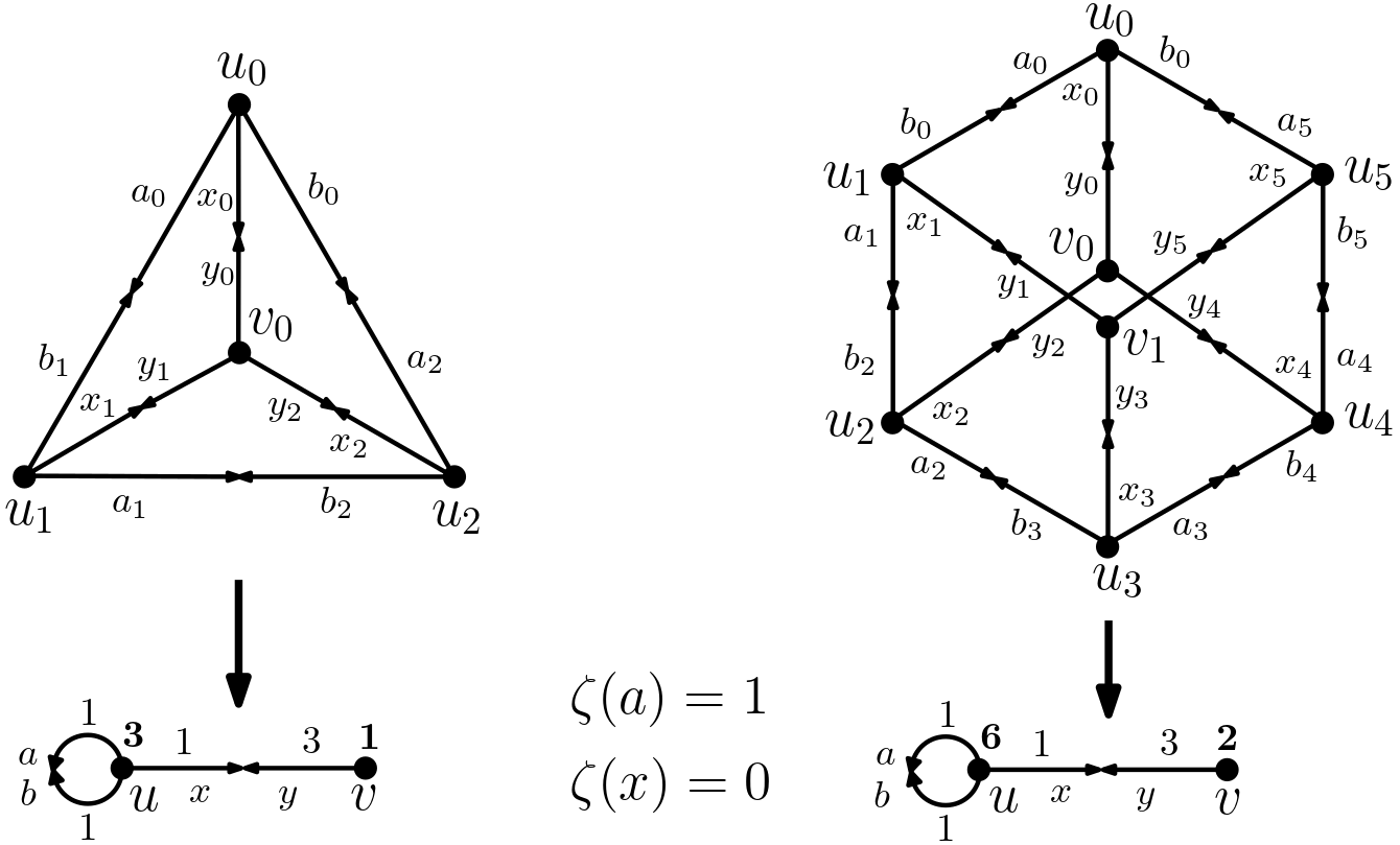
This construction is illustrated in Figure 3.1. Consider the cyclic generalised voltage graph with darts , , and , and vertices and , shown in the bottom left of the figure. Its cyclic generalised cover, , is shown immediately above it. Next to each vertex, in bold lettering, is its image under . This is, and . Then, there are distinct vertices in the fibre of (labelled with ) and a single vertex in the fibre of . Next to each dart is a number indicating its label . Since and , there are darts in the fibre of beginning at each vertex in the fibre of (which consists solely of ). Similarly, for each vertex in the fibre of there is a single dart in each of the fibres of , and , that begins at .
The voltages are given by , and . Consider the dart and see that, by Lemma 3.3 (and since , and ) each vertex is adjacent to all vertices such that modulo . This is, each is adjacent to . By the same token, but considering the dart , we see that each is adjacent to . Finally, Lemma 3.3 also tells us that is adjacent to all , and .
3.2. Extendability of labelled graphs
We now turn our attention to the question of which labelled graphs are extendable (in the sense of Definition 3.1) and which functions then satisfy condition (3.1). This will then allow us to describe a cyclic generalised voltage graph in a more economical manner.
For a function and a walk of , let
| (3.5) |
Then clearly
| (3.6) |
for every two walks for which the concatenation is defined.
Now observe that if is a function which together with satisfies the condition (3.1), then a repeated application of (3.1) to the darts of the walk implies that
| (3.7) |
In particular, for every closed walk . This observations has the following useful consequence.
Lemma 3.5.
A labelled graph is extendable if and only if for every closed walk of .
Let , and suppose that is extendable. Then a function satisfying (3.1) and such that exists if and only if is divisible by , where is the smallest integer for which for one (and thus every) -walk . Such a function is then unique.
Proof.
Fix a vertex of . Suppose first that is extendable and that is a function that together with satisfies (3.1). In view of (3.7), it follows that for every closed walk . Moreover, if , then where is an arbitrary -walk. Since is an integer, this implies that is divisible by . Since this is true for every vertex , we see that is divisible by , as claimed.
Suppose now that for every closed walk . Let and suppose that and are two -walks. Then is a closed walk and hence . But then, in view of (3.6), .
Now choose a -walk , let be the smallest integer such that and let
| (3.8) | |||||
| (3.9) |
In view of the the above argument, we see that this defines and independently of the choice of the -walk .
Remark 3.6.
Note that the condition in Lemma 3.5 only needs to be checked for all cycles . To see that, assume that for every cycle of and let be a closed walk of shortest length such that . Then is not a cycle. However, is a reduced walk since otherwise, by removing a pair of consecutive mutually inverse darts, we obtain a shorter walk with , a contradiction. Hence there are , with . Let and . By the minimality of , we see that for all . On the other hand, clearly , a contradiction.
Moreover, an easy argument (which we leave out) shows that is suffices to check the condition on any complete set of fundamental cycles (recall that a complete set of fundamental cycles relative to a fixed spanning tree is the set of all cycles that contain exactly one cotree dart).
Remark 3.7.
The function that we define in the proof of Lemma 3.5 is such that is the least positive integer such that is an integer for all . It follows that . This has two straightforward but important consequences. First, if is any function that together with satisfies (3.1), then for some positive integer . Second, from Theorem 6.8, we see that , where is defined to be on every dart, is a connected graph.
3.3. Depicting cyclic generalised voltage graphs
We will try to be as economical as possible when drawing a cyclic generalised voltage graph . We will draw every edge simply as a line segment connecting its endpoints, every loop as a closed curve beginning and ending at its unique endpoint, and every semi-edge as a pendant line segment. We will write the label near to each dart that belongs to an edge, so an edge will have two labels, one next to each of its endpoints. We will omit the label on a dart whenever . Moreover, since the index function is completely determined by its image on one vertex, it suffices to specify the image of on a distinguished vertex . We will often use the letter to denote . To indicate voltages, we will draw an arrowhead in the middle of every loop or edge . We will write next to the arrowhead if it is oriented from to (otherwise, we will write ). We will omit the voltage on edges and loops having trivial voltage. A semi-edge with no specified voltage in the picture will be assumed to have voltage .
We now provide an example that illustrates the above described economical way of depicting the cyclic generalised voltage graphs and describe the cyclic generalised cover arising from it in as much an intuitive way as possible.
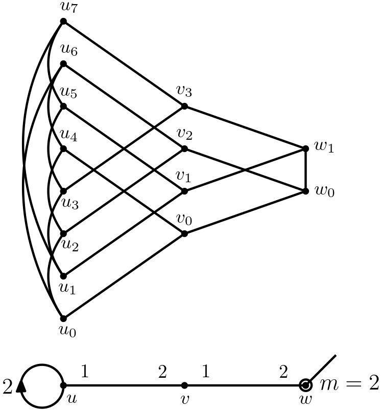
Consider the cyclic generalised voltage graph in the bottom of Figure 3.2, consisting of three vertices , and , and having one loop attached to the vertex , two ordinary edges linking with and with , respectively, and a semi-edge attached to . We will explain how it gives rise to its cyclic generalised cover.
The index function is given as follows. First, note that is the distinguished vertex and has a positive integer (in this case ) assigned to it. This indicates that or, simply put, that the vertex gives rise to distinct vertices in (the fibre above ). The images of other vertices under (and thus also the size of the fibres above those vertices) are determined by . Recall that for all darts we have . By letting be the dart beginning at and ending at we have , and so . Similarly, .
Adjacency rules are given by Lemma 3.3. Recall that an edge lacking an arrowhead indicates that both darts comprising it have trivial voltage. For instance all darts in the edge between and , as well as those in the edge between and , have trivial voltage. We see that a vertex is adjacent to all vertices such that . This is each is adjacent to and . Similarly each is adjacent to and . Now, the loop at has an arrowhead with the number written next to it. This is, one dart in the loop at has voltage while the other has voltage (or equivalently, , since the indices of the vertices in are taken modulo ). Then every is adjacent to and . Finally, the semi-edge at has no specified voltage in the picture. This means that it has voltage . Then every vertex is adjacent to .
4. Classification theorem
We now use the language of cyclic generalised covers to present a classification of all connected simple cubic graphs admitting an automorphism with at most three vertex-orbits.
Definition 4.1.
Let be a cyclic generalised voltage graph. We say that is a cyclic cubic voltage graph (or simply a -graph) if is a simple connected cubic (that is, -regular) graph.
Let us now turn our attention to Figure 4.1. The graphs depicted here, which we denote by for , are all the dart-labelled graphs on at most vertices that can be extended to a ccv-graph. The proof that this family of dart-labelled graphs is indeed complete is postponed until Section 7, where it was obtained by checking all the graphs on at most vertices and maximal valence at most , and then for each of these graphs finding all the labelings satisfying the conditions given in Proposition 7.1 (note that this is a finite problem for each graph). For each dart-labelled graph we have chosen a distinguished vertex shown as a white vertex with a black circle around it and the letter next to it. A voltage assignment, which may assign values or to some darts, has also been specified in the drawing.

Let and let . We define (alternatively or ) as the cyclic generalised cover of the cyclic generalised voltage graph where , is the index function defined by , where is the distinguished vertex of , and is the voltage assignment shown in the picture, where we take the voltage of a semi-edge to be . We will also assume that the integers , and satisfy the conditions listed underneath in Figure 4.1. As we will see in Section 7, these conditions are sufficent and necessary for to be a -graph. Hence, the graph (or or , accordingly) is a connected, cubic, simple graph. We will say that a graph is a ccv-cover of for some if is isomorphic to (or or , accordingly).
Consider for instance the labelled graph . The covering graph is the cyclic generalised cover of the ccv-graph obtained by assigning voltage to (one dart underlying) the loop and letting . Then, if is the remaining vertex, we see that . Observe that the ccv-graph thus obtained is precisely the generalised cyclic voltage graph shown in the bottom left of Figure 3.1. Then is isomorphic to , as shown in the figure. Similarly, is isomorphic to the cube (see Figure 3.1). The graph constructed in the example in the end of the preceding chapter and shown in Figure 3.2 is the graph .
The proof of the following theorem will be given in Section 7.2.
Theorem 4.2.
A graph is a connected, cubic, simple graph with a cyclic group of automorphisms having at most orbits on vertices if and only if it is isomorphic to one of the following:
- (1)
, , , , or ;
- (2)
with even, , , ;
- (3)
with , even, , ;
- (4)
with , , ;
- (5)
with ;
- (6)
with , , , ;
- (7)
with , , ;
- (8)
with even, , ;
- (9)
with even, , ;
- (10)
with even, ;
- (11)
with , even, , , .
5. Generalised covers
In this and next section we prove that cyclic generalised voltage graphs are a special case of a much more general notion of a generalised voltage graph. This fact will come useful in Section 6, where we translate several facts about generalised voltage graphs proved in [22] into the language of cyclic generalised voltage graphs.
For a group , we let denote the set of all subgroups of and for , we let be the conjugate of by . The core of a subgroup in a group , denoted is the intersection of all the conjugates of . We can now present the notions of the generalised voltage graph and of the generalised cover introduced in [22].
Definition 5.1.
Let be a connected graph, let be a group, and let and be two functions such that the following hold for all :
| (5.1) | |||
| (5.2) | |||
| (5.3) |
We then say that the quadruple is a generalised voltage graph and we call the functions and a weight function and a voltage assignment, respectively. The generalised voltage graph is faithful provided that
Definition 5.2.
Let be a generalised voltage graph and let be the graph defined by:
- •
;
- •
;
- •
;
- •
.
Then is called the generalised cover arising from and is denoted by .
The following theorem is the crucial fact of the theory of generalised covers and states that a graph admitting a group of automorphisms can be reconstructed from a voltage graph (for some appropriate and ). This theorem follows directly from Theorem 14 and Remark 17 of [22].
Theorem 5.3.
Let be a graph and let . Then there exist functions and , such that is a faithful generalised faithful voltage graph and is isomorphic to the associated generalised covering graph .
6. Cyclic generalised covers as a special case
Let be a faithful generalised voltage graph. Since is cyclic, every subgroup , is determined uniquely by its index in . This allows us to define two functions and such that is a cyclic generalised voltage graph and . Informally, we can think of a cyclic generalised voltage graph simply as a particular type of a generalised voltage graph. Let us make this more precise.
Let be the cyclic group of integers modulo , and let be a generalised voltage graph. Define and by
| (6.1) | ||||
| (6.2) |
Now observe that is the subgroup generated by , where we view the integer as an element of . Similarly, is generated by its index in , which equals . Hence, the function can be reconstructed from the integer valued functions and using the formulas
| (6.3) | ||||
| (6.4) |
Furthermore, if the generalised voltage graph is faithful, the order of is determined by the functions and , as shown in the lemma below.
Lemma 6.1.
If is a generalised voltage graph, then it is faithful if and only if
| (6.5) |
Proof.
Let . By definition, is faithful if and only if . Since is abelian and since , this is equivalent to the condition that the group
is trivial. Observe that is precisely the subgroup of generated by . Finally, if and only if . ∎
The discussion so far allows us to define a function which assigns to each faithful generalised voltage graph a cyclic generalised voltage graph where and are given by (6.1) and (6.2). Conversely, one can define a mapping that assigns to each cyclic generalised voltage graph, a faithful generalised voltage graph , where and are given by (6.3), (6.4) and (6.5). The mappings and are inverse to each other.
Theorem 6.2.
Let be a generalised voltage graph and let . Then .
Proof.
Let be given by
where the coset of is written in additive notation and the subindex of is taken modulo . To see that is well defined suppose . Then which implies that . This is . It is straightforward to verify that is indeed an isomorphism. ∎
We devote the remainder of this section to stating some fundamental properties of cyclic generalised covers. Each proposition hereafter is a special case, where the voltage group is cyclic, of a more general proposition for a generalised voltage graph proved in [22]. We state these results here in the language of cyclic generalised voltage graphs. Even though each of the following propositions is simply a translation of a (special case of a) proposition stated and proved in [22], we provide a sketch of a proof for Theorems 6.8 and 6.9, as in these cases the translation might not be straightforward.
Lemma 6.3.
[22, Lemma 18] Let be a cyclic generalised voltage graph, let and let . For an element the mapping given by is an automorphism of whose orbits (on vertices and darts) are precisely the fibres of . Moreover, the group homomorphism mapping every to is an embedding.
Lemma 6.4.
[22, Lemma 21] Let be a cyclic generalised voltage graph and let . For an integer coprime to let be given by the rule . Then .
Lemma 6.5.
[22, Lemma 22] Let be a cyclic generalised voltage graph, let , let and let be an integer coprime to . If for every and , for every . Then the permutation mapping a dart to the dart for every extends to an automorphism of .
Theorem 6.6.
[22, Theorem 26] Let be a cyclic voltage graph and let be a spanning tree of . Then there exists a voltage assignment such that for all and .
Definition 6.7.
A voltage assignment in which for all darts belonging to a prescribed spanning tree (as is in the lemma above) is said to be -normalised.
Theorem 6.8.
[22, Theorem 32] Let be a cyclic generalised voltage graph where is -normalised for some spanning tree of . Let and . Then, is connected if and only if .
Proof.
Let and let . Then is connected if and only if is connected. By Theorem 32 of [22], is connected if and only if where and . However, is precisely the subgroup of generated by . Hence is connected if and only if . This equality, in turn, holds if and only if . Since is a multiple of for all , we see that . This completes the proof. ∎
Theorem 6.9.
[22, Theorem 37] Let be a cyclic generalised voltage graph and let . Then is a simple graph if and only if for all darts all of the following conditions hold:
- (1)
for all .
- (2)
for any two parallel darts .
- (3)
for all darts in a semi-edge.
Proof.
Let and let . Then is simple if and only if is simple. Let . Set , and . Note that , and are the smallest integers such that , and . By Theorem 37 of [22] (and by the fact that is abelian), is simple if and only if the three following conditions hold:
- (1’)
for all ;
- (2’)
for all darts , , which are parallel to in and for all ;
- (3’)
if .
We will show that items (1), (2) and (3) of Theorem 6.9 are respectively equivalent to items (1’), (2’) and (3’) above.
Suppose (1’) holds. Then, since is abelian, for all we have . From (5.1) (and again from the fact that is abelian), and so . This is . Now, and by equation (3.1). Hence if and only if . The latter equality holds if and only if . Therefore (1) holds if and only if (1’).
Now, let be parallel to . Suppose (2’) holds. Then, for all , . In particular, and so cannot divide . It follows that modulo . Finally, recall that . Thus (2) holds. Conversely, suppose . If for some for some we have , then, since divides both and , must also divide , a contradiction. Thus (2’) holds. We conclude that (2) is equivalent to (2’).
Finally, it is a plain observation that (3) is equivalent to (3’). ∎
7. ccv-graphs and the proof of Theorem 4.2
7.1. ccv-graphs
Recall that a ccv-graph is a cyclic generalised voltage graph such that its covering graph is simple, connected and cubic; see Definition 4.1. In view of Theorem 6.6, we will assume that is -normalised for some spanning tree . Furthermore, in light of the results in the preceding section, a cyclic generalised voltage graph is a -graph if and only if and agree with Theorems 6.8 and 6.9, and if for all we have
| (7.1) |
see formula 3.3. Let be a dart-labelled graph and recall that can be extended to a cyclic generalised voltage graph if there are functions and satisfying (3.1) and (3.2), respectively. It is a plain observation that the cyclic generalised voltage graph thus obtained might not be a ccv-graph (this is, the covering graph need not be simple, connected or cubic). Then, in order to prove Theorem 4.2, we must determine sufficient and necessary conditions on the dart-labelling for to be extendable to a ccv-graph.
Proposition 7.1.
Let be a connected dart-labelled graph and suppose it is extendable. Then can be extended to a ccv-graph if and only if the following holds:
- (1)
for all vertices .
- (2)
implies .
- (3)
for any two parallel darts and .
- (4)
for every dart underlying a semi-edge.
Proof.
Suppose there are functions and such that is a ccv-graph. Observe that (1) holds by formula (7.1). Now suppose for some . By item (1) of Theorem 6.9, we have . Hence, (2) holds. Now suppose are two parallel darts. By (1), , so either or and . In the latter case, from (3.1) we have . Then is even and . This is , contradicting item (2). Then (3) holds. Finally, item (4) follows at once from item (1) of Proposition 6.9.
For the converse suppose satisfies conditions (1)–(4). Suppose is a dipole with vertices and . Let , and let be the set of darts incident to . By letting and for all , we obtain a ccv-graph .
Now, suppose is not a dipole. Let be the index function given by (3.8) and (3.9) in the proof of Lemma 3.5. Let be the smallest positive integer such that is even if is incident to a semi-edge or to a pair of parallel links, and if is incident to a loop. Define by for all .
To define an appropriate voltage assignment, let and let be a maximal simple subgraph of (note that always exists and can be found by removing all darts, all loops and one edge from each pair of parallel edges in ). Let be a subset of containing exactly one dart for each edge of . Define as follows:
We can now extend to a voltage assignment by letting if and if . It is straightforward to see that satisfies (3.2) and that it is -normalised. Therefore, is a cyclic generalised voltage graph. We leave to the reader to verify that is indeed a ccv-graph. ∎
Let be a -graph and let be an edge of . Then we say is an edge of type , or simply a -edge (note that the order in which we write is important). If and then we will also say, when there is no possibility of ambiguity, that is a -edge. The following is a direct consequence of Proposition 7.1,
Corollary 7.2.
A -graph only has edges of type , , and . In particular, parallel edges in a ccv-graph are necessarily -edges.
Recall that we will always assume a voltage assignment to be trivial on a prescribed spanning tree of ; see Theorem 6.6. In the particular case of ccv-graphs we can chose this tree so that it contains all -edges with . Even further assumptions, stated in Lemma 7.4 at the end of this subsection, can be made about , so that is ”as nice as possible”.
We say a dart-labelled graph is a subgraph of if and is the restriction of to .
Proposition 7.3.
Let be a -graph. Then has a spanning tree that contains all the -edges with .
Proof.
Let be the subgraph of induced by all -edges of with . We will show that is acyclic. Suppose to the contrary that contains a cycle . Let be the the vertex of with the least index, that is for all . Let and be the two neighbours of in . Now, cannot be a -edge as contains no such edges. If is a -edge with , then , which contradicts having minimal index. Hence, must be a -edge with . Similarly, is a -edge with . This implies that the sum of the labels of darts in is at least , contradicting formula (7.1). Hence, is acyclic and thus can always be completed to a spanning tree of . ∎
Lemma 7.4.
Let be a ccv-graph. Then there exists a voltage assignment such that and for all , the following holds:
- (1)
for all ;
- (2)
is -normalised for a spanning tree of containing all -edges with ;
- (3)
whenever underlies a semi-edge;
- (4)
and whenever underlies a loop.
Proof.
By Proposition 7.3, admits a spanning tree that contains all -edges with . By Theorem 6.6 we can assume without loss of generality that is -normalised. Let be the voltage obtained by reducing modulo for all . By Remark 3.4, . Items (1) and (2) follow at once from our choice of .
Suppose a dart underlies a semi-edge. Then by Theorem 6.9. Moreover since . Then by equality (3.2) we have (), or equivalently, (). Since , we see that is even and . Hence (3) holds.
Finally, if underlies a loop, by Theorem 6.9, () and therefore . Hence (4) holds. This completes the proof. ∎
We call a voltage assignment like in Lemma 7.4 a simplified voltage assignment. Since every simple, connected, cubic graph is the cyclic generalised cover of a ccv-graph with a simplified voltage assignment, we will henceforth always assume that the voltage of a ccv-graph is simplified.
7.2. Proof of Theorem 4.2
We would like to begin by making a few observations about the graphs appearing in Figure 4.1. These graphs comprise the complete list of graphs on at most vertices with a dart-labelling that agrees with Proposition 7.1. Although it is a simple enough computation to be done by hand, in order to avoid human error, we used a computer programme written in SAGE [24] to construct, by brute force, all such graphs (up to label-preserving isomorphism). Then, any ccv-graph on at most vertices can be obtained by extending some to a cyclic generalised voltage graph. In light of Lemma 7.4, when extending a labelled graph to a ccv-graph, we will only consider those voltage assignments that agree with the corresponding voltage shown in Figure 4.1 (that is, a voltage assignment that is trivial on every edge lacking an arrowhead, and that assigns voltage to every semi-edge ). The conditions under each are derived from equalities (3.1) and (3.2), and from Theorems 6.8 and 6.9. Hence, an extension of , for some , is a ccv-graph if and only if and satisfy the corresponding conditions listed in Theorem 4.2 (and agree with the corresponding voltage assignment shown in Figure 4.1).
Let be a connected, cubic, simple graph and suppose it admits a cyclic group of automorphism having at most vertex-orbits. By Theorem 5.3, is the generalised cover of a generalised voltage graph , where the quotient has at most vertices. Since is a cyclic group, by Theorem 6.2, where . Moreover, since is connected, cubic and simple is a ccv-graph. Then is an extension of , for some . That is is isomorphic to (or or ) for some , and satisfying the corresponding conditions listed in Theorem 4.2.
For the converse, let be a ccv-graph obtained by extending one dart-labelled graph from Figure 4.1. Recall that the generalised cover of a ccv-graph is a simple, cubic, connected graph. Moreover, the group , where , acts as a group of automorphism of , and the orbits on vertices and darts under this action are precisely the fibres of (see Lemma 6.3). This completes the proof of Theorem 4.2.
8. Cubic vertex-transitive graphs with a cyclic group having at most orbits
We devote this section to the proof of Theorem 1.1 stated in Section 1. That is, we will show that a connected cubic vertex-transitive graph admitting a cyclic group of automorphisms having at most vertex-orbits is either isomorphic to the Tutte-Coxeter graph or it belongs to one the following infinite families:
- (1)
with , , , ;
- (2)
with , , or and ;
- (3)
with , , ;
- (4)
with and odd;
- (5)
with and , or and , or and .
Let be the set containing the following exceptional graphs: , , the cube , the Petersen graph, the Heawood graph, the generalised Petersen graph , the Pappus graph, the dodecahedron and the generalised Petersen graph (see [15] for definitions and properties of the Pappus graph, the Heawood graph and the generalised Petersen graphs).
We will partition the set into three sets: , and . The reason for this is that a ccv-cover of with is necessarily a -multicirculant for some . We can then resort to the classification of cubic vertex-transitive bicirculants (-multicirculants) [20] and tricirculants (-multicirculant) [21] to deal with ccv-covers of when . For the remaining indices in , we distinguish those for which admits no vertex-transitive ccv-cover (these conform the set ) and those who admit at least one vertex-transitive ccv-cover (these conform the set ). As it transpires, all vertex-transitive ccv-covers of with belong to the set of exceptional graphs. Theorem 1.1 will then follow from Claims 8.1 and 8.2 (which will be proved at the end of this section), as well as the classification of cubic vertex-transitive bicirculants and tricirculants.
Claim 8.1.
If , then a vertex-transitive ccv-cover of must be one of the exceptional graphs in .
Claim 8.2.
If then admits no vertex-transitive ccv-cover.
We will now introduce the concept of the signature of a cubic graph, which we will need to prove the claims above. Let be a simple cubic graph. For an edge of and a positive integer denote by the number of -cycles (cycles of length ) that pass through . For a vertex of , let be the set of edges incident to ordered in such a way that . The triplet is then called the -signature of . If for a positive integer all vertices of have the same -signature, we say that is -cycle-regular. In particular, if is -cycle-regular, where is the girth of , we will say that is girth-regular, following the nomenclature of [23]. Observe that if is vertex-transitive, then is -cycle-regular for all .
We will need the five following lemmas. Lemma 8.3 is proved in [23]. Lemma 8.4 is almost folklore, it is mentioned in [8] and [15] but a direct proof is not provided. It follows as a corollary of Theorem 5 of [23]. Meanwhile, Lemma 8.5 is proved in [15]. We provide full proof of Lemmas 8.8 and 8.9.
Lemma 8.3.
[23, Theorem 5] Let be a cubic girth-regular graph of girth . Then either the -signature of is or one of the following occurs:
- (1)
and ;
- (2)
and is isomorphic to a prism or a Möbius ladder;
- (3)
and is isomorphic to the Petersen graph or the Dodecahedron.
Lemma 8.4.
If is a cubic arc-transitive graph of girth smaller than , then is isomorphic to one of the following: , , the three-dimensional cube , the Petersen Graph or the Dodecahedron.
Lemma 8.5.
[15, Proposition 4.2] If is a cubic arc-transitive graph of girth then every edge of lies in exactly cycles of length , or is isomorphic to one of the following graphs: the Heawood graph, the Pappus graph or the generalised Petersen graph with .
Before we state and prove Lemma 8.8, we need to look briefly into the set of exceptional graphs and the possible dart-labelled graphs from which they arise. This will also be used in the proofs of Claims 8.1 and 8.2. For each graph in , we have determined, with the aid of a computer programme written in SAGE [24], the values of for which is a cyclic generalised cover of . For instance, is a cyclic generalised cover of and (and of no other ). Indeed, is isomorphic to and to . The results are displayed in Table 1 below.
| Graph | Cover of | Graph | Cover of |
|---|---|---|---|
| Pappus | |||
| Petersen | |||
| Heawood |
Remark 8.6.
Each graph in is a ccv-cover of for some , and thus is a -multicirculant for some .
Remark 8.7.
Let be a ccv-graph with an edge of type or . If is vertex-transitive, then it is arc-transitive. Indeed, suppose for some , and let . Then all three darts in beginning at a fixed vertex belong to the same orbit under the action of (recall that contains a copy of , with , that acts transitively on the fibres of ). Since is vertex-transitive, this must be true for all vertices. This is, all the three darts beginning at any vertex belong to the same -orbit. Thus is edge-transitive. Finally, it is well known that graph with odd valency that is both vertex- and edge-transitive must also be arc-transitive.
Lemma 8.8.
Let be a -graph. Let be adjacent through a -edge, and suppose is incident to a loop. If is vertex-transitive then it isomorphic to the Heawood graph or the Pappus graph.
Proof.
First, suppose is a -edge consisting of two darts: beginning at , and beginning at . Let be a loop incident at . Let be the number of -orbits on darts. Since , then for every vertex there are precisely two darts in incident to . These two darts must belong to the same -orbit, since has a cyclic subgroup of automorphism acting transitively in each fibre. Since is vertex transitive, the orbits of on darts are precisely the orbits of , the stabiliser of in , on its action on the darts beginning at . Then, has at most orbits on darts. Suppose . Then has two orbits on darts, say and , and since is vertex-transitive, every vertex of is incident to precisely one dart in and two darts in . Hence . Moreover, for every dart both and its inverse belong to the same -orbit (for otherwise every edge of has one dart in and the other in , which implies that , a contradiction). In particular, this implies that both and are subsets of . On the other hand, as , and so . Then, all three darts incident to a vertex lie in the same -orbit, contradicting that . Therefore and is arc-transitive.
Let (that is, ) and recall that is the dart beginning at and ending at . Since there must be another dart, say , incident to . Since is a -edge, we see that . Recall that , as is a -edge (see Lemma 7.4), and let . Notice that for all and all
| (8.1) |
is a -cycle in (see Figure 8.1, left). In particular lies in distinct -cycles, namely and . Furthermore, also lies on both and . Since is arc-transitive, must lie in a -cycle . It is plain to see that must visit either or . This is, one of the edges incident to lies in at least distinct -cycles and by Lemma 8.5, is isomorphic to the Heawood graph, the Pappus graph or the generalised Petersen graph with . However the generalised Petersen graphs with are ccv-covers of only when (see Table 1) and has no edges of type . Therefore must be isomorphic to the Pappus graph or the Heawood graph.


Let and be two graphs and let and be two dart labellings for and respectively. We say the dart labelled graphs and are isomorphic if is there is a graph isomorphism such that .
For , let be the corresponding dart-labelled graphs shown in the bottom row of Figure 8.2, so is a a edge with a loop attached to one of its endpoints and so on. Recall that if is a ccv-graph and , then the covering projection maps every to , for . In addition, recall that if and are dart-labelled graphs, then say is a labelled-subgraph of (and we write ) if is a subgraph of and .
Lemma 8.9.
Let be a ccv-graph and let . Let and suppose for some .
- (1)
If , then is a union of -cycles.
- (2)
If , then is a union of -cycles.
- (3)
If then is a union of copies of .
Proof.
Suppose . If then contains a -edge, say , where is incident to a semi-edge. Recall that all -edges with have trivial voltage in a ccv-graph. Then by Lemma 3.3, every is adjacent to and where . Moreover, every is adjacent to . Hence for all , is a -cycle (see Figure 8.2). It is plain to see that is the union of all such -cycles. The cases when equals , and follow from an analogous argument. ∎
Proof of Claim 8.1. Let and suppose is a vertex-transitive ccv-cover of . If then by Lemma 8.8 we have . If then by Lemma 8.9 the girth of is at most and by Remark 8.7 is arc-transitive. Then, by Lemma 8.4, . If , then by Lemma 8.9 has -signature , where , and by Lemma 8.3 is isomorphic to , which is in . It remains to see what happens when . Suppose is a vertex-transitive ccv-cover of . Then, by Theorem 4.2, is isomorphic to for two integer such that is even and . With the notation of Figure 8.3 (right), let and let be the girth of . Observe that the vertex lies on two distinct -cycles, namely and . This is, every edge incident to lies on a -cycle. If then by Lemma 8.3, is isomorphic to the Petersen graph or the dodecahedron, and we are done since both graphs are in . Clearly, as no vertex in lies on a -cycle (vertices in are only adjacent to vertices in , which is an independent set). If then must lie on a -cycle. It is not too difficult to see that this can only happen if and . However, is then a -cycle, contradicting . We conclude that if , then . We have shown that if , then a vertex-transitive ccv-cover of must be an exceptional graph belonging to .

Proof of Claim 8.2. Let and suppose is a vertex-transitive ccv-cover of . Since no element of is a ccv-cover of for (see Table 1) we see that . Suppose . Then by Lemma 8.9, the girth of is or and by Remark 8.7, is arc-transitive. It then follows from Lemma 8.4 that , a contradiction. If then by Lemma 8.9, has -signature , with , and by Lemma 8.3 we see that is isomorphic to , which is a element of , leading us again to a contradiction. If then by Lemma 8.9, Remark 8.7 and Lemma 8.4 we see, once more, that . If , by Lemma 8.8. The cases when require slightly deeper analysis. In the subsequent paragraphs, we will assume the vertices of the graphs , with , are named as follows: in Figure 4.1, let be the leftmost vertex; the top vertex; the bottom vertex, so that is in fact the distinguished vertex of .
Suppose . Then for some integers such that is even and . Let . By Lemma 8.9 every vertex in lies on a -cycle. Then must also lie on a -cycle . Note that since a vertex is the only neighbour of in , all three vertices in must belong to . This is, or . Then (). However, by item (1) of Lemma 7.4, which implies that either or . Moreover, since , then necessarily and . The reader can verify that the graph is not vertex-transitive.
Now, suppose . Then for some integers such that is even and . Let and let be the girth of . Note that must be arc-transitive as has a -edge. If then by Lemma 8.4, , a contradiction. Suppose . Let be the subgraph induced by . It is plain to see that contains a -cycle (see Figure 8.3, left) and thus . Moreover, every edge incident to , , lies on two distinct -cycles of . The edge also lies on two distinct -cycles, both contained in . Since is arc-transitive, the edge must lie on a -cycle . However, must necessarily visit either or . This is, one of or lies on three distinct -cycles. It follows that the -signature of is not and by Lemma 8.5, , a contradiction.
Finally, suppose and is isomorphic to where is even, and . Let and let be the girth of . Observe that must be arc-transitive since has a -edge. If , then by Lemma 8.5, , a contradiction. Suppose and see that if () then is a -cycle, contradicting our assumption that . Hence we may assume (). Now, note that . Then the voltage of the semi-edge at must be . This implies that each is adjacent to , and in particular that is a -cycle of . Then must also lie on a -cycle . Since both and are independent sets, if a cycle visits twice, it must have length at least . It follows that is the only vertex in belonging to . It is straightforward to see that a -cycle through must necessarily be , for some . This is, in Figure 8.3 (middle), the dotted lines must be edges. This implies that (). Moreover, since we see that . Then the edge lies on both and , which are distinct cycles since (). Since also lies in , it follows from Lemma 8.5 that , once more a contradiction. This completes the proof of Claim 8.2.
Proof of Theorem 1.1. Let be a simple, connected, cubic graph admitting a cyclic group of automorphism with at most orbits on vertices. Suppose is vertex-transitive. Then, is a ccv-cover of for some . By Claim 8.2, . If , then by Claim 8.1, must be one of the exceptional graphs in . However, every graph in is either isomorphic to the Tutte-Coxeter graph or belongs to one of the five infinite families described in Theorem 1.1. Indeed, , , , , the Heawood graph is isomorphic to , , the Pappus graph is isomorphic to and . It remains to see what happens when .
If , then for some integers and where , is even, and (see Theorem 4.2). Observe that . If then is a unit in the ring . That is, has a multiplicative inverse in , and . Then by Lemma 6.5, . On the other hand, if , then is a unit in and, once again by Lemma 6.5, .
Suppose . Note that for integers , and , the graphs and correspond, respectively, to the graphs and described in [20]. It then follows from Proposition 4 of [20] and Theorem 4.2, that if then , for some and (), or and . By the same token, if then where , and . If then by [20, Section 3], is a circulant and so is also a ccv-cover of .
Now, suppose . Observe that the graphs , , and correspond to the graphs , , and described in [21]. By Theorem of [21], if then is isomorphic to with odd. By the same theorem if then with and , or and , or and . If then by Theorem 50 of [21] is also a cover of . Finally if then by Theorem 52 of [21] has order smaller than and by Section 3 of [21], isomorphic to Tutte-Coxeter graph (referred to as Tutte’s 8-cage in [21]).
For the converse, suppose is the Tutte-Coxeter graph or belongs to one of the infinite families described in Theorem 1.1. It is well known that the Tutte-Coxeter graph is arc-transitive and thus also vertex-transitive. A cover of must be vertex-transitive as it has a cyclic group of automorphism with a single orbit on vertices. It is shown in Theorem 4 of [20], that the graphs belonging to the families of items (2) and (3) of Theorem 1.1 are vertex-transitive. Finally, the graphs in items (4) and (5) of Theorem 1.1 are vertex-transitive by Theorem 1 of [21]. This completes the proof.
References
- [1] B. Alspach, T. D. Parsons, A construction for vertex-transitive graphs, Canadian J. Math. 34 (1982), 307–318.
- [2] A. Ádám, Research problem 2–10, J. Combin. Theory, 2 (1967), p. 393.
- [3] A. D. Mednykh, I. A. Mednykh, The number of spanning trees in circulant graphs, its arithmetic properties and asymptotic Discrete Math. 342 (2019), 1772–1781.
- [4] S. Bhoumik, E. Dobson, J. Morris, On the automorphism groups of almost all circulant graphs and digraphs., Ars Math. Contemp. 7 (2014), 487–506.
- [5] P. J. Cameron, M. Giudici, G. A. Jones, W. M. Kantor, M. H. Klin, D. Marušič, L. A. Nowitz, Transitive permutation groups without semiregular subgroups, J. Lond. Math. Soc. 66 (2002) 325–333.
- [6] B. Frelih, K. Kutnar, Classification of cubic symmetric tetracirculants and pentacirculants, Euro- pean J. Combin. 34 (2013) 169–194.
- [7] M. Conder, R. Grande, On embeddings of circulant graphs, Electron. J. Combin. 22 (2015), no. 2, Paper 2.28, 27 pp.
- [8] M. Conder, R. Nedela, Symmetric cubic graphs of small girth, J. Combin. Theory Ser. B 97 (2007), 757–768.
- [9] M. Giudici, I. Kovács, C.-H. Li, G. Verret, Cubic arc-transitive k-multicirculants, J. Combin. Theory Ser. B 125 (2017), 80–94.
- [10] R. Jajcay, Š. Miklavič, P. Šparl, G. Vasiljević, On certain edge-transitive bicirculants, Electron. J. Combin. 26 (2019), no. 2, Paper 2.6, 28 pp.
- [11] I. Kovács, B. Kuzman, A. Malnič, S. Wilson, Characterization of edge-transitive 4-valent bicirculants, J.’ Graph Theory 69 (2012), 441–463.
- [12] D. Marušič, On vertex symmetric digraphs, Discrete Math. 36 (1981) 69–81.
- [13] D. Marušič, Strongly regular bicirculants and tricirculants Ars Combin. 25 (1988), 11–15.
- [14] Y.-L. Qin, B. Xia, S. Zhou, Stability of circulant graphs, J. Combin. Theory Ser. B 136 (2019), 154–169.
- [15] Y.-Q. Feng, R. Nedela, Symmetric cubic graphs of girth at most 7, Acta Univ. M. Belii Ser. Math. 13 (2006), 33–35.
- [16] J. Gross , T. W. Tucker, Topological graph theory, Wiley-Interscience, New York, NY, (1987).
- [17] M. Hladnik, D. Marušič, T. Pisanski, Cyclic Haar graphs, Discrete Math. 244 (2002), 137–152.
- [18] A. Malnič, R. Nedela, M. Škoviera, Lifting graph automorphisms by voltage assignments, Europ. J. Combin. 21 (2000), 927-947.
- [19] A. Malnič, D. Marušič, P. Potočnik, Elementary abelian covers of graphs, J. Alg. Combin., 20 (2004), 71–96.
- [20] T. Pisanski, A classification of cubic bicirculants, Discrete Math. 307 (2007), 567–578.
- [21] P. Potočnik, M. Toledo, Classification of cubic vertex-transitive tricirculants, to appear in Ars Math. Contemp.
- [22] P. Potočnik, M. Toledo, Generalised voltage graphs, arXiv:1910.08421.
- [23] P. Potočnik, J. Vidali, Girth-regular graphs, Ars Math. Contemp. 17 (2019) 249–368.
- [24] W. A. Stein et al., SageMath, the Sage Mathematics Software System (Version 8.3), The Sage Developers, 2018, [https://www.sagemath.org].
- [25] J. Širáň, Coverings of graphs and maps, ortogonality, and eigenvectors, J. Alg. Combin. 14 (2001), 57–72.
- [26] M. Škoviera, A contribution to the theory of voltage graphs, Discrete Math. 61 (1986), 281–292.
- [27] P. Spiga, Semiregular elements in cubic vertex-transitive graphs and the restricted Burnside problem, Math. Proc. Cambridge Phil. Soc. 157 (2014), 45–61.