Noise Temperature of Phased Array Radio Telescope: The Murchison Widefield Array and the Engineering Development Array
Abstract
This paper presents a framework to compute the receiver noise temperature () of two low-frequency radio telescopes, the Murchison Widefield Array (MWA) and the Engineering Development Array (EDA). The MWA was selected because it is the only operational low-frequency Square Kilometre Array (SKA) precursor at the Murchison Radio-astronomy Observatory, while the EDA was selected because it mimics the proposed SKA-Low station size and configuration. It will demonstrated that the use of an existing power wave based framework for noise characterization of multiport amplifiers is sufficiently general to evaluate of phased arrays. The calculation of was done using a combination of measured noise parameters of the low-noise amplifier (LNA) and simulated -parameters of the arrays. The calculated values were compared to measured results obtained via astronomical observation and both results are found to be in agreement. Such verification is lacking in current literature. It was shown that the receiver noise temperatures of both arrays are lower when compared to a single isolated element. This is caused by the increase in mutual coupling within the array which is discussed in depth in this paper.
Index Terms:
Aperture arrays, Mutual coupling, Noise receiver temperature, Radio Telescope, Radio astronomyI Introduction

The computation of receiver noise temperature () and radiation efficiency () of a phased array can be complex in nature due to the presence of mutual coupling. However, there are many frameworks for computing it. For example, the computation of using a voltage framework was demonstrated in [1], while other power based methods are covered in [2] and [3] which involves the calculation of available gain of the phased array. For radiation efficiency calculation, power based frameworks were demonstrated in [4, 5, 6].
The two main motivations for being able to calculate prior to building the telescope are, the cost effectiveness of characterizing the telescope and insight into the noise coupling mechanism. Both of these abilities are useful when designing and characterizing next generation radio telescopes such as the Square Kilometre Array (SKA) [7].
The first contribution of this paper is to calculate the of the Murchison Widefield Array (MWA) [8, 9] and the Engineering Development Array (EDA) [10]. The calculated will be validated against measured results obtained via astronomical observations using similar methods seen in [11, 10, 12]. The measured using astronomical observations also includes the effects of mutual coupling. Such comparison are not found elsewhere in literature, which forms the major contribution of this paper.
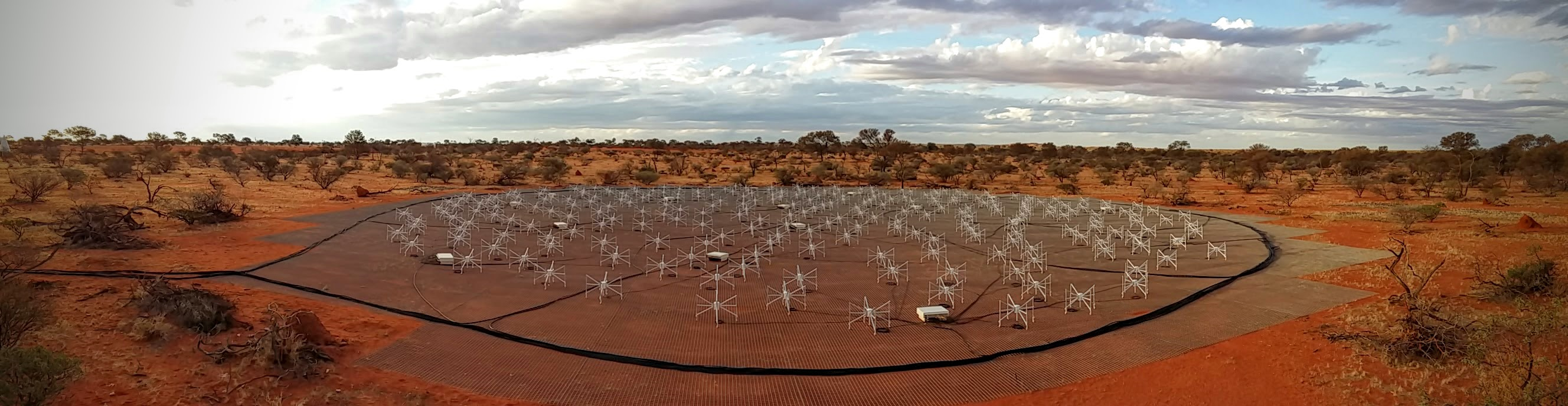
The MWA is the first operational precursor telescope to the SKA-Low located at the Murchison Radio-astronomy Observatory (MRO) in the Shire of Murchison, Western Australia. The telescope consists of 256 phased arrays [9] called ‘tiles’ as shown in Fig 1. Each tile contains 16 antenna elements, called MWA dipoles, placed in a configuration spaced 1.1 apart over a metallic ground mesh. Each element houses a low-noise amplifier (LNA) in the central hub and the output signal travels through a phase matched coaxial cable to the beamformer. The maximum spread of the tiles that make up the overall telescope is approximately 5.3 . The computation of at the tile level is of interest as it is required for determining the sensitivity of the MWA tile [8].
The EDA uses the same dipole elements as the MWA but houses a modified LNA(1)(1) (1) The LNA was slightly modified to have a larger bandwidth (50-300 ). Apart from this slight change, the LNA is identical to that used in the MWA (70-300 ).. The EDA consists of 256 elements placed in a pseudo random configuration spanning 35 diameter over a metallic ground mesh [10] as shown in Fig 2. It was designed to mimic the proposed SKA-Low station configuration and therefore making it a perfect test bed as it shares nearly identical elements to the MWA. The comparison of EDA’s to MWA gives insight of the impact of mutual coupling on which will be presented later.
The can also be measured using the Y-factor method as seen in [13, 14], which uses a sufficiently large absorber as the hot source which covers the main beam and the sky as the cold source. At around the region, the opposite takes place as the average sky temperature is in the thousands of Kelvin. The sky is the hot source while the absorber is the cold source. However, the sky temperature exponentially decays with increasing frequency with a transition frequency at . At the transition frequency, and thus the Y-factor method will fail. In addition, large absorber structure is required to be built which limits the practicality of the Y-factor method to smaller arrays making unsuitable for the MWA tile and the EDA.
The second contribution of this paper is to demonstrate that a power wave based framework (PWF) found in [15] can be recast to compute of a phased array. The fundamental concept of this framework is the computation of incident and reflected power. This method was selected because it is based in the -parameters domain which is more closely connected with the authors previous work in this area [16].
Additionally, the formulation can be easily modified to compute various quantities such as active/embedded reflection coefficient, transducer/available gain, and incident/reflected power of given source(s) that includes all coupling paths. An example of this will be shown by re-using this framework to calculate delivered power to the array for radiation efficiency calculation in subsequent section.
The of an array can be calculated using [4]
| (1) | ||||
| (2) |
where is the available receiver noise power at the output, is the available ambient temperature noise power at the output due to isotropic sky at and is the available gain of the LNA for a single element but for an array, it represents the available receiver gain.
Effectively, both the previously mentioned voltage and power framework works by computing a similar ratio described by (1). The proposed framework for calculating using [15] was shown to be consistent with current methods in [17] when compared to the voltage and power framework found in [1, 3].
The active reflection coefficient () alongside the input referred single element formulation given by (3) can be used as an alternative.
| (3) |
where the four noise parameters are represented by , and .
However, the simple insight given by (3) breaks down when . This over unity condition was achieved by the MWA and EDA at several pointing directions in the region due to the embedded reflection coefficient of the dipoles being close to unity and thus, the active reflection concept will not be discussed further in this paper aside from its links to the proposed framework found in Sect. II-C.
II Receiver and External Noise Calculation
With the aid of Fig. 3, let us consider the sources of noise that exist in the system. Firstly, there is the external noise which consists of noise from the sky due to naturally radiating cosmic sources, soil and thermal noise due to ohmic losses which form a net power flow that is incident onto the Antenna-Receiver Boundary represented by . Secondly, there is the internal noise due to the receiver which produces noise waves indicated by and towards both boundaries [18] and noise waves emerging from the load (not shown in diagram).
For subsequent analysis, it is implied that the properties of the boundary are as follows:
- 1.
it only exists in the absence of a conjugately matched impedance with respect to the left and right hand side of the boundary,
- 2.
the larger the mismatch, the more impenetrable the boundary is to the incident power wave,
- 3.
it is temperature invariant. That is to say, the impedance on either side of the boundary are not affected by changes in physical temperature.
The available internal noise power () in (1) is calculated under the condition that no external noise is present. Conceptually, it implies that the antenna and load is immersed and kept at thermal equilibrium in a 0 isotropic environment. For convenience, internal noise power delivered to a noiseless reference impedance () matched load was computed rather than available power at the output.
Similar treatment is applied for the available external noise power (). The delivered external noise power under the condition that no internal noise is present was calculated. Here, it was assumed that the receiver and load is immersed and kept at 0 while the antennas are kept at thermal equilibrium in an isotropic environment at . Using the relation from (1), it can be shown that
| (4) | ||||
| (5) |
where is the noise power delivered to a noiseless matched load due to internal sources alone, is the noise power delivered to a noiseless matched load due to external sources alone and is the receiver transducer gain. The transducer gain is defined as the ratio of the delivered power by the network to the available power from the source () [19].
This analysis is simple for a single isolated element as the quantity and are easily computed. However, for an array of closely spaced antennas this is no longer the case. In this scenario, the antennas mutually couple and causes to deviate away from a single element case. The mechanisms that cause this overall effect are
- 1.
changing of embedded antenna impedance,
- 2.
coupling of outbound internal noise to neighbouring elements.
Furthermore, the computation of and subsequently for an array is not apparent at first glance due to the complex coupling paths.
II-A Contribution of Internal Noise
Fig. 4 shows an example of noise paths that each noise wave will undergo for a two-element array. All these various paths can be accounted for using matrices to compute the outgoing receiver noise power at the boundaries as follows
| (6) | ||||
| (7) |
where is a noise correlation Hermitian matrix of the outgoing noise power from each port (inputs and outputs) for an -port network, is the noise correlation matrix of the multiport amplifier due to internal sources alone, accounts for the mismatches in impedance, is the Hermitian operator, and are the -parameters of the multiport amplifier and the combined source (antenna) and load network attached to the multiport amplifier respectively. For completeness, the derivation of can be found in Appendix A.
The noise power wave quantities computed by (6) can be visualized with the aid of Fig. 5. Each entry of the matrix contains information of outbound noise power waves (dashed arrows) due to internal sources alone after all coupling paths have been accounted for. The main diagonal contains the total noise power emerging from the network ports due to all and sources, while the cross terms contain the total amount of correlated power between port and .
To compute (6) correctly, , and must have a consistent port numbering convention. Based on the port numbering convention shown in Fig. 5, assuming that
- 1.
- 2.
odd numbered ports are inputs and even numbered ports are outputs of the multiport amplifier network,
- 3.
a reflectionless load () is attached to the outputs of the LNAs then,
For the computation of seen in (4), the delivered noise power to loads at the output of the network are contained in the subset of matrix (6). As the input ports to be odd numbered, all the odd rows and columns to form a submatrix can be removed. This submatrix is the correlation matrix that can be used for characterizing the amount of noise coupling that exists in correlating arrays. To get the total coupled noise power after the summer at the output of a phased array, this submatrix is multiplied by the beamformer weights as follow
| (28) |
where is a row vector containing the applied beamformer complex weights and a submatrix containing even numbered rows and columns of (6). To ensure correct scaling in the calculated output power, the amplitude of is scaled by the number of elements such that .
II-B Contribution of External Noise
The outgoing power wave at the inputs and outputs of the multiport network due to power incident at the input ports are given by
| (29) |
where contains the noise correlation matrix of the attached loads at the input and output of the LNA.
From the perspective of a matched load at the output ports of the multiport network, (29) describes the incident power from the network at the Receiver-Load Boundary. On the other hand, from the perspective of the source at the input ports, (29) describes the reflected power at the Antenna-Receiver Boundary (see Fig. 5).
For passive loads at thermal equilibrium with the noise correlation matrix can be determined by Bosma’s theorem [20] which states that
| (30) |
To simulate noiseless loads being attached at the output of the LNA, in (30) must be replaced by
The assumption of noiseless loads being attached to the output stage does not introduce a measurable change as a well-designed receiver chain should be dominated by LNA noise. The total delivered power from the network to load is given by
| (37) |
II-C Links to Active Reflection Coefficient Concept
Before proceeding further, it is worth discussing links to theory presented in Sect. II-A and II-B to the commonly used active reflection formulation.
The output referred noise temperature calculated using the active reflection coefficient (3) relates to (28) via
| (38) | ||||
| (39) |
where is the number of elements in the array, and are the input referred noise temperature and the transducer gain of the element calculated using (3) and (39) respectively.
The calculated using (41) is exact. This calculation becomes an approximation when attempting to solely use (3) to infer the array noise temperature for cases when and/or is greater than unity. Under this condition the average input referred noise temperature diverges away from the array noise temperature and therefore, it is more general to discuss the behaviour of the array’s output referred noise temperature and the transducer gain separately.
II-D Radiation Efficiency Calculation
Radiation efficiency () of any antenna structure is defined by [4, 5]
| (42) | ||||
| (43) | ||||
| (44) |
where is the total radiated power and is the total injected power into the antenna, is the free space impedance and is the far-field embedded element pattern (EEP) of the antenna as a function of and , is the voltage drop across the antenna, is port current, and represents the element by element multiplication and complex conjugate operator respectively.
As noted in [5], the accuracy of this computation for high efficiency arrays is limited by the numerical sampling and integration of the far-field pattern used to compute . Furthermore, additional data such as port currents and voltage drop across the antenna terminals are required to be saved for the computation of . While the numerical integration is unavoidable, the aim is to reduce the amount of additional data required to be saved and reuse pre-existing data obtained during the characterization of the phased array such as embedded element pattern and -parameter simulation. This provides the additional motivation for this section.
A different approach to compute is to use the pattern overlap integral (POI) method found in [4], which eliminates the need to know the injected power by reversing the problem from a transmit to receive antenna. The EEPs required for the POI method are based on open circuit condition of all neighbouring elements whereas, EEPs generated in [21] are based on loaded condition (LNA input impedance) of all elements. To reuse pre-existing EEPs generated in [21], POI formulation requires modification.
Fig. 6 shows an equivalent circuit of a transmit antenna. The total radiated power captured in the far-field pattern is due to the power dissipated by . This means that the far-field EEP does not directly contain the knowledge of any losses. By reversing the problem to receive mode, the noise power delivered to by at a nominal physical temperature can be determined for a given EEP generated in transmit mode. The total noise power delivered to the array terminated with identical LNA impedances given that the antenna sees an homogeneous sky at is given by
| (45) | ||||
| (46) |
where is the noise correlation matrix due to homogeneous sky that is based on the POI formulation, is the wavelength in meters, and relates the incident electromagnetic wave to the voltage seen at the load of the element as a function of and . The derivation of can be found in Appendix B.
The total noise power delivered to by at physical temperature of can be calculated using Bosma’s theorem [20] or Twiss’s theorem [4]. For our purposes, Bosma’s theorem is a more convenient choice as it uses -parameter natively. This is where the versatility of [15] comes into play. The formulation can easily be modified to calculate the total delivered external noise power at the input of the LNAs using
| (47) | ||||
| (48) | ||||
| (49) |
where is the incident noise power to the LNA due to external sources alone, and were previously computed in (29) and (30).
The radiation efficiency is then given by
| (50) |
This is effectively how the POI method works. For verification, it was shown in [22] that the radiation efficiency calculated using (50) and (42) produced identical results within numerical error. The result is reproduced here with additional verification using perfect electric conductor (PEC) materials.
The efficiency of the MWA as seen in Fig. 7 was calculated using (50). For result verification, these values were compared against those obtained using (42). The numerical integration on the radiation pattern was performed at a resolution of for both methods. Additionally, previous raw simulation data was reprocessed to obtain the port currents required for the computation of .
For the PEC case, the efficiency reported was as high as 100.5% which is due to the limitations of the simulation package. As demonstrated in [5], the efficiency obtained using Method-of-Moments (MoM) based solver such as FEKO for PEC materials ranges from 100% to 100.7%. Efficiency calculation was not done for the EDA as the array was simulated using perfect electric conductor (PEC) material over infinite ground and due to lengthy simulation time, it was not repeated with lossy materials.
III Results
III-A Receiver Temperature
The MWA tile and the EDA were simulated using an electromagnetic simulator FEKO to obtain the -parameter of the arrays. The expected and was calculated for the two arrays using (52) and the measured noise and -parameters of the LNA obtained in [16]. The calculated receiver noise temperature was then compared to values obtained via astronomical drift scan method as seen in [11, 10, 12].
Fig. 8 shows the comparison between the calculated and observed receiver noise temperature of the MWA. The observations were performed on the 9th June 2014 by setting all the MWA beamformes to point overhead (at zenith) and allowing astronomical sources to drift through the MWA’s beam. The expected power detected as a function of frequency () by a phased array is given by
| (51) | ||||
| (52) |
where is the overall power gain of the array signal chain which includes the transducer gain, cable losses, secondary amplication stage etc, is the antenna temperature due to sky noise and is the ambient temperature.
The quantity can be obtained by first modelling the predicted power as
| (53) |
and is estimated as
| (54) |
where is the simulated far-field power pattern as a function of and , is the sky brightness temperature obtained from "Haslam Map" [23] at frequency , which has been scaled down from the original to lower frequencies by multiplying by a factor .
Least square optimization is then performed on the predicted with the observed to solve for and respectively. Based on (53) the power received by every tile is expected to be proportional to , assuming that the sky model used in (54) is a good representation of the true sky (accuracy of sky model is of order ). This relation has been identified to hold best for the 12 to 14 hours range of the Local Sidereal Time (LST) (4)(4) (4) LST is an hour angle between vernal equinox and local meridian (see also [10] for a more detailed justification of LST range selection procedure). Once the calculated values had been obtained, this model is fitted to measured data using least squares to solve for and .
The frequency ranges of to and and above show radio frequency interference (RFI) which causes the observed to increase dramatically. The error bars generated are based on the standard deviation of calculated over MWA tiles used during observation.
III-B Transducer Gain
The most interesting result that emerged from this calculation is the reduction of over the single element at lower frequencies. As shown in Fig. 10, the lowering of can be attributed to increasing as the total internal noise power delivered to the load in the array environment is fairly similar to the single isolated element case. To verify that the results presented remain physically valid, was recalculated for a single isolated element given that the antenna was conjugately matched at all frequencies to the LNA’s input impedance. This calculation sets the absolute upper limit which the of the array must not exceed as it would imply the source is delivering more power than the available source power (). This maximum value was compared to the mean and standard deviation of the array’s over all 197 pointing angles in Fig. 11 and showed that the calculated array remains physically valid.
Similar effects have been observed in the EDA results seen in Fig. 9. However, the reduction of when compared to a single element was not as drastic as the transducer gain did not increase as much as the MWA tile. Standard deviations in Fig. 12 clearly show that in general MWA has a higher transducer gain when compared to the EDA, however the of an MWA tile varies over pointing angles more than the EDA.
The mechanism causing the increasing of can be investigated by plotting the delivered power to the array due to external sources alone as shown in Fig. 13 and 14. It can be observed that additional power is delivered to the array due to mutual coupling at 50 to 170 . It can be clearly seen that for the MWA, the reduction in is due to more external noise power (signal of interest) being delivered to the array. In contrast, the EDA has less coupling, hence less additional power is delivered to the array which leads to less reduction in .
The higher levels of power delivered due to mutual coupling (cross terms) makes the array sensitive to complex weightings applied by the beamformer at the output. This result is consistent with the trend observed in Fig. 12 whereby, the MWA experiences larger changes to with changing pointing angles. Such high level of coupling can be explained by the physical layout of the elements. The element spacing within an MWA tile is from centre to centre whereas for the EDA, the average element spacing is .
Based on these results, it can be reasoned that the reduction of is possible by optimizing the element layout (increased coupling) without having to optimize the LNA over the entire frequency band. Meaning, the LNA could be optimized to cover the mid to high frequency band whereas, the array layout could be optimized to take advantage of the effects of mutual coupling to improve the at lower frequencies (50 - 140 ).
Layout optimization only works if the dominant contribution is due to external noise. That is to say, the if the internal noise is not fluctuating much as a function of complex weightings (see Fig. 10), then increasing the amount of external noise through mutual coupling is beneficial for lowering . In the domain where internal noise dominates, increased mutual coupling is not desirable as this will lead to an increase in . The only way to decrease in this case without changing the antenna design is to optimize the LNA. This reasoning comes with a caveat that it only applies to the MWA dipole design. Other antenna designs were not analyzed which could potentially lead to a different conclusion found here.
IV Conclusion
This paper presents a power wave based framework for analyzing the of an aperture array which includes the effects of mutual coupling. Using a combination of measured noise parameters and simulated -parameters of the MWA tile and the EDA to calculate the receiver noise temperature. The calculated obtained using the proposed PWF was compared with measured obtained via astronomical observations and was found to be in good agreement between the two for both the MWA tile and the EDA. It was observed that due to higher mutual coupling in the region, the MWA has a lower receiver noise when compared to the EDA. The decrease in was due to the increase in transducer gain.
The increased at lower frequencies was due to the additional external noise power delivered to the array via coupling. This improvement was seen for both the MWA tile and the EDA but since the MWA tile has higher coupling, the was lower than the EDA. In addition, higher fluctuation in as a function of pointing angles with higher levels of coupling. For this reason, mutual coupling could either be a hindrance or aid when it comes to reducing depending on whether the internal or external noise dominates the overall contribution.
Additionally, it was demonstrated that the PWF is able to make use of embedded element patterns to calculate the efficiency of the array without the need for re-simulation. In conclusion, the PWF presented in [15] is a general method suited to compute receiver noise temperature for multiport devices and extendable to include phased arrays as demonstrated in this paper. This framework can be utilized to optimize and characterize future generation telescopes such as the Square Kilometre Array [7].
Appendix A Derivation of Matrix
The standard -parameter representation of incident and reflected wave are as shown below.
| (55) | ||||
| (56) |
where is a vector containing the outgoing wave from the the input and output ports of multiport amplifier indicated by the red arrows in Fig. 5, is a vector containing the noise waves and , is the vector containing the reflected wave due to the attached load at the input and output ports of the network, and are the -parameters of the network and loads respectively.
The noise wave vector appears in (55) to represent noise wave originating from the network. By substituting (56) into (55) and solving for yields,
| (57) | ||||
| (58) |
The outgoing power due to internal noise alone is simply given by
| (59) | ||||
| (60) |
where .
Appendix B Derivation of
The quantity is defined as follows
| (61) | ||||
| (62) |
where the effective length () is given by [6]
| (63) |
where is the voltage dropped across the input of the LNA, is the incident plane wave, and are the impedance of the load and antenna under transmit condition respectively, is the angular frequency, is the permeability of free space, is the port current under transmit condition and is embedded element radiation pattern.
ACKNOWLEDGEMENT
The author would like to thank Randall Wayth for useful feedback on this manuscript. The author acknowledges the contribution of an Australian Government Research Training Program Scholarship in supporting this research. The International Centre for Radio Astronomy Research (ICRAR) is a Joint Venture of Curtin University and The University of Western Australia, funded by the Western Australian State government. The MWA Phase II upgrade project was supported by Australian Research Council LIEF grant LE160100031 and the Dunlap Institute for Astronomy and Astrophysics at the University of Toronto. This scientific work makes use of the Murchison Radio-astronomy Observatory, operated by CSIRO. We acknowledge the Wajarri Yamatji people as the traditional owners of the Observatory site. Support for the operation of the MWA is provided by the Australian Government (NCRIS), under a contract to Curtin University administered by Astronomy Australia Limited. We acknowledge the Pawsey Supercomputing Centre which is supported by the Western Australian and Australian Governments.
References
- [1] K. F. Warnick, B. Woestenburg, L. Belostotski, and P. Russer, “Minimizing the Noise Penalty Due to Mutual Coupling for a Receiving Array,” IEEE Transactions on Antennas and Propagation, vol. 57, no. 6, pp. 1634–1644, June 2009.
- [2] M. V. Ivashina, R. Maaskant, and B. Woestenburg, “Equivalent System Representation to Model the Beam Sensitivity of Receiving Antenna Arrays,” IEEE Antennas and Wireless Propagation Letters, vol. 7, pp. 733–737, 2008.
- [3] L. Belostotski, B. Veidt, K. F. Warnick, and A. Madanayake, “Low-Noise Amplifier Design Considerations For Use in Antenna Arrays,” IEEE Transactions on Antennas and Propagation, vol. 63, no. 6, pp. 2508–2520, June 2015.
- [4] K. F. Warnick, M. V. Ivashina, R. Maaskant, and B. Woestenburg, “Unified Definitions of Efficiencies and System Noise Temperature for Receiving Antenna Arrays,” IEEE Transactions on Antennas and Propagation, vol. 58, no. 6, pp. 2121–2125, June 2010.
- [5] R. Maaskant, “Analysis of Large Antenna Systems,” Ph.D. dissertation, Department of Electrical Engineering, Technische Universiteit Eindhoven, 2010.
- [6] K. F. Warnick, R. Maaskant, M. V. Ivashina, D. B. Davidson, and B. D. Jeffs, Phased Arrays for Radio Astronomy, Remote Sensing, and Satellite Communications, ser. EuMA High Frequency Technologies Series. Cambridge University Press, 2018.
- [7] P. E. Dewdney, P. J. Hall, R. T. Schilizzi, and T. J. L. W. Lazio, “The Square Kilometre Array,” Proceedings of the IEEE, vol. 97, no. 8, pp. 1482–1496, Aug 2009.
- [8] S. J. Tingay, R. Goeke, J. D. Bowman, D. Emrich, S. M. Ord et al., “The Murchison Widefield Array: The Square Kilometre Array Precursor at Low Radio Frequencies,” PASA, vol. 30, p. e007, Jan. 2013.
- [9] R. B. Wayth, S. J. Tingay, C. M. Trott, D. Emrich, M. Johnston-Hollitt et al., “The Phase II Murchison Widefield Array: Design overview,” PASA, vol. 35, Nov. 2018.
- [10] R. Wayth, M. Sokolowski, T. Booler, B. Crosse, D. Emrich et al., “The Engineering Development Array: A Low Frequency Radio Telescope Utilising SKA Precursor Technology,” PASA, vol. 34, p. e034, Aug. 2017.
- [11] J. D. Bowman, D. G. Barnes, F. H. Briggs, B. E. Corey, M. J. Lynch et al., “Field Deployment of Prototype Antenna Tiles for the Mileura Widefield Array Low Frequency Demonstrator,” AJ, vol. 133, pp. 1505–1518, Apr. 2007.
- [12] A. T. Sutinjo, T. M. Colegate, R. B. Wayth, P. J. Hall, E. de Lera Acedo et al., “Characterization of a Low-Frequency Radio Astronomy Prototype Array in Western Australia,” IEEE Transactions on Antennas and Propagation, vol. 63, no. 12, pp. 5433–5442, Dec 2015.
- [13] A. Chippendale, D. Hayman, and S. Hay, “Measuring Noise Temperatures of Phased-Array Antennas for Astronomy at CSIRO,” Publications of the Astronomical Society of Australia, vol. 31, p. 14, 01 2014.
- [14] A. P. Chippendale, A. J. Brown, R. J. Beresford, G. A. Hampson, R. D. Shaw et al., “Measured aperture-array noise temperature of the Mark II phased array feed for ASKAP,” in 2015 International Symposium on Antennas and Propagation (ISAP), Nov 2015, pp. 1–4.
- [15] J. Randa, “Noise Characterization of Multiport Amplifiers,” IEEE Transactions on Microwave Theory and Techniques, vol. 49, no. 10, pp. 1757–1763, Oct 2001.
- [16] A. T. Sutinjo, D. C. X. Ung, and B. Juswardy, “Cold-Source Noise Measurement of a Differential Input Single-Ended Output Low-Noise Amplifier Connected to a Low-Frequency Radio Astronomy Antenna,” IEEE Transactions on Antennas and Propagation, vol. 66, no. 10, pp. 5511–5520, Oct 2018.
- [17] D. Ung, A. Sutinjo, and D. Davidson, “Evaluating Receiver Noise Temperature of a Radio Telescope in the Presence of Mutual Coupling: Comparison of Current Methodologies,” in 2019 13th European Conference on Antennas and Propagation (EuCAP), March 2019, pp. 1–3.
- [18] S. W. Wedge and D. B. Rutledge, “Wave techniques for noise modeling and measurement,” IEEE Transactions on Microwave Theory and Techniques, vol. 40, no. 11, pp. 2004–2012, Nov 1992.
- [19] G. Gonzalez, Microwave Transistor Amplifiers: Analysis and Design. Prentice Hall, 1997, ch. 2.
- [20] S. W. Wedge and D. B. Rutledge, “Noise Waves and Passive Linear Multiports,” IEEE Microwave and Guided Wave Letters, vol. 1, no. 5, pp. 117–119, May 1991.
- [21] R. Wayth, T. Colegate, M. Sokolowski, A. Sutinjo, and D. Ung, “Advanced, efficient primary beam modeling for the Murchison Widefield Array radio telescope,” in 2016 International Conference on Electromagnetics in Advanced Applications (ICEAA), Sept 2016, pp. 431–434.
- [22] D. Ung, A. Sutinjo, D. Davidson, M. Johnston-Hollitt, and S. Tingay, “Radiation Efficiency Calculation of the Murchison Widefield Array Using a Power Wave Based Framework,” in 2019 IEEE International Symposium on Antennas and Propagation and USNC-URSI Radio Science Meeting, July 2019, pp. 401–402.
- [23] C. G. T. Haslam, C. J. Salter, H. Stoffel, and W. E. Wilson, “A 408 MHz all-sky continuum survey. II - The atlas of contour maps,” Astronomy and Astrophysics Supplement Series, vol. 47, p. 1, Jan. 1982.