SOS: Selective Objective Switch for Rapid Immunofluorescence Whole Slide Image Classification
Abstract
The difficulty of processing gigapixel whole slide images (WSIs) in clinical microscopy has been a long-standing barrier to implementing computer aided diagnostic systems. Since modern computing resources are unable to perform computations at this extremely large scale, current state of the art methods utilize patch-based processing to preserve the resolution of WSIs. However, these methods are often resource intensive and make significant compromises on processing time. In this paper, we demonstrate that conventional patch-based processing is redundant for certain WSI classification tasks where high resolution is only required in a minority of cases. This reflects what is observed in clinical practice; where a pathologist may screen slides using a low power objective and only switch to a high power in cases where they are uncertain about their findings. To eliminate these redundancies, we propose a method for the selective use of high resolution processing based on the confidence of predictions on downscaled WSIs — we call this the Selective Objective Switch (SOS). Our method is validated on a novel dataset of 684 Liver-Kidney-Stomach immunofluorescence WSIs routinely used in the investigation of autoimmune liver disease. By limiting high resolution processing to cases which cannot be classified confidently at low resolution, we maintain the accuracy of patch-level analysis whilst reducing the inference time by a factor of 7.74.
1 Introduction
Patch-level image processing with convolutional neural networks (CNNs) is arguably the most widely used method for gigapixel whole slide image (WSI) analysis popular. Ordinarily, processing such a large image in its totality with CNNs is computationally infeasible without significant downscaling — resulting in the loss of detailed information required for fine-grained analytical tasks. However, by processing WSIs in smaller patches, it is possible to extract the detailed information by preserving the resolution of the original gigapixel image. Thus, applications that require fine-grained analysis of gigapixel WSIs are able to incorporate powerful CNNs in their design.
Although there are clear advantages to high resolution patch-level analysis patch_em, it is resource intensive and can substantially increase processing time slow. In a high throughput laboratory, any additional per sample processing time will compound, which can make it difficult to justify the use of deep learning algorithms for WSI analysis. Hence, there is a strong motivation to identify situations where it is unnecessary to process WSIs at their maximum resolution. Unlike bright field microscopy, the increased sensitivity of the immunofluorescence assay allows for analysis at lower resolutions. Indirect immunofluorescence (IIF) microscopy on multi-tissue sections is one such example where low resolution often provides sufficient discriminatory information.
Multi-tissue IIF slides, such as the Liver-Kidney-Stomach (LKS) slide shown in Figure 1, allow for the simultaneous observation of immunoreactivity across different tissue types. Comparing observations across tissue types is crucial to interpreting these WSIs ald; so it is advantageous to screen them at a lower magnification which allows multiple tissues to be viewed at once. Most patterns are easily identified at these lower magnifications. Accordingly, a pathologist will often only switch to a higher magnification for complex or ambiguous cases that require a greater resolving power. Conventional patch-based processing methods do not reflect this highly efficient manner in which humans navigate slides in clinical microscopy.
In this paper, we describe an approach to WSI classification using a mechanism which restricts the use of high resolution processing to the complex or ambiguous cases. To this end, we construct a dynamic multi-scale WSI classification system comprising three key components: a Low Resolution Network (LRN); an Executive Processing Unit (EPU); and a High Resolution Network (HRN). Inspired by the efficient screening techniques used in manual IIF microscopy, we first attempt to classify WSIs with low resolution features extracted from the LRN. The EPU triggers high resolution patch-based processing iff the probability of the class predicted at low resolution is below a prescribed confidence threshold. We refer to this protocol as the Selective Objective Switch (SOS). The contributions of this paper are as follows:
- •
To our knowledge, we are the first to propose a Dynamic Multi-Scale WSI classification network which regulates the use of high resolution image streams via the uncertainty of predictions at low resolution;
- •
We introduce a novel learning constraint, the paradoxical loss, to discourage asynchronous optimization of the LRN and HRN during training;
- •
Finally, we will release our novel dataset11 1 https://github.com/cradleai/LKS-Dataset of LKS WSIs to the community. This will be the first publicly available dataset for multi-tissue IIF WSI analysis.
2 Related Works
The current methods used for WSI analysis can be broadly classed into patch-level, conventional multi-scale, and dynamic multi-scale image processing.
Patch-Level Methods. To classify a WSI from patches, patch-level CNNs must incorporate a decision or feature fusion method to aggregate the information from multiple image patch sources. In patch_pretrain, Xu et al. use a 3-norm pooling method to aggregate patch-level features, extracted from a CNN pre-trained on ImageNet imagenet, prior to classification. While this method was able to outperform image-level classification of Low-Grade Glioma (LGG) by a significant margin, Hou et al. patch_em later discovered that pooling general patch features does not capture the heterogeneity that differentiates subtypes of LGG. This suggests that the method described in patch_pretrain is not suitable for fine-grained WSI classification tasks. Hou et al. were able to achieve fine-grained classification of LGG subtypes by applying fine-tuning to the CNNs during training and deriving WSI classifications from aggregated predictions on individual patches patch_em. However, this assumes that a WSI can be classified based on observations made in a single patch — making it unsuitable for classification tasks that require correlating features from multiple locations in a WSI.
Conventional Multi-Scale Methods. Multi-scale networks provide a means of capturing spatial context in WSIs without compromising on detail. Due to the small receptive field, a single WSI patch may contain little to no contextual information patch_context; patch_adaptive. This is not a major hindrance to cancer classification on many popular datasets tcga; bach; camelyon17; camelyon16; as these WSIs are classified based on cellular mutations observable at the patch-level. However, for tasks that require analysis of a broader WSI context, capturing long range spatial dependencies is of vital importance patch_context; patch_lstm; patch_adaptive.
An obvious way to capture long range dependencies in CNNs would be to increase the size of input patches as described by Pinheiro and Collobert sem_seg1. However, in the case of gigapixel WSIs, complex long range dependencies may span across tens of thousands of pixels. Without downsampling, capturing them with larger input patches is computationally impossible. Multi-scale networks resolve this problem by using multiple input streams to capture different levels of detail patch_context; multiscale_pyramid; patch_lstm.
Ghafoorian et al. multiscale_pyramid proposed a multi-scale late fusion pyramid architecture where low resolution image streams with a large field of view (FOV) were used to capture spatial context, while high resolution image streams with a smaller FOV captured the finer details. Although this approach is effective at capturing different levels of detail, Sirinukunwattana et al. patch_lstm showed that using long short-term memory (LSTM) units lstm to integrate features from multiple scales is more robust to noise, less sensitive to the order of inputs and generally more accurate than the late fusion method used by Ghafoorian et al. multiscale_pyramid. While both of these multi-scale approaches perform better than traditional single-scale patch-level methods patch_lstm, incorporating additional image data at different resolutions increases the computational cost of WSI analysis.
Dynamic Multi-Scale Methods. The major disadvantage of using conventional multi-scale methods is the overwhelming redundancies in the visual information fed into these systems. In this paper, we refer to techniques that regulate the degree of information received from different image scales as dynamic multi-scale methods.
Excessive fixation on diagnostically irrelevant WSI features is thought to be the reason why novice pathologists are considerably slower and less accurate than experts; who direct their attention to highly discriminative regions eye_study. BenTaib and Hamarneh patch_context showed that multi-scale networks behave in a similar manner. Using recurrent visual attention, they outperform classification models trained on thousands of patches by selecting only 42 highly discriminate patches at various scales. Similar improvements are observed in pixel-wise WSI classification tasks. Tokunaga et al. patch_adaptive found that subtypes of lung adenocarcinoma have different optimal resolutions for observing discriminatory features. By dynamically adapting the weight of features from multiple image scales, they could focus on the most discriminative features for detecting the type of cancer lesion. While both of these methods are capable of adapting to the most relevant features in an image, neither adjust the number of patches used, and hence, processing time slow, to suit the individual requirements of each WSI.
The most similar work to ours is from Dong et al. razn, who proposed training a policy network policy based on the ResNet18 architecture resnet to decide whether to use high or low resolution image scales to process a WSI. Although this resulted in faster processing time for WSI segmentation tasks razn, there are several disadvantages of using this approach for WSI classification. Firstly, training a separate policy network to decide on which image scale to use introduces a significant number of model parameters. In contrast, our decision protocol is based on the predictive confidence at low resolution, thus avoiding the redundant first pass through a policy network. Secondly, their high resolution pathway does not incorporate features from low resolution image scales. In effect, the ability to capture long range spatial dependencies is significantly impaired multiscale_pyramid; patch_lstm. However, we overcome this problem by recycling feature maps from the low resolution pathway to incorporate spatial context information. Finally, even though Dong et al computed the error for both the low resolution and high resolution image scale pathways during training, they only updated the parameters of a single pathway for each instance — which is computationally wasteful. In our method, all image scale pathways are updated for each training instance.
3 Selective Objective Switch
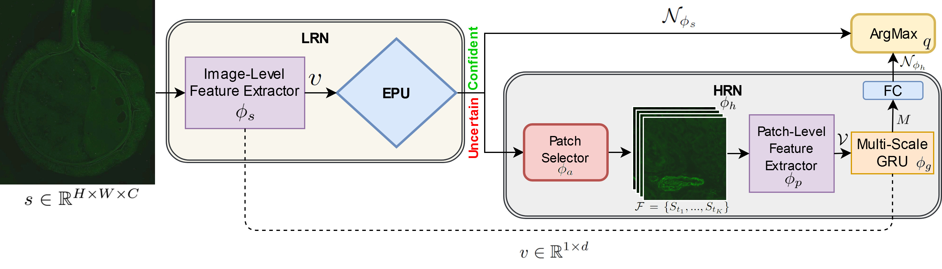
As illustrated in Figure 2, the aim of the SOS protocol is to avoid excessive high resolution patch-level processing for WSIs that can be classified confidently at the image-level. To this end, we train an EPU to serve as a controller that decides whether the LRN or HRN is used to classify a given WSI. We describe the details of these components and our optimization protocol below.
3.1 Model Framework
Low Resolution Network. Depending on the path chosen by the EPU, the LRN can serve as either a WSI classifier, or a feature extractor for the HRN. The LRN receives a downscaled WSI, , as input to a ResNet18 based feature extractor, , to compute a high level feature vector as:
| (1) |
where is the number of output channels from the penultimate layer of ResNet18 resnet.
Executive Processing Unit. The EPU is located at the terminal end of the LRN where it receives as input and estimates a set of class probabilities , where is number of WSI classes. To compute , we apply a linear transformation to followed by the softmax function :
| (2) |
where and are parameters learned by the network. The element with the highest value in is compared to a confidence threshold in the range to determine the flow of downstream operations.
As shown in Algorithm 1, the high confidence estimations immediately compute the class label using the function while the low confidence estimations trigger additional processing by the HRN . The details of the function are outlined below.

High Resolution Network. The HRN, , comprises three main subcomponents; a patch selector , a patch-level feature extractor , and a Gated Recurrent Unit (GRU) gru. The patch selector function is based on the stochastic hard attention mechanism proposed by Xu et al. attention. Specifically, the indices of elements in are treated as intermediate latent variables where is the set of high resolution patches derived from the full resolution WSI. We then estimate a Multinoulli distribution as a function of the image-level WSI features :
| (3) |
where and are parameters learned by the network. The indices of the highest elements in are used to sample the set of discriminate patches . The value of is limited by the maximum capacity of the GPU. In our experiments the upper limit of is . A set of patch-level feature vectors are then extracted by applying the function to each element in . The architecture of is a clone of . The reason for using a separate network to extract features from the high resolution patches is that CNNs are not robust to changes in scales snip. Thus, the objective of becomes:
| (4) |
The function receives and (via the residual connection to illustrated in Figure 2) as input and computes , where is a multi-scale representation of the WSI. The design of is similar to the late fusion multi-stream LSTM architecture described in patch_lstm, however, we substitute the LSTM for a GRU cell as they have been observed to achieve comparable performance at a lower computational cost gru_vs_lstm. The GRU cell, with hidden state , is first initialized with the image-level feature vector (), and subsequently receives a patch image feature vector in each time step for a total of time steps. The final state of the GRU cell is concatenated with to construct . Finally, we compute the class label as follows:
| (5) |
| (6) |
where and are parameters learned by the network and is the set of estimated class probabilities.
3.2 Optimization Protocol
Our model is trained by optimizing three loss terms: classification loss; paradoxical loss; and executive loss. During training, the EPU always triggers HRN processing to optimize the classification accuracy of both networks. During inference, the EPU uses the switch statement in Algorithm 1 to decide on a single path. We describe the details of our optimization protocol below.
Classification Loss. The classification loss is the summation of two cross entropy loss terms: a low resolution cross entropy loss ; and a high resolution cross entropy loss . The purpose of is to maximize the classification accuracy when inferring the class label from the LRN probability distribution :
| (7) |
where is the mini-batch size, is the class label, is the observed WSI, is a binary indication that is the ground truth label for , and is the probability that if predicted by the LRN. The purpose of is to maximize the classification accuracy when inferring from the HRN probability distribution . The term is the same as Equation 7, except we use probabilities in instead of to calculate the cross entropy loss. The loss is then computed as the sum of and .
Paradoxical Loss. The motivation of the paradoxical loss term is the assumption that, given is a multi-scale representation of image-level and patch-level features, access to more visual detail should never decrease the performance of the HRN. Thus, instances where the LRN performs better than the HRN during training should be viewed as undesirable and paradoxical. Under this assumption, we hypothesize that if the probability of the correct class is higher in than in , it must be due to either an overconfident LRN, or a suboptimal HRN. To deter these behaviors in our model we compute as follows:
| (8) |
where and are the estimated probabilities of the true class label by the LRN and HRN respectively.
Executive Loss. The Executive Loss is a weighted sum of two novel loss terms: a hesitation loss; and a hubristic loss. Its purpose is to calibrate both the confidence threshold (Algorithm 1) and the LRN confidence scores to achieve the optimal trade-off between efficiency and accuracy. This is crucial because confidence scores naturally produced by neural networks may not represent true probabilities cal. Intuitively, the hesitation loss and hubristic loss can be understood as the difference between the predicted probability value, and the value relative to that would have resulted in a correct action by the EPU.
The hesitation loss, , is the penalty incurred when there is a high degree of uncertainty in correct LRN predictions, resulting in redundant HRN processing. Specifically, this describes instances when: (a) the LRN predicts the correct class label, and (b) the predicted probability value is below the confidence threshold. To prevent our network from using the HRN excessively, we penalize correct LRN predictions when the probability value is below by computing as follows:
| (9) |
where is used to set the desired target above the confidence threshold, and is the binary indicator that is the correct label for observation .
The hubristic loss is the penalty incurred when the EPU’s decision to bypass correct HRN predictions is based on confidently incorrect predictions by the LRN. Specifically, this describes instances when: (a) the LRN predicts an incorrect class label; (b) the predicted probability value is above the confidence threshold; and (c) the HRN predicts the correct class label. To prevent this underutilization of the HRN, we penalize incorrect LRN predictions that are predicted with a probability value above by computing as:
| (10) |
where is binary indicator that is the correct class label for , and is the binary indicator that is the incorrect class label for .
Both and are then weighted to compute as:
| (11) |
where and are regularization terms that set the target speed/accuracy trade-off by controlling the influence of and on .
Final Objective Function. The final objective function is computed as the sum of , , and terms. By adding to the total network loss (rather than simply calibrating the threshold ), our network has the flexibility to improve EPU decision making by: (a) adjusting directly; and/or (b) modifying other network parameters to have the LRN regress confidence scores on the appropriate side of .
4 The Liver-Kidney-Stomach Dataset
| Set | Neg | AMA | SMA-V | SMA-T | Total |
|---|---|---|---|---|---|
| Train | |||||
| Test |
| Size | Resolution | Objective | Format |
|---|---|---|---|
| 300GB | TIFF |
The liver auto-antibody LKS screen is critical to the investigation of autoimmune liver disease ald; ald2, however, there are currently no public WSI datasets available for research. There are several reasons why the LKS classification task is ideal for evaluating dynamic multi-scale networks. Firstly, compared to public bright field microscopy WSI datasets, the increased sensitivity of the immunoflouresence assay allows for the observation of critical features at low resolution. Secondly, despite the increased sensitivity of IIF, high resolution may still be required to observe certain staining patterns, particularly when antibody concentrations are low. Finally, global structures captured at low resolution are essential for the classification of multi-tissue LKS WSIs. The fact that low resolution features are necessary, but not always sufficient, for LKS classification provides an ideal environment to validate the SOS protocol.
In collaboration with Sullivan Nicolaides Pathology, we constructed a novel LKS dataset from routine clinical samples. To prepare the LKS slides, sections of rodent kidney, stomach and liver tissue were prepared according to the schematic in Figure 1. Patient serum was incubated on the multi-tissue section and treated with fluorescein isothiocyanate (FITC) IgG conjugate. The slides were digitized using a monocolor camera and a x objective lens with a numerical aperture of . A team of trained medical scientists manually labelled the slides into one of four classes: Negative (Neg); Anti-Mitochondrial Antibodies (AMA); Vessel-Type Anti-Smooth Muscle Antibodies (SMA-V) and Tubule-Type Anti-Smooth Muscle Antibodies (SMA-T). The distribution of classes is provided in Table 1(a) and relevant meta-information is provided in Table 1(b).
5 Experiments
| TA% | IT(s) | RS | LP | CT | |||
|---|---|---|---|---|---|---|---|
| ✓ | ✓ | ||||||
| ✓ | ✓ | ||||||
| ✓ | ✓ | ||||||
| ✓ | |||||||
| ✓ |
| Fusion Method | TA% | IT(s) | RS | LP | CT |
|---|---|---|---|---|---|
| GRU | |||||
| Average Pool | |||||
| Max Pool |
The aim of the SOS protocol is to achieve rapid WSI classification without: (a) substantially increasing model size; or (b) compromising on classification accuracy. Thus, we validate the effectiveness of our method by analysing quantitative metrics for classification accuracy, model size, and processing speed. The design specifications for the SOS protocol, such as the number of patches processed at high resolution (), and the multi-image feature aggregation method (GRU), were determined by the outcomes of the ablation studies in Table 2. As described in Section 2, the existing approaches for WSI classification can be broadly grouped into: (a) Patch-Level; (b) Conventional Multi-Scale; and (c) Dynamic Multi-Scale methods. We assess the quantitative performance of our SOS protocol against each of these commonly used methods and additionally include image-level WSI classification performance for comparison (Tables 3 and 4). We also qualitatively analyze the outputs of our patch selection network to validate the effectiveness of our HRN (Figures 3 and 4).
5.1 Data Preprocessing
For computational efficiency, all WSIs were preprocessed into and prior to training and inference. To produce where , and ; we downscale the full resolution WSIs by a factor of . To produce , we segment full resolution WSIs into non-overlapping patches with the same dimensions as ; thus, the total number of patches per WSI is . Since ResNet18 resnet was designed to be used on tricolor image inputs, we modified the first convolutional layer to have single channel inputs to be compatible with these monocolor images.
| Method | TA% | RS | IT(s) | SB | LP |
|---|---|---|---|---|---|
| Image-Level | - | ||||
| Patch-Level | - | ||||
| Multi-Scale | - | ||||
| RDMS | 0.55 | ||||
| SOS (ours) | 0.94 |
5.2 Method Comparison
The details of each of the methods used for comparison are described below. All models were evaluated after training for epochs using a learning rate of .
Image-Level. The Image-Level method performs classification on single-scale image-level features. Specifically, we train a ResNet18 model resnet to directly compute the class label () from downscaled WSI () inputs. We optimize image-level classification by minimizing the cross entropy loss for ground truth and predicted class probabilities.
Patch-Level. The Patch-Level method performs classification on single-scale patch-level features. The network architecture is essentially the same as the proposed model; however, we remove the residual connection to image-level features. Thus, only high resolution features from the set of patches are used to classify the WSI. We optimize patch-level classification by minimizing the cross entropy loss for ground truth and predicted class probabilities.
Conventional Multi-Scale. The Conventional Multi-Scale method performs classification on multi-scale image-level and patch-level features. The design of the Multi-Scale method is similar to the Patch-Level network; however, we restore the residual connection to image-level features as shown in Figure 2. Thus, features from both low resolution and high resolution image scales are used to classify each WSI. We optimize multi-scale classification by minimizing the cross entropy loss for ground truth and predicted class probabilities. In this paper, we refer to this method as Multi-Scale.
Dynamic Multi-Scale. The Dynamic Multi-Scale method is based on the Reinforced Auto-Zoom Net (RAZN) framework proposed by Dong et al. razn. Specifically, we remove the switch statement (Algorithm 1) from the EPU and attach a policy network, based on the ResNet architecture, to the front end of our model to decide whether to use the LRN or the HRN for WSI classification. Since RAZN is designed for WSI segmentation tasks, we modify the reward function to be suitable for LKS classification as follows:
| (12) |
where , represents the policy action to use the LRN or HRN respectively. Thus, when then the reward is positive if , and negative if . We then optimize the network using the policy gradient method described in razn. We refer to this method as Reinforced Dynamic Multi-Scale (RDMS).
5.3 Quantitative Evaluation
Processing Speed. Processing speed is evaluated using Inference Time (IT) and Speed Boost (SB) metrics. The IT is a raw measurement of inference time (in seconds) on the test dataset. SB indicates the factor by which inference time is reduced relative to the baseline model. The model used as the baseline for processing speed is the conventional Multi-Scale model. The reason for selecting this model as the baseline is because it achieved the highest accuracy among the static classification models. Thus, it defines the baseline speed at which the highest accuracy can be achieved without adapting the resolution used to process each WSI.
Model Size. The model size is evaluated using the Relative Size (RS) metric. The RS metric indicates the relative increase in size compared to the simple image-level ResNet18 classifier used as the backbone in all our multi-scale methods e.g. an RS of indicates that the model has twice as many parameters as the simple ResNet18 classifier.
Classification Accuracy. The classification accuracy is evaluated using the Total Accuracy (TA) metric. However, since the majority of samples in the dataset are negative, the TA does not provide an adequate measure of classification performance on individual classes. To assess individual class performance, we provide the F1 score (F1), Precision (PR), Recall (RE), and Specificity (SP) for each of the four WSI classes in Table 4.
| Method | F1 | PR | RE | SP |
|---|---|---|---|---|
| Image-Level | ||||
| Patch-Level | ||||
| Multi-Scale | ||||
| RDMS | ||||
| SOS (ours) |
| Method | F1 | PR | RE | SP |
|---|---|---|---|---|
| Image-Level | ||||
| Patch-Level | ||||
| Multi-Scale | ||||
| RDMS | ||||
| SOS (ours) |
| Method | F1 | PR | RE | SP |
|---|---|---|---|---|
| Image-Level | ||||
| Patch-Level | ||||
| Multi-Scale | ||||
| RDMS | ||||
| SOS (ours) |
| Method | F1 | PR | RE | SP |
|---|---|---|---|---|
| Image-Level | ||||
| Patch-Level | ||||
| Multi-Scale | ||||
| RDMS | ||||
| SOS (ours) |
6 Discussion

The results in Table 3 indicate that our proposed method was able to reduce inference time by a factor of while improving classification accuracy compared to the conventional multi-scale approach. The improved classification accuracy was unexpected because the multi-scale network processes low resolution contextual features and high resolution local features for every WSI while our network only uses single-scale low resolution features for the majority of test samples. We suspect that training our model to use LRN features for patch selection and classification may explain the improved accuracy as it has been shown that jointly learning the tasks of detection and classification have a beneficial effect on model performance joint_task.
The RDMS method was also shown to improve accuracy and reduce inference time. However, as shown in Table 3, adding the additional policy network has introduced significantly more parameters than our proposed method. The limitations of using RDMS for classification tasks are demonstrated clearly by the LP of 0.55; meaning only of samples in the test dataset were classified at low resolution compared to our . The fact that our model still achieved a higher accuracy when processing fewer samples at high resolution indicates that RDMS is using the HRN excessively. This behavior was expected because the policy reward in RDMS (Equation 12) is always zero unless the “zoom” (HRN processing) action is sampled. This means there is an incentive to utilize HRN processing whenever the incurred loss is lower than the LRN prediction i.e. . However, in classification tasks, a lower cross entropy loss is not a perfect estimate of classification accuracy because the LRN may still reliably predict the correct class label. In our method, we encourage the network to maximize the use of LRN for classification in these cases by minimizing (Equation 9). Thus, we could classify WSIs significantly faster than RDMS without compromising on classification accuracy.
Figure 4 provides examples of sampled patches for each of the WSI classes. At low resolution, it is virtually impossible to resolve the fine smooth muscle actin fibres in SMA-T and SMA-V patches. The staining of actin fibres is an essential diagnostic feature of smooth muscle antibodies ald. The inability to resolve these fibres at low resolution likely explains why the F1 scores for these classes are substantially lower with the Image-Level classifier than with the Multi-Scale, RDMS and SOS methods; which all incorporate high resolution WSI features (Table 4). The Patch-Level method also has access to the high resolution WSI features; however, without any spatial context features from the low resolution WSI, it obtained the lowest classification accuracy of all tested methods (Table 3).
While the HRN clearly improves the accuracy of our model, the hard patch attention mechanism often selects patches containing no tissue at all (Figure 3). The selection of undesirable patches likely explains why average and max pooling methods do not perform as well as the gated recurrent unit for aggregating multi-image features (Table 2) — as recurrent neural networks are known to be more robust to noisy WSI patches patch_lstm.
From the ablation studies in Table 2, it is clear that reducing the number of patches processed by the HRN will have an adverse effect on classification accuracy. Omitting the paradoxical loss () during training also results in a significant drop in classification accuracy. The paradoxical loss is used to prevent overconfident estimates by the LRN; without it, the model becomes biased towards classifying examples at low resolution (as indicated by the LP of ). A smaller reduction in classification accuracy is also observed when the executive loss term () was omitted during training. The executive loss term helps regulate the network to regress class probability estimates on the appropriate side of the decision boundary. Without the executive loss, class probabilities can be estimated without feedback on how they affected EPU decisions; which can result in the suboptimal image scale being selected to classify a WSI.
7 Conclusion
In this paper, we show that it is possible to reduce inference time in WSI classification tasks, without compromising on accuracy, by restricting high resolution patch-based processing to cases that cannot be classified confidently at low resolution. The effectiveness of our proposed SOS protocol is demonstrated on the LKS dataset; which presents the challenging task of finding the optimal trade-off between low resolution WSI processing and patch-based processing. To evaluate the generalizability of the proposed framework, in future works, we will perform experiments on a variety of IIF WSI datasets that are being assembled in collaboration with Sullivan Nicolaides Pathology.
8 Acknowledgements
This project has been funded by Sullivan Nicolaides Pathology and the Australian Research Council (ARC) Linkage Project [Grant number LP160101797].
References
- (1) The cancer genome atlas. http://cancergenome.nih.gov.
- (2) Guilherme Aresta, Teresa Araújo, Scotty Kwok, Sai Saketh Chennamsetty, Mohammed Safwan, Varghese Alex, Bahram Marami, Marcel Prastawa, Monica Chan, Michael Donovan, et al. Bach: Grand challenge on breast cancer histology images. Medical image analysis, 2019.
- (3) Peter Bandi, Oscar Geessink, Quirine Manson, Marcory Van Dijk, Maschenka Balkenhol, Meyke Hermsen, Babak Ehteshami Bejnordi, Byungjae Lee, Kyunghyun Paeng, Aoxiao Zhong, et al. From detection of individual metastases to classification of lymph node status at the patient level: the camelyon17 challenge. IEEE transactions on medical imaging, 38(2):550–560, 2018.
- (4) Aïcha BenTaieb and Ghassan Hamarneh. Predicting cancer with a recurrent visual attention model for histopathology images. In International Conference on Medical Image Computing and Computer-Assisted Intervention, pages 129–137. Springer, 2018.
- (5) Tad T Brunye, Patricia A Carney, Kimberly H Allison, Linda G Shapiro, Donald L Weaver, and Joann G Elmore. Eye movements as an index of pathologist visual expertise: a pilot study. PloS one, 9(8):e103447, 2014.
- (6) Kyunghyun Cho, Bart Van Merriënboer, Caglar Gulcehre, Dzmitry Bahdanau, Fethi Bougares, Holger Schwenk, and Yoshua Bengio. Learning phrase representations using rnn encoder-decoder for statistical machine translation. arXiv preprint arXiv:1406.1078, 2014.
- (7) Junyoung Chung, Caglar Gulcehre, KyungHyun Cho, and Yoshua Bengio. Empirical evaluation of gated recurrent neural networks on sequence modeling. arXiv preprint arXiv:1412.3555, 2014.
- (8) Jia Deng, Wei Dong, Richard Socher, Li-Jia Li, Kai Li, and Li Fei-Fei. Imagenet: A large-scale hierarchical image database. In 2009 IEEE conference on computer vision and pattern recognition, pages 248–255. Ieee, 2009.
- (9) Nanqing Dong, Michael Kampffmeyer, Xiaodan Liang, Zeya Wang, Wei Dai, and Eric Xing. Reinforced auto-zoom net: Towards accurate and fast breast cancer segmentation in whole-slide images. In Deep Learning in Medical Image Analysis and Multimodal Learning for Clinical Decision Support, pages 317–325. Springer, 2018.
- (10) Nikolaos K Gatselis, Kalliopi Zachou, George K Koukoulis, and George N Dalekos. Autoimmune hepatitis, one disease with many faces: etiopathogenetic, clinico-laboratory and histological characteristics. World journal of gastroenterology: WJG, 21(1):60, 2015.
- (11) Mohsen Ghafoorian, Nico Karssemeijer, Tom Heskes, Mayra Bergkamp, Joost Wissink, Jiri Obels, Karlijn Keizer, Frank-Erik de Leeuw, Bram van Ginneken, Elena Marchiori, et al. Deep multi-scale location-aware 3d convolutional neural networks for automated detection of lacunes of presumed vascular origin. NeuroImage: Clinical, 14:391–399, 2017.
- (12) Chuan Guo, Geoff Pleiss, Yu Sun, and Kilian Q Weinberger. On calibration of modern neural networks. In Proceedings of the 34th International Conference on Machine Learning-Volume 70, pages 1321–1330. JMLR. org, 2017.
- (13) Zichao Guo, Hong Liu, Haomiao Ni, Xiangdong Wang, Mingming Su, Wei Guo, Kuansong Wang, Taijiao Jiang, and Yueliang Qian. A fast and refined cancer regions segmentation framework in whole-slide breast pathological images. Scientific reports, 9(1):882, 2019.
- (14) Kaiming He, Xiangyu Zhang, Shaoqing Ren, and Jian Sun. Deep residual learning for image recognition. In Proceedings of the IEEE conference on computer vision and pattern recognition, pages 770–778, 2016.
- (15) Sepp Hochreiter and Jürgen Schmidhuber. Long short-term memory. Neural computation, 9(8):1735–1780, 1997.
- (16) Le Hou, Dimitris Samaras, Tahsin M Kurc, Yi Gao, James E Davis, and Joel H Saltz. Patch-based convolutional neural network for whole slide tissue image classification. In Proceedings of the IEEE Conference on Computer Vision and Pattern Recognition, pages 2424–2433, 2016.
- (17) Geert Litjens, Peter Bandi, Babak Ehteshami Bejnordi, Oscar Geessink, Maschenka Balkenhol, Peter Bult, Altuna Halilovic, Meyke Hermsen, Rob van de Loo, Rob Vogels, et al. 1399 h&e-stained sentinel lymph node sections of breast cancer patients: the camelyon dataset. GigaScience, 7(6):giy065, 2018.
- (18) Geert Litjens, Thijs Kooi, Babak Ehteshami Bejnordi, Arnaud Arindra Adiyoso Setio, Francesco Ciompi, Mohsen Ghafoorian, Jeroen Awm Van Der Laak, Bram Van Ginneken, and Clara I Sánchez. A survey on deep learning in medical image analysis. Medical image analysis, 42:60–88, 2017.
- (19) Kevis-Kokitsi Maninis, Ilija Radosavovic, and Iasonas Kokkinos. Attentive single-tasking of multiple tasks. In Proceedings of the IEEE Conference on Computer Vision and Pattern Recognition, pages 1851–1860, 2019.
- (20) Pedro HO Pinheiro and Ronan Collobert. Recurrent convolutional neural networks for scene labeling. In 31st International Conference on Machine Learning (ICML), number CONF, 2014.
- (21) Bharat Singh and Larry S Davis. An analysis of scale invariance in object detection snip. In Proceedings of the IEEE conference on computer vision and pattern recognition, pages 3578–3587, 2018.
- (22) Korsuk Sirinukunwattana, Nasullah Khalid Alham, Clare Verrill, and Jens Rittscher. Improving whole slide segmentation through visual context-a systematic study. In International Conference on Medical Image Computing and Computer-Assisted Intervention, pages 192–200. Springer, 2018.
- (23) Richard S Sutton, David A McAllester, Satinder P Singh, and Yishay Mansour. Policy gradient methods for reinforcement learning with function approximation. In Advances in neural information processing systems, pages 1057–1063, 2000.
- (24) Ban-Hock Toh. Diagnostic autoantibodies for autoimmune liver diseases. Clinical & translational immunology, 6(5):e139, 2017.
- (25) Hiroki Tokunaga, Yuki Teramoto, Akihiko Yoshizawa, and Ryoma Bise. Adaptive weighting multi-field-of-view cnn for semantic segmentation in pathology. In Proceedings of the IEEE Conference on Computer Vision and Pattern Recognition, pages 12597–12606, 2019.
- (26) Kelvin Xu, Jimmy Ba, Ryan Kiros, Kyunghyun Cho, Aaron Courville, Ruslan Salakhudinov, Rich Zemel, and Yoshua Bengio. Show, attend and tell: Neural image caption generation with visual attention. In International conference on machine learning, pages 2048–2057, 2015.
- (27) Yan Xu, Zhipeng Jia, Yuqing Ai, Fang Zhang, Maode Lai, I Eric, and Chao Chang. Deep convolutional activation features for large scale brain tumor histopathology image classification and segmentation. In 2015 IEEE international conference on acoustics, speech and signal processing (ICASSP), pages 947–951. IEEE, 2015.