跳到论文正文
W Papers独立论文阅读器 arXiv:2003.04758 论文正文 计算阅读时间 · 0%
引用这篇论文根据当前论文元数据生成,正式投稿前建议核对。


License: arXiv.org perpetual non-exclusive license
arXiv:2003.04758v1 [cs.IT] 09 Mar 2020

Performance Analysis of NOMA Uplink Networks under Statistical QoS Delay Constraints

Mouktar Bello1 , Wenjuan Yu 2, Arsenia Chorti1 and Leila Musavian4 Affiliation: 1ETIS UMR8051, CY Université, ENSEA, CNRS, F-95000, Cergy, France Affiliation: 25GIC, Institute of Communication Systems, University of Surrey, Guildford, GU2 7XH, UK Affiliation: 4School of Computer Science and Electronic Engineering, University of Essex, Colchester, CO4 3SQ, UK
Abstract

In the fifth generation and beyond (B5G), delay constraints emerge as a topic of particular interest, e.g. for ultra-reliable low latency communications (URLLC) such as autonomous vehicles and enhanced reality. In this paper, we study the performance of a two-user uplink NOMA network under statistical quality of service (QoS) delay constraints, captured through each user’s effective capacity (EC). We propose novel closed-form expressions for the EC of the NOMA users and show that in the high signal to noise ratio (SNR) region, the “strong” NOMA user has a limited EC, assuming the same delay constraint as the “weak” user. We demonstrate that for the weak user, OMA achieves higher EC than NOMA at small values of the transmit SNR, while NOMA outperforms OMA in terms of EC at high SNRs. On the other hand, for the strong user the opposite is true, i.e., NOMA achieves higher EC than OMA at small SNRs, while OMA becomes more beneficial at high SNRs. This result raises the question of introducing “adaptive” OMA / NOMA policies, based jointly on the users’ delay constraints as well as on the available transmit power.

Index Terms: 
NOMA, QoS, low latency, effective capacity, B5G.

I Introduction

Non-orthogonal multiple access (NOMA) schemes have attracted a lot of attention recently, allowing multiple users to be served simultaneously with enhanced spectral efficiency; it is known that the boundary of achievable rate pairs (in the case of two users) using NOMA is outside the capacity region achievable with orthogonal multiple access (OMA) techniques [1] or other schemes [2]. Superior achievable rates are attainable through the use of superposition coding at the transmitter and of successive interference cancellation (SIC) at the receiver [3, 4]. The SIC receiver decodes multi-user signals with descending received signal power and subtracts the decoded signal(s) from the received superimposed signal, so as to improve the signal-to-interference ratio. The process is repeated until the signal of interest is decoded. In uplink NOMA networks, the strongest user’s signal is decoded first (as opposed to downlink NOMA networks in which the inverse order is applied).

Besides, in a number of emerging applications, delay quality of service (QoS) becomes increasingly important, e.g., ultra reliable low latency communication (URLLC) systems. Furthermore, in future wireless networks, users are expected to necessitate flexible delay guarantees for achieving different service requirements. In order to satisfy diverse delay requirements, a simple and flexible delay QoS model is imperative to be applied and investigated. In this respect, the effective capacity (EC) theory can be employed [5],[6] [7], with EC denoting the maximum constant arrival rate which can be served by a given service process, while guaranteeing the required statistical delay provisioning. We studied the delay-constrained communications for a downlink NOMA network in [4] and with secrecy constraints [8] in [9]. The present analysis complements [4], focusing on uplink transmissions. NOMA, as a more spectrum-efficient technique, is considered to be promising for supporting the massive number of devices to access the uplink connections. Hence, we believe that it is important to investigate the delay-constrained achievable rate for an uplink NOMA network.

In this paper, we provide a performance evaluation of the uplink transmission for a two-user NOMA network under delay constraints, captured through the users’ ECs. We note that the EC is a QoS aware data-link layer metric [6], that captures the achievable rate under a delay violation probability threshold.

In this work, we first derive novel closed-form expressions for the ECs of both users; we then provide four Lemmas for the asymptotic performance of the network with NOMA and OMA. The conclusions drawn are supported by an extensive set of simulations. The paper is organized as follows. In Section II we investigate the EC of a two user uplink NOMA system under the delay QoS constraints. Simulation results are given in Section III, followed by conclusions in Section IV.

II Effective Capacity of Two-user NOMA Uplink Network

Assume a two-user NOMA uplink network with users U1 and U2 in a Rayleigh block fading propagation channel, with respective channel gains during a transmission block denoted by |h1|2<|h2|2|h_{1}|^{2}<|h_{2}|^{2}. The users transmit corresponding symbols S1,S2S_{1},S_{2} respectively, with power 𝔼[|Si|2]=Pi,i=1,2\mathbb{E}[|S_{i}|^{2}]=P_{i},i=1,2 and the total power PT=∑i=12Pi=1P_{T}=\sum_{i=1}^{2}{P_{i}}=1. Here, PiP_{i} is the power coefficient for the user ii and normalized transmission powers are assumed[10]. The received superimposed signal can be expressed as[11]

Z=∑i=12Pi​hi​Si+w,Z=\sum_{i=1}^{2}\sqrt{P_{i}}h_{i}S_{i}+w, (1)

where ww denotes a zero mean circularly symmetric complex Gaussian random variable with variance σ2\sigma^{2}. The receiver will first decode the symbol of the strong user treating the transmission of the weak as interference. After decoding it, the receiver will suppress it from ZZ and decode the signal of the weak user. Following the SIC principle and denoting by ρ=1σ2\rho=\frac{1}{\sigma^{2}} the transmit SNR, the achievable rates, in b/s/Hz, for user Ui,i=1,2{}_{i},i=1,2, is expressed as: [12]

Ri=log2⁡[1+ρ​Pi​|hi|21+ρ​∑l=1i−1Pl​|hl|2].R_{i}=\log_{2}\left[1+\frac{\rho P_{i}|h_{i}|^{2}}{1+\rho\sum_{l=1}^{i-1}P_{l}|h_{l}|^{2}}\right]. (2)

To clarify further, let θi\theta_{i} be the statistical delay QoS exponent of the ii-th user, and assume that the service process satisfies the Gärtner-Ellis theorem [6]. The delay exponent θi\theta_{i} captures how strict the delay constraint is [6]. A slower decay rate can be represented by a smaller θi\theta_{i}, which indicates that the system is more delay tolerant, while a larger θi\theta_{i} corresponds to a system with more stringent QoS requirements. Applying the EC theory in a uplink NOMA with two users, the ii-th user’s EC over a block-fading channel, is defined as:

Eci=−1θi​Tf​B​ln⁡(𝔼⁡[e−θi​Tf​B​Ri])(in b/s/Hz),\displaystyle E_{c}^{i}=-\frac{1}{\theta_{i}T_{{f}}B}\ln\left(\mathbb{E}\left[e^{-\theta_{i}T_{\text{f}}BR_{i}}\right]\right)\quad\left(\text{in b/s/Hz}\right), (3)

where TfT_{f} is the fading-block length, BB is the bandwidth and 𝔼⁡[⋅]\mathbb{E}\left[\cdot\right] denotes expectation over the channel gains. By inserting RiR_{i} into (3), we obtain the following expression for the EC of the ii-th user

Eci\displaystyle E_{c}^{i} =\displaystyle= 1βi​log2⁡(𝔼⁡[(1+ρ​Pi​|hi|21+ρ​∑l=1i−1Pl​|hl|2)βi])\displaystyle\frac{1}{\beta_{i}}\log_{2}\left(\mathbb{E}\left[(1+\frac{\rho P_{i}|h_{i}|^{2}}{1+\rho\sum_{l=1}^{i-1}P_{l}|h_{l}|^{2}})^{\beta_{i}}\right]\right) (4)

where βi=−θi​Tf​Bln⁡2\beta_{i}=-\frac{\theta_{i}T_{f}B}{\ln{2}}, i=1,2i=1,2, is the normalized (negative) QoS exponent.

II-A ECs in a Two-user NOMA Uplink Network

For the ordering of the channel gains we make use of the theory of order statistics in the following analysis [13].

Assuming a Rayleigh wireless environment, the channel gains, denoted by xi=|hi|2,i=1,2x_{i}=|h_{i}|^{2},i=1,2, are exponentially distributed with probability density function (PDF) and cumulative density function (CDF) respectively given by f⁡(xi)=e−xif(x_{i})=e^{-x_{i}}, F⁡(xi)=1−e−xiF(x_{i})=1-e^{-x_{i}}.

Then, according to order statistics[13], the ordered channel gains have respective PDFs fi:2(xi),i=1,2f_{i:2}(x_{i}),i=1,2, and joint PDF f⁡(x1,x2)f(x_{1},x_{2}) that are expressed as

f1:2(x1)\displaystyle f_{1:2}(x_{1}) =2​e−2​x1,\displaystyle=2e^{-2x_{1}}, (5)
f2:2(x2)\displaystyle f_{2:2}(x_{2}) =2​e−x2​(1−e−x2),\displaystyle=2e^{-x_{2}}\left(1-e^{-x_{2}}\right), (6)
f⁡(x1,x2)\displaystyle f(x_{1},x_{2}) =2​e−x1​e−x2.\displaystyle=2e^{-x_{1}}e^{-x_{2}}. (7)

As a result, the EC of User 1, denoted by Ec1E_{c}^{1} is expressed as

Ec1\displaystyle E_{c}^{1} =\displaystyle= 1β1​log2⁡(𝔼⁡[(1+ρ​P1​x1)β1])\displaystyle\frac{1}{\beta_{1}}\log_{2}(\mathbb{E}[(1+\rho P_{1}x_{1})^{\beta_{1}}]) (8)
=\displaystyle= 1β1log2(∫0∞(1+ρP1x1)β1f1:2(x1)dx1)\displaystyle\frac{1}{\beta_{1}}\log_{2}\Big(\int_{0}^{\infty}(1+\rho P_{1}x_{1})^{\beta_{1}}f_{{1:2}}(x_{1})dx_{1}\Big)
=\displaystyle= 1β1​log2⁡(2P1​ρ×U⁡(1,2+β1,2ρ​P1)).\displaystyle\frac{1}{\beta_{1}}\log_{2}\Big(\frac{2}{P_{1}\rho}\times U\left(1,2+\beta_{1},\frac{2}{\rho P_{1}}\right)\Big).

where U⁡(⋅,⋅,⋅)U(\cdot,\cdot,\cdot) denotes the confluent hypergeometric function [4]. On the other hand, the EC of the User 2 is evaluated as

Ec2\displaystyle E_{c}^{2} =1β2​log2⁡(𝔼⁡[(1+ρ​P2​x21+ρ​P1​x1)β2])\displaystyle=\frac{1}{\beta_{2}}\log_{2}\left(\mathbb{E}\left[\left(1+\frac{\rho P_{2}x_{2}}{1+\rho P_{1}x_{1}}\right)^{\beta_{2}}\right]\right)
=1β2​log2⁡(∫0∞∫x1∞(1+ρ​P2​x21+ρ​P1​x1)β2​f​(x1,x2)​d​x2​d​x1)\displaystyle=\frac{1}{\beta_{2}}\log_{2}\left(\int_{0}^{\infty}\!\!\!\!\int_{x_{1}}^{\infty}\!\!\!\!\Big(1+\frac{\rho P_{2}x_{2}}{1+\rho P_{1}x_{1}}\Big)^{\beta_{2}}f(x_{1},x_{2})dx_{2}dx_{1}\right)
=1β2​log2⁡(2​P21−β2​(ρ​P2)β2​e1ρ​P2​e−(P1−P2)ρ​P2)\displaystyle=\frac{1}{\beta_{2}}\log_{2}\Big(2P_{2}^{1-\beta_{2}}(\rho P_{2})^{\beta_{2}}e^{\frac{1}{\rho P_{2}}}e^{-\frac{(P_{1}-P_{2})}{\rho P_{2}}}\Big)
+1β2​log2⁡(∑j=0−β2(−β2j)​(ρ​P1)j×∑k=0∞(−1)k​(P2−P1)kk!​(1+j+k)CLOSE\displaystyle+\frac{1}{\beta_{2}}\log_{2}\Bigg(\sum_{j=0}^{-\beta_{2}}\binom{-\beta_{2}}{j}(\rho P_{1})^{j}\times\sum_{k=0}^{\infty}\frac{(-1)^{k}(P_{2}-P_{1})^{k}}{k!(1+j+k)}
×[Γ[2+β2+j+k,1ρ​P2]\displaystyle\times\Big[\Gamma[2+\beta_{2}+j+k,\frac{1}{\rho P_{2}}]
−(ρP2)−1−j−kΓ[1+β2,1ρ​P2]]),\displaystyle-(\rho P_{2})^{-1-j-k}\Gamma[1+\beta_{2},\frac{1}{\rho P_{2}}]\Big]\Bigg), (9)

with Γ⁡(⋅,⋅)\Gamma(\cdot,\cdot) denoting the incomplete Gamma function [4].

The proof for deriving Ec1E_{c}^{1} is omitted due to space limitations while for Ec2E_{c}^{2} is provided in Appendix I.

In order to perform a comparative performance analysis, here we provide the achievable data rates for a two-user OMA network, denoted by R~i,i=1,2\widetilde{R}_{i},i=1,2, given as

R~i=12log2(1+ρPT|hi|2),i=1,2\widetilde{R}_{i}=\frac{1}{2}\log_{2}\Big(1+\rho P_{T}|h_{i}|^{2}\Big),i=1,2 (10)

Note that 12\frac{1}{2} is due to the equal allocation of resources to both users. The corresponding expressions are obtained for the ECs of both users in a OMA network, denoted by E~ci\widetilde{E}_{c}^{i}, given as

E~ci\displaystyle\widetilde{E}_{c}^{i} =1βi​log2⁡(𝔼⁡[(1+ρ​PT​|hi|2)βi2])\displaystyle=\frac{1}{\beta_{i}}\log_{2}\Big(\mathbb{E}\Big[(1+\rho P_{T}|h_{i}|^{2})^{\frac{\beta_{i}}{2}}\Big]\Big)
i.e,\displaystyle i.e, (11)
E~c1=1β1​log2⁡(2ρ×U⁡(1,2+β12,2ρ))\displaystyle\widetilde{E}_{c}^{1}=\frac{1}{\beta_{1}}\log_{2}\left(\frac{2}{\rho}\times U\left(1,2+\frac{\beta_{1}}{2},\frac{2}{\rho}\right)\right)
E~c2=1β2​log2⁡(2ρ​∑k=01(1k)​(−1)k×U⁡(1,2+β22,1+kρ))\displaystyle\!\!\!\!\!\widetilde{E}_{c}^{2}=\frac{1}{\beta_{2}}\log_{2}\left(\frac{2}{\rho}\sum_{k=0}^{1}\binom{1}{k}(-1)^{k}\times U\left(1,2+\frac{\beta_{2}}{2},\frac{1+k}{\rho}\right)\right)

The proof is omitted due to space limitations.

II-B Asymptotic Analysis

We first perform an asymptotic analysis with respect to the SNR. Our results are summarized in Lemma 1.

Lemma 1

In the low and high SNR regimes, respectively, the following conclusions hold:

  1. 1.

    When ρ→0\rho\rightarrow 0, then, Ec1→0E_{c}^{1}\rightarrow 0, Ec2→0E_{c}^{2}\rightarrow 0, E~c1→0\widetilde{E}_{c}^{1}\rightarrow 0, E~c2→0\widetilde{E}_{c}^{2}\rightarrow 0, Ec1−E~c1→0E_{c}^{1}-\widetilde{E}_{c}^{1}\rightarrow 0, Ec2−E~c2→0E_{c}^{2}-\widetilde{E}_{c}^{2}\rightarrow 0;

  2. 2.

    When ρ→+∞\rho\rightarrow+\infty, then Ec1→+∞E_{c}^{1}\rightarrow+\infty, Ec2→1β2​log2⁡(𝔼⁡[(1+P2​|h2|2P1​|h1|2)β2])E_{c}^{2}\rightarrow\frac{1}{\beta_{2}}\log_{2}\left(\mathbb{E}\left[\left(1+\frac{P_{2}|h_{2}|^{2}}{P_{1}|h_{1}|^{2}}\right)^{\beta_{2}}\right]\right), E~c1→+∞\widetilde{E}_{c}^{1}\rightarrow+\infty, E~c2→+∞\widetilde{E}_{c}^{2}\rightarrow+\infty, Ec1−E~c1→+∞E_{c}^{1}-\widetilde{E}_{c}^{1}\rightarrow+\infty, Ec2−E~c2→−∞E_{c}^{2}-\widetilde{E}_{c}^{2}\rightarrow-\infty.

Proof:

: The proof is provided in Appendix II.∎

Lemma 1 indicates that the ECs of both users are vanishingly small at low values of ρ\rho, irrespective of employing NOMA or OMA. On the other hand, at high SNRs, we notice that the EC of the strong user with NOMA is limited to a finite value. On the contrary, for the weaker user, when ρ>>1\rho>>1, its achievable EC in the NOMA uplink increases without bound. This is the exact opposite of the downlink scenario, where it is the weaker user which is limited in terms of EC, when ρ>>1\rho>>1 [4].

Now, the question is how the ECs evolve with ρ\rho between the two asymptotic regimes. To answer this question and to further analyze the impact of ρ\rho on the individual EC, we look at the derivatives with the respect of ρ\rho [4].

Lemma 2

For the EC of the User 1, in a two-user uplink network the following hold:

  1. 1.

    ∂Ec1∂ρ≥0\frac{\partial E_{c}^{1}}{\partial\rho}\geq 0 and ∂E~c1∂ρ≥0\frac{\partial\widetilde{E}_{c}^{1}}{\partial\rho}\geq 0, ∀ρ\forall\rho;

  2. 2.

    When ρ→0\rho\rightarrow 0, then limρ→0(∂(Ec1−E~c1)∂ρ)=P1−12ln⁡2​𝔼​[|h1|2]\lim\limits_{\rho\rightarrow 0}(\frac{\partial(E_{c}^{1}-\widetilde{E}_{c}^{1})}{\partial\rho})=\frac{P_{1}-\frac{1}{2}}{\ln 2}\mathbb{E}[|h_{1}|^{2}];

  3. 3.

    When ρ>>1\rho>>1, then ∂(Ec1−E~c1)∂ρ≈12​ρ​ln⁡2≥0\frac{\partial(E_{c}^{1}-\widetilde{E}_{c}^{1})}{\partial\rho}\approx\frac{1}{2\rho\ln 2}\geq 0 and it approaches 00 when ρ→∞\rho\rightarrow\infty.

Proof:

: The proof is provided in Appendix III.∎

Lemma 2 indicates that for User 1, when the transmit SNR ρ\rho is very small, the EC with OMA increases faster than the EC with NOMA. On the other hand, Lemma 2 shows that when the transmit SNR is very large, the EC with NOMA increases faster than with OMA.

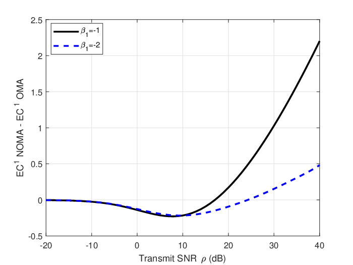
Combining Lemma 2 and Lemma 1, we can conclude that, Ec1−E~c1E_{c}^{1}-\widetilde{E}_{c}^{1} starts at vanishingly small value, first decreases, and subsequently increases to ∞\infty at a gradually reducing speed. This means that for the weaker user, OMA achieves higher EC than NOMA at small values of the transmit SNR ρ\rho. At high values of ρ\rho, NOMA becomes more beneficial for the weak user. Finally, when ρ→∞\rho\rightarrow\infty the performance gain of NOMA over OMA reaches a constant value in the case of User 1.

Lemma 3

For the EC of the User 2, in a two-user uplink network the following hold:

  1. 1.

    ∂Ec2∂ρ≥0\frac{\partial E_{c}^{2}}{\partial\rho}\geq 0 and ∂E~c2∂ρ≥0\frac{\partial\widetilde{E}_{c}^{2}}{\partial\rho}\geq 0, ∀ρ\forall\rho;

  2. 2.

    When ρ→0\rho\rightarrow 0, then limρ→0(∂(Ec2−E~c2)∂ρ)=P22​ln⁡2​𝔼​[|h2|2]\lim\limits_{\rho\rightarrow 0}(\frac{\partial(E_{c}^{2}-\widetilde{E}_{c}^{2})}{\partial\rho})=\frac{P_{2}}{2\ln 2}\mathbb{E}[|h_{2}|^{2}]

  3. 3.

    When ρ>>1\rho>>1, then ∂(Ec2−E~c2)∂ρ≈−12​ln⁡2​1ρ<0\frac{\partial(E_{c}^{2}-\widetilde{E}_{c}^{2})}{\partial\rho}\approx-\frac{1}{2\ln 2}\frac{1}{\rho}<0 and it approaches 0 when ρ→∞\rho\rightarrow\infty.

Proof:

The proof is provided in Appendix IV.∎

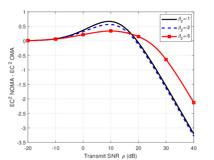
Lemma 3 indicates that, for User 2, when the transmit SNR ρ\rho is very small, the uplink EC with NOMA increases faster than that with OMA. On the other hand, when the transmit SNR is very large, the uplink EC with OMA increases faster than that with NOMA. Combining Lemma 3 and Lemma 1, we can conclude that, Ec2−E~c2E_{c}^{2}-\widetilde{E}_{c}^{2} starts at an initial vanishingly small value, first increases, and subsequently decreases to −∞-\infty with a gradually diminishing rate. This means that for the stronger user, NOMA achieves higher EC than OMA at small values of the transmit SNR ρ\rho. At high values of ρ\rho, OMA becomes more beneficial for the strong user. Finally, when ρ→∞\rho\rightarrow\infty the performance gain of OMA over NOMA reaches a constant value, for the stronger user.

Finally, we investigate the sum ECs when using OMA and NOMA, denoted by VNV_{N} and VOV_{O},

VN\displaystyle V_{N} =\displaystyle= Ec1+Ec2,\displaystyle E_{c}^{1}+E_{c}^{2}, (12)
VO\displaystyle V_{O} =\displaystyle= E~c1+E~c2.\displaystyle\widetilde{E}_{c}^{1}+\widetilde{E}_{c}^{2}. (13)

Our conclusions are drawn in Lemma 4.

Lemma 4

For the sum EC with NOMA, denoted by VNV_{N}, and with OMA, denoted by VOV_{O}, in a two-user uplink network, the following hold:

  1. 1.

    ∂VN∂ρ≥0\frac{\partial V_{N}}{\partial\rho}\geq 0 and ∂VO∂ρ≥0\frac{\partial V_{O}}{\partial\rho}\geq 0, ∀ρ\forall\rho;

  2. 2.

    When ρ→0\rho\rightarrow 0, VN→0V_{N}\rightarrow 0, limρ→0(∂VN∂ρ)=P1ln⁡2​𝔼​[|h1|2]+P2ln⁡2​𝔼​[|h2|2]≥0\lim\limits_{\rho\rightarrow 0}(\frac{\partial V_{N}}{\partial\rho})=\frac{P_{1}}{\ln 2}\mathbb{E}[|h_{1}|^{2}]+\frac{P_{2}}{\ln 2}\mathbb{E}[|h_{2}|^{2}]\geq 0, and VO→0V_{O}\rightarrow 0, limρ→0(∂VO∂ρ)=P12​ln⁡2​𝔼​[|h1|2]+P22​ln⁡2​𝔼​[|h2|2]≥0\lim\limits_{\rho\rightarrow 0}(\frac{\partial V_{O}}{\partial\rho})=\frac{P_{1}}{2\ln 2}\mathbb{E}[|h_{1}|^{2}]+\frac{P_{2}}{2\ln 2}\mathbb{E}[|h_{2}|^{2}]\geq 0;

  3. 3.

    When ρ>>1\rho>>1, VN→∞V_{N}\rightarrow\infty, limρ→∞(∂VN∂ρ)=0\lim\limits_{\rho\rightarrow\infty}(\frac{\partial V_{N}}{\partial\rho})=0, and VO→∞V_{O}\rightarrow\infty, limρ→∞(∂VO∂ρ)=0\lim\limits_{\rho\rightarrow\infty}(\frac{\partial V_{O}}{\partial\rho})=0.

Proof:

The proof is provided in Appendix V.∎

Lemma 4 indicates that when NOMA is applied, the sum EC has a constant increasing rate at small value of the transmit SNR ρ\rho that depends on the average of the channel power gains and the allocated power coefficients. A similar conclusion is reached when using OMA. On the other hand, when ρ>>1\rho>>1, Lemma 4 indicates that the rate at which the sum ECs increase reaches a plateau, both in the case of NOMA and OMA.

III Numerical Results

In this section, the Lemmas presented in Section II will be validated through Monte Carlo simulations. We consider a two user uplink NOMA system, with the following settings: normalized transmission powers for both users, P1=0.2P_{1}=0.2, P2=0.8P_{2}=0.8, normalized delay exponent β1=β2=−1\beta_{1}=\beta_{2}=-1 for both users, unless otherwise stated.

In Fig. 1 the ECs of the two-user uplink NOMA and OMA networks are depicted versus the transmit SNR. We note that for the weak user, OMA is advantageous than NOMA for low transmit SNRs, and NOMA is advantageous OMA at high transmit SNRs. Reverse conclusions can be drawn for the strong user. We notice also that the EC of the strong user converges at high SNRs. This provides numerical validation for Lemma 1.

Refer to caption
Fig. 1: Ec1E_{c}^{1}, Ec2E_{c}^{2}in a two-user NOMA uplink network compared to Ecs of two users OMA, versus ρ\rho

Figs. 2 and 3, show respectively the EC of User 1 and User 2, versus the transmit SNR, for different values of β1=β2=β\beta_{1}=\beta_{2}=\beta. When the delay constraints become more stringent, i.e., β\beta decreases (equivalently, θ\theta increases), the individual link-layer rates in NOMA decrease, for both users.

Refer to caption
Fig. 2: Ec1E_{c}^{1} versus the transmit SNR, for several delays.
Refer to caption
Fig. 3: Ec2E_{c}^{2} versus the transmit SNR ρ\rho for several delays.

In Fig. 4, the ECs of the strong and weak users are depicted across different SNR values, (ρ∈{1,10,30,40,50}\rho\in\{1,10,30,40,50\} dB, as functions of the (negative) normalized delay exponent, for NOMA and OMA scenarios. We notice that the EC of each user is identical for NOMA and OMA, for small and large values of the normalized delay exponent. And with the transmit SNR ρ\rho increasing, the EC increases for both users.

Refer to caption
Fig. 4: Ec1E_{c}^{1} and Ec2E_{c}^{2} in a two-user NOMA compared to ECs of two users OMA, versus normalized delay β\beta, for different values of ρ\rho.

Fig. 5 shows the difference of the EC in NOMA and the EC in OMA of the weak user. This curve starts initially at zero, then decreases to a certain minimum and starts increasing at the high values of transmit SNR. This confirms Lemma 2. When the delay is equal to −1-1, we see that for ρ∈[−20,15]\rho\in[-20,15] dB, the difference values are negative, indicating that OMA outperforms NOMA in this range. But when ρ>15\rho>15 dB, the values are positive, i.e., NOMA offers better link-layer rates. However, the particular ranges depend not only on the delay exponents but also on the power allocation coefficients. By increasing the transmission power of the weak user and reducing the transmission power of the strong user, we notice that the range is reduced. That range expands when we do the inverse. Also, when the delay becomes more stringent, e.g., β1\beta_{1}=β2\beta_{2}=-2, the zero crossing moves from 1515 to 2525 dB.

Refer to caption
Fig. 5: Ec1−E~c1E_{c}^{1}-\tilde{E}_{c}^{1} versus ρ\rho, for several values of the normalized delay exponent.

Figure 6 shows the difference of the EC in NOMA and the EC in OMA for the strong user. This curve starts initially at zero, then increases to a certain maximum and starts decreasing without bound at high values of the transmit SNR. This confirms Lemma 3. We note that the maximum of these curves decreases when the delay becomes more stringent.

Refer to caption
Fig. 6: Ec2−E~c2E_{c}^{2}-\tilde{E}_{c}^{2} versus ρ\rho, for various normalized delay exponent.

To investigate the impact of ρ\rho on the performance of the total link-layer rate for the two-user system, in Fig. 7 the plots for VNV_{N} in NOMA and VOV_{O} in OMA, versus the transmit SNR are depicted for various delay exponents. The curves demonstrate that for both NOMA and OMA, the total EC for the two users starts at the initial value of 0 and then increases with the transmit SNR, as outlined in Lemma 4. When ρ\rho is very small, the total link-layer rate for the two user in NOMA, VNV_{N}, increases faster than VOV_{O} in OMA. On the contrary, with the increase of the transmit SNR, VOV_{O} becomes gradually higher than VNV_{N}. At very high values of the transmit SNR, the gap between the sum EC with NOMA and OMA increases further. Finally, when the delay becomes more stringent, the sum EC of both NOMA and OMA decreases.

Refer to caption
Fig. 7: VNV_{N} and VOV_{O} versus ρ\rho, for several values of normalized delay exponent.

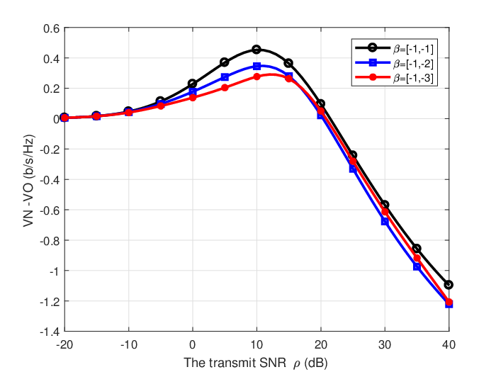
Finally, Figs 8 and 9 depict the sum ECs versus ρ\rho, for several values of the (negative) normalized delay exponent. In Fig. 8, the delay of the strong user is fixed, while the delay exponent of the weak user varies. It is shown that in this case, the highest delay QoS (i.e., the smallest negative normalized delay exponent) of the weak user corresponds to the highest gap between the sum ECs VN−VOV_{N}-V_{O}. On the other hand, when the delay of the weak user is fixed, Fig. 9 shows that the smallest delay Qos (i.e., the highest negative normalized delay exponent) for the strong user corresponds to the largest gap in VN−VOV_{N}-V_{O}.

Refer to caption
Fig. 8: VNV_{N} - VOV_{O} versus ρ\rho for various normalized delay.
Refer to caption
Fig. 9: VNV_{N} - VOV_{O} versus ρ\rho for various normalized delay.

The curve of VN−VOV_{N}-V_{O} starts at zero, increases to a maximum, and returns to negative values. The transition to zero is at around ρ\rho = 25, and ρ\rho =20 respectively for the figures 8 and 9. That means from 0 to 25dB (20dB in the Figure 9), the total link-layer rate of NOMA is higher than the OMA one. And when ρ\rho becomes larger than this transition point, the total link-layer rate of OMA outperforms the NOMA one.

IV Conclusions and Future Work

The concept of the EC enabled us to study the achievable data-link layer rates when the delay QoS guarantees are in place in the form of delay exponents. We investigated the EC for the uplink of a two-user NOMA network, assuming a Rayleigh block fading channel. We derived novel closed-form expressions for the ECs of the two users and provided a comparison between NOMA and OMA. In NOMA networks, we showed that the ECs of both users decrease as the delay constraints become stringent. On the other hand, at high transmit SNRs, the EC of the weak user can surpass the EC of the strong user, as the latter is limited due to interference. This provides the possibility of switching between NOMA and OMA according to the individual users’ delay constraints and transmit powers. In future work, the impact of user pairing will also be investigated.

Appendix I

For the second user, we have:

Ec2\displaystyle E_{c}^{2} =\displaystyle= 1β2​log2⁡(2​∫0∞(ρ​P21+ρ​P1​x1)β2​e−x1CLOSE\displaystyle\frac{1}{\beta_{2}}\log_{2}\Bigg(2\int_{0}^{\infty}(\frac{\rho P_{2}}{1+\rho P_{1}x_{1}})^{\beta_{2}}e^{-x_{1}}
×\displaystyle\times OPEN∫x1∞(1+ρ​P1​x1ρ​P2+x2)β2​e−x2​d​x2​d​x1).\displaystyle\int_{x_{1}}^{\infty}\Big(\frac{1+\rho P_{1}x_{1}}{\rho P_{2}}+x_{2}\Big)^{\beta_{2}}e^{-x_{2}}dx_{2}dx_{1}\Bigg).

Set z=1+ρ​P1​x1ρ​P2+x2z=\frac{1+\rho P_{1}x_{1}}{\rho P_{2}}+x_{2}, which means we have x2=z−1+ρ​P1​x1ρ​P2x_{2}=z-\frac{1+\rho P_{1}x_{1}}{\rho P_{2}} and d​x2=d​zdx_{2}=dz. Then,

Ec2\displaystyle E_{c}^{2}\!\!\!\! =\displaystyle= 1β2​log2⁡(2​e1ρ​P2​∫0∞(ρ​P21+ρ​P1​x1)β2​e−x1​eP1​x1P2CLOSE\displaystyle\!\!\!\!\frac{1}{\beta_{2}}\log_{2}\Big(2e^{\frac{1}{\rho P_{2}}}\int_{0}^{\infty}(\frac{\rho P_{2}}{1+\rho P_{1}x_{1}})^{\beta_{2}}e^{-x_{1}}e^{\frac{P_{1}x_{1}}{P_{2}}}
OPEN∫1+ρ​x1ρ​P2∞zβ2​e−z​𝑑z​d​x1)\displaystyle\!\!\!\!\int_{\frac{1+\rho x_{1}}{\rho P_{2}}}^{\infty}z^{\beta_{2}}e^{-z}dzdx_{1}\Big)
=\displaystyle= 1β2​log2⁡(2​(ρ​P2)β22​e12​ρ​P2​∫0∞(1+ρ​P1​x1)−β2CLOSE\displaystyle\!\!\!\!\frac{1}{\beta_{2}}\log_{2}\Bigg(2(\rho P_{2})^{\frac{\beta_{2}}{2}}e^{\frac{1}{2\rho P_{2}}}\int_{0}^{\infty}(1+\rho P_{1}x_{1})^{-\beta_{2}}
OPEN(1+ρ​x1)β22​e(2​P1−2​P2−1)​x12​P2​[𝐖β22,1+β22​(1+ρ​x1ρ​P2)]​d​x1)\displaystyle\!\!\!\!\!\!\!\!(1+\rho x_{1})^{\frac{\beta_{2}}{2}}e^{\frac{(2P_{1}-2P_{2}-1)x_{1}}{2P_{2}}}\Big[\mathbf{W}_{\frac{\beta_{2}}{2},\frac{1+\beta_{2}}{2}}(\frac{1+\rho x_{1}}{\rho P_{2}})\Big]dx_{1}\Bigg)
=\displaystyle= 1β2​log2⁡(2​P2​(ρ​P2)β2​e1ρ​P2​e−(P1−P2)ρ​P2CLOSE\displaystyle\!\!\!\!\frac{1}{\beta_{2}}\log_{2}\Bigg(2P_{2}(\rho P_{2})^{\beta_{2}}e^{\frac{1}{\rho P_{2}}}e^{-\frac{(P_{1}-P_{2})}{\rho P_{2}}}
OPEN∫1ρ​P2∞P2−β2​(1+ρ​P1​y)−β2​e(P1−P2)​y​Γ​(1+β2,y)​𝑑y),\displaystyle\!\!\!\!\int_{\frac{1}{\rho P_{2}}}^{\infty}P_{2}^{-\beta_{2}}(1+\rho P_{1}y)^{-\beta_{2}}e^{(P_{1}-P_{2})y}\Gamma(1+\beta_{2},y)dy\Bigg),

where 𝐖\mathbf{W} is the Whittaker W function.

Using the binomial expansion, we have (1+ρ​P1​y)−β2=∑j=0−β2(−β2j)​(ρ​P1​y)j(1+\rho P_{1}y)^{-\beta_{2}}=\sum_{j=0}^{-\beta_{2}}\binom{-\beta_{2}}{j}(\rho P_{1}y)^{j}. and we get the expression given in (9).

Appendix II

By inserting ρ→0\rho\rightarrow 0 into (8) and (9), we get 1) of Lemma 1, i.e.,

limρ→0(Ec1−E~c1)=1β1​log2⁡(𝔼⁡[(1+ρ​P1​|h1|2)β2]𝔼⁡[(1+ρ​|h1|2)β22])=0,\lim\limits_{\rho\rightarrow 0}(E_{c}^{1}-\widetilde{E}_{c}^{1})=\frac{1}{\beta_{1}}\log_{2}(\frac{\mathbb{E}[(1+\rho P_{1}|h_{1}|^{2})^{\beta_{2}}]}{\mathbb{E}[(1+\rho|h_{1}|^{2})^{\frac{\beta_{2}}{2}}]})=0,
limρ→0(Ec2−E~c2)=1β2​log2⁡(𝔼⁡[(1+ρ​P2​|h2|21+ρ​P1​|h1|2)β2]𝔼⁡[(1+ρ​|h2|2)β22])=0.\lim\limits_{\rho\rightarrow 0}(E_{c}^{2}-\widetilde{E}_{c}^{2})=\frac{1}{\beta_{2}}\log_{2}\left(\frac{\mathbb{E}[(1+\frac{\rho P_{2}|h_{2}|^{2}}{1+\rho P_{1}|h_{1}|^{2}})^{\beta_{2}}]}{\mathbb{E}[(1+\rho|h_{2}|^{2})^{\frac{\beta_{2}}{2}}]}\right)=0.

In the same way, by inserting ρ→∞\rho\rightarrow\infty into (8) and (9), we get 2) in Lemma 1, given below.

limρ→∞Ec2\displaystyle\lim\limits_{\rho\rightarrow\infty}E_{c}^{2} →1β2​log2⁡(𝔼⁡[(1+P2​|h2|2P1​|h1|2)β2]),\displaystyle\rightarrow\frac{1}{\beta_{2}}\log_{2}(\mathbb{E}[(1+\frac{P_{2}|h_{2}|^{2}}{P_{1}|h_{1}|^{2}})^{\beta_{2}}]),
limρ→∞(Ec1−E~c1)\displaystyle\lim\limits_{\rho\rightarrow\infty}(E_{c}^{1}-\widetilde{E}_{c}^{1}) =1β1​log2⁡(ρβ12​𝔼⁡[(1ρ+P1​|h1|2)β2]𝔼⁡[(1ρ+|h1|2)β22])=∞,\displaystyle=\frac{1}{\beta_{1}}\log_{2}(\rho^{\frac{\beta_{1}}{2}}\frac{\mathbb{E}[(\frac{1}{\rho}+P_{1}|h_{1}|^{2})^{\beta_{2}}]}{\mathbb{E}[(\frac{1}{\rho}+|h_{1}|^{2})^{\frac{\beta_{2}}{2}}]})=\infty,
limρ→∞(Ec2−E~c2)\displaystyle\lim\limits_{\rho\rightarrow\infty}(E_{c}^{2}-\widetilde{E}_{c}^{2}) =1β2​log2⁡(𝔼⁡[(1ρ+P1​|h1|2+P2​|h2|21ρ+P1​|h1|2)β2]ρβ22​𝔼​[(1ρ+|h2|2)β22])=−∞.\displaystyle=\frac{1}{\beta_{2}}\log_{2}(\frac{\mathbb{E}[(\frac{\frac{1}{\rho}+P_{1}|h_{1}|^{2}+P_{2}|h_{2}|^{2}}{\frac{1}{\rho}+P_{1}|h_{1}|^{2}})^{\beta_{2}}]}{\rho^{\frac{\beta_{2}}{2}}\mathbb{E}[(\frac{1}{\rho}+|h_{2}|^{2})^{\frac{\beta_{2}}{2}}]})=\!\!-\infty.

Appendix III

To analyze the trends of Ec1E_{c}^{1} and E~c1\widetilde{E}_{c}^{1} with respect to ρ\rho, we start with

∂Ec1∂ρ\displaystyle\frac{\partial E_{c}^{1}}{\partial\rho} =1β1​ln⁡2​(𝔼⁡[(1+ρ​P1​|h1|2)β1])′𝔼⁡[(1+ρ​P1​|h1|2)β1]\displaystyle=\frac{1}{\beta_{1}\ln 2}\frac{\Big(\mathbb{E}[(1+\rho P_{1}|h_{1}|^{2})^{\beta_{1}}]\Big)^{\prime}}{\mathbb{E}[(1+\rho P_{1}|h_{1}|^{2})^{\beta_{1}}]}
=P1ln⁡2​𝔼⁡[|h1|2​(1+ρ​P1​|h1|2)β1−1]𝔼⁡[(1+ρ​P1​|h1|2)β1]≥0.\displaystyle=\frac{P_{1}}{\ln 2}\frac{\mathbb{E}[|h_{1}|^{2}(1+\rho P_{1}|h_{1}|^{2})^{\beta_{1}-1}]}{\mathbb{E}[(1+\rho P_{1}|h_{1}|^{2})^{\beta_{1}}]}\geq 0.

Similarly, for user 1 in OMA we have

∂E~c1∂ρ\displaystyle\frac{\partial\widetilde{E}_{c}^{1}}{\partial\rho} =1β1​ln⁡2​(𝔼⁡[(1+ρ​|h1|2)β12])′𝔼⁡[(1+ρ​|h1|2)β12]\displaystyle=\frac{1}{\beta_{1}\ln 2}\frac{\Big(\mathbb{E}[(1+\rho|h_{1}|^{2})^{\frac{\beta_{1}}{2}}]\Big)^{\prime}}{\mathbb{E}[(1+\rho|h_{1}|^{2})^{\frac{\beta_{1}}{2}}]}
=12​ln⁡2​𝔼⁡[|h1|2​(1+ρ​|h1|2)β12−1]𝔼⁡[(1+ρ​|h1|2)β12]≥0.\displaystyle=\frac{1}{2\ln 2}\frac{\mathbb{E}[|h_{1}|^{2}(1+\rho|h_{1}|^{2})^{\frac{\beta_{1}}{2}-1}]}{\mathbb{E}[(1+\rho|h_{1}|^{2})^{\frac{\beta_{1}}{2}}]}\geq 0.

Then, we get that

∂(Ec1−E~c1)∂ρ\displaystyle\frac{\partial(E_{c}^{1}-\widetilde{E}_{c}^{1})}{\partial\rho} =P1ln⁡2​𝔼⁡[|h1|2​(1+ρ​P1​|h1|2)β1−1]𝔼⁡[(1+ρ​P1​|h1|2)β1]\displaystyle=\frac{P_{1}}{\ln 2}\frac{\mathbb{E}[|h_{1}|^{2}(1+\rho P_{1}|h_{1}|^{2})^{\beta_{1}-1}]}{\mathbb{E}[(1+\rho P_{1}|h_{1}|^{2})^{\beta_{1}}]}
−12​ln⁡2​𝔼⁡[|h1|2​(1+ρ​|h1|2)β12−1]𝔼⁡[(1+ρ​|h1|2)β12],\displaystyle-\frac{1}{2\ln 2}\frac{\mathbb{E}[|h_{1}|^{2}(1+\rho|h_{1}|^{2})^{\frac{\beta_{1}}{2}-1}]}{\mathbb{E}[(1+\rho|h_{1}|^{2})^{\frac{\beta_{1}}{2}}]},

and limρ→0(∂(Ec1−E~c1)∂ρ)=(P1−12)ln⁡2​𝔼​[|h1|2]≤0\lim\limits_{\rho\rightarrow 0}(\frac{\partial(E_{c}^{1}-\widetilde{E}_{c}^{1})}{\partial\rho})=\frac{(P_{1}-\frac{1}{2})}{\ln 2}\mathbb{E}[|h_{1}|^{2}]\leq 0. When ρ>>1\rho>>1, we have

OPEN∂(Ec1−E~c1)∂ρ)\displaystyle\frac{\partial(E_{c}^{1}-\widetilde{E}_{c}^{1})}{\partial\rho}) =P1ln⁡2​𝔼⁡[|h1|2​(ρ​P1​|h1|2)β1−1]𝔼⁡[(ρ​P1​|h1|2)β1]\displaystyle=\frac{P_{1}}{\ln 2}\frac{\mathbb{E}[|h_{1}|^{2}(\rho P_{1}|h_{1}|^{2})^{\beta_{1}-1}]}{\mathbb{E}[(\rho P_{1}|h_{1}|^{2})^{\beta_{1}}]}
−12​ln⁡2​𝔼⁡[|h1|2​(ρ​|h1|2)β12−1]𝔼⁡[(ρ​|h1|2)β12]=12​ρ​ln⁡2≥0.\displaystyle-\frac{1}{2\ln 2}\frac{\mathbb{E}[|h_{1}|^{2}(\rho|h_{1}|^{2})^{\frac{\beta_{1}}{2}-1}]}{\mathbb{E}[(\rho|h_{1}|^{2})^{\frac{\beta_{1}}{2}}]}=\frac{1}{2\rho\ln 2}\geq 0.

When ρ→∞\rho\rightarrow\infty, this term approaches 0.

Appendix IV

Ec2=1β2​log2⁡(𝔼⁡[(1+ρ​P2​|h2|21+ρ​P1​|h1|2)β2]), and E_{c}^{2}=\frac{1}{\beta_{2}}\log_{2}(\mathbb{E}[(1+\frac{\rho P_{2}|h_{2}|^{2}}{1+\rho P_{1}|h_{1}|^{2}})^{\beta_{2}}]),\text{ and }

∂Ec2∂ρ\displaystyle\frac{\partial E_{c}^{2}}{\partial\rho} =1β2​ln⁡2​(𝔼⁡[(1+ρ​P2​|h2|21+ρ​P1​|h1|2)β2])′𝔼⁡[(1+ρ​P2​|h2|21+ρ​P1​|h1|2)β2]\displaystyle=\frac{1}{\beta_{2}\ln 2}\frac{\Big(\mathbb{E}[(1+\frac{\rho P_{2}|h_{2}|^{2}}{1+\rho P_{1}|h_{1}|^{2}})^{\beta_{2}}]\Big)^{\prime}}{\mathbb{E}[(1+\frac{\rho P_{2}|h_{2}|^{2}}{1+\rho P_{1}|h_{1}|^{2}})^{\beta_{2}}]}
=1ln⁡2​𝔼⁡[P2​|h2|2(1+ρ​P1​|h1|2)2​(1+ρ​P2​|h2|21+ρ​P1​|h1|2)β2−1]𝔼⁡[(1+ρ​P2​|h2|21+ρ​P1​|h1|2)β2]≥0.\displaystyle=\!\!\frac{1}{\ln 2}\frac{\mathbb{E}[\frac{P_{2}|h_{2}|^{2}}{(1+\rho P_{1}|h_{1}|^{2})^{2}}(1+\frac{\rho P_{2}|h_{2}|^{2}}{1+\rho P_{1}|h_{1}|^{2}})^{\beta_{2}-1}]}{\mathbb{E}[(1+\frac{\rho P_{2}|h_{2}|^{2}}{1+\rho P_{1}|h_{1}|^{2}})^{\beta_{2}}]}\geq 0.

In the same way, for the user 2 in OMA, we have

∂E~c2∂ρ\displaystyle\frac{\partial\widetilde{E}_{c}^{2}}{\partial\rho} =1β2​ln⁡2​(𝔼⁡[(1+ρ​|h2|2)β22])′𝔼⁡[(1+ρ​|h2|2)β22]\displaystyle=\frac{1}{\beta_{2}\ln 2}\frac{\Big(\mathbb{E}[(1+\rho|h_{2}|^{2})^{\frac{\beta_{2}}{2}}]\Big)^{\prime}}{\mathbb{E}[(1+\rho|h_{2}|^{2})^{\frac{\beta_{2}}{2}}]}
=12​ln⁡2​𝔼⁡[|h2|2​(1+ρ​|h2|2)β22−1]𝔼⁡[(1+ρ​|h2|2)β22]≥0, and\displaystyle=\frac{1}{2\ln 2}\frac{\mathbb{E}[|h_{2}|^{2}(1+\rho|h_{2}|^{2})^{\frac{\beta_{2}}{2}-1}]}{\mathbb{E}[(1+\rho|h_{2}|^{2})^{\frac{\beta_{2}}{2}}]}\geq 0,\text{ and}
∂(Ec2−E~c2)∂ρ\displaystyle\frac{\partial(E_{c}^{2}-\widetilde{E}_{c}^{2})}{\partial\rho} =1ln⁡2​𝔼⁡[P2​|h2|2(1+ρ​P1​|h1|2)2​(1+ρ​P2​|h2|21+ρ​P1​|h1|2)β2−1]𝔼⁡[(1+ρ​P2​|h2|21+ρ​P1​|h1|2)β2]\displaystyle=\frac{1}{\ln 2}\frac{\mathbb{E}[\frac{P_{2}|h_{2}|^{2}}{(1+\rho P_{1}|h_{1}|^{2})^{2}}(1+\frac{\rho P_{2}|h_{2}|^{2}}{1+\rho P_{1}|h_{1}|^{2}})^{\beta_{2}-1}]}{\mathbb{E}[(1+\frac{\rho P_{2}|h_{2}|^{2}}{1+\rho P_{1}|h_{1}|^{2}})^{\beta_{2}}]}
−12​ln⁡2​𝔼⁡[|h2|2​(1+ρ​|h2|2)β22−1]𝔼⁡[(1+ρ​|h2|2)β22].\displaystyle-\frac{1}{2\ln 2}\frac{\mathbb{E}[|h_{2}|^{2}(1+\rho|h_{2}|^{2})^{\frac{\beta_{2}}{2}-1}]}{\mathbb{E}[(1+\rho|h_{2}|^{2})^{\frac{\beta_{2}}{2}}]}.

When ρ→0\rho\rightarrow 0, we have that limρ→0(∂(Ec2−E~c2)∂ρ)=(P2−12)ln⁡2​𝔼​[|h2|2]\lim\limits_{\rho\rightarrow 0}(\frac{\partial(E_{c}^{2}-\widetilde{E}_{c}^{2})}{\partial\rho})=\frac{(P_{2}-\frac{1}{2})}{\ln 2}\mathbb{E}[|h_{2}|^{2}]. When ρ\rho is very large,

∂(Ec2−E~c2)∂ρ=𝔼⁡[P2​|h2|2ρ2​(1ρ+P1​|h1|2)2​(1+ρρ​(P2​|h2|2)(1ρ+P1​|h1|2))β2−1]ln⁡2​𝔼​[(1+ρρ​P2​|h2|2(1ρ+P1​|h1|2))β2]\displaystyle\frac{\partial(E_{c}^{2}-\widetilde{E}_{c}^{2})}{\partial\rho}=\frac{\mathbb{E}[\frac{P_{2}|h_{2}|^{2}}{\rho^{2}(\frac{1}{\rho}+P_{1}|h_{1}|^{2})^{2}}(1+\frac{\rho}{\rho}\frac{(P_{2}|h_{2}|^{2})}{(\frac{1}{\rho}+P_{1}|h_{1}|^{2})})^{\beta_{2}-1}]}{\ln 2\mathbb{E}[(1+\frac{\rho}{\rho}\frac{P_{2}|h_{2}|^{2}}{(\frac{1}{\rho}+P_{1}|h_{1}|^{2})})^{\beta_{2}}]}
−12​ln⁡2​1ρ​𝔼⁡[|h2|2​(1ρ+|h2|2)β22−1]𝔼⁡[(1ρ+|h2|2)β22]\displaystyle\qquad\qquad-\frac{1}{2\ln 2}\frac{1}{\rho}\frac{\mathbb{E}[|h_{2}|^{2}(\frac{1}{\rho}+|h_{2}|^{2})^{\frac{\beta_{2}}{2}-1}]}{\mathbb{E}[(\frac{1}{\rho}+|h_{2}|^{2})^{\frac{\beta_{2}}{2}}]}
=𝔼⁡[P2​|h2|2ρ2​(P1​|h1|2)2​(1+P2​|h2|2P1​|h1|2)β2−1]ln⁡2​𝔼​[(1+P2​|h2|2P1​|h1|2)β2]−12​ln⁡2​1ρ​𝔼⁡[(|h2|2)β22]𝔼⁡[(|h2|2)β22]\displaystyle=\!\!\frac{\mathbb{E}[\frac{P_{2}|h_{2}|^{2}}{\rho^{2}(P_{1}|h_{1}|^{2})^{2}}(1+\frac{P_{2}|h_{2}|^{2}}{P_{1}|h_{1}|^{2}})^{\beta_{2}-1}]}{\ln 2\mathbb{E}[(1+\frac{P_{2}|h_{2}|^{2}}{P_{1}|h_{1}|^{2}})^{\beta_{2}}]}-\frac{1}{2\ln 2}\frac{1}{\rho}\frac{\mathbb{E}[(|h_{2}|^{2})^{\frac{\beta_{2}}{2}}]}{\mathbb{E}[(|h_{2}|^{2})^{\frac{\beta_{2}}{2}}]}
=P2ρ2​P12​𝔼⁡[|h2|2(|h1|2)2​(1+P2​|h2|2P1​|h1|2)β2−1]ln⁡2​𝔼​[(1+P2​|h2|2P1​|h1|2)β2]−12​ln⁡2​1ρ\displaystyle=\frac{P_{2}}{\rho^{2}P_{1}^{2}}\frac{\mathbb{E}[\frac{|h_{2}|^{2}}{(|h_{1}|^{2})^{2}}(1+\frac{P_{2}|h_{2}|^{2}}{P_{1}|h_{1}|^{2}})^{\beta_{2}-1}]}{\ln 2\mathbb{E}[(1+\frac{P_{2}|h_{2}|^{2}}{P_{1}|h_{1}|^{2}})^{\beta_{2}}]}-\frac{1}{2\ln 2}\frac{1}{\rho}
=P2P12​ln⁡2​A−12​ln⁡2​ρρ2,\displaystyle=\frac{\frac{P_{2}}{P_{1}^{2}\ln 2}A-\frac{1}{2\ln 2}\rho}{\rho^{2}},

where A=𝔼⁡[|h2|2(|h1|2)2​(1+P2​|h2|2P1​|h1|2)β2−1]𝔼⁡[(1+P2​|h2|2P1​|h1|2)β2]A=\frac{\mathbb{E}[\frac{|h_{2}|^{2}}{(|h_{1}|^{2})^{2}}(1+\frac{P_{2}|h_{2}|^{2}}{P_{1}|h_{1}|^{2}})^{\beta_{2}-1}]}{\mathbb{E}[(1+\frac{P_{2}|h_{2}|^{2}}{P_{1}|h_{1}|^{2}})^{\beta_{2}}]}, unrelated to ρ\rho. Hence, when ρ\rho is very large, ∂(Ec2−E~c2)∂ρ\frac{\partial(E_{c}^{2}-\widetilde{E}_{c}^{2})}{\partial\rho} can be approximated by −12​ln⁡2​1ρ-\frac{1}{2\ln 2}\frac{1}{\rho}, and it gradually approaches 0 when ρ→∞\rho\rightarrow\infty.

Appendix V

Note that VN=Ec1+Ec2V_{N}=E_{c}^{1}+E_{c}^{2}. By using Lemma 1, we have limρ→0(VN)=0\lim\limits_{\rho\rightarrow 0}(V_{N})=0 and limρ→∞(VN)=∞\lim\limits_{\rho\rightarrow\infty}(V_{N})=\infty. Then, we get that

∂VN∂ρ\displaystyle\frac{\partial V_{N}}{\partial\rho} =∂(Ec1+Ec2)∂ρ=P1ln⁡2​𝔼⁡[|h1|2​(1+ρ​P1​|h1|2)β1−1]𝔼⁡[(1+ρ​P1​|h1|2)β1]\displaystyle=\frac{\partial(E_{c}^{1}+E_{c}^{2})}{\partial\rho}=\frac{P_{1}}{\ln 2}\frac{\mathbb{E}[|h_{1}|^{2}(1+\rho P_{1}|h_{1}|^{2})^{\beta_{1}-1}]}{\mathbb{E}[(1+\rho P_{1}|h_{1}|^{2})^{\beta_{1}}]}
+1ln⁡2​𝔼⁡[P2​|h2|2(1+ρ​P1​|h1|2)2​(1+ρ​P2​|h2|21+ρ​P1​|h1|2)β2−1]𝔼⁡[(1+ρ​P2​|h2|21+ρ​P1​|h1|2)β2]≥0.\displaystyle+\frac{1}{\ln 2}\frac{\mathbb{E}[\frac{P_{2}|h_{2}|^{2}}{(1+\rho P_{1}|h_{1}|^{2})^{2}}(1+\frac{\rho P_{2}|h_{2}|^{2}}{1+\rho P_{1}|h_{1}|^{2}})^{\beta_{2}-1}]}{\mathbb{E}[(1+\frac{\rho P_{2}|h_{2}|^{2}}{1+\rho P_{1}|h_{1}|^{2}})^{\beta_{2}}]}\geq 0.

When ρ→0\rho\rightarrow 0, we have limρ→0(∂VN∂ρ)=P1ln⁡2​𝔼​[|h1|2]+P2ln⁡2​𝔼​[|h2|2]\lim\limits_{\rho\rightarrow 0}(\frac{\partial V_{N}}{\partial\rho})=\frac{P_{1}}{\ln 2}\mathbb{E}[|h_{1}|^{2}]+\frac{P_{2}}{\ln 2}\mathbb{E}[|h_{2}|^{2}]. When ρ→∞\rho\rightarrow\infty, we get that

limρ→∞∂VN∂ρ=1ρ​ln⁡2+𝔼⁡[P2​|h2|2(P1​|h1|2)2​(1+P2​|h2|2P1​|h1|2)β2−1]ρ2​ln⁡2​𝔼​[(1+P2​|h2|2P1​|h1|2)β2]=0.\lim\limits_{\rho\rightarrow\infty}\frac{\partial V_{N}}{\partial\rho}=\frac{1}{\rho\ln 2}+\frac{\mathbb{E}[\frac{P_{2}|h_{2}|^{2}}{(P_{1}|h_{1}|^{2})^{2}}(1+\frac{P_{2}|h_{2}|^{2}}{P_{1}|h_{1}|^{2}})^{\beta_{2}-1}]}{\rho^{2}\ln 2\mathbb{E}[(1+\frac{P_{2}|h_{2}|^{2}}{P_{1}|h_{1}|^{2}})^{\beta_{2}}]}\!\!=\!\!0.

For VOV_{O} in the case of OMA, we note that VO=E~c1+E~c2V_{O}=\widetilde{E}_{c}^{1}+\widetilde{E}_{c}^{2}. By using Lemma 1, we have limρ→0(V0)=0\lim\limits_{\rho\rightarrow 0}(V_{0})=0 and limρ→∞(V0)=∞\lim\limits_{\rho\rightarrow\infty}(V_{0})=\infty. Then,

∂V0∂ρ\displaystyle\frac{\partial V_{0}}{\partial\rho} =∂(E~c1+E~c2)∂ρ=12​ln⁡2​𝔼⁡[|h1|2​(1+ρ​|h1|2)β12−1]𝔼⁡[(1+ρ​|h1|2)β12]\displaystyle=\frac{\partial(\widetilde{E}_{c}^{1}+\widetilde{E}_{c}^{2})}{\partial\rho}=\frac{1}{2\ln 2}\frac{\mathbb{E}[|h_{1}|^{2}(1+\rho|h_{1}|^{2})^{\frac{\beta_{1}}{2}-1}]}{\mathbb{E}[(1+\rho|h_{1}|^{2})^{\frac{\beta_{1}}{2}}]}
+12​ln⁡2​𝔼⁡[|h2|2​(1+ρ​|h2|2)β22−1]𝔼⁡[(1+ρ​|h2|2)β22]≥0.\displaystyle+\frac{1}{2\ln 2}\frac{\mathbb{E}[|h_{2}|^{2}(1+\rho|h_{2}|^{2})^{\frac{\beta_{2}}{2}-1}]}{\mathbb{E}[(1+\rho|h_{2}|^{2})^{\frac{\beta_{2}}{2}}]}\geq 0.

When ρ→0\rho\rightarrow 0, we have limρ→0(∂VO∂ρ)=12​ln⁡2​𝔼​[|h1|2]+12​ln⁡2​𝔼​[|h2|2]\lim\limits_{\rho\rightarrow 0}(\frac{\partial V_{O}}{\partial\rho})=\frac{1}{2\ln 2}\mathbb{E}[|h_{1}|^{2}]+\frac{1}{2\ln 2}\mathbb{E}[|h_{2}|^{2}]. When ρ→∞\rho\rightarrow\infty, we have that limρ→∞(∂VO∂ρ)=limρ→∞(12​ρ​ln⁡2+12​ρ​ln⁡2)=limρ→∞(1ρ​ln⁡2)\lim\limits_{\rho\rightarrow\infty}(\frac{\partial V_{O}}{\partial\rho})=\lim\limits_{\rho\rightarrow\infty}(\frac{1}{2\rho\ln 2}+\frac{1}{2\rho\ln 2})=\lim\limits_{\rho\rightarrow\infty}(\frac{1}{\rho\ln 2}), which equals to 00.

References

  • [1] S. R. Islam, , N. Avazov, O. A. Dobre, and K.-S. Kwak, “Power-domain non-orthogonal multiple access (NOMA) in 5G systems: Potentials and challenges,” IEEE Commun. Surv, & Tut., vol. 19, no. 2, pp. 721–742, 2016.
  • [2] Y. Kanaras and I. D. A. Chorti, M. Rodrigues, “An optimum detection for a spectrally efficient non orthogonal FDM system,” in Proc. 13th Int. OFDM WS, Aug 2008, pp. 65–68.
  • [3] Y. Saito, Y. Kishiyama, A. Benjebbour, T. Nakamura, A. Li, and K. Higuchi, “Non-orthogonal multiple access (NOMA) for cellular future radio access,” in Proc. IEEE VTC Spring, 2013, pp. 1–5.
  • [4] W. Yu, L. Musavian, and Q. Ni, “Link-layer capacity of NOMA under statistical delay QoS guarantees,” IEEE Trans. Commun., vol. 66, no. 10, pp. 4907–4922, 2018.
  • [5] ——, “Tradeoff analysis and joint optimization of link-layer energy efficiency and effective capacity toward green communications,” IEEE Trans. Wireless Commun., vol. 15, no. 5, pp. 3339–3353, 2016.
  • [6] D. Wu and R. Negi, “Effective capacity: a wireless link model for support of quality of service,” IEEE Trans. Wireless Commun., vol. 2, no. 4, pp. 630–643, 2003.
  • [7] J. Tang and X. Zhang, “Cross-layer modeling for quality of service guarantees over wireless links,” IEEE Trans. Wireless Commun., vol. 6, no. 12, pp. 4504–4512, 2007.
  • [8] A. Chorti and H. V. Poor, “Achievable secrecy rates in physical layer secure systems with a helping interferer,” in 2012 Int Conf. Computing, Networking Commun. (ICNC), Maui, HI, 2012, pp. 18–22.
  • [9] W. Yu, A. Chorti, L. Musavian, H. V. Poor, and Q. Ni, “Effective secrecy rate for a downlink NOMA network,” IEEE Trans. Wireless Commun., pp. 5673–5690, Dec. 2019.
  • [10] Z. Yang, Z. Ding, P. Fan, and N. Al-Dhahir, “A general power allocation scheme to guarantee quality of service in downlink and uplink noma systems,” IEEE Transactions on Wireless Communications, vol. 15, no. 11, pp. 7244–7257, 2016.
  • [11] N. Zhang, J. Wang, G. Kang, and Y. Liu, “Uplink nonorthogonal multiple access in 5G systems,” IEEE Commun. L., vol. 20, no. 3, pp. 458–461, 2016.
  • [12] L. Fan, S. Jin, C.-K. Wen, and H. Zhang, “Uplink achievable rate for massive MIMO systems with low-resolution ADC,” IEEE Commun. L., vol. 19, no. 12, pp. 2186–2189, 2015.
  • [13] H.-C. Yang and M.-S. Alouini, Order statistics in wireless communications: diversity, adaptation, and scheduling in MIMO and OFDM systems. Cambridge University Press, 2011.