On the coexistence of competing languages
Abstract
We investigate the evolution of competing languages, a subject where much previous literature suggests that the outcome is always the domination of one language over all the others. Since coexistence of languages is observed in reality, we here revisit the question of language competition, with an emphasis on uncovering the ways in which coexistence might emerge. We find that this emergence is related to symmetry breaking, and explore two particular scenarios – the first relating to an imbalance in the population dynamics of language speakers in a single geographical area, and the second to do with spatial heterogeneity, where language preferences are specific to different geographical regions. For each of these, the investigation of paradigmatic situations leads us to a quantitative understanding of the conditions leading to language coexistence. We also obtain predictions of the number of surviving languages as a function of various model parameters.
1 Introduction
The dynamics of language evolution is one of many interdisciplinary fields to which methods and insights from statistical physics have been successfully applied (see [1] for an overview, and [2] for a specific comprehensive review).
In this work we revisit the question of language coexistence. It is known that a sizeable fraction of the more than 6000 languages that are currently spoken, is in danger of becoming extinct [3, 4, 5]. In pioneering work by Abrams and Strogatz [6], theoretical predictions were made to the effect that less attractive or otherwise unfavoured languages are generally doomed to extinction, when contacts between speakers of different languages become sufficiently frequent. Various subsequent investigations have corroborated this finding, emphasising that the simultaneous coexistence of competing languages is only possible in specific circumstances [7, 8], all of which share the common feature that they involve some symmetry breaking mechanism [2]. A first scenario can be referred to as spatial symmetry breaking. Different competing languages may coexist in different geographical areas, because they are more or less favoured locally, despite the homogenising effects of migration and language shift [9, 10, 11]. A second scenario corresponds to a more abstract internal symmetry breaking. Two or more competing languages may coexist at a given place if the populations of speakers of these languages have imbalanced dynamics [12, 13, 14]. Moreover, it has been shown that a stable population of bilinguals or multilinguals also favours the coexistence of several languages [15, 16, 17].
The aim of the present study is to provide a quantitative understanding of the conditions which ensure the coexistence of two or more competing languages within each of the symmetry breaking scenarios outlined above. Throughout this paper, in line with many earlier studies on the dynamics of languages [6, 8, 9, 11, 12, 13, 14, 15, 16, 17], and with an investigation of grammar acquisition [18], we describe the dynamics of the numbers of speakers of various languages by means of coupled rate equations. This approach is sometimes referred to as ecological modelling, because of its similarity with models used in theoretical ecology (see e.g. [19]). From a broader perspective, systems of coupled differential equations, and especially Lotka-Volterra equations and replicator equations, are ubiquitous in game theory and in a broad range of areas in mathematical biology (see e.g. [20, 21, 22]).
The plan of this paper is as follows. For greater clarity, we first consider in Section 2 the situation of several competing languages in a single geographic area where the population is well mixed. We address the situation where internal symmetry is broken by imbalanced population dynamics. The relevant concepts are reviewed in detail in the case of two competing languages in Section 2.1, and the full phase diagram of the model is derived. The case of an arbitrary number of competing languages is then considered in Section 2.2 in full generality. The special situation where the attractivenesses of the languages are equally spaced is studied in Section 2.3, whereas Section 2.4 is devoted to the case where attractivenesses are modelled as random variables. Section 3 is devoted to the situation where coexistence is due to spatial symmetry breaking. We focus our attention onto the simple case of two languages in competition on a linear array of distinct geographic areas. Language attractivenesses vary arbitrarily along the array, whereas migrations take place only between neighbouring areas at a uniform rate . A uniform consensus is reached at high migration rate, where the same language survives everywhere. This general result is demonstrated in detail for two geographic areas (Section 3.1), and generalised to an arbitrary number of areas (Section 3.2). The cases of ordered and random attractiveness profiles are investigated in Sections 3.3 and 3.4. In Section 4 we present a non-technical discussion of our findings and their implications. Two appendices contain technical details about the regime of a large number of competing languages in a single geographic area (Appendix A) and about stability matrices and their spectra (Appendix B).
2 Breaking internal symmetry: language coexistence by imbalanced population dynamics
This section is devoted to the dynamics of languages in a single geographic area. As mentioned above, it has been shown that two or more competing languages may coexist only if the populations of speakers of these languages have imbalanced dynamics [12, 13, 14]. Our goal is to make these conditions more explicit and to provide a quantitative understanding of them.
2.1 Two competing languages
We begin with the case of two competing languages. We assume that language 1 is more favoured than language 2. Throughout this work we neglect the effect of bilingualism, so that at any given time each individual speaks a single well-defined language. Let and denote the numbers of speakers of each language at time , so that is the total population of the area under consideration.
The dynamics of the model is defined by the coupled rate equations
| (1) | |||
| (2) |
The above equations are an example of Lotka-Volterra equations (see e.g. [19, 20]). The terms underlined by braces describe the intrinsic dynamics of the numbers of speakers of each language. For the sake of simplicity we have chosen the well-known linear-minus-bilinear or ‘logistic’ form which dates back to Lotka [23] and is still commonly used in population dynamics. The linear term describes population growth, whereas the quadratic terms represent a saturation mechanism.
The main novelty of our approach is the introduction of the parameter in the saturation terms. This imbalance parameter is responsible for the internal symmetry breaking leading to language coexistence. It allows for the interpolation between two situations: when the saturation mechanism only involves the total population, i.e., , and when the saturation mechanism acts separately on the populations of speakers of each language, , which is the situation considered by Pinasco and Romanelli [12]. Generic values of correspond to tunably imbalanced dynamics.
The last term in each of equations (1), (2) describes the language shift consisting of the conversions of single individuals from the less favoured language 2 to the more favoured language 1. In line with earlier studies [8, 12, 13, 14], conversions are triggered by binary interactions between individuals, so that the frequency of conversions is proportional to the product . The reduced conversion rate measures the difference of attractivenesses between the two languages.
For generic values of the parameters and , the rate equations (1), (2) admit a unique stable fixed point. The dynamics converges exponentially fast to the corresponding stationary state, irrespective of initial conditions. There are two possible kinds of stationary states:
- •
I. Consensus.
The solution
(3) describes a consensus state where the unfavoured language 2 is extinct. The inverse relaxation times describing convergence toward the latter state are the opposites of the eigenvalues of the stability matrix associated with equations (1), (2). The reader is referred to Appendix B.1 for details. These inverse relaxation times read
(4) The above stationary solution is thus stable whenever .
- •
II. Coexistence.
The solution
(5) describes a coexistence state where both languages survive forever. This stationary solution exists whenever . It is always stable, as the inverse relaxation times read
(6)
Figure 1 shows the phase diagram of the model in the – plane. There is a possibility of language coexistence only for . The vertical axis () corresponds to the model considered by Pinasco and Romanelli [12], where the coexistence phase is maximal and extends up to . As the parameter is increased, the coexistence phase shrinks until it disappears at the point , corresponding to the balanced dynamics where the saturation mechanism involves the total population.
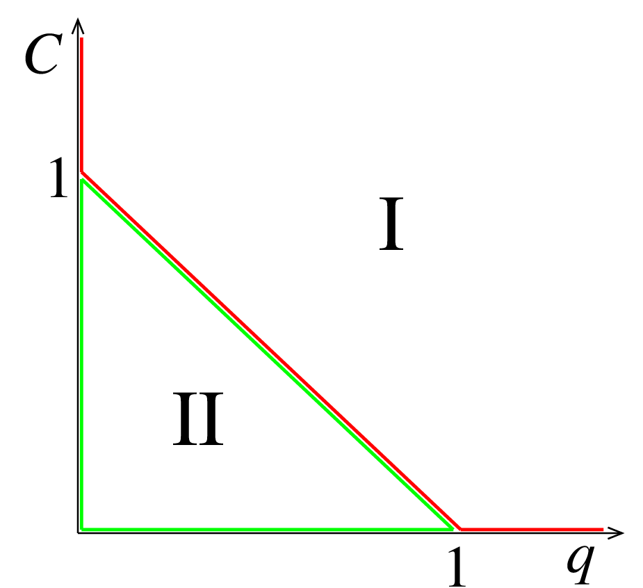
The model exhibits a continuous transition along the phase boundary between both phases (). The number of speakers of the unfavoured language vanishes linearly as the phase boundary is approached from the coexistence phase (see (5)), whereas the relaxation time diverges linearly as the phase boundary is approached from both sides (see (4) and (6)).
2.2 competing languages
The above setting can be extended to the case of an arbitrary number of competing languages in a given area. Languages, numbered , are more or less favoured, depending on their attractivenesses . The latter quantities are assumed to be quenched, i.e., fixed once for all. This non-trivial static profile of attractivenesses is responsible for conversions of single individuals from less attractive to more attractive languages.
Let be the total population of the area under consideration at time , and be the number of speakers of language number . The dynamics of the model are defined by the rate equations
| (8) | |||||
The terms underlined by braces describe the intrinsic dynamics of the numbers of speakers of each language. The novel feature here is again the presence of the parameter , which is responsible for imbalanced dynamics, allowing thus the possibility of language coexistence. The last term in (8) describes the conversions of single individuals. If language is more attractive than language , there is a net positive conversion rate from language to language . For the sake of simplicity, we assume that these conversion rates depend linearly on the differences of attractivenesses between departure and target languages, i.e.,
| (9) |
in some consistent units.
Throughout this work we shall not pay any attention to the evolution of the whole population . We therefore reformulate the model in terms of the fractions
| (10) |
of speakers of the various languages, which sum up to unity:
| (11) |
The reduction to be derived below is quite natural in the present setting. It provides an example of the reduction of Lotka-Volterra equations to replicator equations, proposed in [24] (see also [20, 21, 22]). In the present situation, for , which is precisely the range of where there is a possibility of language coexistence, the dynamics of the fractions obeys the following reduced rate equations, which can be derived from (8):
| (12) | |||||
with
| (13) |
and where attractivenesses and conversion rates have been rescaled according to
| (14) | |||||
| (15) |
In the following, we focus our attention onto the stationary states of the model, rather than on its dynamics. It is therefore legitimate to redefine time according to
| (16) |
so that equations (12) simplify to
| (17) |
The rate equations (17) for the fractions of speakers of the competing languages will be the starting point of further developments. The quantity can be alternatively viewed as a dynamical Lagrange multiplier ensuring that the dynamics conserves the sum rule (11). The above equations belong to the class of replicator equations (see e.g. [20, 21, 22]). Extensive studies of the dynamics of this class of equations have been made in mathematical biology, where the main focus has been on systematic classifications of fixed points and bifurcations in low-dimensional cases [24, 25, 26, 27, 28, 29].
From now on, we focus on the stationary state of the model for arbitrarily high values of the number of competing languages. The analysis of this goes as follows. The stationary values of the fractions of speakers are such that the right-hand sides of (17) vanish. For each language number , there are two possibilities: either , i.e., language gets extinct, or , i.e., language survives forever. The non-zero fractions of speakers of surviving languages obey the coupled linear equations
| (18) |
where the parameter is determined by expressing that the sum rule (11) holds in the stationary state. For generic values of model parameters, there is a unique stationary state, and the system relaxes exponentially fast to the latter, irrespective of its initial conditions. The uniqueness of the attractor is characteristic of the specific form of the rate equations (17), (18), with skew-symmetric conversion rates (see (15)). This has been demonstrated explicitly in the case of two competing languages, studied in detail in Section 2.1. The problem is however more subtle than it seems at first sight, as the number of surviving languages depends on model parameters in a non-trivial way.
2.3 The case of equally spaced attractivenesses
It is useful to consider first the simple case where the (reduced) attractivenesses of the competing languages are equally spaced between 0 and some maximal value that we denote by . Numbering languages in order of decreasing attractivenesses, so that language 1 is the most attractive and language the least attractive, this reads
| (19) |
We have
| (20) |
The parameter is therefore the mean attractiveness.
The (reduced) conversion rates read
| (21) |
so that the fixed-point equations (18) take the form
| (22) |
Already in this simple situation the number of surviving languages depends on the mean attractiveness in a non-trivial way.
Consider first the situation where all languages survive (). This is certainly true for , where there are no conversions, so that the solution is simply . There, all languages are indeed equally popular, as nothing distinguishes them. More generally, as long as all languages survive, the stationary solution obeying (22) reads
| (23) |
for . The above solution ceases to hold when the fraction of speakers of the least attractive language vanishes, i.e., . This first extinction takes place for the threshold value
| (24) |
of the mean attractiveness .
Consider now the general case where only among the languages survive. These are necessarily the most attractive ones, shown as red symbols in Figure 2.

In this situation, (22) yields
| (25) |
for . The linear relationship between the attractiveness of language and the stationary fraction of speakers of that language, observed in (23) and (25), is a general feature of the model (see Section 2.4). The fraction of speakers of the least attractive of the surviving languages vanishes at the following threshold mean attractiveness:
| (26) |
for .
The following picture therefore emerges for the stationary state of competing languages with equally spaced attractivenesses. The number of surviving languages decreases as a function of the mean attractiveness , from (all languages survive) near to (consensus) as very large . Less attractive languages become extinct one by one as every single one of the thresholds (26) is traversed, so that
| (27) |
Figure 3 illustrates this picture for 5 competing languages. In each of the sectors defined in (27), the stationary fractions of speakers of the surviving languages are given by (25). They depend continuously on the mean attractiveness , even though they are given by different expressions in different sectors. In particular, is flat, i.e., independent of , in the sector where . The fraction of speakers of the most attractive language grows monotonically as a function of , whereas all the other fractions of speakers eventually go to zero.

When the number of languages is large, the range of values of where the successive transitions take place is very broad. The threshold at which a consensus is reached, , is indeed much larger than the threshold at which the least attractive language disappears, . The ratio between these two extreme thresholds reads .
2.4 The general case
We now turn to the general case of competing languages with arbitrary reduced attractivenesses . Throughout the following, languages are numbered in order of decreasing attractivenesses, i.e.,
| (28) |
We shall be interested mostly in the stationary state of the model. As already mentioned above, the number of surviving languages depends on model parameters in a non-trivial way. The surviving languages are always the most attractive ones (see Figure 2). The fractions of speakers of those languages, obeying the fixed-point equations (18), can be written in full generality as
| (29) |
for , with
| (30) |
The existence of an explicit expression (29) for the solution of the fixed-point equations (18) in full generality is a consequence of their simple linear-minus-bilinear form, which also ensures the uniqueness of the attractor.
The number of surviving languages is the largest such that the solution (29) obeys for . Equivalently, is the largest integer in such that
| (31) |
Every single one of the differences involved in the sum is positive, so that:
| (32) |
From now on, we model attractivenesses as independent random variables. More precisely, we set
| (33) |
where is the mean attractiveness, and the rescaled attractivenesses are positive random variables drawn from some continuous distribution such that . For any given instance of the model, i.e., any draw of the random variables , languages are renumbered in order of decreasing attractivenesses (see (28)).
For concreteness we assume that is non-vanishing and that falls off more rapidly than at large . These hypotheses respectively imply that small values of are allowed with non-negligible probability and ensure the convergence of the second moment , where is the variance of .
Some quantities of interest can be expressed in closed form for all language numbers . One example is the consensus probability , defined as the probability of reaching consensus, i.e., of having (see (32)). This reads
| (34) |
We have
| (35) |
for all , where
| (36) |
is the cumulative distribution of .
In forthcoming numerical and analytical investigations we use the following distributions:
| (37) |
We begin our exploration of the model by looking at the dynamics of a typical instance of the model with languages and a uniform distribution of attractivenesses with . Figure 4 shows the time-dependent fractions of speakers of all languages, obtained by solving the rate equations (17) numerically, with the uniform initial condition for all . In this example there are surviving languages. The plotted quantities are observed to converge to their stationary values given by (29) for , and to zero for . They are ordered as the corresponding attractivenesses at all positive times, i.e., . Some of the fractions however exhibit a non-monotonic evolution. This is the case for in the present example.

Figure 5 shows the distribution of the number of surviving languages, for (top) and (bottom), and a uniform distribution of attractivenesses for four values of the product
| (38) |
This choice is motivated by the analysis of Appendix A. Each dataset is the outcome of draws of the attractiveness profile. The widths of the distributions are observed to shrink as is increased, in agreement with the expected behavior stemming from the law of large numbers. The corresponding mean fractions of surviving languages are shown in Table 1 to converge smoothly to the asymptotic prediction (A.35), i.e.,
| (39) |
with corrections.


| Eq. (39) | |||
|---|---|---|---|
| 2 | 0.750 | 0.718 | 0.70711 |
| 4 | 0.541 | 0.510 | 0.5 |
| 10 | 0.356 | 0.326 | 0.31623 |
| 30 | 0.222 | 0.192 | 0.18257 |
An overall picture of the dependence of the statistics of surviving languages on the mean attractiveness is provided by Figure 6, showing the mean number of surviving languages against , for and uniform and exponential attractiveness distributions. The plotted quantity decreases monotonically, starting from the value in the absence of conversions (), and converging to its asymptotic value in the limit, where consensus is reached with certainty. Its dependence on is observed to be steeper for the exponential distribution. These observations are corroborated by the asymptotic analysis of Appendix A. For the uniform distribution, (A.35) yields the scaling law . Concomitantly, the consensus probability becomes sizeable for (see (A.33)). For the exponential distribution, (A.38) yields the decay law , irrespective of , and the consensus probability is strictly independent of (see (A.36)).

3 Breaking spatial symmetry: language coexistence by inhomogeneous attractivenesses
As mentioned in the Introduction, different competing languages may coexist in distinct geographical areas, because they are more or less favoured locally, despite the homogenising effects of migration and language shift [9, 10, 11]. The aim of this section is to provide a quantitative understanding of this scenario. We continue to use the approach and the formalism of Section 2. We however take the liberty of adopting slightly different notations, as both sections are entirely independent.
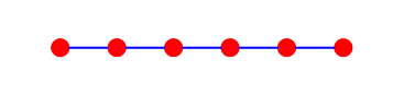
We consider the dynamics of two competing languages in a structured territory comprising several distinct geographic areas. For definiteness, we assume that the population of each area is homogeneous. We restrict ourselves to the geometry of an array of areas, where individuals can only migrate along the links joining neighbouring areas, as shown in Figure 7. We assume for simplicity that the migration rates between neighbouring areas are uniform, so that in the very long run single individuals eventually perform random walks across the territory. The relative attractivenesses of both competing languages are distributed inhomogeneously among the various areas, so that the net conversion rate from language 2 to language 1 depends on the area number . Finally, in order to emphasise the effects of spatial inhomogeneity on their own, we simplify the model by neglecting imbalance and thus set .
Let and denote the respective numbers of speakers of language 1 and of language 2 in area number at time . The dynamics of the model is defined by the coupled rate equations
| (40) | |||||
| (41) | |||||
The extremal sites and have only one neighbour. The corresponding equations have to be modified accordingly. The resulting boundary conditions can be advantageously recast as
| (42) |
and similarly for other quantities. These are known as Neumann boundary conditions.
The total populations of the various areas obey
| (43) | |||||
irrespective of the conversion rates . As a consequence, in the stationary state all areas have the same population, which reads in our reduced units. The corresponding stability matrix is given in (B.5). The population profile therefore converges exponentially fast to its uniform stationary value, with unit relaxation time ().
From now on we assume, for simplicity, that the total population of each area is unity in the initial state. This property is preserved by the dynamics, i.e., we have for all and , so that the rate equations (41) simplify to
| (44) | |||||
The rate equations (44) for the fractions of speakers of language 1 in the various areas provide another example of the broad class of replicator equations (see e.g. [20, 21, 22]). The above equations are the starting point of the subsequent analysis. In the situation where language 1 is uniformly favoured or disfavoured, so that the conversion rates are constant (), the above rate equations boil down to the discrete Fisher-Kolmogorov-Petrovsky-Piscounov (FKPP) equation [30, 31], which is known to exhibit traveling fronts, just as the well-known FKPP equation in the continuum [32, 33]. In the present context, the focus will however be on stationary solutions on finite arrays, obeying
| (45) |
3.1 Two geographic areas
We begin with the case of two geographic areas connected by a single link. The problem is simple enough to allow for an explicit exposition of its full solution. The rate equations (44) become
| (46) | |||
| (47) |
Because of the migration fluxes, for any non-zero it is impossible for any of the languages to become extinct in one area and survive in the other one. The only possibility is that of a uniform consensus, where one and the same language survives in all areas. The consensus state where language 1 survives is described by the stationary solution . The corresponding stability matrix is
| (48) |
where denotes a diagonal matrix (whose entries are listed), whereas is defined in (B.3). The stability condition amounts to
| (49) |
Similarly, the consensus state where language 2 survives is described by the stationary solution . The corresponding stability matrix is
| (50) |
The conditions for the latter to be stable read
| (51) |
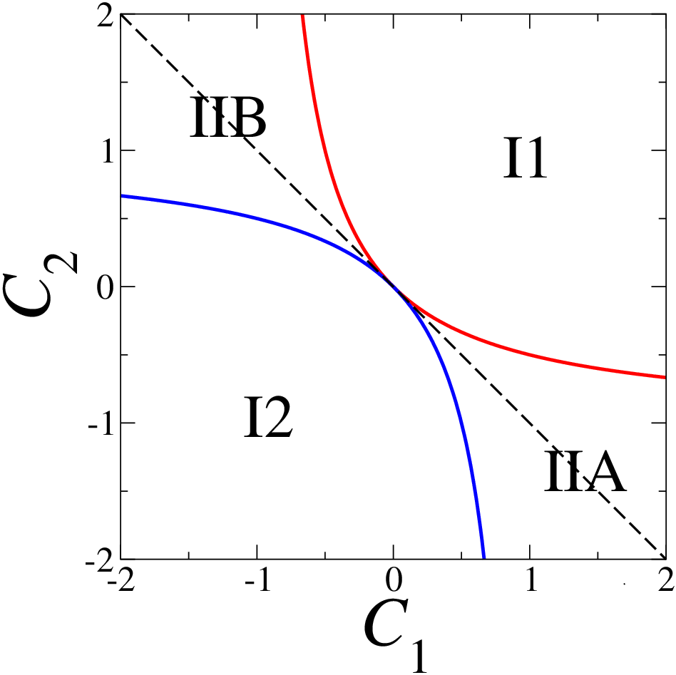
Figure 8 shows the phase diagram of the model in the – plane for . Region I1 is the consensus phase where language 1 survives. It is larger than the quadrant where this language is everywhere favoured (i.e., and are positive), as its boundary (red curve) reads . Similarly, region I2 is the consensus phase where language 2 survives. It is larger than the quadrant where this language is everywhere favoured (i.e., and are negative), as its boundary (blue curve) reads . The regions marked IIA and IIB are coexistence phases. These phases are located symmetrically around the line (black dashed line) where none of the languages is globally favoured. There, the fractions and of speakers of language 1 in both areas vary continuously between zero on the blue curve and unity on the red one, according to
| IIA: | (52) | ||||
| IIB: | (53) |
with
| (54) |
We have therefore
| (55) |
all over the coexistence phases IIA and IIB. The right-hand-side equals 0 on the blue curve, 1 on the black dashed line, and 2 on the red curve.
3.2 geographical areas
From now on we consider the general situation of geographic areas, as shown in Figure 7. The basic properties of the model can be inferred from the case of two areas, studied in section 3.1. In full generality, because of migration fluxes, it is impossible for any of the languages to become extinct in some areas and survive in some other ones. The only possibility is that of a uniform consensus, where one and the same language survives in all areas.
The consensus state where language 1 survives is described by the uniform stationary solution where for all . The corresponding stability matrix is
| (56) |
Similarly, the consensus state where language 2 survives corresponds to the stationary solution where for all . The corresponding stability matrix is
| (57) |
If all the conversion rates vanish, both the above matrices read , whose spectrum comprises one vanishing eigenvalue (see (B.4)). In the regime where all the conversion rates are small with respect to , perturbation theory tells us that the largest eigenvalues of and respectively read and , to leading order, where
| (58) |
We therefore predict that the average conversion rate determines the fate of the system in the regime where conversion rates are small with respect to . If language 1 is globally favoured, i.e., , the system reaches the consensus where language 1 survives, and vice versa.
In the generic situation where the conversion rates are comparable to , their dispersion around their spatial average broadens the spectra of the matrices and . As a consequence, the condition (resp. ) is necessary, albeit not sufficient, for the consensus where language 1 (resp. language 2) survives to be stable.
3.3 Ordered attractiveness profiles
This section is devoted to a simple situation where the attractiveness profiles of both languages are ordered spatially. More specifically, we consider the case where language 1 is favoured in the first (i.e., leftmost) areas, whereas language 2 is favoured in the last (i.e., rightmost) areas, with and . For the sake of simplicity, we choose to describe this situation by conversion rates that have unit magnitude, as shown in Figure 9:
| (59) |

The symmetric situation where is even and , so that , can be viewed as a generalisation of the case of two geographic areas, studied in Section 3.1, for , i.e., along the black dashed line of Figure 8. Both languages play symmetric roles, so that no language is globally preferred, and no consensus can be reached. As a consequence, both languages survive everywhere, albeit with non-trivial spatial profiles, which can be thought of as avatars of the FKPP traveling fronts mentioned above, rendered stationary by being pinned by boundary conditions. The upper panel of Figure 10 shows the stationary fraction of speakers of language 1 against area number, for (i.e., ) and several . The abscissa is chosen in order to have a symmetric plot. As one might expect, each language is preferred in the areas where it is favoured, i.e., we have for , whereas for . Profiles get smoother as the migration rate is increased. The width of the transition region is indeed expected to grow as
| (60) |
This scaling law is nothing but the large behaviour of the exact dispersion relation
| (61) |
(see (B.18)) between and the decay rate such that either or falls off as , with the natural identification .
The asymmetric situation where , so that , implying that language 1 is globally favoured, is entirely different. The system indeed reaches a consensus state where the favoured language survives, whenever the migration rate exceeds some threshold . This threshold, corresponding to the consensus state becoming marginally stable, only depends on the integers and . It is derived in Appendix B and given by the largest solution of (B.23).
This is illustrated in the lower panel of Figure 10, showing against for and , and the same values of as on the upper panel. The corresponding threshold reads . The whole profile shifts upwards while it broadens as is increased. It tends uniformly to unity as tends to , demonstrating the continuous nature of the transition where consensus is formed.


The threshold migration rate assumes a scaling form in the regime where and are large and comparable. Setting
| (62) |
so that the excess fraction identifies with the average conversion rate , the threshold rate grows quadratically with the system size , according to
| (63) |
where is the smallest positive solution of the implicit equation
| (64) |
which is a rescaled form of (B.23).
The quadratic growth law (63) is a consequence of the diffusive nature of migrations. The following limiting cases deserve special mention.
For , i.e., and relatively close to each other (), we have
| (65) |
yielding to leading order
| (66) |
For , i.e., , we have , up to exponentially small corrections, so that
| (67) |
The situation considered in the lower panel of Figure 10, i.e., , and , corresponds to , hence , so that
| (68) |
This scaling result predicts for , a good approximation to the exact value .
3.4 Random attractiveness profiles
We now consider the situation of randomly disordered attractiveness profiles. The conversion rates are modelled as independent random variables drawn from some symmetric distribution , such that and .
The first quantity we will focus on is the consensus probability . It is clear from a dimensional analysis of the rate equations (45) that depends on the ratio , the system size , and the distribution . Furthermore, is expected to increase with . It can be estimated as follows in the limiting situations where is either very small or very large.
In the regime where (e.g. far from the center in Figure 8), conversion effects dominate migration effects. There, a consensus where language 1 (resp. language 2) survives can only be reached if all conversion rates are positive (resp. negative). The total consensus probability thus scales as
| (69) |
Consensus is therefore highly improbable in this regime. In other words, coexistence of both languages is overwhelmingly the rule.
In the opposite regime where (e.g. in the vicinity of the center in Figure 8), migration effects dominate conversion effects. There, we have seen in Section 3.2 that the average conversion rate defined in (58) essentially determines the fate of the system. If language 1 is globally favoured, i.e., , then the system reaches the uniform consensus where language 1 survives, and vice versa. Coexistence is therefore rare in this regime, as it requires to be atypically small. The probability for this to occur, to be identified with , has been given a precise definition in Appendix B by means of the expansion (B.13) of as a power series in the , and estimated within a simplified Gaussian setting. In spite of the heuristic character of its derivation, the resulting estimate (B.17) demonstrates that the consensus probability scales as
| (70) |
all over the regime where the ratio and the system size are both large. Furthermore, taking (B.17) literally, we obtain the following heuristic prediction for the finite-size scaling function:
| (71) |
The scaling result (70) shows that the scale of the migration rate which is relevant to describe the consensus probability for a typical disordered profile of attractivenesses reads
| (72) |
This estimate grows less rapidly with than the corresponding threshold for ordered profiles, which obeys a quadratic growth law (see (63)). The exponent of the scaling law (72) can be put in perspective with the anomalous scaling of the localisation length in one-dimensional Anderson localisation near band edges. There is indeed a formal analogy between the stability matrices of the present problem and the Hamiltonian of a tight-binding electron in a disordered potential, with the random conversion rates replacing the disordered on-site energies. For the tight-binding problem, the localisation length is known to diverge as in the bulk of the spectrum, albeit only as in the vicinity of band edges [34, 35, 36, 37, 38]. Replacing by the system size and remembering that stands for , we recover (72). The exponent is therefore nothing but the inverse of the exponent of anomalous band-edge localisation.
Figure 11 shows a finite-size scaling plot of the consensus probability against . Data correspond to arrays of length with uniform and Gaussian distributions of conversion rates with . Each data point is the outcome of independent realisations. The thin black curve is a guide to the eye, suggesting that the finite-size scaling function is universal, i.e., independent of details of the conversion rate distribution. It has indeed been checked that the weak residual dependence of data points on the latter distribution becomes even smaller as is further increased. The full green curve shows the heuristic prediction (71), providing a semi-quantitative picture of the finite-size scaling function. For instance, consensus is reached with probability and respectively for and , according to actual data, whereas (71) respectively predicts and .

Besides the value of the consensus probability , the next question is what determines whether or not the system reaches consensus. In Section 3.2 it has been demonstrated that the average conversion rate defined in (58) essentially determines the fate of the system in the regime where migration effects dominate conversion effects. It has also been shown that the consensus denoted by I1, where language 1 survives, can only be stable for , whereas the consensus denoted by I2, where language 2 survives, can only be stable for . The above statements are made quantitative in Figure 12, showing the probability distribution of the average conversion rate , for a Gaussian distribution of conversion rates with . The total (i.e., unconditioned) distribution (black curves) is Gaussian. Red and blue curves show the distributions conditioned on consensus. They are indeed observed to live entirely on for I1 and on for I2. Finally, the distributions conditioned on coexistence (green curves, denoted by II) exhibit narrow symmetric shapes around the origin. Values of the migration rate are chosen so as to have three partial histograms with equal weights, i.e., a consensus probability . This fixes for (top) and for (bottom).


4 Discussion
An area of interest that is common to both physicists and linguists concerns the evolution of competing languages. It was long assumed that such competition would result in the dominance of one language above all its competitors, until some recent work hinted that coexistence might be possible under specific circumstances. We argue here that coexistence of two or more competing languages can result from two symmetry-breaking mechanisms – due respectively to imbalanced internal dynamics and spatial heterogeneity – and engage in a quantitative exploration of the circumstances which lead to this coexistence. In this work, both symmetry-breaking scenarios are dealt with on an equal footing.
In the first case of competing languages in a single geographical area, our introduction of an interpolation parameter , which measures the amount of imbalance in the internal dynamics, turns out to be crucial for the investigation of language coexistence. It is conceptually somewhat subtle, since it appears only in the saturation terms in the coupled logistic equations used here to describe language competition; in contrast to the conversion terms (describing language shift from a less to a more favoured language), its appearance is symmetric with respect to both languages. For multiply many competing languages, the ensuing rate equations for the fractions of speakers are seen to bear a strong resemblance to a broad range of models used in theoretical ecology, including Lotka-Volterra or predator-prey systems.
We first consider the case where the languages in competition in a single area have equally spaced attractivenesses. This simple situation allows for an exact characterisation of the stationary state. The range of attractivenesses is measured by the mean attractiveness . As this parameter is increased, the number of surviving languages decreases progressively, as the least favoured languages successively become extinct at threshold values of . Importantly, the range of values of between the start of the disappearances and the appearance of consensus grows proportionally to . There is therefore a substantial amount of coexistence between languages that are significantly attractive.
In the general situation, where the attractivenesses of the competing languages are modelled as random variables with an arbitrary distribution, the outcomes of numerical studies at finite are corroborated by a detailed asymptotic analysis in the regime of large . One of the key results is that the quantity (the product of the number of languages with the mean attractiveness ) determines many quantities of interest, including the mean fraction of surviving languages. The relation between and is however non-universal, as it depends on the full attractiveness distribution. This non-universality is most prominent in the regime where the mean attractiveness is large, so that only the few most favoured languages survive in the stationary state. The number of such survivors is found to obey a scaling law, whose non-universal critical exponent is dictated by the specific form of the attractiveness distribution near its upper edge.
As far as symmetry breaking via spatial heterogeneity is concerned, we consider the paradigmatic case of two competing languages in a linear array of geographic areas, whose neighbours are linked via a uniform migration rate . In the simplest situation of two areas, we determine the full phase diagram of the model as a function of as well as the conversion rates ruling language shift in each area. This allows us to associate different regions of phase space with either consensus or coexistence. Our analysis is then generalised to longer arrays of linked geographical regions. We first consider ordered attractiveness profiles, where language 1 is favoured in the leftmost areas, while language 2 is favoured in the rightmost ones. If the two blocks are of equal size so that no language is globally preferred, coexistence always results; however, the spatial profiles of the language speakers themselves are rather non-trivial. For blocks of unequal size, there is a transition from a situation of coexistence at low migration rates to a situation of uniform consensus at high migration rates, where the language favoured in the larger block is the only survivor in all areas. The critical migration rate at this transition grows as . We next investigate disordered attractiveness profiles, where conversion rates are modelled as random variables. There, the probability of observing a uniform consensus is given by a universal scaling function of , where is the width of the symmetric distribution of conversion rates.
The ratio between migration and conversion rates beyond which there is consensus – either with certainty or with a sizeable probability – grows with the number of geographic areas as for ordered profiles of attractivenesses, and as for disordered ones. The first exponent is a consequence of the diffusive nature of migrations, whereas the second one has been derived in Appendix B.2 and related to anomalous band-edge scaling in one-dimensional Anderson localisation. If geographical areas were arranged according to a more complex geometric structure, these exponents would respectively read and , with and being the fractal and spectral dimensions of the underlying structure (see [39, 40], and [41, 42] for reviews).
Finally, we remark on another striking formal analogy – that between the rate equations (17) presented here, and those of a spatially extended model of competitive dynamics [43], itself inspired by a model of interacting black holes [44]. In the latter, the non-trivial patterns of survivors on various networks and other geometrical structures were a particular focus of investigation, and led to the unearthing of universal behaviour. We believe that a network model of competing languages which combines both the symmetry-breaking scenarios discussed in this paper, so that every node corresponds to a geographical area with its own imbalanced internal dynamics, might lead to the discovery of similar universalities.
AM warmly thanks the Leverhulme Trust for the Visiting Professorship that funded this research, as well as the Faculty of Linguistics, Philology and Phonetics at the University of Oxford, for their hospitality.
Both authors contributed equally to the present work, were equally involved in the preparation of the manuscript, and have read and approved the final manuscript.
Appendix A Asymptotic analysis for a large number of competing languages in a single area
This Appendix is devoted to an analytical investigation of the statistics of surviving languages in a single geographic area, in the regime where the numbers of competing languages is large.
The properties of the attractiveness distribution of the languages are key to determining whether coexistence or consensus will prevail. In particular the transition to consensus depends critically, and non-universally, on the way in which the attractiveness distribution decays, as will be shown below.
Statistical fluctuations between various instances of the model become negligible for large , so that sharp (i.e., self-averaging) expressions can be obtained for many quantities of interest.
Let us begin with the simplest situation where all languages survive. When the number of competing languages is large, the condition for this to occur assumes a simple form. Consider the expression (29) for . The law of large numbers ensures that the sum converges to
| (A.1) |
whereas is relatively negligible. The condition that all the competing languages survive therefore takes the form of a sharp inequality at large , i.e.,
| (A.2) |
All over this regime, the expression for simplifies to
| (A.3) |
The above analysis can be extended to the general situation where the numbers of competing languages and of surviving ones are large and comparable, with the fraction of surviving languages,
| (A.4) |
taking any value in the range .
The rescaled attractiveness of the least favoured surviving language, namely
| (A.5) |
turns out to play a key role in the subsequent analysis. Let us introduce for further reference the truncated moments ()
| (A.6) |
First of all, the relationship between and becomes sharp in the large- regime. We have indeed
| (A.7) |
The limits of all quantities of interest can be similarly expressed in terms of . We have for instance
| (A.8) |
for the sum introduced in (30). The marginal stability condition, namely that language number is at the verge of becoming extinct, translates to
| (A.9) |
The asymptotic dependence of the fraction of surviving languages on the rescaled mean attractiveness is therefore given in parametric form by (A.7) and (A.9). The identity
| (A.10) |
demonstrates that is a decreasing function of , as it should be.
When the parameter reaches unity from above, the model exhibits a continuous transition from the situation where all languages survive. The parameter vanishes linearly as
| (A.11) |
with unit prefactor, irrespective of the attractiveness distribution. The fraction of surviving languages departs linearly from unity, according to
| (A.12) |
In the regime where , the fraction of surviving languages is expected to fall off to zero. As a consequence of (A.7), corresponds to the parameter being close to the upper edge of the attractiveness distribution . This is to be expected, as the last surviving languages are the most attractive ones. As a consequence, the form of the relationship between and for is highly non-universal, as it depends on the behavior of the distribution near its upper edge. It turns out that the following two main classes of attractiveness distributions have to be considered.
- •
Class 1: Power law at finite distance.
Consider the situation where the distribution has a finite upper edge , and either vanishes or diverges as a power law near this edge, i.e.,
(A.13) The exponent is positive. The density diverges near its upper edge for , whereas it vanishes near for , and takes a constant value for .
In the relevant regime where is close to , the expressions (A.7) and (A.9) simplify to
(A.14) (A.15) Eliminating between both above estimates, we obtain the following power-law relationship between and :
(A.16) In terms of the original quantities and , the above result reads
(A.17) Setting in this estimate, we predict that the consensus probability becomes appreciable when
(A.18) - •
Class 2: Power law at infinity.
Consider now the situation where the distribution extends up to infinity, and falls off as a power law, i.e.,
(A.19) The exponent is larger than 2, in order for the first two moments of to be convergent.
In the relevant regime where is large, the expressions (A.7) and (A.9) simplify to
(A.20) (A.21) Eliminating between both above estimates, we obtain the following power-law relationship between and :
(A.22) In terms of the original quantities and , the above result reads
(A.23) Setting in this estimate, we predict that the consensus probability becomes appreciable when
(A.24)
We now summarise the above discussion. In the regime where , the fraction of surviving languages falls off as a power law of the form
| (A.25) |
where the positive exponent varies continuously, according to whether the distribution of attractivenesses extends up to a finite distance or infinity (see (A.16), (A.22)):
| (A.26) |
In the marginal situation between both classes mentioned above, comprising e.g. the exponential distribution, the decay exponent sticks to its borderline value
| (A.27) |
The decay law might however be affected by logarithmic corrections.
Another view of the above scaling laws goes as follows. When the number of languages is large, the number of surviving languages decreases from to over a very broad range of mean attractivenesses. The condition for all languages to survive (see (A.2)) sets the beginning of this range as
| (A.28) |
The occurrence of a sizeable consensus probability sets the end of this range as
| (A.29) |
where the exponent varies continuously, according to (see (A.18), (A.24)):
| (A.30) |
In the marginal situation between both classes, the above exponent sticks to its borderline value
| (A.31) |
The extension of the dynamical range, defined as the ratio between both scales defined above, diverges as
| (A.32) |
We predict in particular a linear divergence for the exponential distribution () and a quadratic divergence for the uniform distribution (). This explains the qualitative difference observed in Figure 6. The slowest growth of the dynamical range is the square-root law observed for distributions falling off as a power-law with , so that .
To close, let us underline that most of the quantities met above assume simple forms for the uniform and exponential distributions (see (37)).
- •
Uniform distribution.
- •
Exponential distribution.
Appendix B Stability matrices and their spectra
B.1 Generalities
This Appendix is devoted to stability matrices and their spectra. Let us begin by reviewing some general background (see e.g. [45] for a comprehensive overview). Consider an autonomous dynamical system defined by a vector field in dimensions, i.e., by coupled first-order equations of the form
| (B.1) |
with , where the right-hand sides depend on the dynamical variables themselves, but not explicitly on time.
Assume the above dynamical system has a fixed point , such that for all . Small deviations around the fixed point obey the linearised dynamics given by the stability matrix , i.e., the matrix defined by
| (B.2) |
where right-hand sides are evaluated at the fixed point. The fixed point is stable, in the strong sense that small deviations fall off exponentially fast to zero, if all eigenvalues of have negative real parts. In this case, if all the are real, their opposites are the inverse relaxation times of the linearised dynamics. In particular, the opposite of the smallest eigenvalue, simply denoted by , characterises exponential convergence to the fixed point for a generic initial state. If some of the have non-zero imaginary parts, convergence is oscillatory.
B.2 Array models
The remainder of this Appendix is devoted to the stability matrices involved in the array models considered in Section 3, for an arbitrarily large number of geographical areas. All those stability matrices are related to the symmetric matrix
| (B.3) |
representing (minus) the Laplacian operator on a linear array of sites, with Neumann boundary conditions. References [46, 47] provide reviews on the Laplacian and related operators on graphs.
The eigenvalues of and the corresponding normalised eigenvectors , such that and , read
| (B.4) |
(). The vanishing eigenvalue corresponds to the uniform eigenvector .
Let us begin by briefly considering the simple example of the stability matrix
| (B.5) |
of the rate equations (43) for the total populations . Its eigenvalues are . The smallest of them is , so that the inverse relaxation time is given by , as announced below (43).
Let us now consider the stability matrices
| (B.6) |
respectively defined in (56) and (57), and corresponding to both uniform consensus states for an arbitrary profile of conversion rates . The ensuing stability conditions have been written down explicitly in (49) and (51) for . It will soon become clear that it is virtually impossible to write them down for an arbitrary size . Some information can however be gained from the calculation of the determinants of the above matrices. They only differ by a global sign change of all the conversion rates , so that it is sufficient to consider . It is a simple matter to realise that its determinant reads
| (B.7) |
where is a generalised eigenvector solving the following Cauchy problem:
| (B.8) |
with initial conditions . We thus obtain recursively
| (B.9) | |||||
| (B.10) | |||||
| (B.11) | |||||
and so on. The expression (B.10) for agrees with the second of the conditions (49) and with the equation of the red curve in Figure 8, as should be. The expression (B.11) for demonstrates that the complexity of the stability conditions grows rapidly with the system size .
Random arrays
In the case of random arrays, considered in Section 3.4, the conversion rates are independent random variables such that and .
The regime of most interest is where the conversion rates are small with respect to . In this regime, the determinant can be expanded as a power series in the conversion rates. The solving the Cauchy problem (B.8) are close to unity. Setting
| (B.12) |
where the are linear and the quadratic in the , we obtain after some algebra
| (B.13) |
where
| (B.14) |
are respectively linear and quadratic in the . We have
| (B.15) |
In Section 3.4 we need an estimate of the probability that is atypically small. Within the present setting, it is natural to define the latter event as . The corresponding probability can be worked out proviso we make the ad hoc simplifying assumptions – that definitely do not hold in the real world – that and are Gaussian and independent. Within this framework, the complex Gaussian random variable
| (B.16) |
has an isotropic density in the complex plane. We thus obtain
| (B.17) |
Ordered arrays
The aim of this last section is to investigate the spectrum of the stability matrix associated with the ordered profile of conversion rates given by (59).
In this case, the generalised eigenvector solving the Cauchy problem (B.8) can be worked out explicitly. We have for , and therefore , where obeys the dispersion relation
| (B.18) |
The initial conditions fix and , and so
| (B.19) |
Similarly, we have for , with , and therefore , where obeys the dispersion relation
| (B.20) |
Matching both solutions for and fixes and , and so
| (B.21) | |||||
Inserting the latter result into (B.7), we obtain the following expression for the determinant of , with :
| (B.22) | |||||
The vanishing of the above expression, i.e.,
| (B.23) |
signals that one eigenvalue of the stability matrix vanishes. In particular, the consensus state where language 1 survives becomes marginally stable at the threshold migration rate , where the largest eigenvalue of vanishes. Equation (B.23) amounts to a polynomial equation of the form , where the polynomial has degree . All its zeros are real, and is the largest of them. The first of these polynomials read
| (B.24) |
References
- [1] C. Castellano, S. Fortunato, V. Loreto, Rev. Mod. Phys. 81, 591 (2009)
- [2] R.A. Blythe, Eur. Phys. J. B 88, 295 (2015)
- [3] M. Krauss, Language 68, 41 (1992)
- [4] D. Crystal, Language Death (Cambridge University Press, Cambridge, 2000)
- [5] W.J. Sutherland, Nature 423, 276 (2003)
- [6] D.M. Abrams, S.H. Strogatz, Nature 424, 900 (2003)
- [7] D. Stauffer, X. Castello, V.M. Eguiluz, M.S. Miguel, Physica A 374, 835 (2007)
- [8] M. Zhang, T. Gong, Proc. Nat. Acad. Sci. USA 110, 9698 (2013)
- [9] M. Patriarca, T. Leppanen, Physica A 338, 296 (2004)
- [10] X. Castello, V.M. Eguiluz, M.S. Miguel, New J. Phys. 8, 308 (2006)
- [11] R. Fujie, K. Aihara, N. Masuda, J. Stat. Phys. 151, 289 (2013)
- [12] J.P. Pinasco, L. Romanelli, Physica A 361, 355 (2006)
- [13] A. Kandler, J. Steele, Biol. Theory 3, 164 (2008)
- [14] A. Kandler, R. Unger, J. Steele, Phil. Trans. R. Soc. B 365, 3855 (2010)
- [15] J. Mira, A. Paredes, Europhys. Lett. 69, 1031 (2005)
- [16] J.W. Minett, W.S.Y. Wang, Lingua 118, 19 (2008)
- [17] R. Colucci, J. Mira, J.J. Nieto, M.V. Otero-Espinar, Acta Appl. Math. 146, 187 (2016)
- [18] N.L. Komarova, P. Niyogi, M.A. Nowak, J. Theor. Biol. 209, 43 (2001)
- [19] A.A. Berryman, Ecology 73, 1530 (1992)
- [20] J. Hofbauer, K. Sigmund, Evolutionary Games and Population Dynamics (Cambridge University Press, Cambridge, 1998)
- [21] J. Hofbauer, K. Sigmund, Bull. Amer. Math. Soc. 40, 479 (2003)
- [22] M.A. Nowak, K. Sigmund, Science 303, 793 (2004)
- [23] A.J. Lotka, Elements of Physical Biology (Williams & Wilkins, Baltimore, 1925)
- [24] J. Hofbauer, Nonlinear Anal. 5, 1003 (1981)
- [25] P.D. Taylor, L.B. Jonker, Math. Biosci. 40, 145 (1978)
- [26] I.M. Bomze, Biol. Cybern. 48, 201 (1983)
- [27] P.F. Stadler, P. Schuster, Bull. Math. Biol. 52, 485 (1990)
- [28] I.M. Bomze, Biol. Cybern. 72, 447 (1995)
- [29] P.F. Stadler, P. Schuster, Bull. Math. Biol. 57, 21 (1995)
- [30] B. Zinner, G. Harris, W. Hudson, J. Diff. Eq. 105, 46 (1993)
- [31] M. Barthélemy, C. Godrèche, J.M. Luck, J. Theor. Biol. 267, 554 (2010)
- [32] R.A. Fisher, Ann. Eugenics 7, 353 (1937)
- [33] A. Kolmogorov, I. Petrovsky, N. Piscounov, Moscow Univ. Bull. Math. 1, 1 (1937)
- [34] H.L. Frisch, S.P. Lloyd, Phys. Rev. 120, 1175 (1960)
- [35] B.I. Halperin, Phys. Rev. 139, A104 (1965)
- [36] B. Derrida, E.J. Gardner, J. Phys. (France) 45, 1283 (1984)
- [37] F.M. Izrailev, S. Ruffo, L. Tessieri, J. Phys. A 31, 5263 (1998)
- [38] A. Comtet, J.M. Luck, C. Texier, Y. Tourigny, J. Stat. Phys. 150, 13 (2013)
- [39] S. Alexander, R. Orbach, J. Phys. (France) Lett. 43, L625 (1982)
- [40] R. Rammal, G. Toulouse, J. Phys. (France) Lett. 44, L13 (1983)
- [41] S. Havlin, D. Ben-Avraham, Adv. Phys. 36, 695 (1987)
- [42] J.W. Haus, K.W. Kehr, Phys. Rep. 150, 263 (1987)
- [43] J.M. Luck, A. Mehta, Phys. Rev. E 92, 052810 (2015)
- [44] J.M. Luck, A. Mehta, Eur. Phys. J. B 44, 79 (2005)
- [45] A. Katok, B. Hasselblatt, Introduction to the Modern Theory of Dynamical Systems (Cambridge University Press, Cambridge, 1995)
- [46] R.J. Wilson, Introduction to Graph Theory (Longman, London, 1979)
- [47] B. Bollobas, Modern Graph Theory (Springer, New York, 1998)