Computing the Pseudospectral Abscissa of Time-Delay Systems

The pseudospectra provide information about the characteristic roots of the system when the system matrices in the characteristic equation are subject to perturbations. They are closely related with the robust stability of the system and distance to instability, Trefethen 1997. We consider the characteristic equation of the time-delay systems:

where

$A_{i}\in\mathbb{C}^{n\times n}$, $\tau_{i}\in\mathbb{R}_{0}^{+}$ for $i=0,\ldots,m$ and $\tau_{0}=0$. The maximum real part of the characteristic roots is the spectral abscissa,

When the system matrices in (2) is subject to the perturbations, the pseudospectra of the characteristic equation (1) is defined as

where perturbations on the systems matrices are represented as

$\delta A_{i}\in\mathbb{C}^{n\times n}$ and satisfying $\|\delta A_{i}\|_{2}\leq\frac{\epsilon}{w_{i}}$ for $i=0,\ldots,m$. Here the $w_{i}\in\mathbb{R}_{0}^{+}$ $i=0,\ldots,m$ are some weights on the perturbations which can be chosen apriori. The maximum real part in the pseudospectra is the pseudospectral abscissa which is defined as

The computation of the pseudospectral abscissa for finite dimensional systems corresponds to the special case of (1):

In this particular case, the pseudospectra can be equivalently expressed as Boyd et al. 1989

where $\sigma_{\max}(A)$ is the largest singular value of the matrix $A$. Note that this definition reduces the pseudospectra boundary to the level set of the resolvent norm. This connection is used to compute the distance to instability and pseudospectral abscissa via a bisection algorithm in Byers 1988 and Burke et al. 2003a respectively. A quadratically convergent algorithm for the pseudospectral abscissa computation is given in Burke et al. 2003b based on a ‘criss-cross’ procedure. In Michiels et al. 2006, these results are extended to matrix functions of the form (2) where the perturbations take the form of (5). In particular, it is shown in Theorem $1$ that the pseudospectral abscissa as defined in (4) can be expressed in the following way:

where

Using the pseudospectra definition in (8), the pseudospectral abscissa in (6) can be rewritten as

The supremum in the definition (10) is well-defined since $F^{-1}(\lambda)$ is a strictly proper function and $w(\lambda)$ is uniformly bounded on any right half complex plane in (9).

In Section 2, a bisection algorithm is given for pseudospectral abscissa computation of time-delay systems based on the connection between the pseudospectra and the level sets of the function $f(\lambda)$.

This algorithm is implemented in two steps: first the approximate pseudospectral abscissa is computed by the prediction step in Section 3 and then the approximate results are corrected in Section 4.

The overall algorithm for the pseudospectral abscissa computation is outlined in Section 5. A numerical example and concluding remarks can be found in Sections 6 and 7.

Notation:
The notation in the paper is standard and given below. $\mathbb{C},\mathbb{R}:$ the field of the complex and real numbers, $\mathbb{R}_{0}^{+}:$ the positive real numbers including zero, $\Re(u):$ real part of the complex number $u$, $\Im(u):$ imaginary part of the complex number $u$. $|u|:$ magnitude of the complex number $u$. $\bar{u}:$ conjugate of the complex number $u$. $A^{*}:$ complex conjugate transpose of the matrix $A$. $I_{n\times n}:$ identity matrix with dimension $n$. $\sigma_{\max}(A):$ the largest singular value of the matrix $A$. $\|F(j\omega)\|_{\infty}:$ $\mathcal{L}_{\infty}$ norm of the transfer function $F$

Given the function $f$ in (9), define the function $\alpha_{f}(\sigma)$ as:

over $\sigma\in(\alpha_{0},\infty)$.

Similarly, it can be shown that the case $\alpha_{f}(\sigma_{1})=\alpha_{f}(\sigma_{2})$ with $\sigma_{0}<\sigma_{1}<\sigma_{2}$ is a contradiction with the continuity of the individual eigenvalues. $\Box$

Using the definition in (10), the pseudospectral abscissa is the $\sigma$ value of the function where $\alpha_{f}(\sigma)=\frac{1}{\epsilon}$. Since the function $\alpha_{f}(\sigma)$ is strictly decreasing by Proposition 1 and it attains all the values from $0$ to $\infty$ by Proposition 2, the pseudospectral abscissa can be calculated by the following bisection algorithm.

The main computation in the bisection algorithm is to check whether the inequality in step $2.3$ is satisfied. By algebraic computation, the function $\alpha_{f}(\sigma)$ is equivalent to

where

and

The inequality $\alpha_{f}(\sigma)>\frac{1}{\epsilon}$ in step $2.3$ is satisfied if and only if $F_{\sigma}^{-1}(j\omega)$ has a singular value equal to $\frac{1}{\epsilon w(\sigma)}$ for some value of $\omega$. This condition can be reduced into the verification of the imaginary axis eigenvalues of an infinite dimensional operator as shown in the following Theorem.

Using Theorem 3, we can refine the conceptual algorithm for the pseudospectral abscissa computation,

Note that step $2.3$ in the Algorithm 3 requires solving a linear infinite dimensional eigenvalue problem for $\mathcal{L}_{\sigma}$ which needs to be discretized in a practical implementation. We will do this using a spectral method (see, e.g. Trefethen 2000; Breda et al. 2005; Breda et al. 2006) and calculate the approximate solution by solving the standard linear eigenvalue problem. This approach is described in the next section.

Given a positive integer $N$, we consider a mesh $\Omega_{N}$ of $2N+1$ distinct points in the interval $[-\tau_{\max},\ \tau_{\max}]$:

where

This allows to replace the continuous space $X$ with the space $X_{N}$ of discrete functions defined over the mesh $\Omega_{N}$, i.e. any function $\phi\in X$ is discretized into a block vector $x=[x_{-N}^{T}\cdots\ x_{N}^{T}]^{T}\in X_{N}$ with components

Let $\mathcal{P}_{N}x,\ x\in X_{N}$ be the unique $\mathbb{C}^{2n}$ valued interpolating polynomial of degree $\leq 2N$ satisfying

In this way, the operator $\mathcal{L}_{\sigma}$ over $X$ can be approximated with the matrix $\mathcal{L}_{\sigma}^{N}:\ X_{N}\rightarrow X_{N}$, defined as

Using the Lagrange representation of $\mathcal{P}_{N}x$,

where the Lagrange polynomials $l_{N,k}$ are real valued polynomials of degree $2N$ satisfying

we obtain the explicit form

where

Note that all the problem specific information and the parameter $\sigma$ are concentrated in the middle row of $\mathcal{L}_{\sigma}^{N}$, i.e. the elements $(a_{-N},\ldots,a_{N})$, while all other elements of $\mathcal{L}_{\sigma}^{N}$ can be computed beforehand.

Since step $2.3$ of Algorithm 2 is based on checking the presence of eigenvalues of $\mathcal{L}_{\sigma}$ on the imaginary axis and thus strongly rely on the symmetry of the eigenvalues with respect to the imaginary axis, it is important that this property is preserved in the discretization. The following Proposition gives the condition on the mesh such that this symmetry holds.

Based on the discretization of $\mathcal{L}_{\sigma}$ into $\mathcal{L}_{\sigma}^{N}$, we propose the following algorithm to approximate (predict) the pseudospectral abscissa. It corresponds to Algorithm 2 where step $2.3$ is replaced with the matrix $\mathcal{L}_{\sigma}^{N}$ for a fixed $N$.

In what follows we clarify the effect of using the discretized operator in the algorithm. The next Theorem establishes the link between the imaginary axis eigenvalues of $\mathcal{L}_{\sigma}^{N}$ and the corresponding inequality check condition similar to the connection between $\mathcal{L}_{\sigma}$ and the inequality (15) in Theorem 3.

Therefore, the effect of using $\mathcal{L}_{\sigma}^{N}$ instead of $\mathcal{L}_{\sigma}$ corresponds to computing the approximate pseudospectral abscissa

The accuracy of the approximation depends on the discretization parameter $N$. Therefore, the accuracy can be chosen arbitrarily close to $\alpha_{\epsilon}$ by increasing $N$. Note that at each iteration of step $2.3$ in Algorithm 3, an eigenvalue problem of size $(2n)(2N+1)$ needs to be solved which may be computationally very demanding for large $N$.

However, because the eigenvalues of $\mathcal{L}_{\sigma}^{N}$ exhibit the spectral convergence to the corresponding eigenvalues of $\mathcal{L}_{\sigma}$ (following the lines of Breda et al. 2005) and because the approximation error can be corrected in a very cheap way as we shall see in the next section, it is sufficient to have a small value of $N$ for most practical applications.

The Bisection Algorithm 3 finds the complex points $\tilde{\lambda}_{i}=\tilde{\sigma}+j\tilde{\omega}_{i}$ for $i=1,\ldots,\tilde{n}$ achieving the approximate pseudospectral abscissa $\tilde{\sigma}$ which is close to the $\alpha_{\epsilon}$ given tolerance and discretization points $N$. These approximate results are corrected by using the property that the eigenvalues of the pseudospectral abscissa appear as solutions of a finite dimensional nonlinear eigenvalue problem. The following theorem establishes the link between this nonlinear eigenvalue problem and the linear eigenvalue problem of $\mathcal{L}_{\sigma}$.

The solutions of (24) can be found by solving

which in general has an infinite number of solution.

The correction method is based on the property that if $\omega(\sigma)\|F_{\sigma}^{-1}(j\omega)\|_{\infty}=\frac{1}{\epsilon}$, then the operator $\mathcal{L}_{\sigma}$, or equivalently, (26) has a multiple non-semisimple eigenvalue as shown in Figure 2:

If $\lambda_{\epsilon}=\alpha_{\epsilon}+j\omega_{\epsilon}$ are such that

then setting

the pair $(\omega,\alpha)=(\omega_{\epsilon},\alpha_{\epsilon})$ satisfies

These complex-valued equations seem over-determined but this is not the case due to the spectral properties of $H_{\sigma}(\lambda)$. Using the symmetry of the eigenvalues of the nonlinear eigenvalue problem (26) with respect to imaginary axis, we can write the following:

In conclusion, as a result of the bisection algorithm in the prediction step, the approximate pseudospectral abscissa $\tilde{\sigma}$ and the corresponding critical frequencies $\tilde{\omega}_{i}$ for $i=1,\ldots,\tilde{n}$ are calculated. Note that these computations are based on the approximation of $\mathcal{L}_{\sigma}$ into a matrix $\mathcal{L}_{\sigma}^{N}$. Using these approximate results as estimates of $(\omega_{\epsilon},\alpha_{\epsilon})$ (27), we can compute the approximate eigenvectors $u$ and $v$. These approximate values improved in the correction step by solving (34). At the end of the correction step, the pseudospectral abscissa $\sigma=\alpha_{\epsilon}$ and the achieved frequency $\omega=\omega_{\epsilon}$ are obtained within predefined tolerance.

The overall algorithm for computing the pseudospectral abscissa consists of two steps: the prediction step and the correction step. The first step requires a repeated computation of the eigenvalues of a $(2N+1)2n\times(2N+1)2n$ matrix $\mathcal{L}_{\sigma}^{N}$. The second step solves (34) with $4n+3$ equations and $4n+2$ unknowns using Gauss-Newton algorithm. Our method chooses $N$ sufficiently large such that the results of the prediction step are good starting values for the correction step. Note that by increasing $N$ and using only the prediction step, the approximate pseudospectral abscissa can be computed arbitrarily close to $\alpha_{\epsilon}$. However, this approach has more numerical cost than the combined approach when $N$ is large.

In our implementation, mesh points are chosen as Chebyshev extremal points since the corresponding interpolation polynomial has less oscillation towards the end of the interval compared to another distribution of mesh points, Breda et al. 2006.

Note that the spectral abscissa calculation in the prediction step requires the calculation of the right-most eigenvalue of time-delay systems. This computation is done by DDE-BIFTOOL, Engelborghs et al. 2002. The overall algorithm is fully automated and implemented as a MATLAB function.

We tested the numerical method on several benchmark problems. We generated the following difficult example to benchmark our method. We consider a time-delay system $F$ in (2) with the dimensions $m=7$, $n=10$, $n_{u}=2$, $n_{y}=4$ with delays $\tau_{1}=0.1$, $\tau_{2}=0.2$, $\tau_{3}=0.3$, $\tau_{4}=0.4$, $\tau_{5}=0.5$, $\tau_{6}=0.6$, $\tau_{7}=0.8$. The weights $w_{i}$ are set to $1$ and $\epsilon=0.1$. The pseudospectra is shown with black lines and black stars indicate the characteristic roots of (1) in Figure 3.

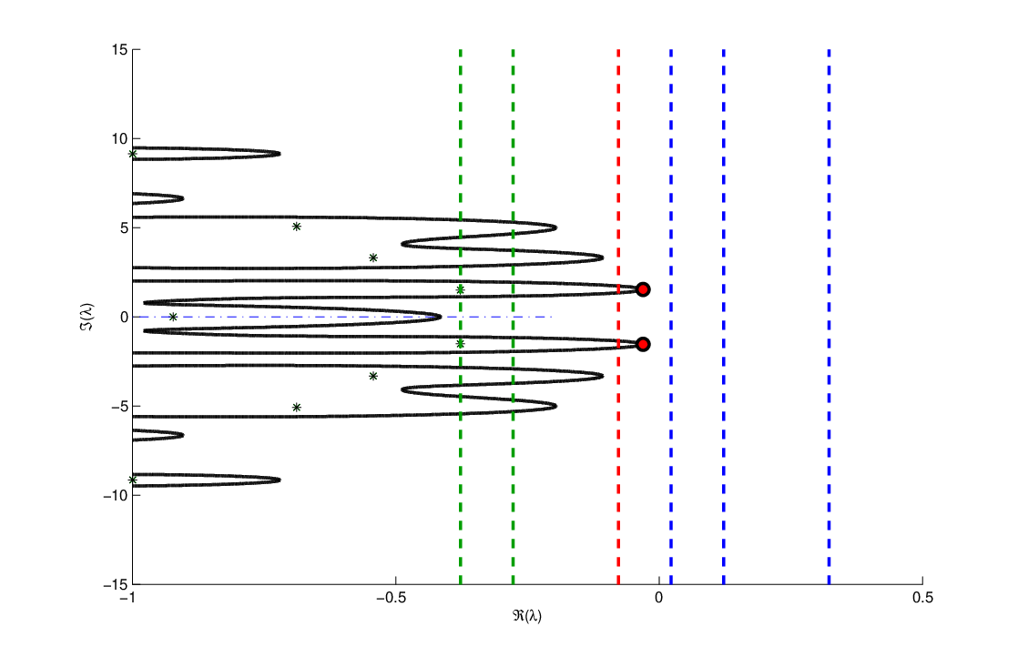
The tolerance in the bisection algorithm is set to $0.05$ and the discretization parameter is chosen as $N=6$. Each iteration of the while loop in the prediction step computes $\sigma_{M}$ and updates $\sigma_{L}$ or $\sigma_{R}$ shown as the vertical green and blue lines respectively. The approximate pseudospectral abscissa as a result of the prediction step is $\tilde{\sigma}=-0.0774$ and the corresponding critical frequencies are $\tilde{\omega}_{1}=1.3493$, $\tilde{\omega}_{2}=1.7318$.

These approximate values are improved in the correction step and the computed pseudospectral abscissa is $\alpha_{\epsilon}=-0.0307$ at $\omega_{\epsilon}=1.5383$ shown as red dots in Figure 3.

An accurate method to compute the pseudospectral abscissa of retarded time-delay systems with arbitrary number of delays is given. The method is based on two steps: The prediction step calculates the approximate pseudospectral abscissa using the connection between pseudospectra and the level set of a function. The correction step computes the pseudospectral abscissa by solving equations based on the nonlinear eigenvalue problem. The method is successfully applied to the moderate size example and its effectiveness is shown.

This article present results of the Belgian Programme on Interuniversity Poles of Attraction, initiated by the Belgian State, Prime Minister’s Office for Science, Technology and Culture, and of OPTEC, the Optimization in Engineering Centre of the K.U.Leuven.

References

- Boyd et al. (1989) Boyd, S., Balakrishnan, V., and Kabamba, P. (1989). A bisection method for computing the -norm of a transfer matrix and related problems. Mathematics of Control, Signals, and Systems, 2, 207–219.
- Breda et al. (2005) Breda, D., Maset, S., and Vermiglio, R. (2005). Pseudospectral differencing methods for characteristic roots of delay differential equations. SIAM Journal on Scientific Computing, 27, 482–495.
- Breda et al. (2006) Breda, D., Maset, S., and Vermiglio, R. (2006). Pseudospectral approximation of eigenvalues of derivative operators with non-local boundary conditions. Applied Numerical Mathematics, 56, 318–331.
- Burke et al. (2003a) Burke, J., Lewis, A., and Overton, M. (2003a). Optimization and pseudospectra, with applications to robust stability. SIAM Journal on Matrix Analysis and Applications, 25, 80–104.
- Burke et al. (2003b) Burke, J., Lewis, A., and Overton, M. (2003b). Robust stability and a criss-cross algorithm for pseudospectra. IMA Journal of Numerical Analysis, 23, 359–375.
- Byers (1988) Byers, R. (1988). A bisection method for measuring the distance of a stable matrix to the unstable matrices. SIAM Journal on Scientific and Statistical Computing, 9, 875–881.
- Engelborghs et al. (2002) Engelborghs, K., Luzyanina, T., and Roose, D. (2002). Numerical bifurcation analysis of delay differential equations using dde-biftool. ACM Transactions on Mathematical Software, 28, 1–21.
- Genin et al. (2002) Genin, Y., Stefan, R., and Dooren, P.V. (2002). Real and complex stability radii of polynomial matrices. Linear Algebra and its Applications, 351-352, 381–410.
- Gumussoy and Michiels (2009) Gumussoy, S. and Michiels, W. (2009). Computing norms of time-delay systems. submitted to IEEE Conference on Decision and Control.
- Hryniv and Lancaster (1999) Hryniv, R. and Lancaster, P. (1999). On the perturbation of analytic matrix functions. Integral Equations and Operator Theory, 34, 325–338.
- Michiels et al. (2006) Michiels, W., Green, K., Wagenknecht, T., and Niculescu, S.I. (2006). Pseudospectra and stability radii for analytic matrix functions with application to time-delay systems. Linear Algebra and its Applications, 418, 315–335.
- Trefethen (1997) Trefethen, L. (1997). Pseudospectra of linear operators. SIAM Review, 39, 383–406.
- Trefethen (2000) Trefethen, L. (2000). Spectral methods in MATLAB. volume 10 of Software, Environments, and Tools, SIAM.