Wide-bandwidth atomic magnetometry via instantaneous-phase retrieval
Abstract
We develop and demonstrate a new protocol that allows sensing of magnetic fields in an extra-ordinary regime for atomic magnetometry. Until now, the demonstrated bandwidth for atomic magnetometry has been constrained to be slower than the natural precession of atomic spins in a magnetic field—the Larmor frequency. We demonstrate a new approach that tracks the instantaneous phase of atomic spins to measure arbitrarily modulated magnetic fields with frequencies up to fifty times higher than the Larmor frequency. By accessing this regime, we demonstrate magnetic-field measurements across four decades in frequency up to 400 kHz, over three orders of magnitude wider than conventional atomic magnetometers. Furthermore, we demonstrate that our protocol can linearly detect transient fields 100–fold higher in amplitude than conventional methods. We highlight the bandwidth and dynamic range of the technique by measuring a magnetic field with a broad and dynamical spectrum.
I Introduction
Measuring magnetic fields with high accuracy and precision is paramount in myriad applications including medical diagnostics and imaging Bison et al. 2009; Bison et al. 2003a; Knappe et al. 2010; Johnson et al. 2010; Xu et al. 2006; Boto et al. 2018; Jensen et al. 2018; Belfi et al. 2007; Bison et al. 2003b; Xia et al. 2006; Alem et al. 2015, geomagnetism Dang et al. 2010, and fundamental physics Smiciklas et al. 2011; Berglund et al. 1995; Pustelny et al. 2013; Jackson Kimball et al. 2013. Superconducting quantum interference devices (SQUIDs) Schmelz et al. 2011; Schönau et al. 2013 and optical atomic magnetometers (OAMs) Kominis et al. 2003; Dang et al. 2010; Sheng et al. 2013 reign as exquisitely sensitive detectors of static and slowly changing magnetic fields with precision. However, there are many applications e.g. bio-magnetic signals Barry et al. 2016, magnetic communications Gerginov et al. 2017, and improvised threat detection 11 1 UK Defence Security Accelerator, Countering Drones – Finding and neutralising small UAS threats, April 2019. where there is a desire to detect time-varying magnetic fields.
One pathway to high-speed magnetometry are so-called ‘resonantly tuned’ magnetometers, whose Larmor frequency is proximate to an oscillating magnetic field of interest Savukov et al. 2005; Ledbetter et al. 2007; Chalupczak et al. 2012; Lee et al. 2006; Savukov et al. 2014; Deans et al. 2018. These devices are suitable when the signal is relatively narrowband, about a frequency that is known a priori, and provided that the dc field strength can be tuned accordingly. The bandwidth of these magnetometers is set by the spin resonance linewidth , of order 3 Hz to 400 Hz Savukov et al. 2005. This approach to ac magnetic sensing surrenders two key benefits of dc atomic magnetometry: (a) the output signal is an indirect measure of the oscillating field amplitude, and is no longer calibration-free Rajroop 2018, while (b) the sensor only responds linearly to magnetic field fluctuations that have a magnitude much less than the resonance width Ledbetter et al. 2007—typically of order and less. Although it is possible to enhance the amplitude range and bandwidth of this type of magnetometer through intentionally decreasing the effective spin relaxation time, this necessarily comes at the expense of sensitivity Gawlik and Pustelny 2009; Gawlik and Pustelny 2017; Budker and Romalis 2007; Budker and Jackson Kimball 2013; Jiménez-Martínez et al. 2012; Pustelny et al. 2006.
As an alternative, quantum metrology protocols such as dynamical decoupling Chaudhry 2014; Baumgart et al. 2016; Anderson et al. 2018, compressive sensing Cooper et al. 2014; Puentes et al. 2014 or Hamiltonian estimation de Clercq et al. 2016 can provide retrospective insight into magnetic waveforms. The recent demonstrations of quantum lock-in detection measure the frequency of continuously oscillating fields with superb submillihertz precision Boss et al. 2017; Schmitt et al. 2017; Glenn et al. 2018. Contemporary approaches have used entanglement to enhance rf field detection Martin Ciurana et al. 2017, and predictive filters to track time-dependent signals Jiménez-Martínez et al. 2018. However, the challenge with these protocols is the need to have prior information about the waveform, or a requirement that its spectrum be single frequency.
None of these aforementioned approaches fulfills an urgent need for real-time and accurate detection of broadband magnetic signals with a mixture of frequencies and amplitudes. We present a new protocol for time-dependent magnetometry that retrieves the instantaneous spin-precession frequency. This permits the observation of magnetic fields that are varying much faster than the spin-precession frequency itself. This new regime of supra-Larmor-frequency modulation has been hitherto unexplored, and perhaps surprisingly, lies outside the realm of conventional FM signal processing.
Our approach exploits the technique of free-induction decay (FID) in a fundamentally original way. The standard approach is to (a) observe the FID of an ensemble of spins Jasperse et al. 2017; Bison et al. 2018; Hunter et al. 2018a; Afach et al. 2015; Grujić et al. 2015; Hunter et al. 2018b, (b) sinusoidal regression to the observed signal to obtain a single estimate of the Larmor frequency, and then (c) repeat this process in a train of optical pumping and free-induction decay cycles Hunter et al. 2018a. This naturally imposes a maximum bandwidth on the order of the reciprocal of the repetition rate, e.g. an FID train with a repetition rate of 1 kHz could track magnetic fields oscillating orthogonal to the dc field up to 100 Hz Miao et al. 2019, and parallel to the dc field with a bandwidth up to 1 kHz Hunter et al. 2018a.
We instead use an innovative protocol to measure the instantaneous phase of precessing spins, rather than their average frequency. In this way we obtain an instantaneous measure of the time-dependent Larmor frequency, in direct proportion to the time-dependent magnetic-field strength. Our approach can thus deliver the key benefits of a low frequency atomic magnetometer, i.e. calibration-free and linear Kominis et al. 2003; Dang et al. 2010; Sheng et al. 2013; Wilson et al. 2019. Moreover, as spin precession has no ‘inertia’ Budker and Romalis 2007; Gawlik and Pustelny 2009, the Larmor frequency will respond instantaneously to a change in the external magnetic field. Here we demonstrate this by way of measurement of single-tone modulations up to 50 times higher than the Larmor frequency, and by measuring arbitrarily modulated magnetic signals with significant spectral content above the Larmor frequency. We note that, to our knowledge, no-one has yet demonstrated a protocol that has allowed access to this extraordinary regime.
II Instantaneous phase retrieval
We induce transverse magnetization in an atomic vapor by amplitude modulating an optical pumping beam near twice the Larmor frequency Alexandrov et al. 2005. Upon extinction of the pump beam, Faraday polarimetry of an off-resonant optical probe constitutes a weak measurement of the freely precessing atomic spins Budker and Romalis 2007. 22 2 Although we establish an atomic alignment Budker et al. 2000 and subsequently track its precession, the technique described here would be equally applicable to extracting the instantaneous phase of an atomic orientation (oscillating about an carrier). We note that the use of an amplitude-modulated pump beam while establishing coherence and the relative orientation of the pump and probe beams are not critical elements of the technique reported here. For a dc magnetic-field strength , the polarization rotation of the probe beam has a ‘carrier’ frequency , where is the Larmor frequency and is the gyromagnetic ratio of the ground-state hyperfine level. In our configuration the polarization-rotation oscillates at twice the Larmor frequency, owing to ground-state coherences Wilson et al. 2018. For a time-varying magnetic field, we will see a polarization rotation:
| (1) |
where is the carrier amplitude, and is the arbitrary phase of the carrier. The instantaneous frequency provides a direct measure of the instantaneous magnetic-field strength via:
| (2) |
To calculate the instantaneous frequency, we retrieve the instantaneous phase of the measured polarization rotation using the analytic representation , where is the Hilbert transform Boashash 1992
| (3) |
In the above, p.v. denotes the Cauchy principal value, and the Hilbert transform imparts a phase shift to every Fourier component of . The instantaneous phase of is then estimated via:
| (4) |
Upon unwrapping we obtain a continuous function of and compute the instantaneous frequency via Barnes 1992:
| (5) |
When the magnetic field is sinusoidally modulated, , and the instantaneous frequency is given by , where is the frequency deviation, is the modulation frequency, and is the arbitrary modulation phase offset. The polarization rotation is then:
| (6) |
where is the modulation index. Eq. (6) makes plain the means to obtain the parameters of an applied magnetic field from the observed frequency-modulated polarization rotation. For single-tone modulation, the oscillating field amplitude can be determined directly from the oscillation amplitude of either the instantaneous-frequency () or the instantaneous phase (). This can be extended to more general time-dependent magnetic fields that admit a Fourier series, by multiplying the modulation index of each Fourier component by its corresponding frequency (see Sec. V).
The approach we have described above is one that appears to be unorthodox in signal processing since we have not imposed any restriction on the modulation frequency being below the carrier frequency. Below we show that we can successfully extract magnetic field modulation signals at higher frequency than the carrier.
III Experimental setup

The experimental setup is presented in Fig. 1. Isotopically pure 87Rb is contained in a cylindrical vapor cell with a 40 mm diameter and 40 mm length. The walls are anti-relaxation coated to extend the coherences between ground-state Zeeman sublevels, with a measured transverse spin-relaxation time of ms (cf. Fig. 2). The cell remains at room temperature and is housed within a three-layer cylindrical -metal magnetic shield that has a measured shielding factor of approximately . A constant-bias magnetic field of is generated along the longitudinal axis of the cell using a solenoid installed within the innermost shield. An oscillatory component of the magnetic field is generated using a separate high-bandwidth coil wrapped around the center of the solenoid.
The atomic vapor is optically pumped and probed using light from an external cavity diode laser tuned near 795 nm, 80 MHz below the (D1) transition of 87Rb. The laser is frequency-locked to the hyperfine transition ( GHz/T Steck) using saturated absorption spectroscopy in a separate reference cell. The optical pumping beam is amplitude modulated with a 20% duty-cycle square wave via an acousto-optic modulator at a frequency near , with a time-averaged power of W.
The pump and probe beams are linearly polarized by Glan-Thompson (GT) prisms immediately prior to entering opposite sides of the vapor cell, and propagate (anti-)parallel to the magnetic field. Both beams have a diameter of 1.5 mm, and are horizontally displaced from each other by approximately 10 mm.
After traversing the vapor cell, the probe beam (W) passes through a Wollaston prism, which separates the beam into orthogonal linear-polarization components. These orthogonal components are measured on separate photodetectors, forming a balanced polarimeter. The optical power on each photodetector can be converted into a polarization-rotation angle , via Budker and Jackson Kimball 2013:
| (7) |
where and are the optical powers on the two photodetectors.
IV Sinusoidal modulation
Once the transverse spin coherence has been established, the pump beam is extinguished. During the FID, we modulate the magnetic field sinusoidally while measuring the resulting polarization rotation. We retrieve the instantaneous phase of that signal and—per Sec. II—are thus able to determine the average magnetic-field strength, as well as the frequency, amplitude, and phase of the magnetic-field modulation. An example of the recorded polarization rotation signal is presented in Fig. 2, with the process leading to the corresponding instantaneous phase retrieval shown in Fig. 3. The average gradient of the instantaneous phase can be used to calculate the carrier frequency of the signal using Eq. (5), thus delivering the Larmor frequency and hence the dc magnetic-field strength. The oscillating component of the instantaneous phase has an amplitude , proportional to the ac magnetic-field amplitude.
Our protocol shows an outstanding amplitude linearity and dynamic range to transient fields when compared to traditional rf atomic magnetometers. In Fig. 4 we present the response of the new device to ac magnetic fields of different amplitudes at a fixed modulation frequency of Hz. The measured field amplitude across a range was within about 3% of the value that was independently measured using a fluxgate magnetometer. This discrepancy can be accounted for by the slight difference in measurement volumes between the fluxgate magnetometer and the vapor cell, resulting in a different volume-averaged magnetic-field strength. Linear regression to the data in Fig. 4, with a fixed offset of zero, yields a gradient of 0.9684(1), corresponding to a linearity of 126 ppm. The enhanced linearity and wide, calibration-free amplitude response augurs well for range tracking remote sensing targets of known characteristic size. A detailed estimation of the maximum permissible oscillating field amplitude is described in App. A.
By retrieving the instantaneous Larmor phase, it is possible to detect, in real-time, magnetic field oscillations that are much faster than the Larmor frequency itself. Furthermore, the bandwidth of the sensor is also larger than the Larmor frequency. To demonstrate how our protocol allows access to this experimentally unprecedented regime we detect , over three orders of magnitude greater than the typical bandwidth of rf atomic magnetometers.

We characterized the frequency response and accuracy of the protocol by comparing the oscillating field amplitude imputed using our new instantaneous-phase retrieval to the value determined from either a fluxgate () or an induction-coil sensor (). The ratio of these independent measurements across four decades of modulation frequency is shown in Fig. 5 for two different Larmor/carrier frequencies, corresponding to dc fields and . This cross-calibration of our FID magnetometer against inductive measurements demonstrates the ability to detect fields modulated well above the Larmor frequency using instantaneous phase-retrieval. We attribute the small deviations from unity () in the high frequency parts () of the cross-calibration to mutual inductance between the modulation- and induction-coils, rather than any errant atomic response.
V Non-trivial modulation
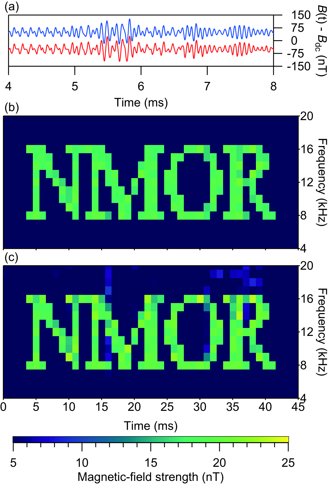
To highlight the wide bandwidth and large dynamic range of the technique we synthesized a magnetic field with a broad and dynamical spectrum that encodes the acronym ‘NMOR’ (nonlinear magneto-optical resonance). We drove the modulation coil with a wideband modulated current (see Fig. 6a), proportional to the resulting time-dependent field:
| (8) |
Here, we used the same dc magnetic field as displayed in Fig. 3 and Fourier components, each spaced by kHz, where kHz. The field amplitudes were piecewise constant, varying abruptly at 1 ms intervals to encode the acronym in the time-frequency domain. The resulting polarization rotation was of the form:
| (9) |
We retrieved the instantaneous phase from this measurand (Sec. II), and subtracted a linear fit (Sec. IV) to impute . The resulting oscillatory component of the instantaneous phase was analyzed in the time-frequency domain using the short-time Fourier transform (STFT). When the frequency binning is chosen to match , the STFT amplitudes are the time-dependent modulation indices mrad. The STFT amplitude was converted to magnetic field amplitudes and is displayed as a spectrogram on Fig. 6c. We compare this to the spectrogram of the intentionally applied field we predict at the sensor (Fig. 6b), based on the measured electrical current in the modulation coil and the Biot-Savart law. The two plots are in excellent agreement with only a small degradation in signal-to-noise ratio of the atomic magnetometer as approaches ms.
VI Discussion
Under the experimental conditions detailed here, the instantaneous phase of the polarization rotation has an observed noise floor of at frequencies above 100 Hz — within 60% of the shot-noise limit of (cf. App. C). This level of phase noise corresponds to a magnetic-field noise of approximately fT. All estimates of the modulation amplitude , modulation frequency , and carrier frequency presented here are within 15% of the Cramér-Rao lower bounds associated with this level of white phase noise Kay 1993.
For modulation frequencies below the carrier (), there is a single frequency component present in the retrieved instantaneous phase, at . However when (supra-carrier modulation), the oscillating component of the instantaneous phase retrieved using Eq. (4) contains two tones (cf. App. B), at and , with equal amplitudes . The frequency and amplitude of ac magnetic fields can still be imputed in the supra-carrier regime, provided we have knowledge of . This is guaranteed by the self-certifying estimate of , which is naturally obtained during linear regression to (Fig. 3). This is equally valid whether or .
The ability to measure high-frequency magnetic-field fluctuations will, in practice, depend upon the signal-to-noise ratio of the measurement. This can be thought of in two equivalent ways: the measured instantaneous-phase noise is white (independent of frequency), however the signal amplitude, when measured in rotation of the polarization, is given by the modulation index , which scales as . This results in a magnetic signal-to-noise ratio which also scales as . Alternatively, if we consider the signal amplitude in terms of the instantaneous-frequency then it is a constant value of ; however, the white instantaneous phase-noise considered in terms of frequency will be violet (differentiated white noise). Once again we see that the signal-to-noise ratio of an ac magnetic field measurement scales as .
The low-frequency response of this technique is limited to , below which the polarization-rotation signal will decay before a full modulation cycle has been observed. Of course, it would be possible to augment our technique with the traditional approach in which one uses repeated FID measurements: in this case, slow changes in can be tracked Hunter et al. 2018a.
We note that typical rf atomic magnetometers detect weak oscillating fields oriented transverse to the static background field Savukov et al. 2005; Lee et al. 2006; Ledbetter et al. 2007; Chalupczak et al. 2012; Savukov et al. 2014; Deans et al. 2018, whereas our magnetometer senses longitudinally oscillating fields. For arbitrarily oriented rf fields there will be a dead band of about the Larmor frequency, where a transverse component of the oscillating field with amplitude can drive Zeeman transitions, resulting in amplitude modulation of the polarization rotation Anderson et al. 2018.
VII Conclusion
We have developed a phase-retrieval technique that can extend the accuracy and applicability of dc optical atomic magnetometers so that they are now suitable for measuring ac magnetic fields. We explore a regime that was previously experimentally inaccessible, where the bandwidth of the sensor exceeds that of the Larmor frequency itself. We have demonstrated calibration-free measurement of oscillating fields in real time with amplitudes up to 150 nT, and frequencies up to 400 kHz, an increase in the amplitude and frequency response of two and three orders of magnitude over conventional rf atomic magnetometers respectively. The instantaneous-phase retrieval can be applied more broadly to quantum sensors that employ weak continuous measurement of spin precession, including those exploiting synchronous detection and feedback Vijay et al. 2012. This capability augurs well for robust field-deployable magnetometers which, unlike lab-based apparatus, face inherently unpredictable operational environments and transient signals of interest.
Acknowledgments
The authors acknowledge financial support from the Defence Science and Technology Group, and the South Australian Government through the Premier’s Science and Research Fund. N. W. and P. L. would like to thank Yvonne Stokes for useful discussions.
Appendix A Maximum Permissible Modulation Index
The frequency-modulated polarization rotation deriving from an oscillating magnetic field (Eq. 6) can be rewritten using the Jacobi-Anger expansion Korsch et al. 2006:
| (10) |
where is the -order Bessel function of the first kind. Thus, the polarization rotation comprises an infinite series of sidebands, distributed symmetrically about the carrier at , spaced by integer-multiples of the modulation frequency , with amplitudes .
A conservative upper bound for the maximum permissible modulation index, , is derived by considering the fractional power in sidebands about which extend to negative frequencies. These sidebands are discarded when numerically computing the analytic signal, which can compromise the instantaneous-phase retrieval. For a given fractional modulation frequency, , the largest value of such that , is given by:
| (11) |
To calculate for a given , one must choose an acceptable fractional power contained in the discarded sidebands. This constraint amounts to:
| (12) |
Using Bessel-function identities and symmetry relations, Eq. (12) simplifies to:
| (13) |
The maximum permissible modulation index calculated using Eq. (13) is shown in Fig. 7, for two different power fractions: and . Due to the nonlinearity of Eq. (13), an increasingly stringent bound on does not significantly reduce .
An additional constraint on arises from requiring that the instantaneous magnetic field never be zero, which could result in non-adiabatic spin-flips that compromise this measurement. This limits the maximum measurable ac magnetic-field amplitude to , equivalent to and thus . This constraint becomes stricter than the sideband-power considerations for .
Appendix B Instantaneous Phase Estimation when Modulating Faster Than the Carrier Frequency
For supra-carrier modulation (), the lower sideband nearest the positive-frequency carrier () at becomes negative ( in Eq. 10). When numerically computing the analytic signal in this regime, this sideband is discarded. However, due to the Hermitian symmetry of the Fourier transform of a real function, there is a corresponding upper sideband of the negative-frequency carrier () at which becomes positive. In the case of weak modulation (i.e. , which is generally the case when ), the majority of the modulated power of the analytic signal is contained in the two positive frequencies and . The spacing of these tones from the positive-frequency carrier is and , respectively. The asymmetry of these dominant sidebands results in a modification of the instantaneous phase retrieved using Eq. (4), in the form of double-sideband suppressed-carrier amplitude modulation:
| (14) | ||||
The resulting spectrum of contains two tones, at and . However, as the power is evenly distributed between these two tones, and the method prescribed in Fig. 3 can still be used to determine , the frequency and amplitude of ac magnetic fields can still be imputed unambiguously in the supra-carrier regime.
Appendix C Sensitivity
The magnetic sensitivity of this technique is ultimately determined by the ability to resolve small changes in the instantaneous phase. A representative amplitude spectral density of the instantaneous-phase is presented in Fig. 8, indicating a nearly white noise floor with magnitude . Using Eqs. (2) and (5), this level of instantaneous phase noise corresponds to a magnetic-field noise of .
A photocurrent-referenced measurement of the optical power indicates the shot-noise limit for instantaneous-phase is , or about in magnetic units.
References
- Bison et al. (2009) G. Bison, N. Castagna, A. Hofer, P. Knowles, J.-L. Schenker, M. Kasprzak, H. Saudan, and A. Weis, “A room temperature 19-channel magnetic field mapping device for cardiac signals,” Appl. Phys. Lett. 95, 173701 (2009).
- Bison et al. (2003a) G. Bison, R. Wynands, and A. Weis, “A laser-pumped magnetometer for the mapping of human cardiomagnetic fields,” Appl. Phys. B 76, 325–328 (2003a).
- Knappe et al. (2010) Svenja Knappe, Tilmann H. Sander, Olaf Kosch, Frank Wiekhorst, John Kitching, and Lutz Trahms, “Cross-validation of microfabricated atomic magnetometers with superconducting quantum interference devices for biomagnetic applications,” Appl. Phys. Lett. 97, 133703 (2010).
- Johnson et al. (2010) C. Johnson, P. D. D. Schwindt, and M. Weisend, “Magnetoencephalography with a two-color pump-probe, fiber-coupled atomic magnetometer,” Appl. Phys. Lett. 97, 243703 (2010).
- Xu et al. (2006) Shoujun Xu, Valeriy V. Yashchuk, Marcus H. Donaldson, Simon M. Rochester, Dmitry Budker, and Alexander Pines, “Magnetic resonance imaging with an optical atomic magnetometer,” Proc. Natl. Acad. Sci. U.S.A. 103, 12668–12671 (2006).
- Boto et al. (2018) Elena Boto, Niall Holmes, James Leggett, Gillian Roberts, Vishal Shah, Sofie S. Meyer, Leonardo Duque Muñoz, Karen J. Mullinger, Tim M. Tierney, Sven Bestmann, Gareth R. Barnes, Richard Bowtell, and Matthew J. Brookes, “Moving magnetoencephalography towards real-world applications with a wearable system,” Nature 555, 657–661 (2018).
- Jensen et al. (2018) K. Jensen, M. A. Skarsfeldt, H. Stærkind, J. Arnbak, M. V. Balabas, S.-P. Olesen, B. H. Bentzen, and E. S. Polzik, “Magnetocardiography on an isolated animal heart with a room-temperature optically pumped magnetometer,” Sci. Rep. 8, 16218 (2018).
- Belfi et al. (2007) J. Belfi, G. Bevilacqua, V. Biancalana, S. Cartaleva, Y. Dancheva, and L. Moi, “Cesium coherent population trapping magnetometer for cardiosignal detection in an unshielded environment,” J. Opt. Soc. Am. B 24, 2357–2362 (2007).
- Bison et al. (2003b) G. Bison, R. Wynands, and A. Weis, “Dynamical mapping of the human cardiomagnetic field with a room-temperature, laser-optical sensor,” Opt. Express 11, 904–909 (2003b).
- Xia et al. (2006) H. Xia, A. Ben-Amar Baranga, D. Hoffman, and M. V. Romalis, “Magnetoencephalography with an atomic magnetometer,” Appl. Phys. Lett. 89, 211104 (2006).
- Alem et al. (2015) O. Alem, T. H. Sander, R. Mhaskar, J. LeBlanc, H. Eswaran, U. Steinhoff, Y. Okada, J. Kitching, L. Trahms, and S. Knappe, “Fetal magnetocardiography measurements with an array of microfabricated optically pumped magnetometers,” Phys. Med. Biol. 60, 4797 (2015).
- Dang et al. (2010) H. B. Dang, A. C. Maloof, and M. V. Romalis, “Ultrahigh sensitivity magnetic field and magnetization measurements with an atomic magnetometer,” Appl. Phys. Lett. 97, 151110 (2010).
- Smiciklas et al. (2011) M. Smiciklas, J. M. Brown, L. W. Cheuk, S. J. Smullin, and M. V. Romalis, “New Test of Local Lorentz Invariance Using a 21Ne-Rb-K Comagnetometer,” Phys. Rev. Lett. 107, 171604 (2011).
- Berglund et al. (1995) C. J. Berglund, L. R. Hunter, D. Krause Jr., E. O. Prigge, M. S. Ronfeldt, and S. K. Lamoreaux, “New Limits on Local Lorentz Invariance from Hg and Cs Magnetometers,” Phys. Rev. Lett. 75, 1879 (1995).
- Pustelny et al. (2013) Szymon Pustelny, Derek F. Jackson Kimball, Chris Pankow, Micah P. Ledbetter, Przemyslaw Wlodarczyk, Piotr Wcislo, Maxim Pospelov, Joshua R. Smith, Jocelyn Read, Wojciech Gawlik, and Dmitry Budker, “The Global Network of Optical Magnetometers for Exotic physics (GNOME): A novel scheme to search for physics beyond the Standard Model,” Ann. Phys. 525, 659–670 (2013).
- Jackson Kimball et al. (2013) Derek F. Jackson Kimball, Ian Lacey, Julian Valdez, Jerlyn Swiatlowski, Cesar Rios, Rodrigo Peregrina-Ramirez, Caitlin Montcrieffe, Jackie Kremer, Jordan Dudley, and C. Sanchez, “A dual-isotope rubidium comagnetometer to search for anomalous long-range spin-mass (spin-gravity) couplings of the proton,” Ann. Phys. 525, 514–528 (2013).
- Schmelz et al. (2011) M Schmelz, R Stolz, V Zakosarenko, T Schönau, S Anders, L Fritzsch, M Mück, and H.-G. Meyer, “Field-stable SQUID magnetometer with sub-fT Hz-1/2 resolution based on sub-micrometer cross-type Josephson tunnel junctions,” Supercond. Sci. Technol. 24, 065009 (2011).
- Schönau et al. (2013) T. Schönau, M. Schmelz, V. Zakosarenko, R. Stolz, M. Meyer, S. Anders, L. Fritzsch, and H.-G. Meyer, “SQUID-based setup for the absolute measurement of the Earth’s magnetic field,” Supercond. Sci. Technol. 26, 035013 (2013).
- Kominis et al. (2003) I. K. Kominis, T. W. Kornack, J. C. Allred, and M. V. Romalis, “A subfemtotesla multichannel atomic magnetometer,” Nature 422, 596–599 (2003).
- Sheng et al. (2013) D. Sheng, S. Li, N. Dural, and M. V. Romalis, “Subfemtotesla Scalar Atomic Magnetometry Using Multipass Cells,” Phys. Rev. Lett. 110, 160802 (2013).
- Barry et al. (2016) John F. Barry, Matthew J. Turner, Jennifer M. Schloss, David R. Glenn, Yuyu Song, Mikhail D. Lukin, Hongkun Park, and Ronald L. Walsworth, “Optical magnetic detection of single-neuron action potentials using quantum defects in diamond,” Proc. Natl. Acad. Sci. U.S.A. 113, 14133–14138 (2016).
- Gerginov et al. (2017) V. Gerginov, F. C. S. da Silva, and D. Howe, “Prospects for magnetic field communications and location using quantum sensors,” Rev. Sci. Instrum. 88, 125005 (2017).
- (23) UK Defence Security Accelerator, Countering Drones – Finding and neutralising small UAS threats, April 2019.
- Savukov et al. (2005) I. M. Savukov, S. J. Seltzer, M. V. Romalis, and K. L. Sauer, “Tunable Atomic Magnetometer for Detection of Radio-Frequency Magnetic Fields,” Phys. Rev. Lett. 95, 063004 (2005).
- Ledbetter et al. (2007) M. P. Ledbetter, V. M. Acosta, S. M. Rochester, D. Budker, S. Pustelny, and V. V. Yashchuk, “Detection of radio-frequency magnetic fields using nonlinear magneto-optical rotation,” Phys. Rev. A 75, 023405 (2007).
- Chalupczak et al. (2012) W. Chalupczak, R. M. Godun, S. Pustelny, and W. Gawlik, “Room temperature femtotesla radio-frequency atomic magnetometer,” Appl. Phys. Lett. 100, 242401 (2012).
- Lee et al. (2006) S.-K. Lee, K. L. Sauer, S. J. Seltzer, O. Alem, and M. V. Romalis, “Subfemtotesla radio-frequency atomic magnetometer for detection of nuclear quadrupole resonance,” Appl. Phys. Lett. 89, 214106 (2006).
- Savukov et al. (2014) I. Savukov, T. Karaulanov, and M. G. Boshier, “Ultra-sensitive high-density Rb-87 radio-frequency magnetometer,” Appl. Phys. Lett. 104, 023504 (2014).
- Deans et al. (2018) Cameron Deans, Luca Marmugi, and Ferruccio Renzoni, “Sub-picotesla widely tunable atomic magnetometer operating at room-temperature in unshielded environments,” Rev. Sci. Instrum. 89, 083111 (2018).
- Rajroop (2018) Jenelle Rajroop, Radio-frequency atomic magnetometers: an analysis of interrogation regimes, PhD thesis, University College London (2018).
- Gawlik and Pustelny (2009) W. Gawlik and S. Pustelny, “New trends in quantum coherence and nonlinear optics,” (Nova Publishers, 2009) Chap. Nonlinear Faraday Effect and Its Applications, pp. 47–84.
- Gawlik and Pustelny (2017) W. Gawlik and S. Pustelny, “High Sensitvity Magnetometers,” in High sensitivity magnetometers (Springer, 2017) Chap. Nonlinear Magneto-Optical Rotation Magnetometers, pp. 425–450.
- Budker and Romalis (2007) D. Budker and M. Romalis, “Optical magnetometry,” Nat. Phys. 3, 227 (2007).
- Budker and Jackson Kimball (2013) D. Budker and D. F. Jackson Kimball, Optical magnetometry (Cambridge University Press, 2013).
- Jiménez-Martínez et al. (2012) R. Jiménez-Martínez, W. C. Griffith, S. Knappe, J. Kitching, and M. Prouty, “High-bandwidth optical magnetometer,” J. Opt. Soc. Am. B 29, 3398–3403 (2012).
- Pustelny et al. (2006) S. Pustelny, D. F. Jackson Kimball, S. M. Rochester, V. V. Yashchuk, and D. Budker, “Influence of magnetic-field inhomogeneity on nonlinear magneto-optical resonances,” Phys. Rev. A 74, 063406 (2006).
- Chaudhry (2014) Adam Zaman Chaudhry, “Utilizing nitrogen-vacancy centers to measure oscillating magnetic fields,” Phys. Rev. A 90, 042104 (2014).
- Baumgart et al. (2016) I. Baumgart, J.-M. Cai, A. Retzker, M. B. Plenio, and Ch. Wunderlich, “Ultrasensitive Magnetometer using a Single Atom,” Phys. Rev. Lett. 116, 240801 (2016).
- Anderson et al. (2018) R. P. Anderson, M. J. Kewming, and L. D. Turner, “Continuously observing a dynamically decoupled spin-1 quantum gas,” Phys. Rev. A 97, 013408 (2018).
- Cooper et al. (2014) A. Cooper, E. Magesan, H. N. Yum, and P. Cappellaro, “Time-resolved magnetic sensing with electronic spins in diamond,” Nat. Commun. 5, 3141 (2014).
- Puentes et al. (2014) Graciana Puentes, Gerald Waldherr, Philipp Neumann, Gopalakrishnan Balasubramanian, and Jörg Wrachtrup, “Efficient route to high-bandwidth nanoscale magnetometry using single spins in diamond,” Sci. Rep. 4, 4677 (2014).
- de Clercq et al. (2016) L. E. de Clercq, R. Oswald, C. Flühmann, B. Keitch, D. Kienzler, H.-Y. Lo, M. Marinelli, D. Nadlinger, V. Negnevitsky, and J. P. Home, “Estimation of a general time-dependent Hamiltonian for a single qubit,” Nat. Commun. 7, 11218 (2016).
- Boss et al. (2017) J. M. Boss, K. S. Cujia, J. Zopes, and C. L. Degen, “Quantum sensing with arbitrary frequency resolution,” Science 356, 837–840 (2017).
- Schmitt et al. (2017) Simon Schmitt, Tuvia Gefen, Felix M. Stürner, Thomas Unden, Gerhard Wolff, Christoph Müller, Jochen Scheuer, Boris Naydenov, Matthew Markham, Sebastien Pezzagna, Jan Meijer, Ilai Schwarz, Martin Plenio, Alex Retzker, Liam P. McGuinness, and Fedor Jelezko, “Submillihertz magnetic spectroscopy performed with a nanoscale quantum sensor,” Science 356, 832–837 (2017).
- Glenn et al. (2018) David R. Glenn, Dominik B. Bucher, Junghyun Lee, Mikhail D. Lukin, Hongkun Park, and Ronald L. Walsworth, “High-resolution magnetic resonance spectroscopy using a solid-state spin sensor,” Nature 555, 351–354 (2018).
- Martin Ciurana et al. (2017) F. Martin Ciurana, G. Colangelo, L. Slodička, R. J. Sewell, and M. W. Mitchell, “Entanglement-Enhanced Radio-Frequency Field Detection and Waveform Sensing,” Phys. Rev. Lett. 119, 043603 (2017).
- Jiménez-Martínez et al. (2018) Ricardo Jiménez-Martínez, Jan Kołodyński, Charikleia Troullinou, Vito Giovanni Lucivero, Jia Kong, and Morgan W. Mitchell, “Signal Tracking Beyond the Time Resolution of an Atomic Sensor by Kalman Filtering,” Phys. Rev. Lett. 120, 040503 (2018).
- Jasperse et al. (2017) M. Jasperse, M. J. Kewming, S. N. Fischer, P. Pakkiam, R. P. Anderson, and L. D. Turner, “Continuous Faraday measurement of spin precession without light shifts,” Phys. Rev. A 96, 063402 (2017).
- Bison et al. (2018) G. Bison, V. Bondar, P. Schmidt-Wellenburg, A. Schnabel, and J. Voigt, “Sensitive and stable vector magnetometer for operation in zero and finite fields,” Opt. Express 26, 17350–17359 (2018).
- Hunter et al. (2018a) Dominic Hunter, Ricardo Jiménez-Martínez, Juan Herbsommer, Srinath Ramaswamy, Wen Li, and Erling Riis, “Waveform reconstruction with a Cs based free-induction-decay magnetometer,” Opt. Express 26, 30523–30531 (2018a).
- Afach et al. (2015) S. Afach, G. Ban, G. Bison, K. Bodek, Z. Chowdhuri, Z. D. Grujić, L. Hayen, V. Hélaine, M. Kasprzak, K. Kirch, et al., “Highly stable atomic vector magnetometer based on free spin precession,” Opt. Express 23, 22108–22115 (2015).
- Grujić et al. (2015) Z. D. Grujić, P. A. Koss, G. Bison, and A. Weis, “A sensitive and accurate atomic magnetometer based on free spin precession,” Eur. Phys. J. D 69, 135 (2015).
- Hunter et al. (2018b) D. Hunter, S. Piccolomo, J. D. Pritchard, N. L. Brockie, T. E. Dyer, and E. Riis, “Free-induction-decay magnetometer based on a microfabricated Cs vapor cell,” Phys. Rev. Appl. 10, 014002 (2018b).
- Miao et al. (2019) P.-X. Miao, W.-Q. Zheng, S.-Y. Yang, B. Wu, B. Cheng, J.-H. Tu, H.-L. Ke, W. Yang, J. Wang, J.-Z. Cui, and L. Qiang, “Wide-range and self-locking atomic magnetometer based on free spin precession,” J. Opt. Soc. Am. B 36, 819–828 (2019).
- Wilson et al. (2019) Nathanial Wilson, Philip Light, André Luiten, and Christopher Perrella, “Ultrastable Optical Magnetometry,” Phys. Rev. Appl. 11, 044034 (2019).
- Alexandrov et al. (2005) E. B. Alexandrov, M. Auzinsh, D. Budker, D. F. Jackson Kimball, S. M. Rochester, and V. V. Yashchuk, “Dynamic effects in nonlinear magneto-optics of atoms and molecules,” J. Opt. Soc. Am. B 22, 7–20 (2005).
- (57) Although we establish an atomic alignment Budker et al. 2000 and subsequently track its precession, the technique described here would be equally applicable to extracting the instantaneous phase of an atomic orientation (oscillating about an carrier). We note that the use of an amplitude-modulated pump beam while establishing coherence and the relative orientation of the pump and probe beams are not critical elements of the technique reported here.
- Wilson et al. (2018) Nathanial Wilson, Nicolas Bourbeau Hébert, Christopher Perrella, Philip Light, Jérôme Genest, Szymon Pustelny, and André Luiten, “Simultaneous Observation of Nonlinear Magneto-Optical Rotation in the Temporal and Spectral Domains with an Electro-Optic Frequency Comb,” Phys. Rev. Appl. 10, 034012 (2018).
- Boashash (1992) B. Boashash, “Estimating and interpreting the instantaneous frequency of a signal. I. Fundamentals,” Proc. IEEE 80, 520–538 (1992).
- Barnes (1992) A. E. Barnes, “The calculation of instantaneous frequency and instantaneous bandwidth,” Geophysics 57, 1520–1524 (1992).
- (61) Daniel Adam Steck, “Rubidium 87 D Line Data,” http://steck.us/alkalidata, (revision 2.1.5, 13 September 2018).
- Kay (1993) S. M. Kay, Fundamentals of Statistical Signal Processing: Estimation Theory (Prentice Hall, 1993).
- Vijay et al. (2012) R. Vijay, C. Macklin, D. H. Slichter, S. J. Weber, K. W. Murch, R. Naik, A. N. Korotkov, and I. Siddiqi, “Stabilizing rabi oscillations in a superconducting qubit using quantum feedback,” Nature 490, 77–80 (2012).
- Korsch et al. (2006) H. J. Korsch, A. Klumpp, and D. Witthaut, “On two-dimensional bessel functions,” J. Phys. A: Math. Gen. 39, 14947 (2006).
- Budker et al. (2000) D. Budker, D. F. Jackson Kimball, S. M. Rochester, V. V. Yashchuk, and M. Zolotorev, “Sensitive magnetometry based on nonlinear magneto-optical rotation,” Phys. Rev. A 62, 043403 (2000).