Data-Driven Finite Elements Methods: Machine Learning Acceleration of Goal-Oriented Computations

To briefly illustrate our idea, let us consider a very simple motivating example. We consider the following simple 1-D elliptic boundary-value problem:

where $\delta_{\lambda}$ denotes the usual Dirac’s delta distribution centered at the point $\lambda\in(0,1)$. The quantity of interest (QoI) is the value $u_{\lambda}(x_{0})$ of the solution at some fixed point $x_{0}\in(0,1)$.

The standard variational formulation of problem (1) reads:

where $H_{(0}^{1}(0,1):=\{v\in L^{2}(0,1):v^{\prime}\in L^{2}(0,1)\wedge v(0)=0\}$. For the very coarse discrete subspace $\mathbb{U}_{h}:=\operatorname{Span}\{\psi\}\subset H_{(0}^{1}(0,1)$ consisting of the single linear trial function $\psi(x)=x$, the usual Galerkin method approximating (2) delivers the discrete solution $u_{h}(x)=\lambda x$. However, the exact solution to (1) is:

Hence, the relative error in the QoI for this case becomes:

As may be expected for this very coarse approximation, the relative errors are large (and actually never vanishes except in limiting cases).

Let us instead consider a Petrov–Galerkin method for (2), with the same trial space $\mathbb{U}_{h}$, but a special test space $\mathbb{V}_{h}$, i.e., $u_{h}\in\mathbb{U}_{h}:=\operatorname{Span}\{\psi\}$ such that $\int_{0}^{1}u_{h}^{\prime}v_{h}^{\prime}=v_{h}(\lambda)$, for all $v_{h}\in\mathbb{V}_{h}:=\operatorname{Span}\{\varphi\}$. We use the parametrized test function $\varphi(x)=\theta_{1}x+e^{-\theta_{2}}(1-e^{-\theta_{1}x})$, which is motivated by the simplest artificial neural network; see Section 4.1 for details. By varying the parameters $\theta_{1},\theta_{2}\in\mathbb{R}$, the errors in the quantity of interest can be significantly reduced. Indeed, Figure 1 shows the relative error in the QoI, plotted as a function of the $\theta_{1}$-parameter, with the other parameter set to $\theta_{2}=-9$, in the case of $x_{0}=0.1$ and two values of $\lambda$. When $\lambda=0.15>0.1=x_{0}$ (left plot in Figure 1), the optimal value $\theta_{1}\approx 48.5$ delivers a relative error of 0.575% in the quantity of interest. Notice that the Galerkin method has a relative error $>80\%$. For $\lambda=0.05<0.1=x_{0}$ (right plot in Figure 1), the value $\theta_{1}\approx 13.9$ actually delivers an exact approximation of the QoI, while the Galerkin method has a relative error $\approx 90\%$.

This example illustrates a general trend that we have observed in our numerical test (see Section 4): Striking improvements in quantities of interest are achieved using well-tuned test spaces.

Let us note that deep learning, in the form of artificial neural networks, has become extremely popular in scientific computation in the past few years, a crucial feature being the capacity of neural networks to approximate any continuous function [6]. While classical applications concern classification and prediction for image and speech recognition [14, 24, 18], there have been several new advances related to differential equations, either focussing on the data-driven discovery of governing equations [34, 3, 31] or the numerical approximation of (parametric) differential equations.

On the one hand, artificial neural networks can be directly employed to approximate a single PDE solution, see e.g. [2, 23, 25], and in particular the recent high-dimensional Ritz method [10]. On the other hand, in the area of model order reduction of differential equations, there have been tremendous recent developments in utilizing machine learning to obtain the reduced-order model for parametric models [19, 17, 33, 36, 22]. These developments are very closely related to recent works that use neural networks to optimize numerical methods, e.g., tuning the turbulence model [26], slope limiter [32] or artificial viscosity [9].

The idea of goal-oriented adaptive (finite element) methods date back to the late 1990s, see e.g., [1, 30, 28] for early works and analysis, and [13, 21, 38, 11, 16] for some recent new developments. These methods are based on a different idea than the machine-learning framework that we propose. Indeed, the classical goal-oriented methods aim to adaptively refine the underlying meshes (or spaces) so as to control the error in the quantity of interest, thereby adding more degrees of freedom at each adaptive step. In our framework, we train a finite element method so as to control the error in the quantity of interest based on training data for a parametric model. In particular, we do not change the number of degrees of freedom.

The contents of this paper are arranged as follows. Section 2 presents the machine-learning methodology to constructing data-driven finite element methods. It also presents the stability analysis of the discrete method as well as equivalent discrete formulations. Section 3 presents several implementational details related to artificial neural networks and the training procedure. Section 4 present numerical experiments for 1-D and 2-D elliptic and hyperbolic PDEs. Finally, Section 5 contains our conclusions.

We assume that the space $\mathbb{V}$ can be endowed with a family of equivalent weighted inner products $\{(\cdot,\cdot)_{\mathbb{V},\omega}\}_{\omega\in\mathcal{W}}$ and inherited norms $\{\|\cdot\|_{\mathbb{V},\omega}\}_{\omega\in\mathcal{W}}$, without affecting the topology given by the original norm $\|\cdot\|_{\mathbb{V}}$ on $\mathbb{V}$. That is, for each $\omega\in\mathcal{W}$, there exist equivalence constants $C_{1,\omega}>0$ and $C_{2,\omega}>0$ such that:

Consider a coarse finite dimensional subspace $\mathbb{U}_{h}\subset\mathbb{U}$ where we want to approximate the solution of (6), and let $\mathbb{V}_{h}\subset\mathbb{V}$ be a discrete test space such that $\dim{\mathbb{V}_{h}}\geq\dim\mathbb{U}_{h}$. The discrete method that we want to use to approach the solution $u_{\lambda}\in\mathbb{U}$ of problem (6), is to find $(r_{h,\lambda,\omega},u_{h,\lambda,\omega})\in\mathbb{V}_{h}\times\mathbb{U}_{h}$ such that:

System (8) corresponds to a residual minimization in a discrete dual norm that is equivalent to a Petrov–Galerkin method. See Section 2.3 for equivalent formulations and analysis of this discrete approach. In particular, the counterpart $r_{h,\lambda,\omega}\in\mathbb{V}_{h}$ of the solution of (8) is interpreted as a minimal residual representative, while $u_{h,\lambda,\omega}\in\mathbb{U}_{h}$ is the coarse approximation of $u_{\lambda}\in\mathbb{U}$ that we are looking for.

Assume now that one has a reliable sample set of $N_{s}\in\mathbb{N}$ (precomputed) data $\{(\lambda_{i},q(u_{\lambda_{i}}))\}_{i=1}^{N_{s}}$, where $q(u_{\lambda_{i}})$ is either the quantity of interest of the exact solution of (6) with $\lambda=\lambda_{i}\in\Lambda$, or else, a high-precision approximation of it. The main goal of this paper is to find a particular weight $\omega^{*}\in\mathcal{W}$, such that for the finite sample of parameters $\{\lambda_{i}\}_{i=1}^{N_{s}}\subset\Lambda$, the discrete solutions $\{u_{h,\lambda_{i},\omega^{*}}\}_{i=1}^{N_{s}}\subset\mathbb{U}_{h}$ of problem (8) with $\omega=\omega^{*}$, makes the errors in the quantity of interest as smallest as possible, i.e.,

To achieve this goal we will work with a particular family of weights described by artificial neural networks (ANN). The particular optimal weight $\omega^{*}$ will be trained using data-driven algorithms that we describe in the following. Our methodology will be divided into an expensive offline procedure (see Section 3.2) and an unexpensive online procedure (see Section 3.3).

In the offline procedure:

• •

  A weight function $\omega^{*}\in\mathcal{W}$ that minimizes (9) for a sample set of training data $\{(\lambda_{i},q(u_{\lambda_{i}}))\}_{i=1}^{N_{s}}$ is obtained.

• •

  From the matrix related with the discrete mixed formulation (8) using $\omega=\omega^{*}$, a static condensation procedure is applied to condense-out the residual variable $r_{h,\lambda,\omega^{*}}$. The condensed matrices are store for the online procedure.

In the online procedure:

• •

  The condensed mixed system (8) with $\omega=\omega^{*}$ is solved for multiple right-hand-sides in $\{\ell_{\lambda}\}_{\lambda\in\Lambda}$, and the quantities of interest $\{q(u_{h,\lambda,\omega^{*}})\}_{\lambda\in\Lambda}$ are directly computed as reliable approximations of $\{q(u_{\lambda})\}_{\lambda\in\Lambda}$.

In this section we analyze the well-posedness of the discrete system (8), as well as equivalent interpretations of it. The starting point will be always to assume well-posedness of the continuous (or infinite-dimensional) problem (6), which we will establish below.

The next Theorem 2.B establishes the well-posedness of the discrete mixed scheme (8).

The process of training an artificial neural network as (17) is performed by the minimization of a given functional $J(\Theta_{1},\phi_{1},\Theta_{2},\phi_{2},\dots,\Theta_{n},\phi_{n})$. We search for optimal sets of parameters $\{\Theta_{j}^{*}\}_{j=1}^{n}$ and $\{\phi_{j}^{*}\}_{j=1}^{n}$ minimizing the cost functional $J$. For simplicity, in what follows we will denote all the parameters of an artificial neural network by $\theta\in\Phi$, for a given set $\Phi$ of admissible parameters. A standard cost functional is constructed with a sample training set of known values $\{x_{1},x_{2},\dots,x_{N_{s}}\}$ and its corresponding labels $\{y_{1},y_{2},\dots,y_{N_{s}}\}$ as follows:

(for some real function $F$) which is known as supervised learning [14]. Training an artificial neural network means to solve the following minimization problem:

Thus, the artificial neural network evaluated in the optimal $\theta^{*}$ (i.e., $\operatorname{ANN}(x;\theta^{*})$) is the trained network. There are many sophisticated tailor-made procedures to perform the minimization in (19) efficiently. The reader may refer to [35] for inquiring into this topic, which is out of the scope of this paper.

The first step is to choose an artificial neural network $\operatorname{ANN}(\cdot\,;\theta)$ that will define a family $\mathcal{W}$ of positive weight-functions to be used in the weighted inner products $\{(\cdot,\cdot)_{\mathbb{V},\omega}\}_{\omega\in\mathcal{W}}$. Typically we have:

where $g$ is a suitable positive an bounded continuous function.

Next, given a discrete trial-test pairing $\mathbb{U}_{h}$-$\mathbb{V}_{h}$ satisfying (12), we construct the map $\mathcal{W}\times\Lambda\ni(\omega,\lambda)\mapsto q(u_{h,\lambda,\omega})\in\mathbb{R}$, where $u_{h,\lambda,\omega}\in\mathbb{U}_{h}$ is the second component of the solution the mixed system (8). Having coded this map, we proceed to train the $\operatorname{ANN}$ by computing:

The last step is to build the matrices of the linear system needed for the online phase. Denote the basis of $\mathbb{U}_{h}$ by $\{\psi_{1},...,\psi_{n}\}$, and the basis of $\mathbb{V}_{h}$ by $\{\varphi_{1},...,\varphi_{m}\}$ (recall that $m>n$). Having $\theta^{*}\in\Phi$ approaching (20), we extract from the mixed system (8) the matrices $A\in\mathbb{R}^{m\times m}$ and $B\in\mathbb{R}^{m\times n}$ such that:

where $\omega^{*}(\cdot)=g(\operatorname{ANN}(\cdot\,;\theta^{*}))$. Finally, we store the matrices $B^{T}A^{-1}B\in\mathbb{R}^{n\times n}$ and $B^{T}A^{-1}\in\mathbb{R}^{n\times m}$ to be used in the online phase to compute directly $u_{h,\lambda,\omega^{*}}\in\mathbb{U}_{h}$ for any right hand side $\ell_{\lambda}\in\mathbb{V}^{*}$. Basically, we have condensed-out the residual variable of the mixed system (8), since it is useless for the application of the quantity of interest $q\in\mathbb{U}^{*}$. In addition, it will be also important to store the vector $Q\in\mathbb{R}^{n}$ such that:

For each $\lambda\in\Lambda$ for which we want to obtain the quantity of interest $q(u_{h,\lambda,\omega^{*}})$, we first compute the vector $L_{\lambda}\in\mathbb{R}^{m}$ such that its $i$-th component is given by:

where $\varphi_{i}$ is the $i$-th vector of in the basis of $\mathbb{V}_{h}$. Next, we compute

Observe that the matrix $Q^{T}(B^{T}A^{-1}B)^{-1}B^{T}A^{-1}$ can be fully obtained and stored from the previous offline phase (see Section 3.2).

We recover here the motivational example from the introduction (see Section 1.1). Consider the variational formulation (2), with trial and test spaces $\mathbb{U}=\mathbb{V}=H_{(0}^{1}(0,1)$. We endowed $\mathbb{V}$ with the weighted inner product:

As in the introduction, we consider the simplest coarse discrete trial space $\mathbb{U}_{h}:=\operatorname{Span}\{\psi\}\subset\mathbb{U}$, where $\psi(x)=x$. The optimal test function (see Section 2.3.1), paired with the trial function $\psi$, is given by $\varphi:=T_{\omega}\psi\in\mathbb{V}$, which is the solution of (14) with $u=\psi$. Hence,

Let us consider the Petrov-Galerkin formulation with optimal test functions, which is equivalent to the mixed system (8) in the optimal case $\mathbb{V}_{h}=\mathbb{V}$. Consequently, the Petrov-Galerkin scheme with trial function $\psi$ and optimal test function $\varphi$, delivers the discrete solution $u_{h,\lambda,\omega}(x)=x\varphi(\lambda)/\varphi(1)$ (notice that the trivial weight $\omega\equiv 1$ recovers the test function $\varphi=\psi$, and therefore the standard Galerkin approach).

Recalling the exact solution (3), we observe that the relative error in the quantity of interest for our Petrov-Galerkin approach is:

Of course, any function such that $\varphi(\lambda)=\varphi(x_{0})\neq 0$ for $\lambda\geq x_{0}$, and $\varphi(\lambda)=\lambda\varphi(x_{0})/x_{0}$ for $\lambda\leq x_{0}$, will produce zero error for all $\lambda\in(0,1)$. Notice that such a function indeed exists, and in this one-dimensional setting it solves the adjoint problem:

This optimal test function is also obtained in our framework via (21), by using a limiting weight of the form:

for some constant $c>0$. Hence, the Petrov–Galerkin method using a test function of the form (21) has sufficient variability to eliminate any errors for any $\lambda$!

We now restrict the variability by parametrizing $\omega$. In the motivating example given in Section 1.1, for illustration reasons we chose a weight of the form $\omega(x)=\sigma(\theta_{1}x+\theta_{2})$, which corresponds to the most simple artificial neural network, having only one hidden layer with one neuron. We now select a slightly more complex family of weights having the form $\omega(x)=\exp(\operatorname{ANN}(x;\theta))>0$, where

Observe that $\operatorname{ANN}(x;\theta)$ corresponds to an artificial neural network of one hidden layer with five neurons (see Section 3.1).

The training set of parameters has been chosen as $\lambda_{i}=0.1i$, with $i=1,...,9$. For comparisons, we perform three different experiments. The first experiment trains the network (24) based on a cost functional that uses the relative error formula (22), where the optimal test function $\varphi$ is computed using eq. (21). The other two experiments use the training approach (20), with discrete spaces $\mathbb{V}_{h}$ consisting of conforming piecewise linear functions over uniform meshes of 4 and 16 elements respectively. The quantity of interest has been set to $x_{0}=0.6$, which does not coincide with a node of the discrete test spaces. Figure 2 shows the obtained discrete solutions $u_{h,\lambda,\omega^{*}}$ for each experiment, and for two different values of $\lambda$. Figure 3(a) shows the trained weight obtained for each experiment (cf. eq. (23)), while Figure 3(b) depicted the associated optimal and projected-optimal test functions linked to those trained weights. Finally, Figure 3(c) shows the relative errors in the quantity of interest for each discrete solution in terms of the $\lambda$ parameter.

It can be observed that the trained method using a parametrized weight function based on (24), while consisting of only one degree of freedom, gives quite accurate quantities of interest for the entire range of $\lambda$. This should be compared to the $O(1)$ error for standard Galerkin given by (4). We note that some variation can be observed depending on whether the optimal or a projected optimal test function is used (with a richer $\mathbb{V}_{h}$ being better).

Consider the family of ODEs:

for a family of continuous functions $\{f_{\lambda}\}_{\lambda\in[0,1]}$ given by $f_{\lambda}(x):=(x-\lambda)\mathbbm{1}_{[\lambda,1]}(x)$, where $\mathbbm{1}_{[\lambda,1]}$ denote the characteristic function of the interval $[\lambda,1]$. The exact solution of (25) will be used as a reference solution and is given by $u_{\lambda}(x)={1\over 2}(x-\lambda)^{2}\mathbbm{1}_{[\lambda,1]}(x)$. The quantity of interest considered for this example will be $q_{x_{0}}(u_{\lambda}):=u_{\lambda}(x_{0})$, where $x_{0}$ could be any value in $[0,1]$.

Let us consider the following variational formulation of problem (25):

where $\mathbb{U}:=H^{1}_{(0}(0,1):=\{u\in L^{2}(0,1):u^{\prime}\in L^{2}(0,1)\wedge u(0)=0\}$, and $\mathbb{V}:=L^{2}(0,1)$ is endowed with the weighted inner-product:

We want to approach this problem using coarse discrete trial spaces $\mathbb{U}_{h}\subset\mathbb{U}$ of piecewise linear polynomials on a partition of one, two and three elements.

We describe the weight $\omega(x)$ by the sigmoid of an artificial neural network that depends on parameters $\theta$, i.e., $\omega(x)=\sigma(\mathrm{ANN}(x;\theta))>0$ (see Section 3.1). In particular, we use the artificial neural network given in (24). To train such a network, we consider a training set $\{\lambda_{i}\}_{i=1}^{9}$, where $\lambda_{i}=0.125(i-1)$, together with the set of exact quantities of interest $\{q_{x_{0}}(u_{\lambda_{i}})\}_{i=1}^{9}$, computed using the reference exact solution with $x_{0}=0.9$. The training procedure uses the constrained minimization problem (20), where for each low-resolution trial space $\mathbb{U}_{h}$ (based on one, two and three elements), the same discrete test space $\mathbb{V}_{h}$ has been used: a high-resolution space of piecewise linear and continuous functions linked to a uniform partition of 128 elements. The minimization algorithm has been stopped until the cost functional reaches the tolerance tol$=9\cdot 10^{-7}$.

After an optimal parameter $\theta^{*}$ has been found (see (20)), we follow the matrix procedures described in Section 3.2 and Section 3.3 to approach the quantity of interest of the discrete solution for any $\lambda\in[0,1]$.

Figures 4 and 5 show numerical experiments considering model problem (25) in three different trial spaces. Figure 4 shows, for $\lambda=0.19$, the exact solution and the Petrov-Galerkin solution computed with projected optimal test functions given by the trained weighted inner-product. Notice that for the three cases (with one, two, and three elements) the Petrov-Galerkin solution intends to approximate the quantity of interest (dotted line).

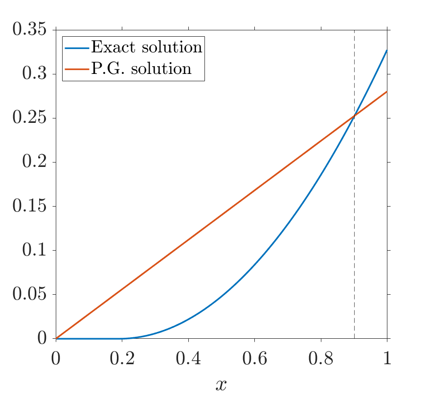
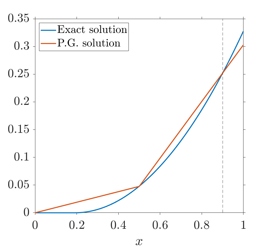
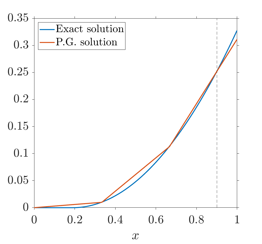
Figure 5 displays the QoI error $|q_{x_{0}}(u_{\lambda})-q_{x_{0}}(u_{\lambda,h,\omega^{*}})|$ for different values of $\lambda\in[0,1]$. When the ANN-training stops at a cost functional smaller than tol$=9\cdot 10^{-7}$, the QoI error remains smaller than $10^{-3}$ for all $\lambda\in[0.1]$. In particular, Figure 5(a) shows that even in the simplest case of one-degree of freedom, it is possible to get reasonable approximations of the QoI for the entire range of $\lambda$.

This example is based on the same model problem of Section 4.2, but now we intend to approach two quantities of interest simultaneously: $q_{1}(u_{\lambda}):=u_{\lambda}(x_{1})$ and $q_{2}(u_{\lambda}):=u_{\lambda}(x_{2})$, where $x_{1},x_{2}\in[0,1]$ are two different values. We also have considered now discrete trial spaces based on three, four and five elements. The training routine has been modified accordingly, and is driven now by the following minimization problem:

For this example, we consider a training set of size $N_{s}=12$ with $\lambda_{i}=(i-1)/11$, for all $i=1,\dots,12$. The weight $\omega(x)$ will be described by the sigmoid of an artificial neural network that depends on one single hidden layer and $N_{n}=6$ hidden neurons. Numerical results are depicted in Figures 6 and 7 for $x_{1}=0.3$ and $x_{2}=0.7$. Accurate values of both QoIs are obtained for the entire range of $\lambda$. These results are roughly independent of the size of the trial space.

Consider the two-dimensional unit square $\Omega=[0,1]\times[0,1]$ and the family of PDEs:

where the family of functions $\{f_{\lambda}\}_{\lambda\in(0,1)}$ is described by the formula:

Accordingly, the reference exact solution of (26) is:

The quantity of interest chosen for this example will be the average

References

- [1] R. Becker and R. Rannacher, An optimal control approach to a posteriori error estimation in finite element methods, Acta Numer., 10 (2001), pp. 1–102.
- [2] J. Berg and K. Nyström, A unified deep artificial neural network approach to partial differential equations in complex geometries, Neurocomputing, 317 (2018), pp. 28–41.
- [3] J. Berg and K. Nyström, Data-driven discovery of PDEs in complex datasets, Journal of Computational Physics, 384 (2019), pp. 239–252.
- [4] D. Broersen and R. Stevenson, A robust Petrov–Galerkin discretisation of convection–diffusion equations, Comput. Math. Appl., 68 (2014), pp. 1605–1618.
- [5] J.-T. Chien, Source separation and machine learning, Academic Press, 2018.
- [6] G. Cybenko, Approximation by superpositions of a sigmoidal function, Mathematics of Control, Signals, and Systems, 2 (1989), pp. 303–314.
- [7] L. Demkowicz and J. Gopalakrishnan, A class of discontinuous Petrov-Galerkin methods. II. Optimal test functions, Numerical Methods for Partial Differential Equations, 27 (2010), pp. 70–105.
- [8] L. Demkowicz and J. Gopalakrishnan, An overview of the discontinuous Petrov Galerkin method, in Recent Developments in Discontinuous Galerkin Finite Element Methods for Partial Differential Equations: 2012 John H Barrett Memorial Lectures, X. Feng, O. Karakashian, and Y. Xing, eds., vol. 157 of The IMA Volumes in Mathematics and its Applications, Springer, Cham, 2014, pp. 149–180.
- [9] N. Discacciati, J. S. Hesthaven, and D. Ray, Controlling oscillations in high-order Discontinuous Galerkin schemes using artificial viscosity tuned by neural networks, To appear in J. Comput. Phys (2020), (2020).
- [10] W. E and B. Yu, The deep Ritz method: A deep learning-based numerical algorithm for solving variational problems, Commun. Math. Stat., 6 (2018), pp. 1–12.
- [11] B. Endtmeyer and T. Wick, A partition-of-unity dual-weighted residual approach for multi-objective goal functional error estimation applied to elliptic problems, Comput. Methods Appl. Math., 17 (2017), pp. 575–600.
- [12] A. Ern and J.-L. Guermond, Theory and practice of finite elements, Springer, New-York, 2004.
- [13] M. Feischl, D. Praetorius, and K. G. van der Zee, An abstract analysis of optimal goal-oriented adaptivity, SIAM J. Numer. Anal., 54 (2016), pp. 1423–1448.
- [14] I. Goodfellow, Y. Bengio, and A. Courville, Deep Learning, The MIT Press, 2019.
- [15] J. Gopalakrishnan and W. Qiu, An analysis of the practical DPG method, Math. Comp., 83 (2014), pp. 537–552.
- [16] B. Hayhurst, M. Keller, C. Rai, X. Sun, and C. R. Westphal, Adaptively weighted least squares finite element methods for partial differential equations with singularities, Comm. Applied Math. and Comput. Science, 13 (2018), pp. 1–25.
- [17] J. S. Hesthaven and S. Ubbiali, Non-intrusive reduced order modeling of nonlinear problems using neural networks, J. Comput. Phys., 363 (2018), pp. 55–78.
- [18] C. F. Higham and D. J. Higham, Deep learning: An introduction for applied mathematicians, SIREV, 61 (2019), pp. 860–891.
- [19] A. C. Ionita and A. C. Antoulas, Data-driven parametrized model reduction in the Lowner framework, SIAM Journal of Scientific Computing, 36 (2014), pp. A984–A1007.
- [20] T. Kato, Estimation of iterated matrices with application to von Neumann condition, Numer. Math., 2 (1960), pp. 22–29.
- [21] K. Kergrene, S. Prudhomme, L. Chamoin, and M. Laforest, A new goal-oriented formulation of the finite element method, Comput. Methods Appl. Mech. Engrg., 327 (2017), pp. 256–276.
- [22] G. Kutyniok, P. Petersen, M. Raslan, and R. Schneider, A theoretical analysis of deep neural networks and parametric PDEs, arXiv preprint, arXiv:1904.00377v2 (2019).
- [23] I. Lagaris, A. Likas, and D. Fotiadis, Artificial neural networks for solving ordinary and partial differential equations, IEEE Transactions on Neural Networks, 9 (1998), pp. 987–1000.
- [24] Y. LeCun, Y. Bengio, and G. Hinton, Deep learning, Nature, 521 (2015), pp. 436–444.
- [25] H. Lee and I. S. Kang, Neural algorithm for solving differential equations, Journal of Computational Physics, 91 (1990), pp. 110–131.
- [26] J. Ling, A. Kurzawski, and J. Templeton, Reynolds averaged turbulence modelling using deep neural networks with embedded invariance, J. Fluid Mech., 807 (2016), pp. 155–166.
- [27] S. Mishra, A machine learning framework for data driven acceleration of computations of differential equations, Mathematics in Engineering, 1 (2018), pp. 118–146.
- [28] M. S. Mommer and R. Stevenson, A goal-oriented adaptive finite element method with convergence rates, SIAM J. Numer. Anal., 47 (2009), pp. 861–886.
- [29] I. Muga and K. G. van der Zee, Discretization of linear problems in Banach spaces: Residual minimization, nonlinear Petrov–Galerkin, and monotone mixed methods. http://arxiv.org/abs/1511.04400, 2018.
- [30] J. T. Oden and S. Prudhomme, Goal-oriented error estimation and adaptivity for the finite element method, Comput. Math. Appl., 41 (2001), pp. 735–756.
- [31] M. Raissi and G. E. Karniadakis, Hidden physics models: Machine learning of nonlinear partial differential equations, J. Comput. Phys., 357 (2018), pp. 125–141.
- [32] D. Ray and J. S. Hesthaven, An artificial neural network as a troubled-cell indicator, J. Comput. Phys., 367 (2018), pp. 166–191.
- [33] F. Regazzoni, L. Dedè, and A. Quarteroni, Machine learning for fast and reliable solution of time-dependent differential equations, Journal of Computational Physics, 397 (2019), p. 108852.
- [34] S. H. Rudy, S. L. Brunton, J. L. Proctor, and J. N. Kutz, Data-driven discovery of partial differential equations, Science Advances, 3 (2017), p. e1602614.
- [35] S. Sra, S. Nowozin, and S. J. Wright, Optimization for machine learning, The MIT Press, 2011.
- [36] R. Swischuka, L. Maininia, B. Peherstorferb, and K. Willcox, Projection-based model reduction: Formulations for physics-based machine learning, Computers and Fluids, 179 (2019), pp. 704–717.
- [37] G. Tsihrintzis, D. N. Sotiropoulos, and L. C. Jain, Machine learning paradigms: Advances in data analytics, Springer, 2019.
- [38] E. H. van Brummelen, S. Zhuk, and G. J. van Zwieten, Worst-case multi-objective error estimation and adaptivity, Comput. Methods Appl. Mech. Engrg., 313 (2017), pp. 723–743.