A tale of two sites - I: Inferring the properties of minihalo-hosted galaxies from current observations
Abstract
The very first galaxies that started the cosmic dawn likely resided in so-called “minihaloes”, with masses of –, accreting their gas from the intergalactic medium through H2 cooling. Such molecularly cooled galaxies (MCGs) mostly formed in pristine environments, hosted massive, metal-free stars, and were eventually sterilized by the build-up of a disassociating (Lyman–Werner; LW) background. Therefore, their properties might be very different from the galaxies we see in the later Universe. Although MCGs are probably too faint to be observed directly, we could nevertheless infer their properties from the imprint they leave in the cosmic 21-cm signal. Here we quantify this imprint by extending the public simulation code 21cmFAST to allow for a distinct population of MCGs. We allow MCGs to have different properties from other galaxies, including unique scaling relations for their stellar-to-halo mass ratios, ionizing escape fractions, and spectral energy distributions. We track inhomogeneous recombinations, disassociative LW feedback, and photoheating from reionization. After demonstrating how MCGs can shape the 21-cm signal, we explore to what extent current observations can already place constraints on their properties. The cosmic microwave background optical depth from Planck sets an upper limit on the product of the ionizing escape fraction and the stellar mass in MCGs. When including also the timing of the putative EDGES absorption signal, we find an additional strong degeneracy between the stellar mass and the X-ray luminosity of MCGs. If proven to be of cosmic origin, the timing of the EDGES signal would have been set by MCGs.
Keywords:
galaxies: high-redshift; intergalactic medium; dark ages, reionization, first stars; diffuse radiation; early Universe; cosmology: theory1 Introduction
The hyperfine spin-flip transition of neutral hydrogen, corresponding to a photon with a wavelength of 21 cm, promises to revolutionize our understanding of the first billion years of the Universe. The cosmic 21-cm signal is typically expressed as the brightness temperature contrast of the cosmic hydrogen against the cosmic microwave background (CMB), at a redshifted frequency and spatial position (e.g. Furlanetto et al. 2006)
| (1) |
where is the CMB temperature; is the spin temperature denoting the relative level populations of the hyperfine transition; is the Hubble constant at redshift ; and is the optical depth and is a function of the spin temperature, neutral hydrogen fraction (), local overdensity ( with and being the baryonic density and its cosmic mean, respectively), and the line-of-sight velocity gradient (d/d), as well as cosmological parameters, such as the present baryon and matter abundances, and , and the Hubble constant, .
In addition to physical cosmology, the signal is sensitive to the ionization and thermal state of the intergalactic medium (IGM), which are governed by the ionizing, X-ray and soft UV radiation fields during the cosmic dawn (CD) and subsequent epoch of reionization (EoR). These radiation fields are established by stars and black holes inside the first generations of galaxies (though exotic sources such as dark matter annihilation or primordial black holes might contribute; e.g. Evoli et al. 2014; Lopez-Honorez et al. 2016; Hektor et al. 2018). Thus, the cosmic 21-cm signal encodes the properties of unseen galaxies during the first billion years. Current interferometers, including the Low-Frequency Array (LOFAR11 1 http://www.lofar.org/; van Haarlem et al. 2013; Patil et al. 2017) and the Murchison Widefield Array (MWA22 2 http://www.mwatelescope.org/; Tingay et al. 2013; Beardsley et al. 2016), are aiming for a statistical detection of the EoR; however, next-generation instruments, such as the Hydrogen Epoch of Reionization Arrays (HERA33 3 http://reionization.org/; DeBoer et al. 2017; Kohn et al. 2019) and the Square Kilometre Array (SKA44 4 https://www.skatelescope.org/; Mellema et al. 2013; Koopmans et al. 2015), are expected to characterize the topology of the CD, allowing us to indirectly study the very first galaxies out to –30.
The first generations of galaxies are expected to reside in so-called minihaloes, with virial temperatures below K. At these low temperatures, cooling through atomic hydrogen () and helium (He) is inefficient; therefore, minihaloes obtain gas from the IGM and cool predominately through molecular hydrogen () cooling (e.g. Haiman et al. 1996; Haiman et al. 1997; Yoshida et al. 2003; Yoshida et al. 2006). As they form out of pristine (unpolluted) gas, these minihaloes or molecular-cooling galaxies (MCGs) are expected to host metal-free (so-called PopIII) stars and associated remnants (Wise et al. 2012; Xu et al. 2016). Their shallow potential wells suggest that they are sensitive to supernova and photoheating feedback (Haiman et al. 2000; Wise & Abel 2007; Kimm et al. 2017). Moreover, star formation inside MCGs is expected to be transient since an H2-disassociating (Lyman–Werner; LW) background becomes established soon after the first stars form (e.g. Johnson et al. 2007; Ahn et al. 2009; Holzbauer & Furlanetto 2012; Fialkov et al. 2013; Jaacks et al. 2019; Schauer et al. 2019). Because of this uniqueness (pristine environment, top-heavy initial mass function (IMF), transient star formation, peculiar energetics), it is doubtful that the typical properties of MCGs can be adequately captured by simply extending the scaling relations inferred from observations of their massive counterparts at lower redshifts (e.g. Mirocha & Furlanetto 2019; Mebane et al. 2020).
Unfortunately, studying MCGs through direct observations is unlikely in the foreseeable future. Most are expected to have UV magnitudes in the range of -5 to -12 (e.g. O’Shea et al. 2015; Xu et al. 2016), below the observational limit of even the next-generation infrared instrument, the James Webb Space Telescope (JWST; Gardner et al. 2006). Gravitational lensing has allowed us to push UV luminosity functions (LFs) down to at (e.g. Bouwens et al. 2017; Livermore et al. 2017; Atek et al. 2018; Ishigaki et al. 2018). However, even if the associated large systematic uncertainties can be mitigated, MCGs seem unlikely to persist at these low redshifts and few if any might be found in the effective lensing volume (e.g. Atek et al. 2018).
Thankfully, these transient first galaxies leave an imprint in the timing and topology of the 21-cm signal. For example, massive stars in MCGs could be responsible for a tail in the reionization history extending towards high redshifts (e.g. Ahn et al. 2012; Visbal et al. 2015; Miranda et al. 2017), and imprint more small-scale structure in the reionization topology (e.g. Mesinger et al. 2012; Koh & Wise 2018), while the neutral gas inside minihaloes can act as ionizing photon sinks, delaying reionization and further affecting the topological features (e.g. Ciardi et al. 2006; McQuinn et al. 2007). MCGs could play an even more prominent role in the timing and morphology of the earlier epochs when X-rays and soft UV photons drive the 21-cm signal (e.g. Fialkov et al. 2013; Fialkov & Barkana 2014; Mirocha et al. 2018; Muñoz 2019a; Mebane et al. 2020). Indeed, these early epochs recently received attention because of the claimed detection of the globally averaged 21-cm absorption feature at by the Experiment to Detect the Global Epoch of Reionization Signature (EDGES; Bowman et al. 2018). Although the cosmological interpretation of the EDGES result remains controversial (e.g. Hills et al. 2018; Bradley et al. 2019; Sims & Pober 2019), if the signal is indeed proven to be of cosmic origins, X-rays and soft UV radiation from MCGs were likely responsible for its timing (e.g. Mirocha & Furlanetto 2019).
In this work, we explore the imprints of MCGs in the 21-cm signal from the EoR and CD, introducing a distinct population in the public code 21cmFAST(Mesinger & Furlanetto 2007; Mesinger et al. 2011), whose abundance is regulated by an H2-disassociating background (see also Fialkov et al. 2013; Muñoz 2019a). We build upon the model of Park et al. 2019, whose parametrization allows star formation rates (SFRs) to scale non-linearly with the mass of the host halo, thus allowing the source models to be consistent with current UV LF observations (e.g. Hassan et al. 2016; Mirocha et al. 2016; Mutch et al. 2016). We extend this model, allowing MCGs to have their own unique properties, including star formation efficiencies, ionizing escape fractions, and X-ray and soft UV emissivities. By varying the free parameters in our model, we quantify how the diverse properties of two galaxy populations (atomic and molecular cooling) are imprinted in the global and interferometric 21-cm signals. As a proof of concept, we confront this extended two-population model with the putative EDGES detection, using its timing to constrain the properties of minihalo-hosted galaxies within a Bayesian framework, 21CMMC55 5 https://github.com/BradGreig/21CMMC (Greig & Mesinger 2015). The code developed for this work will be part of the upcoming v3.0.0 release of 21cmFAST66 6 https://github.com/21cmfast/21cmFAST.
This paper is organized as follows. We present our model in Section 2. In Section 3, we investigate the impact of the physical properties of our model on the 21-cm signal. In Section 4 we perform a Monte Carlo Markov Chain (MCMC) with a subset of model parameters, showing constraints available with and without the EDGES result. Finally, we conclude in Section 5. In this work, we use a CDM cosmology with parameters and = (0.31, 0.048, 0.69, 0.68, 0.81, and 0.97, consistent with results from the Planck satellite (e.g. Planck Collaboration et al. 2016b).
2 Modelling galaxies, the IGM, and cosmic radiation fields
2.1 Star formation and galaxy evolution
As gas from the IGM accretes onto dark matter halos, its gravitational potential energy is converted into heat. In order to avoid becoming pressure supported and continue collapsing onto the galaxy at the centre of the halo, gas needs to cool by emitting radiation that must escape the system. Galaxies can be classified by the dominant cooling channel through which the IGM gas has been accreted onto the halo: (i) atomic-cooling galaxies (ACGs), which predominantly obtained their gas through (and He) line transitions efficient at virial temperatures () above ; and (ii) MCGs, in which the gas cools mainly through the rotational–vibrational transitions efficient at ; most ACGs at high redshifts are “second-generation” galaxies, forming out of MCG building blocks. The pre-enrichment by metals as well as the different energetics and cooling processes suggests that the stellar component and interstellar medium (ISM) of ACG and MCG should have different properties. As these properties are currently poorly understood, we describe them through relatively generic and flexible parametric models. Next, we introduce these for both ACGs and MCGs.
2.1.1 Atomic-cooling galaxies
“Massive” ACGs (; e.g. Kuhlen & Faucher-Giguère 2012; Mason et al. 2015; Liu et al. 2016) have been observed by the Hubble Space Telescope (HST). The resulting non-ionizing UV LFs (e.g. Bouwens et al. 2015; Bouwens et al. 2016; Finkelstein et al. 2015; Livermore et al. 2017; Atek et al. 2018; Oesch et al. 2018; Bhatawdekar et al. 2019) give invaluable insight into star formation processes inside these galaxies, ruling out the constant mass-to-light ratio models commonly found in early 21-cm forecasts (e.g. Mesinger et al. 2011; Fialkov et al. 2013).
Here we build upon the model of Park et al. 2019, which is flexible enough to reproduce observed high-redshift LFs. This simple model describes the ACG population through power-law scaling relations with the halo mass function (HMF; see also Kuhlen & Faucher-Giguère 2012; Mitra et al. 2015; Sun & Furlanetto 2016; Behroozi et al. 2019) Although individual galaxies have much more complicated and stochastic evolution of properties (e.g. Mutch et al. 2016; Ma et al. 2018; Yung et al. 2019), the 21-cm signal on observable scales () is sourced by hundreds of galaxies, motivating the use of simple and computationally efficient average scaling relations.
Specifically, we describe the stellar mass of an ACG, , hosted in a halo with a mass of by
| (2) |
where and are the normalization factor and power-law index. More detailed models recover such scaling relations for the bulk of the high-redshift galaxy population (e.g. Moster et al. 2013; Mutch et al. 2016; Sun & Furlanetto 2016; Tacchella et al. 2018; Behroozi et al. 2019; Yung et al. 2019). Note that we do not consider AGN feedback, which is thought to dominate in the most massive galaxies, as these are too rare at high redshifts to shape the 21-cm signal (e.g. Mitra et al. 2015; Manti et al. 2017; Parsa et al. 2017; Qin et al. 2017; Ricci et al. 2017; Garaldi et al. 2019). We also do not include a redshift evolution in this stellar-to-halo mass relation, which is supported by some simulation results (e.g. Mutch et al. 2016; Xu et al. 2016), although generalizing the model to include a redshift evolution is trivial.
The corresponding average SFR is assumed to be
| (3) |
where is a free parameter corresponding to the typical star formation time-scale, defined as a fraction of the Hubble time. Since the dynamical time of a halo scales with the Hubble time during matter domination, this is analogous to assuming the star formation time scales with the dynamical time.
We include an exponential duty cycle77 7 The duty cycle is defined as the fraction of halos that harbour star-forming galaxies for a given halo mass. It is used to describe the stochasticity of star formation and can be considered as an occupation fraction (e.g. Lippai et al. 2009; Miller et al. 2015). to describe the mass function of halos (HMF) that host star-forming ACGs
| (4) |
where is the mass function of all halos. The exponential term in equation (4) accounts for inefficient star formation in halos below a characteristic mass scale (i.e. turnover mass)
| (5) |
As can be seen from equation (5), we assume that star formation in small ACGs can be limited by three physical processes: (i) inefficient cooling, ; (ii) photoheating feedback from reionization, ; and (iii) supernova feedback, .
For (i), we assume the cooling threshold to be 104K. The corresponding halo mass can be expressed as (e.g. Barkana & Loeb 2001)
| (6) |
where is the mean molecular weight, is the critical overdensity of halos at collapse in the spherical collapse model, and is the matter density in units of the critical density at redshift .
For photoheating feedback inside reionized regions of the Universe (ii; see Efstathiou 1992; Shapiro et al. 1994; Thoul & Weinberg 1996; Hui & Gnedin 1997; Dijkstra et al. 2004), we take the functional form from Sobacchi & Mesinger 2014
| (7) |
where and are the local photoionization rate and the redshift at which the local patch of the IGM was reionized, respectively; the factor accounts for the enhanced photoionization rate at galaxy locations due to their clustering (Mesinger & Dijkstra 2008). We note that although equation (7) is obtained from 1D collapse simulations, it is consistent with results from more detailed 3D simulations at the relevant redshifts (e.g. Noh & McQuinn 2014; Katz et al. 2020). We will discuss how to calculate the ionizing background and determine the redshift of ionization in Section 2.3.1.
Supernova feedback (iii) is probably the least well-understood feedback process. The dynamic range required to study supernova feedback is enormous. Thus, its implementation in cosmological simulations is resolution dependent and relies on the choice of subgrid prescription (e.g. Dalla Vecchia & Schaye 2008; Dalla Vecchia & Schaye 2012; Hopkins et al. 2014; Keller et al. 2014; Hopkins et al. 2018; Gillet et al., in prep.; Pallottini et al., in prep.). Although it is a free parameter in our model, for this work we assume it to be subdominant compared to inefficient cooling and photoheating in regulating star formation, i.e. taking and ignore in equation (5). This is a conservative choice in that it maximizes the importance of star formation in small ACGs and minihaloes, which is the focus of this work. Note that supernova feedback is still expected to determine the scaling of the stellar-to-halo mass relation (e.g. Moster et al. 2013; Wyithe & Loeb 2013; Dayal et al. 2014; Mutch et al. 2016; Sun & Furlanetto 2016; Tacchella et al. 2018), even if it is not responsible for a faint end turnover of the LFs.
2.1.2 Molecular-cooling galaxies
Since star formation can proceed differently in MCGs compared to ACGs, we allow them to have a different stellar-to-halo mass normalization
| (8) |
and calculate their SFRs analogously to equation (3). We define the mass function of MCG hosts as
| (9) |
The two exponential terms in equation (9) correspond to duty cycles of halos hosting MCGs, setting both a lower and an upper mass threshold. The upper mass threshold, , corresponds to the transition between MCG and ACG, at around (see equation 6).
It is worth noting that our duty cycles are exponential functions of halo mass, which is a somewhat arbitrary choice. One impact of this is that the transition from MCGs and ACGs is not a step function at K, as is commonly assumed due to the rapid drop in the atomic cooling curve. However, it is plausible to expect a transition smoother than a step function from the large scatter in the gas temperature-to-halo mass relation (e.g. Shang et al. 2010). Additionally, a fraction of galaxies with could have obtained most of their gas at earlier times when the H2 cooling channel was dominant. Similarly, one could have some rare galaxies with ACG-like properties below the cooling threshold, if they occur in pre-enriched dense environments with rapid accretion of cold streams (e.g. Qin et al. 2019). In practice, these duty cycles serve as window functions over the HMFs to encapsulate two distinct galaxy populations, and our results are not sensitive to the specific choice of window function.
The lower mass threshold for star-forming MCGs is set by cooling and feedback, analogously to equation (5) for ACGs
| (10) |
The efficiency of cooling depends on the strength of the dissociating (LW) background, in the energy range 11.2 – 13.6 eV. We quantify this using the fitting formulae from Visbal et al. 2015
| (11) |
Here the unitless quantity, , represents the (local) LW intensity impinging on the MCG
| (12) |
with corresponding to the local (inhomogeneous) LW background (LWB; discussed in Section 2.3.2), and the factor accounting for self-shielding of star-forming regions by the ISM and the circumgalactic medium of the host galaxy88 8 Since the column density ratio between and () at high redshift is poorly understood (e.g. Cen 2003), and self-shielding also depends on the temperature and velocity structure of the ISM (e.g. Wolcott-Green et al. 2011), here we allow to be a free parameter instead of relating it to the typical column density. (e.g. Draine & Bertoldi 1996; Wolcott-Green et al. 2011).
In this work, we do not account for a possible additional suppression of star formation in minihaloes due to the relative velocities of dark matter and baryons, imprinted at recombination (Tseliakhovich & Hirata 2010). The root-mean-square velocity offset at is roughly (Muñoz & Loeb 2018), which is smaller than the typical circular velocity of minihaloes, . Therefore, relative velocities are unlikely to be the main bottleneck in feeding gas to MCGs at observable redshifts (e.g. Fialkov et al. 2012). Nevertheless, they do somewhat suppress their cold gas reservoir (e.g. Dalal et al. 2010; Greif et al. 2011; O’Leary & McQuinn 2012; Schauer et al. 2019), which can in turn suppress their SFRs. Although modest, such a decrease in SFRs is correlated on fairly large scales, set by acoustic oscillations prior to recombination. This might spatially modulate the 21-cm signal in a way that could be detectable with next-generation interferometers (e.g. Fialkov et al. 2012; Muñoz 2019a), providing a standard ruler at CD (Muñoz 2019b). We postpone a detailed investigation of this claim to future work (Muñoz et al. in prep.).
2.1.3 UV LFs
In order to compare our models with observed LFs from HST, we convert the SFR to a corresponding intrinsic UV luminosity at via (e.g. Madau & Dickinson 2014). This conversion factor can vary by up to a factor of 2, depending on the IMF, metallicity, and recent star formation history (e.g. Tumlinson & Shull 2000; Bromm et al. 2001; Eldridge et al. 2017; Wilkins et al. 2019). As it is degenerate with the stellar fraction, a misestimate would imply a bias in constraints on from LF observations. For simplicity, here we use the same conversion factor for both MCGs and ACGs; however, MCGs are generally too faint to be constrained by LF observations (see the bottom right panel of Figure 1) making our results insensitive to this choice. In future work, we will expand on this conversion, including the relevant uncertainties in our forward modelling.
2.1.4 An illustration of our two-population source model
We illustrate the updated two-population source model in Fig. 1, assuming MCGs and ACGs follow the same star formation efficiency – halo mass relation (). In the top panel, we show the evolution of critical masses determined by: (i) the atomic cooling efficiency, ; (ii) photodissociation of , ; and (iii) photoheating from reionization, . Also shown are the corresponding halo mass scales below which star formation in ACGs () and MCGs becomes inefficient (), determined by effects (i) – (iii). Note that photoheating only becomes dominant in the advanced stages of reionization (e.g. Mesinger & Dijkstra 2008; Ocvirk et al. 2018; Katz et al. 2020).
We select three representative epochs and show the mass functions of all halos (black dotted line), as well as those hosting ACGs (red solid line) and MCGs (blue solid line) in the lower left panel of Fig. 1. As expected, star formation in ACGs and MCGs is regulated by inefficient cooling in the very early universe. As the intensity of the LWB increases with time, it becomes increasingly difficult for gas to cool in minihaloes, as denoted by the shift of towards higher masses (c.f. equation 11). At early times before the bulk of the EoR, the cosmic regions are still confined to be proximate to the nascent galaxies; therefore photoheating feedback does not affect most of the volume. Moreover, since the gas responds to the radiation background on roughly the sound-crossing time-scale, photoheating feedback only becomes the dominant negative feedback for both galaxy populations towards the end of the EoR (see the late rise in the dotted gray curve in the top panel).
In the lower right panel of Fig. 1, we show the corresponding 1500Å UV LFs together with an extreme model in which the star formation efficiency of MCGs is increased by a factor of (i.e. ; dashed blue curves). We see that MCGs only dominate the UV LFs at magnitudes fainter than and redshifts higher than . Thus direct observations of individual MCGs are unlikely even with JWST, which can extend current HST observations by 1–2 mag (i.e. at ; Finkelstein 2016; R. Bouwens and P. Oesch, private communication).
Fig. 1 demonstrates the (parametrized) impact of various feedback mechanisms on star formation in MCGs and ACGs. In the next sections, we describe the calculation of IGM properties as well as the ionizing, LW, X-ray and Lyman- radiation fields – the essential ingredients that govern these feedback scales and regulate the gas properties responsible for the 21-cm signal.
2.2 IGM evolution
The IGM density and velocity fields are computed at the desired redshift by evolving an initial Gaussian realization with second-order Lagrangian perturbation theory (e.g. Scoccimarro 1998). The ionization field of the IGM is assumed to be bi-modal -- due to the short mean free path of UV ionizing photons in the neutral IGM and the long average recombination time-scale in the ionized IGM, (almost) fully ionized regions begin appearing and spreading into (almost) fully neutral regions99 9 As described below, we also account for partial ionization by X-rays, which blurs this distinction for extreme models (e.g. Ricotti & Ostriker 2004; Mesinger et al. 2013). (e.g. Trac & Gnedin 2011; Zahn et al. 2011).
Ionized regions of the IGM are identified using the excursion-set procedure described in Section 2.3.1. Inside these cosmic HII regions, the temperature is assumed to be K, while a small amount of residual remains according to photoionization equilibrium with the local (inhomogeneous) UV background (see Section 2.3.1).
Outside of the cosmic HII regions, the neutral IGM is still impacted by X-ray photons from galaxies (Mesinger et al. 2013), which have long mean free paths. In the neutral IGM, the temperature, , and ionized fraction, , of the gas are evolved from initial conditions computed with recfast (Seager et al. 1999), according to the following differential equations:
| (13) |
with , , , and representing the case-A recombination coefficient, subgrid clumping factor, number density of baryons in the simulation cell, number fraction of hydrogen, and the X-ray ionization rate per baryon, respectively, and
| (14) |
with being the Boltzmann constant, and (in units of ) correspond to the heating rate per baryon due to X-rays and CMB photons, respectively. Note that the terms on the right side of equation (13) refer to recombinations and ionization with X-rays while those of equation (14) correspond to heating/cooling due to structure formation, changing species, X-ray and Compton heating (Seager et al. 1999), respectively. We ignore other heating processes that are expected to be subdominant at the relevant redshifts, such as dark matter annihilation or shock heating (e.g. Furlanetto et al. 2006; McQuinn & O’Leary 2012; Evoli et al. 2014; Lopez-Honorez et al. 2016). We describe the calculation of X-ray ionization and heating rates in Section 2.3.3.
2.3 Radiation fields
Cosmic radiation fields regulate the ionization and thermal state of the IGM, as well as the star formation feedback processes described previously. Here we summarize how we calculate the ionizing, LW, X-ray and Lyman- radiation fields.
2.3.1 UV ionizing photons
We follow an excursion-set approach (Furlanetto et al. 2004) to identify cosmic regions – counting the number of ionizing photons in spheres of decreasing radius around each IGM parcel. A cell, centred at , is considered ionized if, at any radius ,
| (15) |
Here, is the cumulative number of ionizing photons per baryon, is the cumulative number of recombinations per baryon, and accounts for X-ray ionizations as described in the previous section. The averaging is performed over the spherical region with a radius of and a corresponding overdensity of .
The left-hand side of equation (15) is calculated using an updated form from equation (15) of 128, accounting for both galaxy populations (i.e. MCG and ACG; ). Specifically, the cumulative number of ionizing photons per baryon in a spherical IGM patch is
| (16) |
In this equation1010 10 The cumulative photon number density, , is computed via trapezoidal integration over redshift snapshots in each region. Our approximate treatment of photoheating feedback has a somewhat too rapid evolution at the final stages of reionization (e.g. Noh & McQuinn 2014; Katz et al. 2020). To compensate for this, we compute the ionizing photon number assuming the same the critical mass threshold (i.e. and ) between two consecutive snapshots, which also ensures to increase monotonically with time.
- 1.
represents the differential number density of halos of mass that host ACGs or MCGs (see equations 4 and 9), in a spherical volume centred at of radius and overdensity , computed using the hybrid conditional mass function suggested by Barkana & Loeb 2005, and adapted to quasi-linear density fields in Mesinger et al. 2011;
- 2.
- 3.
corresponds to the number of ionizing photons emitted per stellar baryon. Following 128, is chosen for ACGs. We note that, similarly to the SFR- conversion factor (see Section 2.1.3), depends on the IMF and this value is close to a PopII star-dominated galaxy assuming a Salpeter IMF. We instead choose for MCGs since they should preferentially host metal-free, PopIII stars, expected to have a higher ionizing photon emissivity (e.g. Tumlinson & Shull 2000; Schaerer 2002; Bromm & Larson 2004). It is worth noting that the large degeneracy between the efficiency of ionizing photon production and the ionizing escape fraction (see below) means that uncertainties in the former (which we hold fixed in this work) can be subsumed in the inferred constraints on the latter.
- 4.
is the escape fraction defined as the number ratio of ionizing photons that reach the IGM to those intrinsically emitted. It is determined by the ISM properties, such as the filling factor, dust, and their distribution with respect to star formation sites. In low-mass halos, the gravitational potential is shallow, facilitating the creation of low column density channels through which ionizing photons can escape. This is expected to result in a negative correlation between and the host halo mass, (e.g. Ferrara & Loeb 2013; Kimm & Cen 2014; Paardekooper et al. 2015; Xu et al. 2016, but also see Ma et al. 2015; Naidu et al. 2020). We adopt a power-law relation for the escape fraction to halo mass, allowing both the normalization and scaling to be different between MCGs and ACGs (see e.g. fig. 15 in Xu et al. 2016)
(17)
To account for inhomogeneous recombinations, we follow Sobacchi & Mesinger 2014 and calculate the number of recombinations per baryon by
| (18) |
where is the reionization redshift of the cell; the upper limit of integration, , corresponds to the overdensities of halos in the spherical collapse model; is the probability distribution function (PDF) of the subgrid (unresolved) overdensities, , taken from Miralda-Escudé et al. 2000 and adjusted for the mean overdensity of the cell, , according to Sobacchi & Mesinger 2014; is the case-B recombination coefficient evaluated at ; and the fraction of residual neutral hydrogen inside the ionized region, , is evaluated assuming photoionization equilibrium and accounting for attenuation of the local ionizing background according to Rahmati et al. 2013.
Inside each cosmic region, we compute the local, average photoionization rate following Sobacchi & Mesinger 2014
| (19) |
where corresponds to the UVB spectral index, is the HI photoionization cross-section spectral index, is the local mean free path – approximated by the largest radius at which equation (15) is satisfied, and represents the ionizing photon production rate following equation (16) with being replaced by the SFR (see equation 3). The ionizing background inside cosmic HII regions is used to calculate the critical mass below which photoheating quenches star formation (c.f. equation 7), as well as for computing subgrid recombinations (c.f. equation 18).
2.3.2 LW photons
Compared to ionizing photons, LW photons have much longer mean free paths in the high-redshift Universe. Therefore, to calculate the LW radiation field at , we must account for distant galaxies, integrating back along the light-cone to include galaxies at higher redshifts, , and redshifting the emitted spectrum, .
The large resonant cross-section in the Lyman series with being the Lyman limit frequency and 1111 11 Following Barkana & Loeb 2005, higher order () Lyman transitions are ignored as their contribution is negligible. provides a barrier for LW photons – setting a maximum redshift, , from which they can reach
| (20) |
Equivalently, there is a highest order of Lyman transition, , for a given redshift (), above which photons will redshift into the th-order Lyman transition and be absorbed in the IGM. Note that absorptions of the LW radiation due to the presence of in the IGM are not considered in this work (Haiman et al. 2000; Ricotti et al. 2001).
Similarly to the Lyman- background calculation of direct stellar emission in Mesinger et al. 2011, the LWB is evaluated with a sum over the Lyman series (see also e.g. Pritchard & Furlanetto 2007; Ahn et al. 2009; Fialkov et al. 2013; Muñoz 2019a). After rearranging the integral over redshift and the sum over Lyman series, we obtain the LW radiation intensity, in units of , by
| (21) |
where we assume that the LW photons are only attenuated at resonance, and the corresponding emissivity becomes
| (22) |
When computing the LW emissivity1212 12 When estimating the radiation background of LW (as well as X-ray and Lyman-), we assume that is less than for the sake of computational efficiency. This is a valid assumption for the very high redshifts at which the MCG contribution is non-negligible, since photoheating feedback is only dominant after the bulk of reionization (see Fig. 1 and associated discussion)., we use the PopII- and PopIII-dominated spectral energy distributions (SEDs), (number of photons per mass in stars per unit frequency), from Barkana & Loeb 2005 for ACGs and MCGs, respectively. These are shown in the top panel of Fig. 2. They follow piece-wise power laws between pairs of and with normalizations and scaling indices chosen to reproduce results from stellar-population synthesis models (Leitherer et al. 1999; Bromm et al. 2001). We also present the integral in equation (22) with the current and higher redshifts being and and 16 in the lower panel. We see that only a fraction of high-redshift photons between several low-order Lyman transitions can make a contribution to the radiation background of LW at lower redshifts because of resonant scattering – the so-called “picket fence” absorption (e.g. Haiman et al. 1997; Ahn et al. 2009; Fialkov et al. 2013). We then use equations (11) and (12) to calculate the corresponding LW feedback on MCG star formation.
2.3.3 X-rays and Lyman- photons
We extend Mesinger et al. 2011 and 128 when estimating the X-ray heating and ionization as well as Lyman- coupling to allow for both galaxy populations. We give a brief review of the relevant calculation and encourage readers to follow these two papers for more details.
We start with an assumption that the X-ray emission from all galaxies (MCG and ACG; ) follows a power law with an energy index of and a specific luminosity of
| (23) |
where represents the minimum energy that an X-ray photon needs to escape from the host galaxy into the IGM [for reference, Das et al. 2017 estimate 0.5 keV] while is the total luminosity between and 2keV.
At these redshifts, the dominant source of soft X-rays (which is relevant for heating/ionizing the IGM) are expected to be High-Mass X-ray Binaries (HMXBs) and potentially also the hot ISM (e.g. Fragos et al. 2013; Sanderbeck et al. 2018). Both of these have luminosities that scale with the SFR of the host galaxy (e.g. Mineo et al. 2012; Fragos et al. 2013; Pacucci et al. 2014). Thus, the “” in equation (23) indicates the quantity is per unit SFR – e.g. and represent the soft-band X-ray luminosities per SFR for MCGs and ACGs, respectively, which are considered free parameters in our model. Next, we link the X-ray radiation intensity, in units of , to star formation following1313 13 For the sake of computing efficiency, we follow Mesinger et al. 2011 and approximate when and 1 otherwise. In practice, this approximation makes virtually no impact on the 21-cm power spectrum evolution (e.g. Das et al. 2017). equation (21) with the emissivity term (i.e. ) being replaced by
| (24) |
Note that the emissivity is evaluated in the rest frame, . The ionization (see equation 13) and heating rates per baryon by X-rays (see equation 14) are then computed as follows
| (25) |
and
| (26) |
where is the number fraction of each species, , with , is the ionization cross-section, and is the corresponding energy; and represent the fraction of the electron energy after ionization, , that contributes to heating or secondary ionization of each species (Furlanetto & Stoever 2010); and when or for represents the secondary ionization fractions (see Section 2.2).
The Lyman- background component coming from direct stellar emission is computed by integrating the emissivity along the light-cone. The evaluation of this background, in units of , follows equation (21) with the emissivity term (i.e. ) being replaced by the effective photon number emissivity
| (27) |
where is the fraction of absorbed photons at the n-th Lyman resonance level that are re-emitted at Lyman- (Hirata 2006; Pritchard & Furlanetto 2007).
On the other hand, the Lyman- background due to X-ray excitation (in units of ) can be linked to the heating rate (see equation 26) following
| (28) |
where is the fraction of the electron energy () that contributes to emitting Lyman- photons with a frequency of . The total Lyman- background that is used to evaluate the Lyman- coupling coefficient (see the following section) is the sum of both X-ray and stellar contribution
| (29) |
where is a quantum mechanical correction factor of order unity (Hirata 2006).
3 Modelling the 21-cm signal
We compute the inhomogeneous 21-cm brightness temperature according to equation (1), albeit with the subgrid non-linear treatment of redshift space distortions and without assuming the optically thin limit (Greig & Mesinger 2018; see also Datta et al. 2012; Datta et al. 2014; Mao et al. 2012; Jensen et al. 2013). The ionization and density fields were discussed previously. The spin temperature is computed according to
| (30) |
with the collisional, , and Lyman- coupling coefficients (Wouthuysen 1952), , being calculated by
| (31) |
and
| (32) |
where and with represent the number fractions of free electrons, protons and neutral hydrogen and their cross-sections with taken from Zygelman 2005 and Furlanetto & Furlanetto 2007. The IGM only becomes visible in contrast against the CMB if (at least) one of the coupling coefficients in equation (30) is non-negligible.
3.1 Building physical intuition – general trends of the reference model
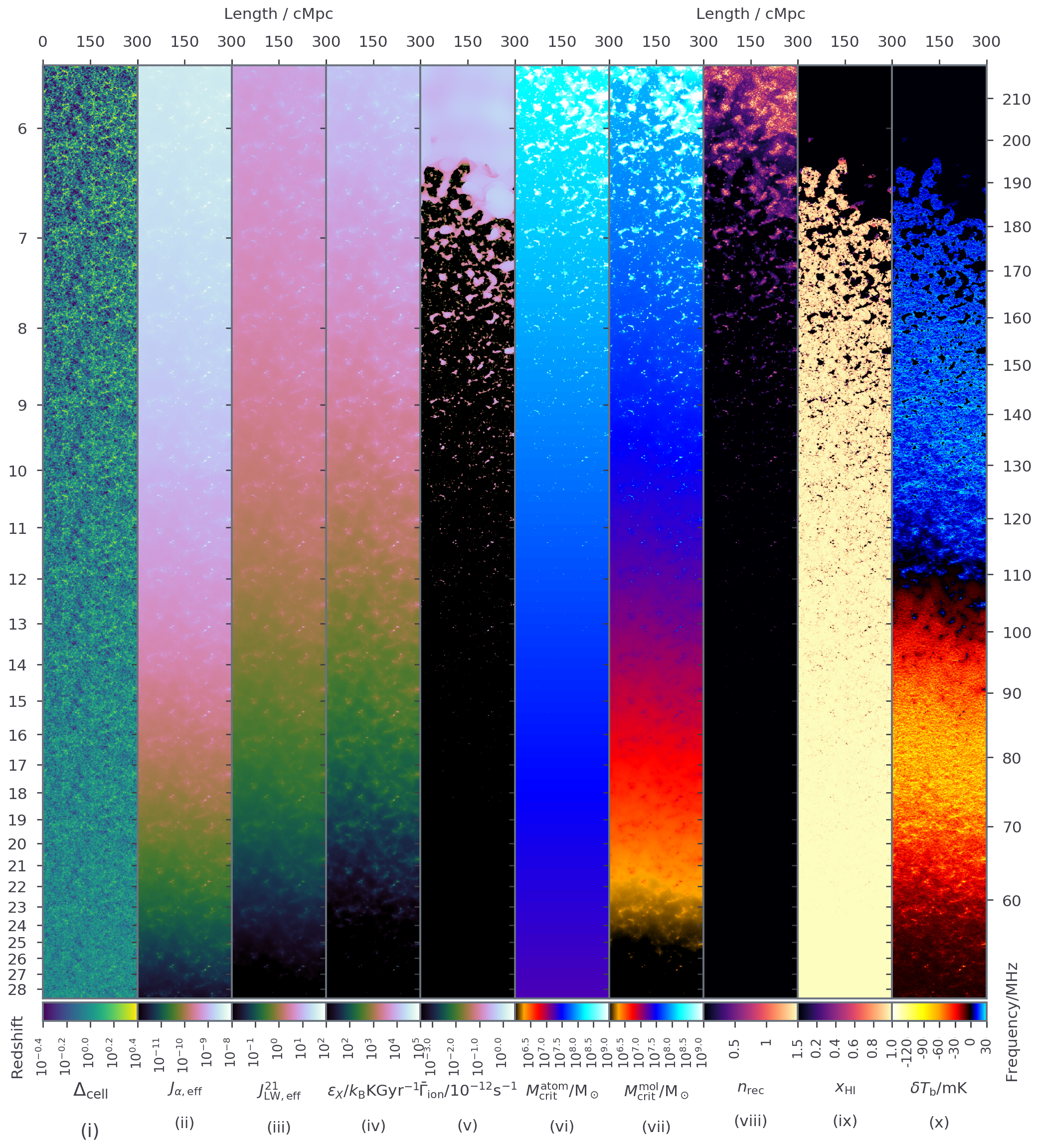
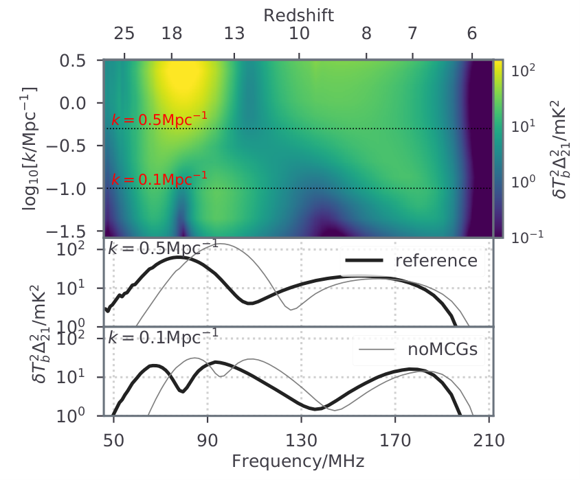
We summarize the relevant model parameters in Table 1 together with the values chosen for a reference model. We present this reference model, including slices through various fields in Fig. 3 and the 21-cm power spectra in Fig. 4. Simulations presented in this section share the same initial conditions and are performed within periodic boxes that have a comoving length of 300Mpc and a cell resolution of 1.17Mpc (300Mpc/256). Unless otherwise specified, values are consistent with those in 128, for the parameters the two works have in common. We will demonstrate below how current observations can constrain a subset of these parameters in Section 4.
Looking at the light-cones in Fig. 3, we see immediately that the structure of the 21-cm signal (rightmost panel) is governed by various radiation fields, with specific fields dominating at different epochs. The early 21-cm structures () are imprinted by the Lyman- background (second panel), which is fairly uniform. However, regions around the nascent galaxies, which are hosted by large-scale matter overdensities (first panel), see enhanced fluxes by factors of up to a few. These regions also have a higher LW flux (third panel), with intensities reaching values large enough for negative feedback on MCGs (seventh panel) during the Lyman- coupling epoch. By , the LW feedback is significant through the IGM – the median exceeds and the critical mass, , becomes more than three times the molecular-cooling threshold (see equation 11), leading to a factor of suppression on the number density of low-mass MCGs.
Shortly thereafter, X-rays from the first galaxies begin to dominate the thermal evolution of the IGM (fourth panel). By , exceeds in most parts of the simulation box, overcoming adiabatic cooling of the gas (see equation 14). With becoming positive, reaches its minimum and we see an absorption feature in the 21-cm light-cone, which fades away at (see also Fig. 4). After that, gas becomes hotter than the CMB and the signal is in emission.
(A high-resolution version of this figure is available at http://homepage.sns.it/mesinger/Media/light-cones_minihalo.png.)

| Parameter | Sec. | Eq. | Description | Ref. | MCMC |
| 2.1.1 | 2 | Stellar-to-halo mass ratio at for | -1.25 | -1.25 | |
| 2.1.2 | 8 | -1.75 | [-3, 0] | ||
| 2.1.1,2.1.2 | 2,8 | Stellar-to-halo mass power-law index | 0.5 | 0.5 | |
| 2.1.1 | 3 | Star formation time-scale in units of | 0.5 | 0.5 | |
| 2.1.1,2.1.2 | 5,10 | Critical halo mass for supernova feedbacka | - | - | |
| 2.1.1 | 12 | Self-shielding factor of for LW dissociation | 0.0 | 0.0 | |
| 2.3.1 | 16 | Number of ionizing photons emitted per stellar baryon for | |||
| 2.3.1 | 16 | ||||
| 2.3.1 | 17 | Escape fraction of ionizing photons at for | -1.22 | [-3, 0] | |
| -2.22 | [-3, 0] | ||||
| 2.3.1 | 17 | Escape fraction of ionizing photons to halo mass power-law indices for | 0 | 0 | |
| 0 | 0 | ||||
| 2.3.1 | 19 | Spectral index of the ionizing background | 5 | 5 | |
| 2.3.3 | 23 | Minimum X-ray energy escaping the galaxies into the IGM | 500 | [100, 1500] | |
| 2.3.3 | 23 | Spectral index of X-ray sourcesb | 1.0 | 1.0 | |
| 2.3.3 | 23 | Soft-band X-ray luminosity per SFR in units of for | 40.5 | [38,44]c | |
| 40.5 |
- a
Although it is a free parameter, for this work we maximize the importance of small galaxies by assuming supernova feedback is subdominant compared to inefficient cooling and photoheating in determining the faint turnover, i.e. ;
- b
In this work, we set , motivated by observations of (population-averaged) spectra of high-mass X-ray binaries in local galaxies (e.g. Mineo et al. 2012; Fragos et al. 2013; Pacucci et al. 2014).
- c
We assume that ACGs and MCGs possess similar X-ray luminosities during MCMC, i.e. .
The EoR (second to last panel), as well as the associated photoheating feedback (sixth panel) and recombinations fields (eight panel), is driven by short mean free path ionizing photons. Therefore, their evolution is not sensitive to a diffuse, increasing background (as is the case for X-rays and LW photons) but proceeds in a “percolating fashion” (e.g. Furlanetto & Oh 2016) with medium-to-large scales being closely tied to the underlying density field (e.g. Zahn et al. 2011; Battaglia et al. 2013; McQuinn & D’Aloisio 2018). The EoR history of this model is chosen to agree with current observational constraints, finishing by (e.g. McGreer et al. 2015), having a mid-point of around (Planck Collaboration et al. 2016a), and a small tail extending to higher redshifts corresponding to small HII regions around the nascent first galaxies (e.g. Mitra et al. 2015; Greig & Mesinger 2017).
The 21-cm PS of this model, presented in Fig. 4, shows the characteristic triple peak structure of the large-scale power evolution, driven by fluctuations in the Lyman- coupling, X-ray heating, and reionization fields. On smaller scales, the first two peaks merge due to a larger negative contribution of the cross-terms of the component fields (see discussions in Pritchard & Furlanetto 2007; Baek et al. 2010; Mesinger et al. 2013). For reference, we also show in grey the same astrophysical model but with no minihaloes. We see in general that the astrophysical epochs in this model are delayed, especially the earliest ones, and there is more power on large scales. We will return to this below.

3.2 Parameter dependence
Here we vary some of the astrophysical parameters characterizing MCGs, illustrating the resulting impact on cosmic fields. In Fig. 5, we show the redshift evolution of the median values of various fields in the top rows, together with the 21-cm PS in the bottom rows. Along the columns, we vary the normalization of the stellar-to-halo mass relation (i.e. ratio at ; ), the ionizing escape fraction (), the soft-band X-ray luminosity per SFR () and self-shielding factor of (). We only vary one parameter at a time, fixing the remaining parameters to those of the reference model. The general trends are the following:
- 1.
varying leads to different production rates of photons in all wavelengths of interest. An increasing stellar mass in MCGs shifts all astrophysical epochs to earlier times. Understandably, the earlier epochs of Lyman- pumping and X-ray heating are most affected, as MCGs have a larger relative contribution at higher redshifts. However increasing the efficiency to 10 times our fiducial one (or analogously increasing the ionizing escape fraction) shifts reionization to earlier times. In this case, MCGs can contribute more ionizing photons than ACGs well into the EoR (; comparing grey and red dotted curves in the fourth row), and the midpoint of the EoR shifts to ;
- 2.
varying around our fiducial model only has a minor impact on the timing of the EoR. Because the overall emission of ionizing photons depends on the product of the escape fraction and the SFR, increasing the escape fraction by a factor of 10 results in a shift of the EoR to earlier times, as seen in the previous column. Note that the stellar mass and the escape fraction do not have a completely degenerate impact on the EoR timing as the star formation time-scale evolves with redshift, and radiative feedback can regulate star formation;
- 3.
varying impacts almost exclusively the Epoch of Heating (EoH), as X-rays are inefficient at reionizing the Universe. Increasing the X-ray luminosity shifts the EoH to earlier times. As a result, the EoR and Lyman- pumping epochs increasingly overlap, which dramatically reduces the maximum contrast between the gas and CMB temperatures, and the corresponding minima in the global signal. Moreover, the resulting 21-cm power on small and medium scales is also reduced due to the increased negative contribution of the cross-correlation between the temperature and Lyman- coupling fields;1414 14 In other words, during Lyman- pumping, the regions close to galaxies have the strongest coupling, with their spin temperatures approaching the gas temperature () while most of the IGM has a spin temperature close to that of the CMB (). Thus regions close to galaxies appear as cold spots in the 21-cm signal during this early stage when the IGM is still colder than the CMB. However, if X-ray heating is more efficient, the gas surrounding the first galaxies can heat up before coupling is completed. In such a case of strong overlap of the EoH and epoch of Lyman- coupling, regions close to galaxies can be heated and coupled (), while those regions distant from galaxies are still cold but not coupled (). In this case most of the IGM can have spin temperatures that are closer to the CMB temperature, reducing the mean 21-cm signal and spatial fluctuations.
- 4.
varying changes how sensitive MCGs respond to negative feedback from the LWB (e.g. Schauer et al. 2015). As our reference model assumes no self-shielding, , here we only increase this parameter to 0.5 and 0.9. A larger decreases the effective LW radiation penetrating the ISM of the galaxies (second row), decreasing the impact of LW feedback. With a correspondingly higher contribution of MCGs when self-shielding is increased, astrophysical epochs are shifted earlier; however, the effect is extremely small, indicating that negative LW feedback in our model is not very important.
We also present a model (noMCGs) where contribution from minihaloes is excluded. Comparing with noMCGs, we see that, depending on the values used for the aforementioned parameters, MCGs can be the dominant source of radiation in the early universe, governing the global evolution of 21-cm signal, and altering its morphology. Therefore, 21-cm observables can be a powerful tool to probe the properties of first galaxies. In the next section, we will quantify how current high-redshift observations can jointly constrain the properties of MCGs and ACGs within a Bayesian analysis framework.
4 Inferring the astrophysics of minihaloes
The previous section illustrates how varying galaxy properties can impact the 21-cm signal. However, our model has many free parameters which characterize both ACGs and MCGs. Can these parameters be constrained by current and upcoming observations? In a companion paper, we will quantify the parameter constraints and degeneracies available with future 21-cm interferometric observations. Here we focus on current observations of the EoR and CD, seeing if these can already be used to inform our model and infer the astrophysics of minihaloes. These observations 1515 15 We assume the corresponding uncertainties to be Gaussian or one-sided Gaussian (for upper limits). include
- 1.
the galaxy UV LF at from Bouwens et al. 2015; Bouwens et al. 2016 and Oesch et al. 2018;
- 2.
the upper limit on the neutral hydrogen fraction at , , measured using the dark fraction of QSO spectra (McGreer et al. 2015);
- 3.
the Thomson scattering optical depth of CMB photons reported by Planck Collaboration et al. 2016a, ; and
- 4.
the timing1616 16 If the EDGES signal is indeed cosmological, its amplitude could only be explained with non-standard models (e.g. Ewall-Wice et al. 2018; Fialkov et al. 2018; Muñoz & Loeb 2018; Mebane et al. 2020). We do not go into the physical sources of the unexpectedly deep absorption signal in this work. Nevertheless, current explanations still rely on X-rays and soft UV radiation from galaxies to govern its timing. of the 21-cm global absorption feature reported by EDGES, which has a minimum at a frequency of 78MHz (Bowman et al. 2018).
To quantify parameter constraints implied by these observations, we use the MCMC module, 21CMMC (Greig & Mesinger 2015; Greig & Mesinger 2017; Greig & Mesinger 2018), which forward-models 21-cm light-cones using the EMCEE sampler (Goodman & Weare 2010; Foreman-Mackey et al. 2013). Unfortunately, varying all of the model parameters listed in Table 1 is computationally challenging, and would require high-performance computing resources. We defer a larger parameter space exploration to future work.
For this introductory work, we limit our parameter space. Specifically, we fix the stellar-to-halo mass relation of ACGs to the recovered median values in 128, as current LFs already provide reasonable constraints on these parameters. These include: (i)) the stellar-to-halo mass ratio at for ACGs, ; (ii) the power-law index of the ACG stellar-to-halo mass relation, ; and (iii) the star formation time-scale, . Fixing these values ensures that the modelled galaxy UV LFs are in agreement with high-redshift observations at the bright end (see also Fig. 1).

Additionally, we consider constant escape fractions for each population (i.e. ), ignore self-shielding of (i.e. ), and further assume ACGs and MCGs possess a similar X-ray luminosity per SFR1717 17 Although the X-ray luminosity of HMXBs scales with decreasing metallicity (Mapelli et al. 2010; Douna et al. 2015; Brorby et al. 2016), theoretically this trend is expected to saturate for metallicities below roughly 10 per cent solar (e.g. Fragos et al. 2013). Thus, assuming similar X-ray luminosity to SFRs for ACGs and MCGs could be reasonable if the level of metal enrichment in early ACGs is fairly modest. In any case, our results can be treated as a lower limit on the contribution of MCGs to the X-ray background. (i.e. ).
We thus explore the following parameters with flat priors in linear or logarithmic scale:
- 1.
the normalization of the MCG stellar-to-halo mass ratio, ;
- 2.
the escape fraction of ionizing photons for ACGs, ;
- 3.
the escape fraction of ionizing photons for MCGs, ;
- 4.
the minimum energy for X-rays to reach the IGM, ; and
- 5.
the soft-band X-ray luminosity per SFR, .
For the sake of computing efficiency, we have chosen a slightly smaller box with a comoving length of 250Mpc and a cell resolution of 1.95Mpc (250Mpc/128) when performing the MCMC.
Fig. 6 shows the marginalized posterior distributions together with the corresponding marginalized [14, 86] percentiles of the average EoR and 21-cm redshift evolutions. We also identify the timing when reaches its minimum as well as the full width at half-maximum (FWHM) of frequency, and show their PDFs in the right-hand subpanels. The red curves and shaded areas correspond to constraints using all of the above observations, except EDGES (noEDGES). Even without EDGES, we see a strong degeneracy between the allowed SFR and the ionizing escape fractions in MCGs – high values of either or are excluded, as they would reionize the Universe too early to be consistent with Planck observations (see also, e.g. Visbal et al. 2015). On the other hand, an escape fraction of ionizing photons in ACGs of % is required to ensure a sufficiently ionized universe at . As expected, without any information of 21cm, the X-ray properties cannot be constrained by any of these measurements.
We then add in the constraints from EDGES timing (EDGES_FREQ). The corresponding marginalized PDFs are shown with blue curves and shaded regions. Most constraints tighten only slightly when including the timing of the EDGES signal. In particular, the aforementioned degeneracy between the stellar-halo mass ratio and ionizing escape fraction is mostly unchanged. We fit this degeneracy in both cases to obtain the following relations (median with [14, 86] percentiles):
| (33) |
However, the most striking change is in the – plane. We see that a strong degeneracy emerges between these two parameters
| (34) |
If the EDGES signal at MHz is cosmological, soft UV and X-ray photons from galaxies are needed at 17–20 to source the Lyman- coupling and subsequent X-ray heating transitions, regardless of the physical explanation of the depth of the signal (Madau 2018; Mirocha & Furlanetto 2019). However, the stellar-to-halo mass relation implied by observations of high-redshift UV LFs is insufficient to heat the IGM at such high redshifts (Mirocha et al. 2016; Mirocha & Furlanetto 2019; Park et al. 2020). This is in contrast with early estimates of X-ray heating, based on assumptions of a constant stellar-to-halo mass ratio (e.g. Mesinger et al. 2016; Fialkov et al. 2018). As a result, the cosmological explanation of the EDGES signal requires MCGs to set the timing of the signal.1818 18 One could get around this claim if the ACGs were allowed to have higher values for the X-ray luminosity-to-SFR relation, i.e. . However, this is contrary to the expected trend, since for HMXBs should increase with decreasing metallicity (e.g. Mapelli et al. 2010; Douna et al. 2015; Brorby et al. 2016).
We quantify this claim further in Fig. 7, which shows the relative contribution of MCGs and ACGs in the LWB, Lyman- background, cumulative ionizing photon number, and X-ray heating rates, corresponding to the EDGES_FREQ posterior1919 19 The contribution of ACGs to and does not have a spread for our posterior, since we are fixing and (motivated by the comparably tight, dex constraints on these parameters from current LF observations; 128), and since we are assuming that SN feedback is subdominant in setting the turnover mass (which maximizes the abundances of ACGs). Varying the X-ray luminosity and escape fraction, however, does result in a spread in the X-ray heating and cumulative number of ionizing photos per baryon for ACGs.. We see that MCGs dominate the LW, Lyman-, UV ionizing and X-ray radiation at , , and , respectively, showing that they are the dominant population during the cosmological interpretation of the EDGES signal.
Nevertheless, we note that the MCGs required for explaining EDGES timing are still “unusual”. The degeneracies quantified in equations (33) and (34) mean that MCGs must have been inefficient at producing ionizing photons but efficient in emitting X-ray photons. For example, if the ionizing escape fraction of MCGs was above 10 percent (e.g. Xu et al. 2016), then in order to match both Planck and EDGES observations, the star formation (X-ray production) efficiencies of MCGs must have been a factor of 10 smaller (100-1000 greater) than those of ACGs. In Fig. 6, we indicate the expected range for if HMXBs were similar to those in local galaxies (Mineo et al. 2012) extrapolated to low-metallicity environments (Fragos et al. 2013). We see qualitatively that most MCGs require higher X-ray efficiencies than are theoretically expected even extrapolating to metal-free environments.
Finally, in Fig. 8, we show the marginalized UV LFs of ACGs2020 20 We see that, by fixing , ACG UV LFs only show large uncertainties at low redshifts and faint galaxies, when photoheating feedback from reionization becomes significant. As stated previously, this is due to our assumption of , so as to maximize the star formation in faint galaxies, which are the focus of this work. Thus, we caution that the scatter in the ACG LFs is underestimated. and MCGs corresponding to the EDGES_FREQ posterior (blue shaded regions; the noEDGES LFs are comparable due to the similar distributions of and between these two results). Comparing between LFs of MCGs and ACGs, we recover the result from Fig. 1 and find that MCGs likely only dominate at very high redshifts and faint magnitudes.
5 Conclusions
In this work, we include the first, molecularly cooled galaxies that are expected to start the CD in the public 21cmFAST simulation code. We consider atomic- (ACGs) and molecular-cooled galaxies (MCGs) as two different populations that source the underlying radiation backgrounds and drive the structure of 21-cm brightness temperature. We allow the stellar mass and SEDs of the two galaxy populations to scale differently with the host halo mass. We track inhomogeneous recombinations and self-consistently follow the relevant radiative feedback mechanisms, including inhomogeneous LW feedback and photoheating feedback on star formation.
We demonstrate how 21-cm observables vary with MCG properties. These include their star formation efficiencies, UV ionizing escape fractions, X-ray luminosities and self-shielding factors against LWB. We then use the Bayesian analysis tool, 21CMMC, to quantify what current observations imply for the MCG population. We use constraints from: (i) current galaxy luminosity functions at (Bouwens et al. 2015; Bouwens et al. 2016; Oesch et al. 2018); (ii) the dark fraction upper limit on the neutral hydrogen fraction at (McGreer et al. 2015); and (iii) the Thomson scattering optical depth of the CMB (Planck Collaboration et al. 2016a). We find that the optical depth already rules out models with a high stellar-to-halo mass ratio and high escape fractions in MCGs (Visbal et al. 2015).
We also consider the timing of the first claimed detection of the sky-average 21-cm brightness temperature, from EDGES, as an ancillary data set. We find that MCGs are required to produce a global absorption signal around 78MHz. Moreover, the resulting strong degeneracy between the SFRs and X-ray luminosities of MCGs implies that they would have unexpected properties. For example, if the ionizing escape fraction of MCGs was above 10 per cent (e.g. Xu et al. 2016), then in order to match both Planck and EDGES observations, the star formation (X-ray production) efficiencies of MCGs must have been a factor of 10 smaller (100-1000 greater) than those of ACGs. We conclude that the high-redshift 21-cm signal can be a powerful probe of the properties of the first galaxies, which are too faint to be studied using direct observations even with JWST.
Acknowledgements
The authors thank Zoltan Haiman and the anonymous referee for their comprehensive review and positive comments. This work was supported by the European Research Council (ERC) under the European Union’s Horizon 2020 research and innovation programme (AIDA – #638809). Parts of this research were supported by the Australian Research Council Centre of Excellence for All Sky Astrophysics in 3 Dimensions (ASTRO 3D), through project #CE170100013 as well as the NSF grant AST-1813694.
References
- Ahn et al. (2012) Ahn K., Iliev I. T., Shapiro P. R., Mellema G., Koda J., Mao Y., 2012, ApJ, 756, L16
- Ahn et al. (2009) Ahn K., Shapiro P. R., Iliev I. T., Mellema G., Pen U.-L., 2009, ApJ, 695, 1430
- Atek et al. (2018) Atek H., Richard J., Kneib J.-P., Schaerer D., 2018, MNRAS, 479, 5184
- Baek et al. (2010) Baek S., Semelin B., Di Matteo P., Revaz Y., Combes F., 2010, A&A, 523, A4
- Barkana & Loeb (2001) Barkana R., Loeb A., 2001, Physics Reports, 349, 125
- Barkana & Loeb (2005) Barkana R., Loeb A., 2005, ApJ, 626, 1
- Battaglia et al. (2013) Battaglia N., Trac H., Cen R., Loeb A., 2013, ApJ, 776, 81
- Beardsley et al. (2016) Beardsley A. P. et al., 2016, ApJ, 833, 102
- Behroozi et al. (2019) Behroozi P., Wechsler R. H., Hearin A. P., Conroy C., 2019, MNRAS, 488, 3143
- Bhatawdekar et al. (2019) Bhatawdekar R., Conselice C. J., Margalef-Bentabol B., Duncan K., 2019, MNRAS, 843
- Bouwens et al. (2015) Bouwens R. J. et al., 2015, ApJ, 803, 34
- Bouwens et al. (2017) Bouwens R. J., Oesch P. A., Illingworth G. D., Ellis R. S., Stefanon M., 2017, ApJ, 843, 129
- Bouwens et al. (2016) Bouwens R. J. et al., 2016, ApJ, 830, 67
- Bowman et al. (2018) Bowman J. D., Rogers A. E., Monsalve R. A., Mozdzen T. J., Mahesh N., 2018, Nature, 555, 67
- Bradley et al. (2019) Bradley R. F., Tauscher K., Rapetti D., Burns J. O., 2019, ApJ, 874, 153
- Bromm et al. (2001) Bromm V., Kudritzki R. P., Loeb A., 2001, ApJ, 552, 464
- Bromm & Larson (2004) Bromm V., Larson R. B., 2004, ARA&A, 42, 79
- Brorby et al. (2016) Brorby M., Kaaret P., Prestwich A., Mirabel I. F., 2016, MNRAS, 457, 4081
- Cen (2003) Cen R., 2003, ApJ, 591, 12
- Ciardi et al. (2006) Ciardi B., Scannapieco E., Stoehr F., Ferrara A., Iliev I. T., Shapiro P. R., 2006, MNRAS, 366, 689
- Dalal et al. (2010) Dalal N., Pen U.-L., Seljak U., 2010, JCAP, 1011, 007
- Dalla Vecchia & Schaye (2008) Dalla Vecchia C., Schaye J., 2008, MNRAS, 387, 1431
- Dalla Vecchia & Schaye (2012) Dalla Vecchia C., Schaye J., 2012, MNRAS, 426, 140
- Das et al. (2017) Das A., Mesinger A., Pallottini A., Ferrara A., Wise J. H., 2017, MNRAS, 469, 1166–1174
- Datta et al. (2014) Datta K. K., Jensen H., Majumdar S., Mellema G., Iliev I. T., Mao Y., Shapiro P. R., Ahn K., 2014, MNRAS, 442, 1491
- Datta et al. (2012) Datta K. K., Mellema G., Mao Y., Iliev I. T., Shapiro P. R., Ahn K., 2012, MNRAS, 424, 1877
- Dayal et al. (2014) Dayal P., Ferrara A., Dunlop J. S., Pacucci F., 2014, MNRAS, 445, 2545
- DeBoer et al. (2017) DeBoer D. R. et al., 2017, PASP, 129, 045001
- Dijkstra et al. (2004) Dijkstra M., Haiman Z., Rees M. J., Weinberg D. H., 2004, ApJ, 601, 666
- Douna et al. (2015) Douna V. M., Pellizza L. J., Mirabel I. F., Pedrosa S. E., 2015, A&A, 579, A44
- Draine & Bertoldi (1996) Draine B. T., Bertoldi F., 1996, ApJ, 468, 269
- Efstathiou (1992) Efstathiou G., 1992, MNRAS, 256, 43P
- Eldridge et al. (2017) Eldridge J. J., Stanway E. R., Xiao L., McClelland L. A. S., Taylor G., Ng M., Greis S. M. L., Bray J. C., 2017, PASA, 34, e058
- Evoli et al. (2014) Evoli C., Mesinger A., Ferrara A., 2014, J. Cosmology Astropart. Phys, 2014, 024
- Ewall-Wice et al. (2018) Ewall-Wice A., Chang T. C., Lazio J., Doré O., Seiffert M., Monsalve R. A., 2018, ApJ, 868, 63
- Ferrara & Loeb (2013) Ferrara A., Loeb A., 2013, MNRAS, 431, 2826
- Fialkov & Barkana (2014) Fialkov A., Barkana R., 2014, MNRAS, 445, 213
- Fialkov et al. (2018) Fialkov A., Barkana R., Cohen A., 2018, Physical Review Letters, 121, 011101
- Fialkov et al. (2012) Fialkov A., Barkana R., Tseliakhovich D., Hirata C. M., 2012, MNRAS, 424, 1335
- Fialkov et al. (2013) Fialkov A., Barkana R., Visbal E., Tseliakhovich D., Hirata C. M., 2013, MNRAS, 432, 2909
- Finkelstein (2016) Finkelstein S. L., 2016, PASA, 33, e037
- Finkelstein et al. (2015) Finkelstein S. L. et al., 2015, ApJ, 810, 71
- Foreman-Mackey et al. (2013) Foreman-Mackey D., Hogg D. W., Lang D., Goodman J., 2013, PASP, 125, 306
- Fragos et al. (2013) Fragos T. et al., 2013, ApJ, 764, 41
- Furlanetto & Furlanetto (2007) Furlanetto S. R., Furlanetto M. R., 2007, MNRAS, 374, 547
- Furlanetto & Oh (2016) Furlanetto S. R., Oh S. P., 2016, MNRAS, 457, 1813
- Furlanetto et al. (2006) Furlanetto S. R., Oh S. P., Briggs F. H., 2006, Phys. Rep., 433, 181
- Furlanetto & Stoever (2010) Furlanetto S. R., Stoever S. J., 2010, MNRAS, 404, 1869
- Furlanetto et al. (2004) Furlanetto S. R., Zaldarriaga M., Hernquist L., 2004, ApJ, 613, 1
- Garaldi et al. (2019) Garaldi E., Compostella M., Porciani C., 2019, MNRAS, 483, 5301
- Gardner et al. (2006) Gardner J. P. et al., 2006, Space Sci. Rev., 123, 485
- Goodman & Weare (2010) Goodman J., Weare J., 2010, Communications in Applied Mathematics and Computational Science, 5, 65
- Greif et al. (2011) Greif T. H., White S. D. M., Klessen R. S., Springel V., 2011, ApJ, 736, 147
- Greig & Mesinger (2015) Greig B., Mesinger A., 2015, MNRAS, 449, 4246
- Greig & Mesinger (2017) Greig B., Mesinger A., 2017, MNRAS, 472, 2651
- Greig & Mesinger (2017) Greig B., Mesinger A., 2017, MNRAS, 465, 4838
- Greig & Mesinger (2018) Greig B., Mesinger A., 2018, MNRAS, 477, 3217
- Haiman et al. (2000) Haiman Z., Abel T., Rees M. J., 2000, ApJ, 534, 11
- Haiman et al. (1996) Haiman Z., Rees M. J., Loeb A., 1996, ApJ, 467, 522
- Haiman et al. (1997) Haiman Z., Rees M. J., Loeb A., 1997, ApJ, 476, 458
- Hassan et al. (2016) Hassan S., Davé R., Finlator K., Santos M. G., 2016, MNRAS, 457, 1550
- Hektor et al. (2018) Hektor A., Hütsi G., Marzola L., Raidal M., Vaskonen V., Veermäe H., 2018, Phys. Rev. D, 98, 023503
- Hills et al. (2018) Hills R., Kulkarni G., Meerburg P. D., Puchwein E., 2018, Nature, 564, E32–E34
- Hirata (2006) Hirata C. M., 2006, MNRAS, 367, 259
- Holzbauer & Furlanetto (2012) Holzbauer L. N., Furlanetto S. R., 2012, MNRAS, 419, 718
- Hopkins et al. (2014) Hopkins P. F., Kereš D., Oñorbe J., Faucher-Giguère C.-A., Quataert E., Murray N., Bullock J. S., 2014, MNRAS, 445, 581
- Hopkins et al. (2018) Hopkins P. F. et al., 2018, MNRAS, 480, 800–863
- Hui & Gnedin (1997) Hui L., Gnedin N. Y., 1997, MNRAS, 292, 27
- Ishigaki et al. (2018) Ishigaki M., Kawamata R., Ouchi M., Oguri M., Shimasaku K., Ono Y., 2018, ApJ, 854, 73
- Jaacks et al. (2019) Jaacks J., Finkelstein S. L., Bromm V., 2019, MNRAS, 488, 2202–2221
- Jensen et al. (2013) Jensen H. et al., 2013, MNRAS, 435, 460
- Johnson et al. (2007) Johnson J. L., Greif T. H., Bromm V., 2007, ApJ, 665, 85
- Katz et al. (2020) Katz H. et al., 2020, MNRAS, 494, 2200–2220
- Keller et al. (2014) Keller B. W., Wadsley J., Benincasa S. M., Couchman H. M. P., 2014, MNRAS, 442, 3013
- Kimm & Cen (2014) Kimm T., Cen R., 2014, ApJ, 788, 121
- Kimm et al. (2017) Kimm T., Katz H., Haehnelt M., Rosdahl J., Devriendt J., Slyz A., 2017, MNRAS, stx052
- Koh & Wise (2018) Koh D., Wise J. H., 2018, MNRAS, 474, 3817
- Kohn et al. (2019) Kohn S. A. et al., 2019, ApJ, 882, 58
- Koopmans et al. (2015) Koopmans L. V. E. et al., 2015
- Kuhlen & Faucher-Giguère (2012) Kuhlen M., Faucher-Giguère C.-A., 2012, MNRAS, 423, 862
- Leitherer et al. (1999) Leitherer C. et al., 1999, ApJS, 123, 3
- Lippai et al. (2009) Lippai Z., Frei Z., Haiman Z., 2009, ApJ, 701, 360
- Liu et al. (2016) Liu C., Mutch S. J., Angel P. W., Duffy A. R., Geil P. M., Poole G. B., Mesinger A., Wyithe J. S. B., 2016, MNRAS, 462, 235
- Livermore et al. (2017) Livermore R. C., Finkelstein S. L., Lotz J. M., 2017, ApJ, 835, 113
- Lopez-Honorez et al. (2016) Lopez-Honorez L., Mena O., Moliné Á., Palomares-Ruiz S., Vincent A. C., 2016, J. Cosmology Astropart. Phys, 2016, 004
- Ma et al. (2018) Ma X. et al., 2018, MNRAS, 478, 1694
- Ma et al. (2015) Ma X., Kasen D., Hopkins P. F., Faucher-Giguère C.-A., Quataert E., Kereš D., Murray N., 2015, MNRAS, 453, 960
- Madau (2018) Madau P., 2018, Monthly Notices of the Royal Astronomical Society: Letters, 480, L43–L47
- Madau & Dickinson (2014) Madau P., Dickinson M., 2014, Annual Review of Astronomy and Astrophysics, 52, 415
- Manti et al. (2017) Manti S., Gallerani S., Ferrara A., Greig B., Feruglio C., 2017, MNRAS, 466, 1160
- Mao et al. (2012) Mao Y., Shapiro P. R., Mellema G., Iliev I. T., Koda J., Ahn K., 2012, MNRAS, 422, 926
- Mapelli et al. (2010) Mapelli M., Ripamonti E., Zampieri L., Colpi M., Bressan A., 2010, MNRAS, 408, 234
- Mason et al. (2015) Mason C. A., Trenti M., Treu T., 2015, ApJ, 813, 21
- McGreer et al. (2015) McGreer I. D., Mesinger A., D’Odorico V., 2015, MNRAS, 447, 499
- McQuinn & D’Aloisio (2018) McQuinn M., D’Aloisio A., 2018, Journal of Cosmology and Astroparticle Physics, 2018, 016–016
- McQuinn et al. (2007) McQuinn M., Lidz A., Zahn O., Dutta S., Hernquist L., Zaldarriaga M., 2007, MNRAS, 377, 1043
- McQuinn & O’Leary (2012) McQuinn M., O’Leary R. M., 2012, ApJ, 760, 3
- Mebane et al. (2020) Mebane R. H., Mirocha J., Furlanetto S. R., 2020, MNRAS, 493, 1217–1226
- Mellema et al. (2013) Mellema G. et al., 2013, Experimental Astronomy, 36, 235
- Mesinger & Dijkstra (2008) Mesinger A., Dijkstra M., 2008, MNRAS, 390, 1071
- Mesinger et al. (2013) Mesinger A., Ferrara A., Spiegel D. S., 2013, MNRAS, 431, 621
- Mesinger & Furlanetto (2007) Mesinger A., Furlanetto S., 2007, ApJ, 669, 663
- Mesinger et al. (2011) Mesinger A., Furlanetto S., Cen R., 2011, MNRAS, 411, 955
- Mesinger et al. (2016) Mesinger A., Greig B., Sobacchi E., 2016, MNRAS, 459, 2342
- Mesinger et al. (2012) Mesinger A., McQuinn M., Spergel D. N., 2012, MNRAS, 422, 1403
- Miller et al. (2015) Miller B. P., Gallo E., Greene J. E., Kelly B. C., Treu T., Woo J.-H., Baldassare V., 2015, ApJ, 799, 98
- Mineo et al. (2012) Mineo S., Gilfanov M., Sunyaev R., 2012, MNRAS, 419, 2095
- Miralda-Escudé et al. (2000) Miralda-Escudé J., Haehnelt M., Rees M. J., 2000, ApJ, 530, 1
- Miranda et al. (2017) Miranda V., Lidz A., Heinrich C. H., Hu W., 2017, MNRAS, 467, 4050
- Mirocha & Furlanetto (2019) Mirocha J., Furlanetto S. R., 2019, MNRAS, 483, 1980
- Mirocha et al. (2016) Mirocha J., Furlanetto S. R., Sun G., 2016, MNRAS, 464, 1365–1379
- Mirocha et al. (2018) Mirocha J., Mebane R. H., Furlanetto S. R., Singal K., Trinh D., 2018, MNRAS, 478, 5591–5606
- Mitra et al. (2015) Mitra S., Roy Choudhury T., Ferrara A., 2015, Monthly Notices of the Royal Astronomical Society: Letters, 454, L76
- Moster et al. (2013) Moster B. P., Naab T., White S. D. M., 2013, MNRAS, 428, 3121
- Muñoz (2019a) Muñoz J. B., 2019a, Phys. Rev. D, 100, 063538
- Muñoz (2019b) Muñoz J. B., 2019b, Phys. Rev. Lett., 123, 131301
- Muñoz & Loeb (2018) Muñoz J. B., Loeb A., 2018, Nature, 557, 684
- Mutch et al. (2016) Mutch S. J., Geil P. M., Poole G. B., Angel P. W., Duffy A. R., Mesinger A., Wyithe J. S. B., 2016, MNRAS, 462, 250
- Naidu et al. (2020) Naidu R. P., Tacchella S., Mason C. A., Bose S., Oesch P. A., Conroy C., 2020, ApJ, 892, 109
- Noh & McQuinn (2014) Noh Y., McQuinn M., 2014, MNRAS, 444, 503
- Ocvirk et al. (2018) Ocvirk P. et al., 2018, arXiv e-prints, arXiv:1811.11192
- Oesch et al. (2018) Oesch P. A., Bouwens R. J., Illingworth G. D., Labbé I., Stefanon M., 2018, ApJ, 855, 105
- O’Leary & McQuinn (2012) O’Leary R. M., McQuinn M., 2012, ApJ, 760, 4
- O’Shea et al. (2015) O’Shea B. W., Wise J. H., Xu H., Norman M. L., 2015, ApJ, 807, L12
- Paardekooper et al. (2015) Paardekooper J.-P., Khochfar S., Dalla Vecchia C., 2015, MNRAS, 451, 2544
- Pacucci et al. (2014) Pacucci F., Mesinger A., Mineo S., Ferrara A., 2014, MNRAS, 443, 678–686
- Park et al. (2020) Park J., Gillet N., Mesinger A., Greig B., 2020, MNRAS, 491, 3891
- Park et al. (2019) Park J., Mesinger A., Greig B., Gillet N., 2019, MNRAS, 484, 933
- Parsa et al. (2017) Parsa S., Dunlop J. S., McLure R. J., 2017, MNRAS, 474, 2904–2923
- Patil et al. (2017) Patil A. H. et al., 2017, ApJ, 838, 65
- Planck Collaboration et al. (2016a) Planck Collaboration et al., 2016a, A&A, 596, A108
- Planck Collaboration et al. (2016b) Planck Collaboration et al., 2016b, A&A, 594, A13
- Pritchard & Furlanetto (2007) Pritchard J. R., Furlanetto S. R., 2007, MNRAS, 376, 1680
- Qin et al. (2019) Qin Y., Duffy A. R., Mutch S. J., Poole G. B., Mesinger A., Wyithe J. S. B., 2019, MNRAS, 487, 1946–1963
- Qin et al. (2017) Qin Y. et al., 2017, MNRAS, 472, 2009–2027
- Rahmati et al. (2013) Rahmati A., Pawlik A. H., Raičević M., Schaye J., 2013, MNRAS, 430, 2427
- Ricci et al. (2017) Ricci F., Marchesi S., Shankar F., La Franca F., Civano F., 2017, MNRAS, 465, 1915
- Ricotti et al. (2001) Ricotti M., Gnedin N. Y., Shull J. M., 2001, ApJ, 560, 580
- Ricotti & Ostriker (2004) Ricotti M., Ostriker J. P., 2004, MNRAS, 352, 547
- Sanderbeck et al. (2018) Sanderbeck P. R. U., McQuinn M., D’Aloisio A., Werk J. K., 2018, ApJ, 869, 159
- Schaerer (2002) Schaerer D., 2002, A&A, 382, 28
- Schauer et al. (2019) Schauer A. T. P., Glover S. C. O., Klessen R. S., Ceverino D., 2019, MNRAS, 484, 3510
- Schauer et al. (2015) Schauer A. T. P., Whalen D. J., Glover S. C. O., Klessen R. S., 2015, MNRAS, 454, 2441
- Scoccimarro (1998) Scoccimarro R., 1998, MNRAS, 299, 1097
- Seager et al. (1999) Seager S., Sasselov D. D., Scott D., 1999, ApJ, 523, L1
- Shang et al. (2010) Shang C., Bryan G. L., Haiman Z., 2010, MNRAS, 402, 1249
- Shapiro et al. (1994) Shapiro P. R., Giroux M. L., Babul A., 1994, ApJ, 427, 25
- Sims & Pober (2019) Sims P. H., Pober J. C., 2019, MNRAS, 488, 2904
- Sobacchi & Mesinger (2014) Sobacchi E., Mesinger A., 2014, MNRAS, 440, 1662
- Sun & Furlanetto (2016) Sun G., Furlanetto S. R., 2016, MNRAS, 460, 417
- Tacchella et al. (2018) Tacchella S., Bose S., Conroy C., Eisenstein D. J., Johnson B. D., 2018, ApJ, 868, 92
- Thoul & Weinberg (1996) Thoul A. A., Weinberg D. H., 1996, ApJ, 465, 608
- Tingay et al. (2013) Tingay S. J. et al., 2013, PASA, 30
- Trac & Gnedin (2011) Trac H. Y., Gnedin N. Y., 2011, Advanced Science Letters, 4, 228
- Tseliakhovich & Hirata (2010) Tseliakhovich D., Hirata C., 2010, Phys. Rev. D, 82, 083520
- Tumlinson & Shull (2000) Tumlinson J., Shull J. M., 2000, ApJ, 528, L65
- van Haarlem et al. (2013) van Haarlem M. P. et al., 2013, A&A, 556, A2
- Visbal et al. (2015) Visbal E., Haiman Z., Bryan G. L., 2015, MNRAS, 453, 4456
- Wilkins et al. (2019) Wilkins S. M., Lovell C. C., Stanway E. R., 2019, MNRAS, 490, 5359–5365
- Wise & Abel (2007) Wise J. H., Abel T., 2007, ApJ, 671, 1559
- Wise et al. (2012) Wise J. H., Turk M. J., Norman M. L., Abel T., 2012, ApJ, 745, 50
- Wolcott-Green et al. (2011) Wolcott-Green J., Haiman Z., Bryan G. L., 2011, MNRAS, 418, 838
- Wouthuysen (1952) Wouthuysen S. A., 1952, AJ, 57, 31
- Wyithe & Loeb (2013) Wyithe J. S. B., Loeb A., 2013, MNRAS, 428, 2741
- Xu et al. (2016) Xu H., Wise J. H., Norman M. L., Ahn K., O’Shea B. W., 2016, ApJ, 833, 84
- Yoshida et al. (2006) Yoshida N., Omukai K., Hernquist L., Abel T., 2006, ApJ, 652, 6
- Yoshida et al. (2003) Yoshida N., Sokasian A., Hernquist L., Springel V., 2003, ApJ, 598, 73
- Yung et al. (2019) Yung L. Y. A., Somerville R. S., Popping G., Finkelstein S. L., Ferguson H. C., Davé R., 2019, MNRAS, 490, 2855
- Zahn et al. (2011) Zahn O., Mesinger A., McQuinn M., Trac H., Cen R., Hernquist L. E., 2011, MNRAS, 414, 727
- Zygelman (2005) Zygelman B., 2005, ApJ, 622, 1356