Extended matter bounce scenario in ghost free gravity compatible with GW170817
Abstract
In the context of a ghost free model, an extended matter bounce scenario is studied where the form of the scale factor is given by . The ghost free character of the model is ensured by the presence of a Lagrange multiplier, as developed in Nojiri:2018ouv. The conditions under which, in this model, the speed of gravitational waves becomes equal to the speed of light (equal to one, in natural units), thus becoming compatible with the striking event GW170817, is investigated. It is shown that this happens for a class of Gauss-Bonnet (GB) coupling functions () which satisfies a constraint equation of the form , with the Hubble parameter. This constraint is then imposed on the ghost free gravity theory to be consistent with the GW170817 event, subsequently, the corresponding non-singular bouncing cosmology with the aforementioned scale factor is extensively studied. The forms of the coupling function and Lagrange multiplier in the “low curvature limit” of the theory are reconstructed, yielding a viable approximation for . Correspondingly, by solving the cosmological perturbation equation, the main observable quantities, namely the spectral index, tensor to scalar ratio, and the running index are determined and confronted with the latest Planck 2018 data. Consistency with the data is proven for those parametric regimes that which correspond to . This makes the low curvature approximation a viable one for calculating the scalar and tensor power spectra.
I Introduction
A major issue in theoretical cosmology is to ascertain whether the Universe was created from an initial singular or if, on the contrary, the Universe initiated its expansion from a non-singular, bounce-like stage. In other words, if the Universe evolved according to the standard cosmology evolution, for which the Universe emerges from an initial spacelike singularity, or if, in accordance with the bouncing theory, the Universe started its expansion with a non-zero value of the scalae factor. The inflationary picture guth; Linde:2005ht; Langlois:2004de; Riotto:2002yw; nb1; barrow1; barrow2; Banerjee:2017lxi; Chakraborty:2018scm; Elizalde:2018now; Elizalde:2018rmz; Nojiri:2019dwl has earned a lot of support, since it is able to resolve the horizon and flatness problems, and also generate an almost scale invariant power spectrum which is perfectly consistent with the observational data. However even the most recent observations could not yet undoubtedly confirm that inflation indeed took place, a direct proof of this fact (as would be, e.g., the direct or indirect detection of associated primordial gravitational waves) is still missing.
One of the alternative theories different from inflation is the bouncing scenario Brandenberger:2012zb; Brandenberger:2016vhg; Battefeld:2014uga; Novello:2008ra; Cai:2014bea; deHaro:2015wda; Nojiri:2019lqw; Lehners:2011kr; Lehners:2008vx; Cheung:2016wik; Cai:2016hea; Cattoen:2005dx; Li:2014era; Brizuela:2009nk; Cai:2013kja; Quintin:2014oea; Cai:2013vm; Poplawski:2011jz; Koehn:2015vvy; Odintsov:2015zza; Nojiri:2016ygo; Oikonomou:2015qha; Odintsov:2015ynk; Koehn:2013upa; Battarra:2014kga; Martin:2001ue; Khoury:2001wf; Buchbinder:2007ad; Brown:2004cs; Hackworth:2004xb; Nojiri:2006ww; Johnson:2011aa; Peter:2002cn; Gasperini:2003pb; Creminelli:2004jg; Lehners:2015mra; Mielczarek:2010ga; Lehners:2013cka; Cai:2014xxa; Cai:2007qw; Cai:2010zma; Avelino:2012ue; Barrow:2004ad; Haro:2015zda; Elizalde:2014uba; Das:2017jrl. This theory is also able to generate a nearly scale invariant power spectrum, thus becoming compatible with the observational data available. Moreover, a definite advantage of the bouncing scenario is that it avoids any spacetime singularity. In fact, the Big-Bang singularity could just be a manifestation of the shortcomings of classical gravity, which is certainly unable to describe the physical evolution at such small scales. Quite possibly, a yet-to-be-built quantum theory of gravity might be able to resolve the Big Bang singularity, as turned out to be actually the case in classical electrodynamics, with the Coulomb potential singularities at the origin of the potential, which are resolved in the context of quantum electrodynamics. However, in the absence of a fully accepted quantum gravity theory, the bouncing scenario reveals as a most promising theory to deal with this issue.
Among the various bouncing models proposed so far, the matter bounce scenario (MBS) deHaro:2015wda; Cai:2008qw; Finelli:2001sr; Quintin:2014oea; Cai:2011ci; Haro:2015zta; Cai:2011zx; Cai:2013kja; Haro:2014wha; Brandenberger:2009yt; deHaro:2014kxa; Odintsov:2014gea; Qiu:2010ch; Oikonomou:2014jua; Bamba:2012ka; deHaro:2012xj; WilsonEwing:2012pu has attracted a lot of attention, since it produces a nearly scale invariant power spectrum. In the matter bounce theory, the Universe evolved from an epoch at large negative time in the contracting era where the primordial spacetime perturbations are generated deeply inside the Hubble radius, and is thus able to solve the horizon problem. After bouncing, the Universe starts to expand with an evolution that is symmetric to the contraction phase. Here, it may be mentioned that another popular bounce scenario is the Big-Bounce one, which is also able to give a nearly scale invariant power spectrum. However in this last scenario, the perturbations are produced near the bouncing point, unlike what happens in the matter bounce model, where the perturbations originate, as mentioned earlier, deeply in the contracting phase. This is the scenario we will consider in the present paper, in particular the extended matter bounce scenario about which we will discuss later.
Despite the mentioned successes, the MBS still faces some problems, firstly, in an exact MBS characterized by a single scalar field, the power spectrum turns out to be exactly scale invariant (i.e the spectral index of the curvature perturbation is exactly equal to one), what does not match the observational constraints. Such inconsistency was also confirmed in Odintsov:2014gea from a slightly different viewpoint, namely from an gravity theory. It turns out that models can be equivalently mapped to scalar-tensor ones via conformal transformation of the metric Das:2017htt; Elizalde:2018rmz; Elizalde:2018now and, thus, the inconsistencies of the spectral index in the two different models are well justified. Secondly, according to the Planck 2018 data, the running of the spectral index is constrained to be . However, for the MBS in the case of a single scalar field model, the running of the index becomes zero and hence it is not compatible with observations. A zero running index is a consequence of the first problem. If the spectral index becomes exactly scale invariant, then the variation of the spectral index with respect to the mode momentum, i.e the running index, will obviously vanish. Thirdly, in the simplest MBS model, the amplitude of scalar fluctuations is found to be comparable to that of tensor perturbations, which in turn makes the value of the tensor-to-scalar ratio to be of order one, again in conflict with the Planck constraints. Lastly, the null energy condition in most of the bouncing models is violated when the bouncing is realized.
In order to solve all these issues, theories of modified gravity Nojiri:2010wj; Nojiri:2017ncd have been added to the picture, with success in many of the cases. For instance, in the so-called quasi-matter bounce scenario (which improves the exact matter bounce one), according to which the scale factor of the Universe evolves as (with ), deeply into the contracting era, it is possible to recover the consistency of the spectral index and of the running index, even in a single scalar field model deHaro:2015wda. However, the tensor-to-scalar ratio still remains a problem. From a different perspective, it has recently been shown Nojiri:2019lqw that an gravity model with Lagrange multiplier is able to resolve most of the problems arising in the context of matter or quasi-matter bounce scenarios, albeit it fails to restore the energy conditions. In such Lagrange multiplier gravity model, the tensor power spectrum becomes smaller in comparison with that of scalar perturbation and thus the tensor to scalar ratio lies within Planck constraints, unlike in pure gravity, where the observable parameters are not simultaneously compatible with the observational constraints.
The recently observed striking event of neutron star merging GW170817 GBM:2017lvd, reflects the fact that the propagation speed of the gravitational and electromagnetic waves are the same, i.e. equal to one in natural units. This observation has definitely narrowed down the viability of the modified gravitational theories, since every theory that predicts a gravitational wave speed different from one is no more a viable description (see Ref.[Ezquiaga:2017ekz] for a list of theories that are ruled out by GBM:2017lvd).
Motivated by the above arguments, we will here study an extended matter bounce scenario in the context of a ghost free model, as developed in Nojiri:2018ouv, and the conditions for such model to have gravitational waves speed () equal to one and thus become consistent with GW170817. As it was demonstrated in Nojiri:2018ouv, the constraint restricts the form of the Gauss-Bonnet coupling function. After finding the suitable form which also realizes the considered bounce model, we address the bouncing phenomenology of the resulting theory.
The paper is organized as follows. In Sect.[II], we briefly discuss the essential features of the ghost free model compatible with the event GW170817. Sections [III] and [IV] are respectively devoted to an extensive study of the primordial scalar and tensor perturbations and the observable parameters. Finally, the conclusions and remarks follow in the end of the paper.
II Essential features of a ghost-free gravity compatible with the GW170817 event
In this section we shall recall the essential features of the ghost free gravity theory developed in Ref. Nojiri:2018ouv. We consider which, owing to the presence of , contains ghosts with respect to perturbations of the spacetime metric. However the ghost modes may be eliminated by introducing a Lagrange multiplier in the standard gravity action Nojiri:2018ouv, leading to a ghost-free action, as follows
| (1) |
where is a constant with mass dimension [+1]. Upon variation with respect to the Lagrange multiplier , one obtains the following constraint equation
| (2) |
Effectively, the kinetic term is a constant, so it can be absorbed in the scalar potential, as
| (3) |
and the action of Eq. (1) can be rewritten as
| (4) |
The scalar and gravitational equations of motion for the action (4) take the form
| (5) | ||||
| (6) |
where has the following form,
with having in mind . Upon multiplication of Eq. (6) with , we get
| (7) |
and solving Eq. (7) with respect to yields
| (8) |
Eventually, we will deal with non-singular bounce cosmology in this ghost free model and, thus, the spatially flat Friedmann-Robertson-Walker (FRW) metric ansatz will fulfill our purpose. Let us now see how the equations of motion become if the metric background is a flat FRW one, with line element
| (9) |
Assuming that the functions and are only cosmic time dependent, and also that no matter fluids are present, that is, that , then Eq. (2) admits the following simple solution
| (10) |
Hence, the and components of Eq. (6) can be written as
| (11) | ||||
| (12) |
and, in addition, from Eq. (5) we get
| (13) |
By solving Eq. (11) with respect to , we obtain
| (14) |
It is easy to see that, by combining Eqs. (14) and (13), we obtain Eq. (12). Also by solving Eq. (12) with respect to the scalar potential , we get
| (15) |
Hence, for an arbitrarily chosen function , and with the potential being equal to
| (16) |
then we can realize an arbitrary cosmology corresponding to a given Hubble rate . Finally, the functional form of the Lagrange multiplier reads
| (17) |
As mentioned in the introductory section, here we are interested
on bouncing scenario followed from the theory with Lagrangian
(4). The cosmological perturbation, in particular the
tensor perturbation caused by the quantum vacuum fluctuation,
indicates the gravitational wave. On other hand, recently the
event GW170817 confirms the detection of the gravitational wave
which may has a different source than the quantum vacuum
fluctuation, and ensures that the speed of the gravitational wave
is equal to the speed of light (in natural units, it is equal to
unity). In the current paper, we consider that all the
gravitational waves generated from different sources (i.e from
black hole merging or from quantum vacuum fluctuations) have same
propagation speed, and due to GW170817, the speed is equal to
unity. With this consideration, we apply the result of GW170817 in
the present context of bouncing scenario. Earlier, the
implications of GW170817 on non-singular bounce has been
investigated, but in a different context i.e from a degenerate
higher order scalar-tensor (DHOST) theory Ye:2019frg,
unlike to the present paper where we discuss the bouncing scenario
from ghost free gravity model taking the
constraint of GW170817 into account.
The resulting theory with
Lagrangian (4) is a form of the scalar
Einstein-Gauss-Bonnet gravity along with a Lagrange multiplier,
for which it is well known that the speed of gravitational waves
is different from one, in particular, the gravitational wave speed
in the present context can be expressed as
Hwang:2005hb; Noh:2001ia; Hwang:2002fp,
| (18) |
with being the Hubble parameter. Eq.(18) apparently reflects the non-viability of the model with respect to GW170817 (which validates the fact that the gravitational and electromagnetic waves have the same propagation speed). However the gravitational wave speed in the ghost free model becomes one if the coupling function satisfies the following constraint equation Odintsov:2019clh,
| (19) |
Thereby, in order to make compatible our present model with GW170817, we consider such Gauss-Bonnet coupling functions which obey Eq.(19). Thus, a form of the Hubble parameter (later, we will consider the Hubble parameter in such a way that it gives an extended scenario of matter bounce cosmology) fixes in turn the coupling function via Eq.(19). At this stage it is worth mentioning that the new constraint on also fits with the original equations of motion, this being clear from the fact that there are two independent equations, namely the component of the gravitational equation and the equation for , and yet two unknown functions ((t), ) to determine. In the later section, we will consider a Hubble parameter which leads to an an extended matter bounce cosmology. In this context, it is worth mentioning that the presence of the potential term in model to realize a non-singular bounce cosmology which is also consistent with . Let us demonstrate this in more detail by examining the equations of motion without the potential term. For , eqn.(12) takes the following form-
| (20) |
Recall from eqn.(19), the Gauss-Bonnet coupling satisfies a constraint equation in order to make the propagation speed of the gravitational wave unity. On applying this constraint in eqn.(20), we get,
| (21) |
which immediately leads to the solution as - , OR . The first
possibility leads to the evolution of the scale factor as i.e an eternal matter dominated universe, On other hand, the second
possibility gives which along with the constraint makes the scale factor evolution as
i.e a Milne universe. Thus eqn.(21) is unable to realize a non-singular bounce cosmology. This indicates that
in absence of potential, model can not realize a non-singular bounce cosmology which is also consistent with
. However, in the present paper, as mentioned earlier, we will explore a non-singular bounce scenario in
model compatible with GW170817 and thus the consideration of the potential term becomes obvious from its own right.
In the next section, we shall extensively discuss the bouncing scenario of this model, which is both ghost free and
compatible with the GW170817 event.
III Realization of the extended matter bounce scenario
In this section we will discover which functional forms for and can realize a bouncing Universe cosmological scenario with the following scale factor
| (22) |
where and are the free parameters of the model,
having mass dimension [+2], while is dimensionless. The above
scale factor leads to a matter like bouncing universe. Here it may
be mentioned that the scale factor in eqn.(22) is
not the unique bouncing model that our universe may realize. There
are other possibilities of bounce, as for example - (1) the
exponential bouncing model where the scale factor evolves as and the bounce occurs at , (2) the
singular bounce scenario where the scale facor has the form
Odintsov:2015ynk. In the case of singular bounce, the
perturbation mode(s) generate near the time of
bouncing unlike to the usual bouncing model where the primordial perturbations generate in the past contracting phase deep inside the Hubble radius.
However, as mentioned in the introductory section, the matter-like bounce scenario demonstrated by the scale factor in eqn.(22),
faces some questions regarding the observational compatibility with Planck constraints, the instability of linear
order perturbation theory in super horizon scale etc. Motivated by such questions, we investigate the matter-like bounce scenario
in a modified gravity theory like model. Thus the calculations in the following sections of the paper are
based on this choice of the extended matter bounce scale factor. In this sense, one may argue that the results we will obtain depend on the ansatz
of the scale factor shown in eqn.(22).
The Universe’s evolution in a general bouncing cosmology, consists of
two eras, an era of contraction and an era of expansion. The above
scale factor describes a contracting era for the Universe, when
, then the Universe reaches a bouncing point, at
, at which the Universe has a minimal size, and then the
Universe starts to expand again, for cosmic times . Hence,
the Universe in this scenario never develops a crushing type Big
Bang singularity. It may be mentioned that for , the scale
factor describes a matter bounce scenario. Eq. (22) leads to the following Hubble rate and its first
derivative
| (23) |
With the help of the above expressions, the Ricci scalar is found to be,
| (24) |
Using Eq. (24), one can determine the cosmic time as a function of the Ricci scalar, that is the function . As a result, the Hubble rate and its first derivative can be expressed in terms of (this statement holds true for all analytic functions of ) and, also, the differential operator can be written as . However, for the purpose of determining as well as the observable quantities, we will consider the low curvature limit of the theory. Before proceeding further, let us comment on the viability of this approximation. We do it in the context of matter bounce cosmology, which is obtained by taking in Eq. (22), the primordial perturbations of the comoving curvature, which originate from quantum vacuum fluctuations. At subhorizon scales during the contracting era in the low-curvature regime, their wavelength was much smaller than the comoving Hubble radius, which is defined by . In the matter bounce evolution, the Hubble horizon radius decreases in size, and this causes the perturbation modes to exit from the horizon, eventually, with this exit occurring when the contracting Hubble horizon becomes equal to the wavelength of these primordial modes. However, in the present context, we consider a larger class of bouncing models of the form , always within Lagrange multiplier ghost free Gauss-Bonnet gravity. Thus, it will be important to check what are the possible values of which make the low-curvature limit, that is, a viable approximation in calculating the power spectrum for the bouncing model . This expression of the scale factor immediately leads to the comoving Hubble radius
| (25) |
Thereby diverges at , as expected because the
Hubble rate goes to zero at the bouncing point. Furthermore,
the asymptotic behavior of is given by ,
thus diverges for ,
otherwise goes to zero asymptotically. Hence, for ,
the comoving Hubble radius decreases initially in the contracting
era and then diverges near the bouncing point; unlike in the case
, where the Hubble radius increases from past infinity
and gradually diverges at . As a result, the possible range
of which leads the perturbation modes to exit the horizon at
large negative time and make the low-curvature limit a viable
approximation in calculating the power spectrum, is given by , see Fig[1], where it is shown that for , the perturbation modes can generate inside the Hubble horizon
at a large negative time.
Moreover, we will show in the later sections that this range of makes the observable quantities compatible
with the Planck constraints and, thus, the “low curvature limit” comes as a viable approximation to calculate the power spectra of scalar and tensor
perturbations.

In Fig[1], we show the spacetime sketch of our non-singular bouncing cosmology where the bounce time is taken at . We also plot the evolution of the physical length corresponding to a fixed co-moving scale. This scale is the wavelength of the fluctuation mode , with standing for the co-moving wavenumber. The wavelength begins at large negative time in the contracting phase on sub-Hubble scale, exits the Hubble radius during this phase at a time (say ), and re-enters the Hubble radius during the low curvature regime in expanding phase at the time (the exit and entry time are symmetric about the bouncing point as the scale factor is itself symmetric) and make the present observation useful. Thus the spacetime perturbation (or more explicitly the comoving curvature perturbation) has to be evolved from the contracting phase to the expanding one, followed by the bouncing phase, in order to get the power spectrum at late time. In the large scale limit (i.e in the super-Hubble scale ) of the contracting phase, the comoving curvature perturbation () satisfies the cosmological perturbation equation
| (26) |
where is the conformal time defined as and prime denotes the differentiation with respect to throughout the paper. The above equation is written in terms of the canonical variable : , and the variable depends on the specific model, as for example - in scalar-tensor theory where is the scalar field and for our present considered model (i.e the Lagrange multiplier ghost free Gauss-Bonnet theory of gravity) the explicit form of is shown in the later section. However in terms of a general , the solution of Eq.(26) is given by,
| (27) |
where the suffix ’c’ denotes the contracting phase and , are independent of time and carry the information about the spectra of the two modes. The above solution of immediately leads to the curvature perturbation in the super-Hubble scale of the contracting phase as,
| (28) |
As evident from the above expression that the mode is a constant mode and generally the mode appears as an increasing mode. Similarly in the large scale limit of the expanding phase, the curvature perturbation has the following solution,
| (29) |
The mode of the curvature perturbation is constant in time, as is the mode in contracting phase. However, the role of the mode is very different. In the expanding phase is the sub-dominant decreasing mode, whereas in the contracting phase, the behavior gets changed i.e mode is the decreasing mode. Therefore, the dominant mode of the curvature perturbation in the period of expansion is . This leads to the power spectrum of the curvature perturbation at late time (which is useful for the present observation) as
| (30) |
At this stage it may be mentioned that a model will be a viable
one if the power spectrum becomes nearly scale invariant
accordance to the observations of Planck 2018. Moreover the
curvature perturbation should be continuous and thus ,
have to be matched through the bouncing point as
explicitly performed in Cai:2008qw; Finelli:2001sr. During
this matching procedure, the mode may inherit the
contribution from both and modes
Cai:2008qw; Finelli:2001sr. However as shown in
Cai:2008qw, a nearly scale invariant power spectrum of the
constant mode in the contracting phase ()
will eventually lead to a scale invariant power spectrum in the
expanding phase. So in the present paper, we consider the bouncing
scenario in Lagrange multiplier Gauss-Bonnet gravity model and
concentrate in
calculating the power spectrum for the constant mode in the contracting phase of the Universe, which will be discussed in detail in the next section.
Back to our bouncing model , the Ricci scalar () during the low-curvature regime (or at large negative time)
can be written as from
Eq. (24). This helps to express the scale factor,
the Hubble rate and its first derivative in terms of the Ricci scalar , as follows
| (31) |
the ’+’ and ’-’ signs in the expression of indicate the Hubble parameter in the expanding and contracting phases, respectively. Moreover, by using (which is valid in the low curvature regime), we immediately get the coupling function from Eq.(19), as
| (32) |
where is an integration constant having mass dimension [2n+1]. Further, from the expression , we obtain the coupling function in terms of the Ricci scalar, as
| (33) |
Again the ’+’ and ’-’ signs indicate in the expanding and contracting phases, respectively. Plugging back these expressions of and into Eq.(17), we obtain the explicit form of the Lagrange multiplier in the low curvature regime of the contracting phase of the Universe, as
| (34) |
Eqs.(31), (33), and (34), which are all valid in the low curvature approximation, i.e. for , are the main ingredients to determine the observable quantities (recall that the observable parameters are eventually evaluated at the time of horizon exit, which in turn occurs at a large negative value of time in the present context) for our considered model with the scale factor depicted in Eq.(22).
This will be the subject of the next section. Later we will determine the exact expressions of the Hubble parameter, coupling function. and Lagrange multiplier, which are valid for all cosmic time beyond the low curvature approximation.
IV Cosmological Phenomenology and Viability of the Model
In this section we study the first order metric perturbations of the theory, following Refs. Hwang:2005hb; Noh:2001ia; Hwang:2002fp, and where the scalar and tensor perturbations are calculated for various variants of the higher curvature models. Scalar, vector and tensor perturbations are decoupled, as in general relativity, so we can focus our attention to tensor and scalar perturbations separately. However before starting the cosmological perturbation calculations, we first determine the functions Hwang:2005hb; Noh:2001ia; Hwang:2002fp in the context of the ghost free gravity model, which will be useful later. Such functions are defined as
| (35) |
where we use the forms of and that we have derived previously. Moreover the function becomes zero due to the fact that the coupling function obeys the constraint Eq.(19).
IV.1 Scalar perturbations
The scalar perturbation of FRW background metric is defined as follows,
| (36) |
where denotes the scalar perturbation. In principle, perturbations should always be expressed in terms of gauge invariant quantities, in our case the comoving curvature perturbation defined as , where, is the velocity perturbation. However, we shall work in the comoving gauge, where the velocity perturbation is taken as zero, thus with such gauge fixing . Thereby, we can work with the perturbed variable . The perturbed action up to order is Hwang:2005hb,
| (37) |
where and (the speed of the scalar perturbation wave) have the following expressions,
| (38) |
and
| (39) |
respectively, where in our case. For more details on this we
refer the reader to Hwang:2005hb. The definition of the
wave speed is for the general Gauss-Bonnet corrected theory with
, but in our case and
. Also the waves speed is affected from the Gauss-Bonnet
coupling via the functions and which in our case have
the form
(42).
With the above expressions, we concentrate on determining various
observable quantities and specifically, the spectral index of the
primordial curvature perturbations, the tensor-to-scalar ratio and
the running of the spectral index, which are eventually determined
at the time of horizon exit. For the scale factor we consider in
the present paper, the horizon exit occurs during the
low-curvature regime deeply in the contracting era. Thereby, for
the purpose of finding the observable parameters, the condition
stands as a viable approximation.
In the low-curvature limit, we determine various terms present in the expressions of and (see Eqs. (38) and (39)) as,
and
where . Consequently takes the following form,
| (40) |
where and are defined as follows,
| (41) |
and
| (42) |
Moreover has the following form
| (43) |
Therefore up to first order in , the speed of
the scalar perturbation wave is unity, however here we retain the
terms up to the order of and thus becomes
different than unity in the low curvature regime of our Universe.
Moreover at the bouncing point, the functions (as
these functions are proportional to the Hubble parameter, see Eq.
(35)) which lead to the speed of the scalar perturbation
wave at the bouncing phase. The positivity of
stops the exponential growth of the scalar perturbation near the
bouncing regime, as the squeezing term becomes negligible with
respect to in the cosmological perturbation equation,
and makes the first order perturbation calculation reliable.
Eq. (37) clearly indicates that is not
canonically normalized and to this end we introduce the well-known
variable as ( as we are working in the
comoving gauge). The corresponding fourier mode of the variable
satisfies,
| (44) |
where is the conformal time and is the Fourier transformed variable of for the th mode. Eq. (44) is quite hard to solve analytically in general, since the function depends on the background dynamics and also is not constant. However the equation can be solved analytically at super-Hubble scale (i.e when can be neglected with respect to the squeezing term ) in the regime as we now show. The conformal time () is related to the cosmic time () as for , however we will show that the observable quantities are compatible with Planck data Akrami:2018odb for and thus we can safely work with the aforementioned expression of . Using this, we can express the Ricci scalar as a function of the conformal time,
| (45) |
Having this in mind, along with Eq. (40), we can express in terms of as follows,
| (46) |
The above expression of yields the expression of , which is essential for the cosmological perturbation equation,
| (47) |
with . In the above expression, we retain the terms up to as the cosmological parameters are eventually determined in the low curvature regime, as discussed earlier. Moreover without any loss of generality, the integration constant is replaced by and is taken as . Recall, the low curvature limit is valid for which clearly indicate that (or ) is a positive quantity. Thus the term within parenthesis in Eq. (47) can be safely considered to be small in the low-curvature regime . As a result, becomes proportional to i.e., with,
| (48) |
which is approximately a constant in the era, when the primordial perturbation modes are generated deeply inside the Hubble radius. In effect, the cosmological perturbation equation in super-Hubble scale can be solved as follows,
| (49) |
with and the -dependent multiplication factor is fixed by assuming the Bunch-Davies vacuum initially. Having the solution of at hand, next we proceed to evaluate the power spectrum (defined for the Bunch-Davies vacuum state) corresponding to the -th scalar perturbation mode, which is defined as follows,
| (50) |
In the superhorizon limit, using the mode solution in Eq. (49), we have,
| (51) |
At this stage it deserves mentioning that in calculating the power spectrum , we use the perturbation theory, which is reflected through the fact that the perturbed action is taken up to the quadratic order of the perturbed variable. However it is important to investigate the validity of the linear order perturbation in our considered model. For this purpose, we use the super-horizon solution of from eqn.(49) and determine the comoving curvature perturbation in super-Hubble scale as,
| (52) |
where is given in eqn.(46). Plugging this expression of in eqn.(52), we get
| (53) |
Using eqns.(41) and (42), we determine the following expressions of and (in the limit ) as,
| (54) |
and
| (55) |
respectively. Plugging back the above expressions of and into eqn.(53) yields the perturbed variable as,
| (56) |
where we use from eqn.(45) and has the following form,
| (57) | |||||
The linear order perturbation theory is valid as long as is less than unity i.e
| (58) |
In order to find an explicit condition from the above inequality, we consider the exact matter bounce scenario (i.e , later we will show that the exact MBS is consistent with the Planck constraints in our considered model) and put . With these values of and , eqn.(58) becomes,
| (59) |
where, as previous, is replaced by and is taken as . However the inequality in eqn.(59) is valid in the regime i.e for entire cosmic time. This indicates that the linear order perturbation theory is valid in the entire range of cosmic time in the ghost free bouncing model. However in a scalar-tensor matter bounce model, and take the form as and respectively, actually the dependence of Ricci scalar in and (see eqns.(54) and (55)) arise due to the presence of gravity in the present model. Therefore, in scalar-tensor matter bounce model, the inequality leads to the following condition (in terms of conformal time) :
| (60) | |||||
Eqn.(60) clearly indicates that in a scalar-tensor matter bounce model, the perturbation is less than unity
and makes the linear order perturbation valid in the regime . Thereby the perturbation theory in a scalar-tensor matter bounce scenario
is ill-defined to address the evolution of the perturbed variable in the entire range of cosmic time. This is
in contrary with our considered theory where the linear order perturbation theory is valid for the entire range of cosmic time, as
explained earlier. Actually the presence of term in the gravitational action modifies the solution of the comoving curvature perturbation,
which in turn validates the linear order perturbation theory for entire cosmic time.
By using Eq. (51), we can determine the observable
quantities like spectral index of the primordial curvature
perturbations and the running of spectral index. Before proceeding
to calculate these observable quantities, we will consider first
the tensor power spectrum, which is necessary for evaluating the
tensor-to-scalar ratio.
IV.2 Tensor Perturbations
Let us now focus on the tensor perturbations, which for the FRW metric background are defined as
| (61) |
where is the perturbation. The tensor perturbation is itself a gauge invariant quantity, and the tensor perturbed action up to quadratic order is given by
| (62) |
where and (the speed of the gravitational wave) are
| (63) |
Recall that the coupling function in the present context satisfies the relation , which in turn makes the speed of the gravitational wave to be one, i.e. , and thus the model becomes compatible with the GW170817 event. Similar to the case of scalar perturbations, the variable for tensor ones is defined as which, upon performing the Fourier transformation, satisfies the equation
| (64) |
By using Eq. (63), along with the condition , we evaluate and , which read
| (65) |
and
| (66) |
respectively, where and also we use from Eq. (45). Due to the fact that , the variation of the term in parenthesis in Eq. (66) can be regarded to be small in the low-curvature regime, and thus becomes proportional to that is , with
| (67) |
and recall . The above expressions yield the tensor power spectrum, defined with the initial state of the Bunch-Davies vacuum, so we have,
| (68) |
The factor arises from the two polarization modes of the gravity wave, and , where is defined in Eq. (67).
Now we can explicitly confront the model at hand with the latest Planck observational data Akrami:2018odb, so we shall calculate the spectral index of the primordial curvature perturbations and the tensor-to-scalar ratio , which are defined as
| (69) |
Eqs. (51) and (68) immediately lead to the explicitly form of and
| (70) |
where , and are given in Eqs. (48), (45), and (65), respectively. As it is evident from the above equations, and are evaluated at the time of horizon exit, when , or equivalently at . It should be noticed that and depend on the dimensionless parameters and , with . We can now directly confront the spectral index and the tensor-to-scalar ratio with the Planck 2018 results Akrami:2018odb, which constrain the observational indices to be
| (71) |
For the model at hand, and are within the Planck constraints for the following ranges of parameter values: and , and this behavior is depicted in Fig. 2. The viable range of is in agreement with the low-curvature condition that we have considered in our calculations. Moreover, the range of the parameter clearly indicates that the matter bounce scenario, for which , is well described by the ghost free Einstein-Gauss-Bonnet gravity model with the Lagrange multiplier term. At this stage it is worth mentioning that Eq.(48) clearly reveals that in absence of the Gauss-Bonnet coupling term (i.e for , for which the present model resembles a scalar-tensor model), the quantity becomes for the pure matter bounce scenario, which in turn makes the power spectrum completely scale invariant (i.e ). However, it is well known that in scalar-tensor theory the matter bounce scenario is not consistent with the Planck observations. Moreover the matter bounce scenario also does not fit well even in the standard gravity, as it was confirmed in a previous paper Nojiri:2019lqw. However, here we show that in the ghost free model which is also compatible with GW170817, the matter bounce can be considered as a good bouncing model, which allows the simultaneous compatibility of and with the astronomical observations.
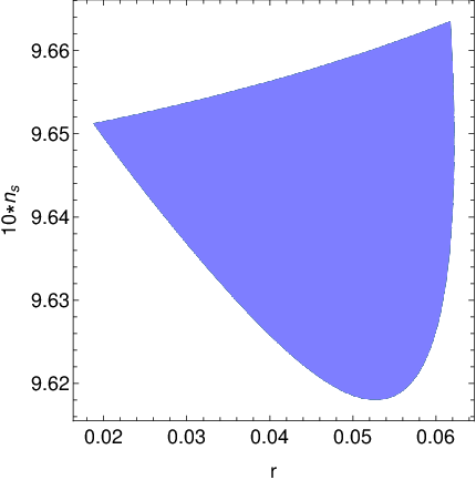
Furthermore, the running of the spectral index is defined as follows,
| (72) |
and this is constrained by Planck 2018 results as . Thus, it is also important to calculate the running of spectral index before concluding the viability of a model. By using the expression of (see Eq. (48)) and (see Eq. (45)), we get
| (73) |
To arrive to the above result, we use the horizon crossing relation of the -th mode to determine , i.e., the horizon exit time increases as the momentum of the perturbation mode decreases, as expected. Eq. (73) indicates that similarly to and , the running index () also depends on the parameters and . Taking , in Fig. 3 we give a plot of with respect to .

As it can be seen in Fig. 3, the parameter lies
within the Planck constraint for , for . For the ghost free model,
we have shown that both the pure matter bounce scenario as well as
the quasi-matter bounce scenario are consistent with the Planck
observations, what is not true in the case of scalar-tensor or
pure models. Therefore, the Lagrange multiplier ghost free
Gauss-Bonnet gravity model has a richer phenomenology as compared
to the scalar-tensor or standard gravity models, which fail
to describe in a viable way these two bounce cosmology scenarios.
Before proceeding further, it is worth mentioning that in
Cai:2016thi; Cai:2017tku, the authors explored how to build
a viable nonsingular cosmological models within the framework of
effective field theory (EFT). They showed that a healthy
nonsingular bounce model can be achieved by introducing an
effective operator of , in particular, the
effective action looks like
| (74) | |||||
where , , , and are various time dependent coefficients. Having this effective action in hand,
we like to investigate whether the model that we consider in the present paper can be embedded in or have some differences
in respect to this EFT action (). The demonstration goes as follows:
The first line in the expression (74) describes the background model and the rest is for perturbations.
Therefore the background Friedmann equations are given by,
| (75) |
Moreover the effective action (74) leads to the quadratic action for scalar and tensor perturbations as Cai:2016thi,
| (76) |
and
| (77) |
respectively, where and are scalar and tensor perturbations respectively. Moreover (s) have the following form,
| (78) |
Comparing Eqns.(11), (12) with Eqn.(75), one can argue that the background equations of our considered model can be embedded within that of the effective field theory (EFT) action (74), if the coefficients and are related with various functions of the model as,
| (79) |
and
| (80) |
respectively, recall that . Moreover comparing Eqns.(37) and (76), we may conclude that the scalar perturbation of our considered model is also consistent with that of the effective action (74), provided that the coefficients are given by,
| (81) |
where the functions are shown in Eqn.(35). However eqns.(62) and (77) clearly reveal that the tensor perturbation of the present ghost free model is not consistent with that of the effective action (74), because of the time dependence of the factor in eqn.(62), unlike in the expression of eqn.(77). At this stage it deserves mentioning that “” factor of the tensor perturbation in an effective field theory may be made time dependent if one adds the terms like or to the effective action i.e if takes the following form Cai:2016thi,
| (82) | |||||
The above effective action leads to the quadratic action of tensor perturbation as follows,
| (83) |
It is evident from eqn.(83) that due to the time dependence of , the front factor of (apart from ) becomes time dependent. Therefore the addition of the new term like in the effective action makes the “” factor of the tensor perturbation time dependent, which is consistent with our considered model. However eqn.(83) also indicates that due to the presence of the term , the gravitational wave speed in the EFT becomes different than unity, unlike to the current model where the gravitational wave speed is unity. This in turn clarifies that the present ghost free model is not consistent to the effective action (82). Thus the current Lagrange multiplier Gauss-Bonnet theory of gravity can neither be embedded within the EFT action (74) nor within the action (82). However with a non-trivial coefficient (other than unity) of Ricci scalar along with in the effective field theory action, in particular, if the EFT action has the following form Cai:2016thi,
| (84) |
then the scalar perturbed action will remain the same as in Eqn.(76), however the tensor perturbed action comes as,
| (85) |
Therefore the effective action in eqn.(84) makes the front factor of (apart from ) time dependent and also allow an unit gravitational wave speed, which are consistent to the present Lagrange multiplier Gauss-Bonnet theory of gravity. Thus the model considered in the present paper is consistent with the effective action (84) if the parameters , and satisfy the following expressions:
| (86) |
| (87) |
and
| (88) |
where is shown in Eq.(35). The first two equations (i.e Eqs.(86) and (87)) are due to matching the background equations of motion where as Eq.(88) are due to matching the tensor perturbation equation of the EFT (described by action (84)) with that of the Lagrange multiplier Gauss-Bonnet theory of gravity.
IV.3 The Energy Conditions Violation Issue for the Bounce
At this stage it deserves mentioning that apart from the computation of spacetime perturbation, the investigation of energy conditions is also important in a bouncing model from its own right as most of the bouncing models fail to rescue the null energy condition. As for example, the energy condition is violated in the bouncing scenario of Lagrange multiplier gravity model Nojiri:2019lqw, however the holonomy generalization of such F(R) model is able to rescue the null energy condition Elizalde:2019tee. Here, we want to investigate the energy conditions in the present context i.e for the bouncing scenario in the Lagrange multiplier Gauss-Bonnet theory of gravity. As we already mentioned, a crucial drawback in most of the bouncing models is the violation of the null energy condition. Here we will check the fulfillment of the energy conditions in the context of the ghost free gravity model. For this purpose, we first determine the effective energy density from Eqs. (11) and (12),
| (89) |
However, as we mentioned earlier, the energy condition has to be checked for all cosmic times, including the bouncing point which occurs at , where the low-curvature approximation no longer holds true. Thus, it will not be justified if we use the forms for the coupling function and Lagrange multiplier obtained in Eqs. (32) and (34), to check the energy condition near the bouncing point. Thereby, the best way to investigate the energy condition is to determine the forms of and for the whole range of time , and then use such forms of and in the expression of . For this purpose, we reconstruct the GB coupling function and the Lagrange multiplier term from Eqs. (19) and (17), respectively, by using the exact form of (which is valid for the entire range of the cosmic time)
| (90) |
where is an integration constant with mass dimension [+1], and we should recall that is related to by . It should be observed from the above equation that we stop at the level of the first derivative of the coupling function and we do not determine the explicit form of . However, this approximation should be sufficient, because the right hand side of Eq.(89) does not contain any term that is without a derivative of , which is also expected from the fact that the Gauss-Bonnet term without the coupling function becomes a surface integral and is eliminated from the action. Plugging back the expressions of and into Eq.(89), in Fig. 4 we give the plot of (with respect to the cosmic time), for , , (in reduced Planck units).

As can be seen in Fig. 4, becomes negative near the bouncing point. Furthermore, Eq.(89) clearly indicates that both the scalar field () and the Gauss-Bonnet term contribute to , their individual contributions being
| (91) | |||||
and
| (92) | |||||
respectively. Using these expressions we give the plot of , and (with respect to the cosmic time, for , , i.e in reduced Planck units), see Fig. [5], in order to better understand the energy flow of the universe.

Figs.[4] and [5] show that the null energy condition for the whole universe, as well as for the individual contributors, are violated, which further implies that the weak energy condition is necessarily violated. At this stage, we want to mention that the holonomy improvement is able to rescue the energy condition in the context of Lagrange multiplier F(R) gravity, as proven in Elizalde:2019tee. Hopefully, therefore, the presence of holonomy modifications even in the gravity model, or the presence of extra spatial dimensions, where is proportional to linear powers as well as quadratic powers of the energy density, may play a significant role to rescue the null energy condition for a non-singular bounce. This investigation is expected to be carried out soon in a future work.
V Conclusions
In the present paper we have considered an extended matter bounce scenario in a ghost free gravity, in particular, for the model. The idea for making the model ghost free consists in introducing a Lagrange multiplier, as discussed in Nojiri:2018ouv. In such gravity theory, we used the results of Odintsov:2019clh which indicated that the model at hand is compatible with GW170817 that this happens for a class of Gauss-Bonnet (GB) coupling functions () which satisfy the constraint equation , being the Hubble parameter. Thus, in order to make our model compatible with the event GW170817, we considered only such GB coupling functions which obey this constraint. At this stage, it is worth mentioning that this new constraint on the coupling function also fits with the equations of motion due to the presence of the scalar field potential.
In such ghost free model compatible with GW170817, we considered a non-singular bounce scenario with the scale factor being expressed as , where is a dimensionless parameter of the model and the cosmic time. For this scale factor, it was shown that, for , the spacetime perturbation modes are generated deeply in the contracting era, at large negative values of time, where the Ricci curvature is low as compared to the one in the near-bouncing era. This, in turn, makes the “low curvature limit” a viable approximation in calculating the observable quantities, which are eventually determined at the time of horizon exit. We have determined the forms of the coupling function () and Lagrange multiplier () in the low curvature regime, by using a reconstruction technique for the present model, which realizes the bouncing with the aforementioned scale factor. Such forms of and led to an explicit expression of the cosmological perturbation equation, by solving which we have determined the power spectra of the primordial perturbations and, correspondingly, have calculated the fundamental cosmological parameters, namely the spectral index of scalar perturbations, the tensor to scalar ratio, and the running spectral index, respectively.
Such observational indexes are found to depend on the dimensionless parameters of the model, as (with the Ricci curvature at the time of horizon exit) and . It turned out that the observable quantities are simultaneously compatible with the Planck 2018 constraints for the parametric range and . It should be noticed that this range of is also supported by the range , which ensures the low-curvature approximation to be a perfectly reliable one for calculating the power spectra. The expression of the spectral index we obtained clearly demonstrates that, in the absence of the GB term (the model resembling a scalar tensor one), the power spectrum becomes completely scale invariant for . This was expected, as it is well known that for a scalar tensor theory, the spectral index becomes one in a pure matter bounce scenario, which in turn makes the spectrum completely scale invariant. We recall that the pure matter bounce scenario is not consistent with observations, even in pure vacuum gravity. Here, we showed that for a ghost free model compatible with the GW170817 event, the matter as well as quasi-matter bounces may be considered as good bouncing theories, which confirms the richer bouncing phenomenology of our general model here. We further determined the effective energy density and pressure in the present context, in order to investigate the energy conditions. The energy condition has to be checked for all cosmic times, including at the bouncing point, where the low-curvature approximation no longer holds true. Thus, it will not be justified if we use the forms of coupling function and the Lagrange multiplier obtained from the low curvature approximation to check the energy condition near the bouncing point. Keeping this in mind, we have reconstructed and for the entire range of the cosmic time (by relaxing the low curvature approximation) and then used such forms of , to determine the effective energy density and pressure. As a consequence, we found that the null energy condition is violated near the bouncing point, which further implies that the weak energy condition is necessarily violated. At this stage, we want to mention that the holonomy improvement has been proven to rescue the energy conditions in the context of Lagrange multiplier gravity Elizalde:2019tee. Thus, hopefully, the presence of holonomy modifications, even in the gravity model, may similarly play a significant role to rescue the null energy conditions for a non-singular bounce. This investigation should be interesting and insightful, and we expect to carry it out in future work, soon.
Acknowledgments
EE and SDO acknowledge the support of MINECO (Spain), project FIS2016-76363-P, and AGAUR (Catalonia, Spain), project 2017 SGR 247. TP sincerely acknowledges the hospitality by ICE-CSIC/IEEC (Barcelona, Spain), where this work was done during his visit.
References
- (1) S. Nojiri, S. D. Odintsov and V. K. Oikonomou, Phys. Rev. D 99 (2019) no.4, 044050 doi:10.1103/PhysRevD.99.044050 [arXiv:1811.07790 [gr-qc]].
- (2) A.H. Guth; Phys.Rev. D23 347-356 (1981).
- (3) A. D. Linde, Contemp. Concepts Phys. 5 (1990) 1 [hep-th/0503203].
- (4) D. Langlois, hep-th/0405053.
- (5) A. Riotto, ICTP Lect. Notes Ser. 14 (2003) 317 [hep-ph/0210162].
- (6) N. Banerjee, S. Sen; Phys.Rev. D57, 4614 (1998).
- (7) J. D. Barrow and P. Saich; Class. Quantum Grav. 10, 279 (1993).
- (8) J. D. Barrow and J. P. Mimoso; Phys. Rev. D 50, 3746 (1994).
- (9) N. Banerjee and T. Paul, Eur. Phys. J. C 77 (2017) no.10, 672 doi:10.1140/epjc/s10052-017-5256-0 [arXiv:1706.05964 [hep-th]].
- (10) S. Chakraborty, T. Paul and S. SenGupta, Phys. Rev. D 98 (2018) no.8, 083539 doi:10.1103/PhysRevD.98.083539 [arXiv:1804.03004 [gr-qc]].
- (11) E. Elizalde, S. D. Odintsov, V. K. Oikonomou and T. Paul, JCAP 1902 (2019) 017 doi:10.1088/1475-7516/2019/02/017 [arXiv:1810.07711 [gr-qc]].
- (12) E. Elizalde, S. D. Odintsov, T. Paul and D. Sáez-Chillón Gómez, Phys. Rev. D 99 (2019) no.6, 063506 doi:10.1103/PhysRevD.99.063506 [arXiv:1811.02960 [gr-qc]].
- (13) S. Nojiri, S. D. Odintsov, V. K. Oikonomou, N. Chatzarakis and T. Paul, Eur. Phys. J. C 79 (2019) no.7, 565 doi:10.1140/epjc/s10052-019-7080-1 [arXiv:1907.00403 [gr-qc]].
- (14) R. H. Brandenberger, arXiv:1206.4196 [astro-ph.CO].
- (15) R. Brandenberger and P. Peter, arXiv:1603.05834 [hep-th].
- (16) D. Battefeld and P. Peter, Phys. Rept. 571 (2015) 1 doi:10.1016/j.physrep.2014.12.004 [arXiv:1406.2790 [astro-ph.CO]].
- (17) M. Novello and S. E. P. Bergliaffa, “Bouncing Cosmologies,” Phys. Rept. 463 (2008) 127 doi:10.1016/j.physrep.2008.04.006 [arXiv:0802.1634 [astro-ph]].
- (18) Y. F. Cai, Sci. China Phys. Mech. Astron. 57 (2014) 1414 doi:10.1007/s11433-014-5512-3 [arXiv:1405.1369 [hep-th]].
- (19) J. de Haro and Y. F. Cai, Gen. Rel. Grav. 47 (2015) no.8, 95 doi:10.1007/s10714-015-1936-y [arXiv:1502.03230 [gr-qc]].
- (20) S. Nojiri, S. D. Odintsov, V. K. Oikonomou and T. Paul, arXiv:1910.03546 [gr-qc].
- (21) J. L. Lehners, Class. Quant. Grav. 28 (2011) 204004 doi:10.1088/0264-9381/28/20/204004 [arXiv:1106.0172 [hep-th]].
- (22) J. L. Lehners, Phys. Rept. 465 (2008) 223 doi:10.1016/j.physrep.2008.06.001 [arXiv:0806.1245 [astro-ph]].
- (23) Y. K. E. Cheung, C. Li and J. D. Vergados, arXiv:1611.04027 [astro-ph.CO].
- (24) Y. F. Cai, A. Marciano, D. G. Wang and E. Wilson-Ewing, Universe 3 (2016) no.1, 1 doi:10.3390/Universe3010001 [arXiv:1610.00938 [astro-ph.CO]].
- (25) C. Cattoen and M. Visser, Class. Quant. Grav. 22 (2005) 4913 doi:10.1088/0264-9381/22/23/001 [gr-qc/0508045].
- (26) C. Li, R. H. Brandenberger and Y. K. E. Cheung, Phys. Rev. D 90 (2014) no.12, 123535 doi:10.1103/PhysRevD.90.123535 [arXiv:1403.5625 [gr-qc]].
- (27) D. Brizuela, G. A. D. Mena Marugan and T. Pawlowski, Class. Quant. Grav. 27 (2010) 052001 doi:10.1088/0264-9381/27/5/052001 [arXiv:0902.0697 [gr-qc]].
- (28) Y. F. Cai, E. McDonough, F. Duplessis and R. H. Brandenberger, JCAP 1310 (2013) 024 doi:10.1088/1475-7516/2013/10/024 [arXiv:1305.5259 [hep-th]].
- (29) J. Quintin, Y. F. Cai and R. H. Brandenberger, Phys. Rev. D 90 (2014) no.6, 063507 doi:10.1103/PhysRevD.90.063507 [arXiv:1406.6049 [gr-qc]].
- (30) Y. F. Cai, R. Brandenberger and P. Peter, Class. Quant. Grav. 30 (2013) 075019 doi:10.1088/0264-9381/30/7/075019 [arXiv:1301.4703 [gr-qc]].
- (31) N. J. Poplawski, Phys. Rev. D 85 (2012) 107502 doi:10.1103/PhysRevD.85.107502 [arXiv:1111.4595 [gr-qc]].
- (32) M. Koehn, J. L. Lehners and B. Ovrut, Phys. Rev. D 93 (2016) no.10, 103501 doi:10.1103/PhysRevD.93.103501 [arXiv:1512.03807 [hep-th]].
- (33) S. D. Odintsov and V. K. Oikonomou, Phys. Rev. D 92 (2015) no.2, 024016 doi:10.1103/PhysRevD.92.024016 [arXiv:1504.06866 [gr-qc]].
- (34) S. Nojiri, S. D. Odintsov and V. K. Oikonomou, Phys. Rev. D 93 (2016) no.8, 084050 doi:10.1103/PhysRevD.93.084050 [arXiv:1601.04112 [gr-qc]].
- (35) V. K. Oikonomou, Phys. Rev. D 92 (2015) no.12, 124027 doi:10.1103/PhysRevD.92.124027 [arXiv:1509.05827 [gr-qc]].
- (36) S. D. Odintsov and V. K. Oikonomou, arXiv:1512.04787 [gr-qc].
- (37) M. Koehn, J. L. Lehners and B. A. Ovrut, Phys. Rev. D 90 (2014) no.2, 025005 doi:10.1103/PhysRevD.90.025005 [arXiv:1310.7577 [hep-th]].
- (38) L. Battarra and J. L. Lehners, JCAP 1412 (2014) no.12, 023 doi:10.1088/1475-7516/2014/12/023 [arXiv:1407.4814 [hep-th]].
- (39) J. Martin, P. Peter, N. Pinto Neto and D. J. Schwarz, Phys. Rev. D 65 (2002) 123513 doi:10.1103/PhysRevD.65.123513 [hep-th/0112128].
- (40) J. Khoury, B. A. Ovrut, P. J. Steinhardt and N. Turok, Phys. Rev. D 64 (2001) 123522 doi:10.1103/PhysRevD.64.123522 [hep-th/0103239].
- (41) E. I. Buchbinder, J. Khoury and B. A. Ovrut, Phys. Rev. D 76 (2007) 123503 doi:10.1103/PhysRevD.76.123503 [hep-th/0702154].
- (42) M. G. Brown, K. Freese and W. H. Kinney, JCAP 0803 (2008) 002 doi:10.1088/1475-7516/2008/03/002 [astro-ph/0405353].
- (43) J. C. Hackworth and E. J. Weinberg, Phys. Rev. D 71 (2005) 044014 doi:10.1103/PhysRevD.71.044014 [hep-th/0410142].
- (44) S. Nojiri and S. D. Odintsov, Phys. Lett. B 637 (2006) 139 doi:10.1016/j.physletb.2006.04.026 [hep-th/0603062].
- (45) M. C. Johnson and J. L. Lehners, Phys. Rev. D 85 (2012) 103509 doi:10.1103/PhysRevD.85.103509 [arXiv:1112.3360 [hep-th]].
- (46) P. Peter and N. Pinto-Neto, Phys. Rev. D 66 (2002) 063509 doi:10.1103/PhysRevD.66.063509 [hep-th/0203013].
- (47) M. Gasperini, M. Giovannini and G. Veneziano, Phys. Lett. B 569 (2003) 113 doi:10.1016/j.physletb.2003.07.028 [hep-th/0306113].
- (48) P. Creminelli, A. Nicolis and M. Zaldarriaga, Phys. Rev. D 71 (2005) 063505 doi:10.1103/PhysRevD.71.063505 [hep-th/0411270].
- (49) J. L. Lehners and E. Wilson-Ewing, JCAP 1510 (2015) no.10, 038 doi:10.1088/1475-7516/2015/10/038 [arXiv:1507.08112 [astro-ph.CO]].
- (50) J. Mielczarek, M. Kamionka, A. Kurek and M. Szydlowski, JCAP 1007 (2010) 004 doi:10.1088/1475-7516/2010/07/004 [arXiv:1005.0814 [gr-qc]].
- (51) J. L. Lehners and P. J. Steinhardt, Phys. Rev. D 87 (2013) no.12, 123533 doi:10.1103/PhysRevD.87.123533 [arXiv:1304.3122 [astro-ph.CO]].
- (52) Y. F. Cai, J. Quintin, E. N. Saridakis and E. Wilson-Ewing, JCAP 1407 (2014) 033 doi:10.1088/1475-7516/2014/07/033 [arXiv:1404.4364 [astro-ph.CO]].
- (53) Y. F. Cai, T. Qiu, Y. S. Piao, M. Li and X. Zhang, JHEP 0710 (2007) 071 doi:10.1088/1126-6708/2007/10/071 [arXiv:0704.1090 [gr-qc]].
- (54) Y. F. Cai and E. N. Saridakis, Class. Quant. Grav. 28 (2011) 035010 doi:10.1088/0264-9381/28/3/035010 [arXiv:1007.3204 [astro-ph.CO]].
- (55) P. P. Avelino and R. Z. Ferreira, Phys. Rev. D 86 (2012) 041501 doi:10.1103/PhysRevD.86.041501 [arXiv:1205.6676 [astro-ph.CO]].
- (56) J. D. Barrow, D. Kimberly and J. Magueijo, Class. Quant. Grav. 21 (2004) 4289 doi:10.1088/0264-9381/21/18/001 [astro-ph/0406369].
- (57) J. Haro and E. Elizalde, JCAP 1510 (2015) no.10, 028 doi:10.1088/1475-7516/2015/10/028 [arXiv:1505.07948 [gr-qc]].
- (58) E. Elizalde, J. Haro and S. D. Odintsov, Phys. Rev. D 91 (2015) no.6, 063522 doi:10.1103/PhysRevD.91.063522 [arXiv:1411.3475 [gr-qc]].
- (59) A. Das, D. Maity, T. Paul and S. SenGupta, Eur. Phys. J. C 77 (2017) no.12, 813 doi:10.1140/epjc/s10052-017-5396-2 [arXiv:1706.00950 [hep-th]].
- (60) J. de Haro, JCAP 1211 (2012) 037 [arXiv:1207.3621 [gr-qc]].
- (61) E. Wilson-Ewing, JCAP 1303 (2013) 026 doi:10.1088/1475-7516/2013/03/026 [arXiv:1211.6269 [gr-qc]].
- (62) Y. F. Cai, T. t. Qiu, R. Brandenberger and X. m. Zhang, Phys. Rev. D 80 (2009) 023511 doi:10.1103/PhysRevD.80.023511 [arXiv:0810.4677 [hep-th]].
- (63) F. Finelli and R. Brandenberger, Phys. Rev. D 65 (2002) 103522 doi:10.1103/PhysRevD.65.103522 [hep-th/0112249].
- (64) Y. F. Cai, R. Brandenberger and X. Zhang, Phys. Lett. B 703 (2011) 25 doi:10.1016/j.physletb.2011.07.074 [arXiv:1105.4286 [hep-th]].
- (65) J. Haro and J. Amorós, PoS FFP 14 (2016) 163 doi:10.22323/1.224.0163 [arXiv:1501.06270 [gr-qc]].
- (66) Y. F. Cai, R. Brandenberger and X. Zhang, JCAP 1103 (2011) 003 doi:10.1088/1475-7516/2011/03/003 [arXiv:1101.0822 [hep-th]].
- (67) J. Haro and J. Amoros, JCAP 1412 (2014) no.12, 031 doi:10.1088/1475-7516/2014/12/031 [arXiv:1406.0369 [gr-qc]].
- (68) R. Brandenberger, Phys. Rev. D 80 (2009) 043516 doi:10.1103/PhysRevD.80.043516 [arXiv:0904.2835 [hep-th]].
- (69) J. de Haro and J. Amoros, JCAP 1408 (2014) 025 doi:10.1088/1475-7516/2014/08/025 [arXiv:1403.6396 [gr-qc]].
- (70) S. D. Odintsov and V. K. Oikonomou, Phys. Rev. D 90 (2014) no.12, 124083 doi:10.1103/PhysRevD.90.124083 [arXiv:1410.8183 [gr-qc]].
- (71) T. Qiu and K. C. Yang, JCAP 1011 (2010) 012 doi:10.1088/1475-7516/2010/11/012 [arXiv:1007.2571 [astro-ph.CO]].
- (72) V. K. Oikonomou, Gen. Rel. Grav. 47 (2015) no.10, 126 doi:10.1007/s10714-015-1970-9 [arXiv:1412.8195 [gr-qc]].
- (73) K. Bamba, J. de Haro and S. D. Odintsov, JCAP 1302 (2013) 008 doi:10.1088/1475-7516/2013/02/008 [arXiv:1211.2968 [gr-qc]].
- (74) A. Das, H. Mukherjee, T. Paul and S. SenGupta, Eur. Phys. J. C 78 (2018) no.2, 108 doi:10.1140/epjc/s10052-018-5603-9 [arXiv:1701.01571 [hep-th]].
- (75) S. Nojiri and S. D. Odintsov, Phys. Rept. 505 (2011) 59 doi:10.1016/j.physrep.2011.04.001 [arXiv:1011.0544 [gr-qc]].
- (76) S. Nojiri, S. D. Odintsov and V. K. Oikonomou, Phys. Rept. 692 (2017) 1 doi:10.1016/j.physrep.2017.06.001 [arXiv:1705.11098 [gr-qc]].
- (77) B. P. Abbott et al. [LIGO Scientific and Virgo and Fermi GBM and INTEGRAL and IceCube and IPN and Insight-Hxmt and ANTARES and Swift and Dark Energy Camera GW-EM and DES and DLT40 and GRAWITA and Fermi-LAT and ATCA and ASKAP and OzGrav and DWF (Deeper Wider Faster Program) and AST3 and CAASTRO and VINROUGE and MASTER and J-GEM and GROWTH and JAGWAR and CaltechNRAO and TTU-NRAO and NuSTAR and Pan-STARRS and KU and Nordic Optical Telescope and ePESSTO and GROND and Texas Tech University and TOROS and BOOTES and MWA and CALET and IKI-GW Follow-up and H.E.S.S. and LOFAR and LWA and HAWC and Pierre Auger and ALMA and Pi of Sky and DFN and ATLAS Telescopes and High Time Resolution Universe Survey and RIMAS and RATIR and SKA South Africa/MeerKAT Collaborations and AstroSat Cadmium Zinc Telluride Imager Team and AGILE Team and 1M2H Team and Las Cumbres Observatory Group and MAXI Team and TZAC Consortium and SALT Group and Euro VLBI Team and Chandra Team at McGill University], Astrophys. J. 848 (2017) no.2, L12 doi:10.3847/2041-8213/aa91c9 [arXiv:1710.05833 [astro-ph.HE]].
- (78) J. M. Ezquiaga and M. Zumalacárregui, Phys. Rev. Lett. 119 (2017) no.25, 251304 doi:10.1103/PhysRevLett.119.251304 [arXiv:1710.05901 [astro-ph.CO]].
- (79) G. Ye and Y. S. Piao, Commun. Theor. Phys. 71 (2019) no.4, 427 doi:10.1088/0253-6102/71/4/427 [arXiv:1901.02202 [gr-qc]].
- (80) J. c. Hwang and H. Noh, Phys. Rev. D 71 (2005) 063536 doi:10.1103/PhysRevD.71.063536 [gr-qc/0412126].
- (81) H. Noh and J. c. Hwang, Phys. Lett. B 515 (2001) 231 doi:10.1016/S0370-2693(01)00875-9 [astro-ph/0107069].
- (82) J. c. Hwang and H. Noh, Phys. Rev. D 66 (2002) 084009 doi:10.1103/PhysRevD.66.084009 [hep-th/0206100].
- (83) S. D. Odintsov and V. K. Oikonomou, Phys. Lett. B 797 (2019) 134874 doi:10.1016/j.physletb.2019.134874 [arXiv:1908.07555 [gr-qc]].
- (84) Y. Akrami et al. [Planck Collaboration], arXiv:1807.06211 [astro-ph.CO].
- (85) Y. Cai, Y. Wan, H. G. Li, T. Qiu and Y. S. Piao, JHEP 1701 (2017) 090 doi:10.1007/JHEP01(2017)090 [arXiv:1610.03400 [gr-qc]].
- (86) Y. Cai, H. G. Li, T. Qiu and Y. S. Piao, Eur. Phys. J. C 77 (2017) no.6, 369 doi:10.1140/epjc/s10052-017-4938-y [arXiv:1701.04330 [gr-qc]].
- (87) E. Elizalde, S. D. Odintsov and T. Paul, arXiv:1912.05138 [gr-qc].