Fixed mmWave Multi-User MIMO: Performance Analysis and Proof-of-Concept Architecture
Thanks: This research is supported by the Research Foundation Flanders (FWO), project no. S003817N (OmniDrone) and by the European Union’s Horizon 2020 under grant agreement no. 732174 (ORCA project) .

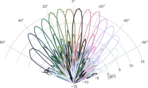
The multi-beam antenna array used in this paper is an extended prototype of the work in [6]. It features a 16x16 Butler-matrix (BM) as phase shifting network connected to a 1x16 linear antenna array. The linear antenna array is implemented on the same printed circuit board as the BM and consists of quasi-Yagi antenna elements. The operating frequency of this multi-beam array is $25$ to $30$ GHz, while the input intermediate frequency (IF) is $2.4$ GHz, up- and down-conversion is handled by the multi-beam array. This IF allows the use of cheaper off-the-shelf devices omitting expensive mmWave equipment. The BM is capable of generating spatial orthogonal beams, resulting in every beam having nulls in the directions of the main lobes of the other beams. The half power beam width of these beams is $7$ deg, the maximum beam gain is $16$ dBi and the total spatial angle range is $\pm 68$ deg. The measured antenna pattern can be seen in Fig. 1. Each of the 16 beam directions of the multi-beam array has a corresponding RF input/output port at the IF resulting in a fully connected 16x16 structure between the inputs ports and the antennas.

The KU Leuven Massive MIMO testbed, based on LTE-TDD, is used, described in detail in [7]. The testbed is configured to use $2.4$ GHz as its center frequency, which is the IF of the antenna array, and uses a $20$ MHz bandwidth. The system uses OFDM modulation with a total of 1200 subcarriers. There are two main components to this testbed, the first being the BS, which in this setup has 16 RF-chains connected to the 16 inputs of the multi-beam array. The second component are the users, in this paper we use one user and virtually add more users offline. Both components run the LabVIEW Communications MIMO Application Framework [8]. The RF chain of the user is connected to a 16-port switch [9], which can be manually controlled over a control interface by the user. Both antenna arrays are synchronised using a $11.8$ GHz clock generated by an ERASynth+ RF Signal Generator [10].

Consider a discrete memoryless channel where the received signal vector for a single user $k$ is given by

where $\mathbf{y}_{k}=[y_{1,k},\dots,y_{16,k}]$ contains the received signals at the 16 receive antennas, $p_{tx}$ is the transmit power at the BS, $\mathbf{s}$ is the transmitted signal vector as defined in (2) and $\mathbf{H}_{k}\in\mathbb{C}^{16\times 16}$ is the MIMO channel impulse response (CIR) matrix between the BS and user $k$ (see Section III-B). Readers should take note that this CIR matrix does include the multi-beam array impulse responses at both BS and UE side. $\mathbf{n}_{k}\sim\mathcal{NC}(0,\,\sigma^{2})\in\mathbb{C}^{16\times 1}$ is the normalized Gaussian noise vector at the receiver of user $k$, where $\sigma^{2}$ is the noise power. Substituting (2) in (3) gives the following received signal vector:

To receive the signal, the user selects the beam detecting the highest power using the RF switch. For user $k$, this switch is represented by the vector $\mathbf{w}^{RF}_{k}\in\mathbb{Z}_{2}^{16\times 1}$, which contains only one non-zero element dependent on the optimal beam. The received signal $y_{n,k}$ at the user $k$ after $n$-th antenna selection can then be represented as follows:

Adding the analog combining vector to the received signal vector in (4) gives us the final expression for the received signal at the user $k$:

The user and BS are in line of sight (LoS). The channel is modeled for one subcarrier resulting in a narrowband frequency flat channel. All users are located at fixed locations with a relative angle to the BS of $\theta_{bs}$. The users are rotated with an angle $\theta_{k}$ towards the BS, resulting in the following deterministic channel response for user $k$ [11]:

where $\circ$ represents the Hadamard product, $\Phi_{rx}(\theta_{k})\in\mathbb{C}^{16\times 1}$ and $\Phi_{tx}(\theta_{bs})\in\mathbb{C}^{16\times 1}$ represent the $\theta_{k}$- and $\theta_{bs}$-dependent phase shifts seen at the receiver and transmitter ULAs, respectively. These phase shifts represent both the fixed phase shifts in the BM and the angle dependent phase shifts between the antenna array elements. $\mathbf{B}(\theta_{bs},\theta_{k})\in\mathbb{C}^{16\times 16}$ represents the angle dependent channel gain matrix and can be interpreted as the macroscopic large-scale fading between all transmitting and receiving antennas. $\mathbf{B}(\theta_{bs},\theta_{k})$ also contains the antenna gains, which results in its dependency on $\theta_{bs}$ and $\theta_{k}$. Thus, $\mathbf{B}_{k}(\theta_{bs},\theta_{k})$ can be written as

where $L_{k}$ are the cable and other hardware related losses, $PL_{k}$ is the free space path loss dependent on the distance between user and BS. Where $\mathbf{g}^{tx}(\theta_{bs})=[g^{tx}_{1}(\theta_{bs}),g^{tx}_{2}(\theta_{bs}),\dots,g^{tx}_{16}(\theta_{bs})]^{T}\in\mathbb{C}^{16\times 1}$ is the transmitter antenna gain vector towards user $k$. Each element $g^{tx}_{m}(\theta_{bs})$ represents the gain of antenna $m$ towards user $k$ dependent on the azimuth angle $\theta_{bs}$ of the user to the BS. Similarly, $\mathbf{g}^{rx}(\theta_{k})\in\mathbb{C}^{16\times 1}$ consists of the $\theta_{k}$-dependent antenna gains of the receiver multi-beam array.

To increase further readability, we omit the $\theta_{bs}$ and $\theta_{k}$ dependency in the notation of the channel impulse response matrix and shorten it to $\mathbf{H}_{k}$. As the user $k$ uses only one of its receiving antennas, we can simplify the channel matrix $\mathbf{H}_{k}$ to a channel vector $\mathbf{h}_{k}$ by applying the user’s combining vector $\mathbf{w}^{RF}_{k}$. This vector $\mathbf{h}_{k}$ contains only one antenna beam of the user side multi-beam antenna array. The simplified channel vector $\mathbf{h}_{k}\in\mathbb{C}^{16\times 1}$ is then defined as follows

Take note that this is the format of the channel that the BS will retrieve from its channel estimation.

For the calculation of the digital precoder at the BS, the CIR is necessary. The CIR can be gathered at the BS side by several different channel estimation techniques, for example using minimum mean squared error channel estimation defined in Theorem 3.1 in [11]. However, these estimated channels do contain estimation errors and are thus indicated by $\mathbf{\hat{h}}_{k}$ to differentiate them from the real channel $\mathbf{h}_{k}$.

In this paper, we consider three digital precoding techniques, namely Maximum Ratio (MR) precoding, Zero Forcing (ZF) and Regularized Zero Forcing (RZF). These techniques are based on their corresponding combining matrices as defined in [11]. The precoding vector for the $k$-th user can be calculated as follows:

where $\mathbf{w}^{BB}_{k}$ is one vector of the digital combining matrix at the BS: $\mathbf{W}^{BB}=[\mathbf{w}^{BB}_{1},\dots,\mathbf{w}^{BB}_{k}]$. This combining matrix is calculated using the CIR of all users: $\mathbf{\hat{H}}=[\mathbf{\hat{h}}_{1},\dots,\mathbf{\hat{h}}_{k}]\in\mathbb{C}^{16\times K}$. A short overview of these three techniques is given, for a more detailed description we refer to [11]:

• •

  MR maximizes the received signal to all users, $\mathbf{W}^{BB}\in\mathbb{C}^{16\times K}$ is defined as follows

  $$\mathbf{W}^{BB,MR}=\mathbf{\hat{H}}.$$

  (11)

  This precoding technique is often used due to its low complexity.

• •

  ZF attempts to cancel all intra-cell interference. The combining matrix is defined as

  $$\mathbf{W}^{BB,ZF}=\mathbf{\hat{H}}((\mathbf{\hat{H}})^{H}\mathbf{\hat{H}})^{-1}.$$

  (12)

• •

  RZF makes a trade-off between noise and intra-cell interference. The combining matrix is defined as follows

  $$\mathbf{W}^{BB,RZF}=\mathbf{\hat{H}}((\mathbf{\hat{H}})^{H}\mathbf{\hat{H}}+\sigma^{2}\mathbf{P}_{tx}^{-1})^{-1},$$

  (13)

  where $\mathbf{P}_{tx}=diag(p_{tx},\dots,p_{tx})\in\mathbb{C}^{16\times 16}$ is a diagonal matrix containing the transmit power to each user and $\sigma^{2}$ is the noise power.

To verify the performance of the proposed system, we evaluate the downlink spectral efficiency (SE) expressed in bps/Hz. A single cell system is considered and the individual downlink SE for user $k$ is as follows

where $SINR^{DL}_{k}$ is the downlink Signal-to-Interference-and-Noise-Ratio (SINR) for the user $k$ and $\frac{\tau_{d}}{\tau_{c}}$ is the fraction of samples per coherence block that is used for downlink data. The $SINR^{DL}_{k}$ is defined as follows:

where $\mathbf{H}_{k}$ is the real channel matrix for user $k$ as defined in (7), $\mathbf{f}^{BB}_{k}$ the digital baseband precoding vector for user $k$ as defined in (1) and $\sigma_{DL}^{2}$ being the average noise power.

We can also evaluate the summed SE per cell, expressed in bps/Hz/cell. Which is calculated by summing the individual SE of all users within one cell:

The individual spectral efficiency can be seen in Fig. 3. The median value gives an indication of the average performance of the system while the distance between the lower and the upper quartile gives an indication of the fairness of the system. A fair system has a small spread of its individual SE.

When using MR precoding, the patch antenna array always performs better in terms of individual SE, thus we can conclude that a classic array of patch antennas is the most efficient option when MR precoding is considered. However, both ZF and RZF generally outperform the Analog and MR precoders and they have similar performance for a low amount of users for both arrays. However, for a number of users equal to the number of antennas, ZF’s performance starts to degrade, especially if we consider fairness. The measured system is almost always fairer than the simulated system, except for analog beamforming. ZF and RZF perform similar for the beamforming array, this could be due to the limited noise power. If a larger bandwidth is considered, then RZF should outperform ZF due to its noise compensation. We can conclude that the patch and beamforming antenna arrays are both efficient for low number of users. However, if we want to serve a high number of users similar to the number of antennas, then a directive antenna array proves more efficient and fair, ideally using RZF precoding.

When the summed SE is considered for analog and MR precoding, we can draw similar conclusions as when individual SE is analyzed. The only difference is that the system performance is independent of the number of users. Fig. 4 shows the mean summed SE per cell for different numbers of users using ZF and RZF. The patch and beamforming antenna arrays show a similar performance for up to eight users. For a larger number of users, the patch array’s performance degrades faster than the beamforming antenna array’s for both ZF and RZF. This confirms the conclusion that for a number of users similar to the number of antennas, the beamforming antenna array outperforms the patch antenna array. The performance of the simulated antenna array approximates on average the measured results. This verifies that the proposed model accurately reproduces the behavior of the real system.

References

- [1] WWRF, “Wireless to the X: Extend 5G to Wireless Broadband Access,” White Paper, Nov 2017.
- [2] Y. Niu, Y. Li, D. Jin, L. Su, and A. V. Vasilakos, “A survey of millimeter wave communications (mmWave) for 5G: opportunities and challenges,” Wireless Networks, vol. 21, no. 8, pp. 2657–2676, Nov 2015.
- [3] A. Colpaert, E. Vinogradov, and S. Pollin, “Aerial Coverage Analysis of Cellular Systems at LTE and mmWave Frequencies Using 3D City Models,” Sensors, vol. 18, no. 12, 2018.
- [4] I. Ahmed, H. Khammari, A. Shahid, A. Musa, K. S. Kim, E. De Poorter, and I. Moerman, “A Survey on Hybrid Beamforming Techniques in 5G: Architecture and System Model Perspectives,” IEEE Communications Surveys Tutorials, vol. 20, no. 4, pp. 3060–3097, Fourthquarter 2018.
- [5] J. Jang, M. Chung, S. C. Hwang, Y. Lim, H. Yoon, T. Oh, B. Min, Y. Lee, K. S. Kim, C. Chae, and D. K. Kim, “Smart Small Cell with Hybrid Beamforming for 5G: Theoretical Feasibility and Prototype Results,” IEEE Wireless Communications, vol. 23, no. 6, pp. 124–131, Dec 2016.
- [6] X. Wang, M. Laabs, D. Plettemeier, K. Kosaka, and Y. Matsunaga, “28 GHz Multi-Beam Antenna Array based on Wideband High-dimension 16x16 Butler Matrix,” in 2019 13th European Conference on Antennas and Propagation (EuCAP), Mar 2019, pp. 1–4.
- [7] C. Chen, V. Volski, L. Van der Perre, G. A. E. Vandenbosch, and S. Pollin, “Finite Large Antenna Arrays for Massive MIMO: Characterization and System Impact,” IEEE Transactions on Antennas and Propagation, vol. 65, no. 12, pp. 6712–6720, Dec 2017.
- [8] National-Instruments, “5G Massive MIMO Testbed: From Theory to Reality,” White Paper, 2017.
- [9] Mini-Circuits, “USB-1SP16T-83H usb / ttl rf sp16t switch,” Datasheet, New York, USA, Dec 2017.
- [10] Era-Instruments, “ERASynth: An Open Source, Arduino-Compatible RF Signal Generator with Wi-Fi Connectivity,” Datasheet, Istanbul, Turkey, Apr 2019.
- [11] E. Björnson, J. Hoydis, and L. Sanguinetti, “Massive MIMO networks: Spectral, energy, and hardware efficiency,” Foundations and Trends® in Signal Processing, vol. 11, no. 3-4, pp. 154–655, 2017.