Searching Central Difference Convolutional Networks for Face Anti-Spoofing
Abstract
Face anti-spoofing (FAS) plays a vital role in face recognition systems. Most state-of-the-art FAS methods 1) rely on stacked convolutions and expert-designed network, which is weak in describing detailed fine-grained information and easily being ineffective when the environment varies (e.g., different illumination), and 2) prefer to use long sequence as input to extract dynamic features, making them difficult to deploy into scenarios which need quick response. Here we propose a novel frame level FAS method based on Central Difference Convolution (CDC), which is able to capture intrinsic detailed patterns via aggregating both intensity and gradient information. A network built with CDC, called the Central Difference Convolutional Network (CDCN), is able to provide more robust modeling capacity than its counterpart built with vanilla convolution. Furthermore, over a specifically designed CDC search space, Neural Architecture Search (NAS) is utilized to discover a more powerful network structure (CDCN++), which can be assembled with Multiscale Attention Fusion Module (MAFM) for further boosting performance. Comprehensive experiments are performed on six benchmark datasets to show that 1) the proposed method not only achieves superior performance on intra-dataset testing (especially 0.2% ACER in Protocol-1 of OULU-NPU dataset), 2) it also generalizes well on cross-dataset testing (particularly 6.5% HTER from CASIA-MFSD to Replay-Attack datasets). The codes are available at https://github.com/ZitongYu/CDCN.
1 Introduction

Face recognition has been widely used in many interactive artificial intelligence systems for its convenience. However, vulnerability to presentation attacks (PA) curtail its reliable deployment. Merely presenting printed images or videos to the biometric sensor could fool face recognition systems. Typical examples of presentation attacks are print, video replay, and 3D masks. For the reliable use of face recognition systems, face anti-spoofing (FAS) methods are important to detect such presentation attacks.
In recent years, several hand-crafted features based boulkenafet2015face; Boulkenafet2017Face; Pereira2012LBP; Komulainen2014Context; Peixoto2011Face; Patel2016Secure and deep learning based qin2019learning; yu2020auto; Liu2018Learning; jourabloo2018face; yang2019face; Atoum2018Face; Gan20173D; george2019deep methods have been proposed for presentation attack detection (PAD). On one hand, the classical hand-crafted descriptors (e.g., local binary pattern (LBP) boulkenafet2015face) leverage local relationship among the neighbours as the discriminative features, which is robust for describing the detailed invariant information (e.g., color texture, moir pattern and noise artifacts) between the living and spoofing faces. On the other hand, due to the stacked convolution operations with nonlinear activation, the convolutional neural networks (CNN) hold strong representation abilities to distinguish the bona fide and PA. However, CNN based methods focus on the deeper semantic features, which are weak in describing detailed fine-grained information between living and spoofing faces and easily being ineffective when the environment varies (e.g., different light illumination). How to integrate local descriptors with convolution operation for robust feature representation is worth exploring.
Most recent deep learning based FAS methods are usually built upon image classification task based backbones yang2014learn; yang2019face; george2019deep, such as VGG simonyan2014very, ResNet he2016deep and DenseNet huang2017densely. The networks are usually supervised by binary cross-entropy loss, which easily learns the arbitrary patterns such as screen bezel instead of the nature of spoofing patterns. In order to solve this issue, several depth supervised FAS methods Atoum2018Face; Liu2018Learning, which utilize pseudo depth map label as auxiliary supervised signal, have been developed. However, all these network architectures are carefully designed by human experts, which might not be optimal for FAS task. Hence, to automatically discover best-suited networks for FAS task with auxiliary depth supervision should be considered.
Most existing state-of-the-art FAS methods Liu2018Learning; wang2018exploiting; yang2019face; lin2019face need multiple frames as input to extract dynamic spatio-temporal features (e.g., motion Liu2018Learning; wang2018exploiting and rPPG yang2019face; lin2019face) for PAD. However, long video sequence may not be suitable for specific deployment conditions where the decision needs to be made quickly. Hence, frame level PAD approaches are advantageous from the usability point of view despite inferior performance compared with video level methods. To design high-performing frame level methods is crucial for real-world FAS applications.
Motivated by the discussions above, we propose a novel convolution operator called Central Difference Convolution (CDC), which is good at describing fine-grained invariant information. As shown in Fig. 1, CDC is more likely to extract intrinsic spoofing patterns (e.g., lattice artifacts) than vanilla convolution in diverse environments. Furthermore, over a specifically designed CDC search space, Neural Architecture Search (NAS) is utilized to discover the excellent frame level networks for depth supervised face anti-spoofing task. Our contributions include:
- •
We design a novel convolution operator called Central Difference Convolution (CDC), which is suitable for FAS task due to its remarkable representation ability for invariant fine-grained features in diverse environments. Without introducing any extra parameters, CDC can replace the vanilla convolution and plug and play in existing neural networks to form Central Difference Convolutional Networks (CDCN) with more robust modeling capacity.
- •
We propose CDCN++, an extended version of CDCN, consisting of the searched backbone network and Multiscale Attention Fusion Module (MAFM) for aggregating the multi-level CDC features effectively.
- •
To our best knowledge, this is the first approach that searches neural architectures for FAS task. Different from the previous classification task based NAS supervised by softmax loss, we search the well-suited frame level networks for depth supervised FAS task over a specifically designed CDC search space.
- •
Our proposed method achieves state-of-the-art performance on all six benchmark datasets with both intra- as well as cross-dataset testing.
2 Related Work
Face Anti-Spoofing. Traditional face anti-spoofing methods usually extract hand-crafted features from the facial images to capture the spoofing patterns. Several classical local descriptors such as LBP boulkenafet2015face; Pereira2012LBP, SIFT Patel2016Secure, SURF Boulkenafet2017Face_SURF, HOG Komulainen2014Context and DoG Peixoto2011Face are utilized to extract frame level features while video level methods usually capture dynamic clues like dynamic texture komulainen2012face, micro-motion siddiqui2016face and eye blinking Pan2007Eyeblink. More recently, a few deep learning based methods are proposed for both frame level and video level face anti-spoofing. For frame level methods Li2017An; Patel2016Cross; george2019deep; jourabloo2018face, pre-trained deep CNN models are fine-tuned to extract features in a binary-classification setting. In contrast, auxiliary depth supervised FAS methods Atoum2018Face; Liu2018Learning are introduced to learn more detailed information effectively. On the other hand, several video level CNN methods are presented to exploit the dynamic spatio-temporal wang2018exploiting; yang2019face; lin2018live or rPPG li2016generalized; Liu2018Learning; lin2019face features for PAD. Despite achieving state-of-the-art performance, video level deep learning based methods need long sequence as input. In addition, compared with traditional descriptors, CNN overfits easily and is hard to generalize well on unseen scenes.
Convolution Operators. The convolution operator is commonly used in extracting basic visual features in deep learning framework. Recently extensions to the vanilla convolution operator have been proposed. In one direction, classical local descriptors (e.g., LBP ahonen2006face and Gabor filters jain1991unsupervised) are considered into convolution design. Representative works include Local Binary Convolution juefei2017local and Gabor Convolution luan2018gabor, which is proposed for saving computational cost and enhancing the resistance to the spatial changes, respectively. Another direction is to modify the spatial scope for aggregation. Two related works are dialated convolution yu2015multi and deformable convolution dai2017deformable. However, these convolution operators may not be suitable for FAS task because of the limited representation capacity for invariant fine-grained features.
Neural Architecture Search. Our work is motivated by recent researches on NAS brock2017smash; dong2019searching; liu2018darts; pham2018efficient; zoph2016neural; zoph2018learning; xu2019pc, while we focus on searching for a depth supervised model with high performance instead of a binary classification model for face anti-spoofing task. There are three main categories of existing NAS methods: 1) Reinforcement learning based zoph2016neural; zoph2018learning, 2) Evolution algorithm based real2019regularized; real2017large, and 3) Gradient based liu2018darts; xu2019pc; cai2019proxylessnas. Most of NAS approaches search networks on a small proxy task and transfer the found architecture to another large target task. For the perspective of computer vision applications, NAS has been developed for face recognition zhu2019neural, action recognition peng2019video, person ReID quan2019auto, object detection ghiasi2019fpn and segmentation zhang2019customizable tasks. To the best of our knowledge, no NAS based method has ever been proposed for face anti-spoofing task.
In order to overcome the above-mentioned drawbacks and fill in the blank, we search the frame level CNN over a specially designed search space with the new proposed convolution operator for depth-supervised FAS task.
3 Methodology
In this section, we will first introduce our Central Difference Convolution in Section 3.1, then introduce the Central Difference Convolutional Networks (CDCN) for face anti-spoofing in Section 3.2, and at last present the searched networks with attention mechanism (CDCN++) in Section 3.3.
3.1 Central Difference Convolution
In modern deep learning frameworks, the feature maps and convolution are represented in 3D shape (2D spatial domain and extra channel dimension). As the convolution operation remains the same across the channel dimension, for simplicity, in this subsection the convolutions are described in 2D while extension to 3D is straightforward.
Vanilla Convolution. As 2D spatial convolution is the basic operation in CNN for vision tasks, here we denote it as vanilla convolution and review it shortly first. There are two main steps in the 2D convolution: 1) sampling local receptive field region over the input feature map ; 2) aggregation of sampled values via weighted summation. Hence, the output feature map can be formulated as
| (1) |
where denotes current location on both input and output feature maps while enumerates the locations in . For instance, local receptive field region for convolution operation with 33 kernel and dilation 1 is .
Vanilla Convolution Meets Central Difference. Inspired by the famous local binary pattern (LBP) boulkenafet2015face which describes local relations in a binary central difference way, we also introduce central difference into vanilla convolution to enhance its representation and generalization capacity. Similarly, central difference convolution also consists of two steps, i.e., sampling and aggregation. The sampling step is similar to that in vanilla convolution while the aggregation step is different: as illustrated in Fig. 2, central difference convolution prefers to aggregate the center-oriented gradient of sampled values. Eq. (1) becomes
| (2) |
When , the gradient value always equals to zero with respect to the central location itself.
For face anti-spoofing task, both the intensity-level semantic information and gradient-level detailed message are crucial for distinguishing the living and spoofing faces, which indicates that combining vanilla convolution with central difference convolution might be a feasible manner to provide more robust modeling capacity. Therefore we generalize central difference convolution as
| (3) |
where hyperparameter tradeoffs the contribution between intensity-level and gradient-level information. The higher value of means the more importance of central difference gradient information. We will henceforth refer to this generalized Central Difference Convolution as CDC, which should be easy to identify according to its context.
Implementation for CDC. In order to efficiently implement CDC in modern deep learning framework, we decompose and merge Eq. (3) into the vanilla convolution with additional central difference term
| (4) |
According to the Eq. (4), CDC can be easily implemented by a few lines of code in PyTorchpaszke2017automatic and TensorFlowabadi2016tensorflow. The derivation of Eq. (4) and codes based on Pytorch are shown in Appendix A.
Relation to Prior Work. Here we discuss the relations between CDC and vanilla convolution, local binary convolutionjuefei2017local and gabor convolutionluan2018gabor, which share similar design philosophy but with different focuses. The ablation study is in Section 4.3 to show superior performance of CDC for face anti-spoofing task.
Relation to Vanilla Convolution. CDC is more generalized. It can be seen from Eq. (3) that vanilla convolution is a special case of CDC when , i.e., aggregating local intensity information without gradient message.
Relation to Local Binary Convolutionjuefei2017local. Local binary convolution (LBConv) focuses on computational reduction so its modeling capacity is limited. CDC focuses on enhancing rich detailed feature representation capacity without any additional parameters. On the other side, LBConv uses pre-defined filters to describe the local feature relation while CDC can learn these filters automatically.
Relation to Gabor Convolutionluan2018gabor. Gabor convolution (GaborConv) devotes to enhancing the representation capacity of spatial transformations (i.e., orientation and scale changes) while CDC focuses more on representing fine-grained robust features in diverse environments.
3.2 CDCN
Depth-supervised face anti-spoofing methods Liu2018Learning; Atoum2018Face take advantage of the discrimination between spoofing and living faces based on 3D shape, and provide pixel-wise detailed information for the FAS model to capture spoofing cues. Motivated by this, a similar depth-supervised network Liu2018Learning called “DepthNet” is built up as baseline in this paper. In order to extract more fine-grained and robust features for estimating the facial depth map, CDC is introduced to form Central Difference Convolutional Networks (CDCN). Note that DepthNet is the special case of the proposed CDCN when for all CDC operators.
The details of CDCN are shown in Table 1. Given a single RGB facial image with size , multi-level (low-level, mid-level and high-level) fused features are extracted for predicting the grayscale facial depth with size . We use as the default setting and ablation study about will be shown in Section 4.3.
For the loss function, mean square error loss is utilized for pixel-wise supervision. Moreover, for the sake of fine-grained supervision needs in FAS task, contrastive depth loss wang2018exploiting is considered to help the networks learn more detailed features. So the overall loss can be formulated as .
| Level | Output | DepthNet Liu2018Learning | CDCN () |
|---|---|---|---|
| Low | |||
| Mid | |||
| High | |||
| [concat (Low, Mid, High), ] | |||
| # params | |||
3.3 CDCN++
It can be seen from Table 1 that the architecture of CDCN is designed coarsely (e.g., simply repeating the same block structure for different levels), which might be sub-optimized for face anti-spoofing task. Inspired by the classical visual object understanding models palmeri2004visual, we propose an extended version CDCN++ (see Fig. 5), which consists of a NAS based backbone and Multiscale Attention Fusion Module (MAFM) with selective attention capacity.
Search Backbone for FAS task. Our searching algorithm is based on two gradient-based NAS methods liu2018darts; xu2019pc, and more technical details can be referred to the original papers. Here we mainly state the new contributions about searching backbone for FAS task.
As illustrated in Fig. 3(a), the goal is to search for cells in three levels (low-level, mid-level and high-level) to form a network backbone for FAS task. Inspired by the dedicated neurons for hierarchical organization in human visual system palmeri2004visual, we prefer to search these multi-level cells freely (i.e., cells with varied structures), which is more flexible and generalized. We name this configuration as “Varied Cells” and will study its impacts in Sec. 4.3 (see Tab. 2). Different from previous works liu2018darts; xu2019pc, we adopt only one output of the latest incoming cell as the input of the current cell.
As for the cell-level structure, Fig. 3(b) shows that each cell is represented as a directed acyclic graph (DAG) of nodes , where each node represents a network layer. We denote the operation space as , and Fig. 3(c) shows eight designed candidate operations (none, skip-connect and CDCs). Each edge of DAG represents the information flow from node to node , which consists of the candidate operations weighted by the architecture parameter . Specially, each edge can be formulated by a function where . Softmax function is utilized to relax architecture parameter into operation weight , that is . The intermediate node can be denoted as and the output node is represented by weighted summation of all intermediate nodes . Here we propose a node attention strategy to learn the importance weights among intermediate nodes, that is , where is the softmax of the original learnable weight for intermediate node .

In the searching stage, and are denoted as the training and validation loss respectively, which are all based on the depth-supervised loss described in Sec. 3.2. Network parameters and architecture parameters are learned with the following bi-level optimization problem:
| (5) |
After convergence, the final discrete architecture is derived by: 1) setting ; 2) for each intermediate node, choosing one incoming edge with the largest value of , and 3) for each output node, choosing the one incoming intermediate node with largest value of (denoted as “Node Attention”) as input. In contrast, choosing last intermediate node as output node is more straightforward. We will compare these two settings in Sec. 4.3 (see Tab. 2).
MAFM. Although simply fusing low-mid-high levels features can boost performance for the searched CDC architecture, it is still hard to find the important regions to focus, which goes against learning more discriminative features. Inspired by the selective attention in human visual system palmeri2004visual; ungerleider2000mechanisms, neurons at different levels are likely to have stimuli in their receptive fields with various attention. Here we propose a Multiscale Attention Fusion Module (MAFM), which is able to refine and fuse low-mid-high levels CDC features via spatial attention.
As illustrated in Fig. 4, features from different levels are refined via spatial attention woo2018cbam with receptive fields related kernel size (i.e., the high/semantic level should be with small attention kernel size while low level with large attention kernel size in our case) and then concatenate together. The refined features can be formulated as
| (6) |
where represents Hadamard product. and denotes avg and max pool layer respectively. means the sigmoid function while is the convolution layer. Vanilla convolutions with 77, 55 and 33 kernels are utilized for , and , respectively. CDC is not chosen here because of its limited capacity of global semantic cognition, which is vital in spatial attention. The corresponding ablation study is conducted in Sec. 4.3.

4 Experiments
In this section, extensive experiments are performed to demonstrate the effectiveness of our method. In the following, we sequentially describe the employed datasets & metrics (Sec. 4.1), implementation details (Sec. 4.2), results (Sec. 4.3 - 4.5) and analysis (Sec. 4.6).
4.1 Datasets and Metrics
Databases. Six databases OULU-NPU Boulkenafet2017OULU, SiW Liu2018Learning, CASIA-MFSD Zhang2012A, Replay-Attack ReplayAttack, MSU-MFSD wen2015face and SiW-M liu2019deep are used in our experiments. OULU-NPU and SiW are high-resolution databases, containing four and three protocols to validate the generalization (e.g., unseen illumination and attack medium) of models respectively, which are utilized for intra testing. CASIA-MFSD, Replay-Attack and MSU-MFSD are databases which contain low-resolution videos, which are used for cross testing. SiW-M is designed for cross-type testing for unseen attacks as there are rich (13) attacks types inside.
Performance Metrics. In OULU-NPU and SiW dataset, we follow the original protocols and metrics, i.e., Attack Presentation Classification Error Rate (APCER), Bona Fide Presentation Classification Error Rate (BPCER), and ACER ACER for a fair comparison. Half Total Error Rate (HTER) is adopted in the cross testing between CASIA-MFSD and Replay-Attack. Area Under Curve (AUC) is utilized for intra-database cross-type test on CASIA-MFSD, Replay-Attack and MSU-MFSD. For the cross-type test on SiW-M, APCER, BPCER, ACER and Equal Error Rate (EER) are employed.
4.2 Implementation Details
Depth Generation. Dense face alignment PRNet Feng2018Joint is adopted to estimate the 3D shape of the living face and generate the facial depth map with size . More details and samples can be found in wang2018exploiting. To distinguish living faces from spoofing faces, at the training stage, we normalize living depth map in a range of , while setting spoofing depth map to 0, which is similar to Liu2018Learning.
Training and Testing Setting. Our proposed method is implemented with Pytorch. In the training stage, models are trained with Adam optimizer and the initial learning rate (lr) and weight decay (wd) are 1e-4 and 5e-5, respectively. We train models with maximum 1300 epochs while lr halves every 500 epochs. The batch size is 56 on eight 1080Ti GPUs. In the testing stage, we calculate the mean value of the predicted depth map as the final score.
Searching Setting. Similar to xu2019pc, partial channel connection and edge normalization are adopted. The initial number of channel is sequentially in the network (see Fig. 3(a)), which doubles after searching. Adam optimizer with lr=1e-4 and wd=5e-5 is utilized when training the model weights. The architecture parameters are trained with Adam optimizer with lr=6e-4 and wd=1e-3. We search 60 epochs on Protocol-1 of OULU-NPU with batchsize 12 while architecture parameters are not updated in the first 10 epochs. The whole process costs one day on three 1080Ti.
4.3 Ablation Study
In this subsection, all ablation studies are conducted on Protocol-1 (different illumination condition and location between train and test sets) of OULU-NPU Boulkenafet2017OULU to explore the details of our proposed CDC, CDCN and CDCN++.

Impact of in CDCN. According to Eq. (3), controls the contribution of the gradient-based details, i.e., the higher , the more local detailed information included. As illustrated in Fig. 6(a), when , CDC always achieves better performance than vanilla convolution (, ACER=3.8%), indicating the central difference based fine-grained information is helpful for FAS task. As the best performance (ACER=1.0%) is obtained when , we use this setting for the following experiments. Besides keeping the constant for all layers, we also explore an adaptive CDC method to learn for every layer, which is shown in Appendix B.
CDC vs. Other Convolutions. As discussed in Sec. 3.1 about the relation between CDC and prior convolutions, we argue that the proposed CDC is more suitable for FAS task as the detailed spoofing artifacts in diverse environments should be represented by the gradient-based invariant features. Fig. 6(b) shows that CDC outperforms other convolutions by a large margin (more than 2% ACER). It is interesting to find that LBConv performs better than vanilla convolution, indicating that the local gradient information is important for FAS task. GaborConv performs the worst because it is designed for capturing spatial invariant features, which is not helpful in face anti-spoofing task.
| Model | Varied cells | Node attention | ACER(%) |
|---|---|---|---|
| NAS_Model 1 | 1.7 | ||
| NAS_Model 2 | 1.5 | ||
| NAS_Model 3 | 1.4 | ||
| NAS_Model 4 | 1.3 |
Impact of NAS Configuration. Table 2 shows the ablation study about the two NAS configurations described in Sec. 3.3, i.e., varied cells and node attention. Compared to the baseline setting with the shared cells and last intermediate node as output node, both these two configurations can boost the searching performance. The reason behind is twofold: 1) with more flexible searching constraints, NAS is able to find dedicated cells for different levels, which is more similar to human visual system palmeri2004visual, and 2) taking the last intermediate node as output might not be optimal while choosing the most important one is more reasonable.
| Backbone | Multi-level Fusion | ACER(%) |
|---|---|---|
| w/o NAS | w/ multi-level concat | 1.0 |
| w/ NAS | w/ multi-level concat | 0.7 |
| w/ NAS | w/ MAFM (3x3,3x3,3x3 CDC) | 1.2 |
| w/ NAS | w/ MAFM (3x3,3x3,3x3 VanillaConv) | 0.6 |
| w/ NAS | w/ MAFM (5x5,5x5,5x5 VanillaConv) | 1.1 |
| w/ NAS | w/ MAFM (7x7,5x5,3x3 VanillaConv) | 0.2 |
| Prot. | Method | APCER(%) | BPCER(%) | ACER(%) |
|---|---|---|---|---|
| 1 | GRADIANT boulkenafet2017competition | 1.3 | 12.5 | 6.9 |
| STASN yang2019face | 1.2 | 2.5 | 1.9 | |
| Auxiliary Liu2018Learning | 1.6 | 1.6 | 1.6 | |
| FaceDs jourabloo2018face | 1.2 | 1.7 | 1.5 | |
| FAS-TD wang2018exploiting | 2.5 | 0.0 | 1.3 | |
| DeepPixBiS george2019deep | 0.8 | 0.0 | 0.4 | |
| CDCN (Ours) | 0.4 | 1.7 | 1.0 | |
| CDCN++ (Ours) | 0.4 | 0.0 | 0.2 | |
| 2 | DeepPixBiS george2019deep | 11.4 | 0.6 | 6.0 |
| FaceDs jourabloo2018face | 4.2 | 4.4 | 4.3 | |
| Auxiliary Liu2018Learning | 2.7 | 2.7 | 2.7 | |
| GRADIANT boulkenafet2017competition | 3.1 | 1.9 | 2.5 | |
| STASN yang2019face | 4.2 | 0.3 | 2.2 | |
| FAS-TD wang2018exploiting | 1.7 | 2.0 | 1.9 | |
| CDCN (Ours) | 1.5 | 1.4 | 1.5 | |
| CDCN++ (Ours) | 1.8 | 0.8 | 1.3 | |
| 3 | DeepPixBiS george2019deep | 11.719.6 | 10.614.1 | 11.19.4 |
| FAS-TD wang2018exploiting | 5.91.9 | 5.93.0 | 5.91.0 | |
| GRADIANT boulkenafet2017competition | 2.63.9 | 5.05.3 | 3.82.4 | |
| FaceDs jourabloo2018face | 4.01.8 | 3.81.2 | 3.61.6 | |
| Auxiliary Liu2018Learning | 2.71.3 | 3.11.7 | 2.91.5 | |
| STASN yang2019face | 4.73.9 | 0.91.2 | 2.81.6 | |
| CDCN (Ours) | 2.41.3 | 2.22.0 | 2.31.4 | |
| CDCN++ (Ours) | 1.71.5 | 2.01.2 | 1.80.7 | |
| 4 | DeepPixBiS george2019deep | 36.729.7 | 13.314.1 | 25.012.7 |
| GRADIANT boulkenafet2017competition | 5.04.5 | 15.07.1 | 10.05.0 | |
| Auxiliary Liu2018Learning | 9.35.6 | 10.46.0 | 9.56.0 | |
| FAS-TD wang2018exploiting | 14.28.7 | 4.23.8 | 9.23.4 | |
| STASN yang2019face | 6.710.6 | 8.38.4 | 7.54.7 | |
| FaceDs jourabloo2018face | 1.26.3 | 6.15.1 | 5.65.7 | |
| CDCN (Ours) | 4.64.6 | 9.28.0 | 6.92.9 | |
| CDCN++ (Ours) | 4.23.4 | 5.84.9 | 5.02.9 |
Effectiveness of NAS Based Backbone and MAFM. The proposed CDCN++, consisting of NAS based backbone and MAFM, is shown in Fig. 5. It is obvious that cells from multiple levels are quite different and the mid-level cell has deeper (four CDC) layers. Table 3 shows the ablation studies about NAS based backbone and MAFM. It can be seen from the first two rows that NAS based backbone with direct multi-level fusion outperforms (0.3% ACER) the backbone without NAS, indicating the effectiveness of our searched architecture. Meanwhile, backbone with MAFM achieves 0.5% ACER lower than that with direct multi-level fusion, which shows the effectiveness of MAFM. We also analyse the convolution type and kernel size in MAFM and find that vanilla convolution is more suitable for capturing the semantic spatial attention. Besides, the attention kernel size should be large (7x7) and small (3x3) enough for low-level and high-level features, respectively.
| Prot. | Method | APCER(%) | BPCER(%) | ACER(%) |
|---|---|---|---|---|
| 1 | Auxiliary Liu2018Learning | 3.58 | 3.58 | 3.58 |
| STASN yang2019face | – | – | 1.00 | |
| FAS-TD wang2018exploiting | 0.96 | 0.50 | 0.73 | |
| CDCN (Ours) | 0.07 | 0.17 | 0.12 | |
| CDCN++ (Ours) | 0.07 | 0.17 | 0.12 | |
| 2 | Auxiliary Liu2018Learning | 0.570.69 | 0.570.69 | 0.570.69 |
| STASN yang2019face | – | – | 0.280.05 | |
| FAS-TD wang2018exploiting | 0.080.14 | 0.210.14 | 0.150.14 | |
| CDCN (Ours) | 0.000.00 | 0.130.09 | 0.060.04 | |
| CDCN++ (Ours) | 0.000.00 | 0.090.10 | 0.040.05 | |
| 3 | STASN yang2019face | – | – | 12.101.50 |
| Auxiliary Liu2018Learning | 8.313.81 | 8.313.80 | 8.313.81 | |
| FAS-TD wang2018exploiting | 3.100.81 | 3.090.81 | 3.100.81 | |
| CDCN (Ours) | 1.670.11 | 1.760.12 | 1.710.11 | |
| CDCN++ (Ours) | 1.970.33 | 1.770.10 | 1.900.15 |
4.4 Intra Testing
The intra testing is carried out on both the OULU-NPU and the SiW datasets. We strictly follow the four protocols on OULU-NPU and three protocols on SiW for the evaluation. All compared methods including STASN yang2019face are trained without extra datasets for a fair comparison.
Results on OULU-NPU. As shown in Table 4, our proposed CDCN++ ranks first on all 4 protocols (0.2%, 1.3%, 1.8% and 5.0% ACER, respectively), which indicates the proposed method performs well at the generalization of the external environment, attack mediums and input camera variation. Unlike other state-of-the-art methods (Auxiliary Liu2018Learning, STASN yang2019face, GRADIANT boulkenafet2017competition and FAS-TD wang2018exploiting) extracting multi-frame dynamic features, our method needs only frame-level inputs, which is suitable for real-world deployment. It’s worth noting that the NAS based backbone for CDCN++ is transferable and generalizes well on all protocols although it is searched on Protocol-1.
Results on SiW. Table 5 compares the performance of our method with three state-of-the-art methods Auxiliary Liu2018Learning, STASN yang2019face and FAS-TD wang2018exploiting on SiW dataset. It can be seen from Table 5 that our method performs the best for all three protocols, revealing the excellent generalization capacity of CDC for (1) variations of face pose and expression, (2) variations of different spoof mediums, (3) cross/unknown presentation attack.
4.5 Inter Testing
| Method | CASIA-MFSD Zhang2012A | Replay-Attack ReplayAttack | MSU-MFSD wen2015face | Overall | |||||||||||||
|---|---|---|---|---|---|---|---|---|---|---|---|---|---|---|---|---|---|
|
|
|
|
|
|
|
|
| |||||||||
| OC-SVMRBF+BSIF arashloo2017anomaly | 70.74 | 60.73 | 95.90 | 84.03 | 88.14 | 73.66 | 64.81 | 87.44 | 74.69 | 78.6811.74 | |||||||
| SVMRBF+LBP Boulkenafet2017OULU | 91.94 | 91.70 | 84.47 | 99.08 | 98.17 | 87.28 | 47.68 | 99.50 | 97.61 | 88.5516.25 | |||||||
| NN+LBP xiong2018unknown | 94.16 | 88.39 | 79.85 | 99.75 | 95.17 | 78.86 | 50.57 | 99.93 | 93.54 | 86.6916.25 | |||||||
| DTN liu2019deep | 90.0 | 97.3 | 97.5 | 99.9 | 99.9 | 99.6 | 81.6 | 99.9 | 97.5 | 95.96.2 | |||||||
| CDCN (Ours) | 98.48 | 99.90 | 99.80 | 100.00 | 99.43 | 99.92 | 70.82 | 100.00 | 99.99 | 96.489.64 | |||||||
| CDCN++ (Ours) | 98.07 | 99.90 | 99.60 | 99.98 | 99.89 | 99.98 | 72.29 | 100.00 | 99.98 | 96.639.15 | |||||||
| Method | Train | Test | Train | Test | |||||||
|---|---|---|---|---|---|---|---|---|---|---|---|
|
|
|
| ||||||||
| Motion-Mag bharadwaj2013computationally | 50.1 | 47.0 | |||||||||
| LBP-TOP Pereira2013Can | 49.7 | 60.6 | |||||||||
| STASN yang2019face | 31.5 | 30.9 | |||||||||
| Auxiliary Liu2018Learning | 27.6 | 28.4 | |||||||||
| FAS-TD wang2018exploiting | 17.5 | 24.0 | |||||||||
| LBP boulkenafet2015face | 47.0 | 39.6 | |||||||||
| Spectral cubes pinto2015face | 34.4 | 50.0 | |||||||||
| Color Texture Boulkenafet2017Face | 30.3 | 37.7 | |||||||||
| FaceDs jourabloo2018face | 28.5 | 41.1 | |||||||||
| CDCN (Ours) | 15.5 | 32.6 | |||||||||
| CDCN++ (Ours) | 6.5 | 29.8 | |||||||||
To further testify the generalization ability of our model, we conduct cross-type and cross-dataset testing to verify the generalization capacity to unknown presentation attacks and unseen environment, respectively.
Cross-type Testing. Following the protocol proposed in arashloo2017anomaly, we use CASIA-MFSD Zhang2012A, Replay-Attack ReplayAttack and MSU-MFSD wen2015face to perform intra-dataset cross-type testing between replay and print attacks. As shown in Table 6, our proposed CDC based methods achieve the best overall performance (even outperforming the zero-shot learning based method DTN liu2019deep), indicating our consistently good generalization ability among unknown attacks. Moreover, we also conduct the cross-type testing on the latest SiW-M liu2019deep dataset and achieve the best average ACER (12.7%) and EER (11.9%) among 13 attacks. The detailed results are shown in Appendix C.
Cross-dataset Testing. In this experiment, there are two cross-dataset testing protocols. One is that training on the CASIA-MFSD and testing on Replay-Attack, which is named as protocol CR; the second one is exchanging the training dataset and the testing dataset, named protocol RC. As shown in Table 7, our proposed CDCN++ has 6.5% HTER on protocol CR, outperforming the prior state-of-the-art by a convincing margin of 11%. For protocol RC, we also outperform state-of-the-art frame-level methods (see bottom half part of Table 7 ). The performance might be further boosted via introducing the similar temporal dynamic features in Auxiliary Liu2018Learning and FAS-TD wang2018exploiting.
4.6 Analysis and Visualization.
In this subsection, two perspectives are provided to demonstrate the analysis why CDC performs well.
Robustness to Domain Shift. Protocol-1 of OULU-NPU is used to verify the robustness of CDC when encountering the domain shifting, i.e., huge illumination difference between train/development and test set. Fig. 7 shows that the network using vanilla convolution has low ACER on development set (blue curve) while high ACER on test set (gray curve), which indicates vanilla convolution is easily overfitted in seen domain but generalizes poorly when illumination changes. In contrast, the model with CDC is able to achieve more consistent performance on both development (red curve) and test set (yellow curve), indicating the robustness of CDC to domain shifting.

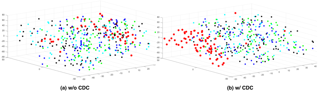
Features Visualization. Distribution of multi-level fused features for the testing videos on Protocol-1 OULU-NPU is shown in Fig. 8 via t-SNE maaten2008visualizing. It is clear that the features with CDC (Fig. 8(a)) presents more well-clustered behavior than that with vanilla convolution (Fig. 8(b)), which demonstrates the discrimination ability of CDC for distinguishing the living faces from spoofing faces. The visualization of the feature maps (w/o or w/ CDC) and attention maps of MAFM can be found in Appendix D.
5 Conclusions and Future Work
In this paper, we propose a novel operator called Central Difference Convolution (CDC) for face anti-spoofing task. Based on CDC, a Central Difference Convolutional Network (CDCN) is designed. We also propose CDCN++, consisting of a searched CDC backbone and Multiscale Attention Fusion Module (MAFM). Extensive experiments are performed to verify the effectiveness of the proposed methods. We note that the study of CDC is still at an early stage. Future directions include: 1) designing context-aware adaptive CDC for each layer/channel; 2) exploring other properties (e.g., domain generalization) and applicability on other vision tasks (e.g., image quality assessment ling2018role and FaceForensics).
6 Acknowledgment
This work was supported by the Academy of Finland for project MiGA (grant 316765), ICT 2023 project (grant 328115), and Infotech Oulu. As well, the authors wish to acknowledge CSC – IT Center for Science, Finland, for computational resources.
References
- (1) Martn Abadi, Paul Barham, Jianmin Chen, Zhifeng Chen, Andy Davis, Jeffrey Dean, Matthieu Devin, Sanjay Ghemawat, Geoffrey Irving, Michael Isard, et al. Tensorflow: a system for large-scale machine learning. In OSDI, volume 16, pages 265–283, 2016.
- (2) Timo Ahonen, Abdenour Hadid, and Matti Pietikainen. Face description with local binary patterns: Application to face recognition. IEEE Transactions on Pattern Analysis & Machine Intelligence, (12):2037–2041, 2006.
- (3) Shervin Rahimzadeh Arashloo, Josef Kittler, and William Christmas. An anomaly detection approach to face spoofing detection: A new formulation and evaluation protocol. IEEE Access, 5:13868–13882, 2017.
- (4) Yousef Atoum, Yaojie Liu, Amin Jourabloo, and Xiaoming Liu. Face anti-spoofing using patch and depth-based cnns. In 2017 IEEE International Joint Conference on Biometrics (IJCB), pages 319–328, 2017.
- (5) Samarth Bharadwaj, Tejas I Dhamecha, Mayank Vatsa, and Richa Singh. Computationally efficient face spoofing detection with motion magnification. In Proceedings of the IEEE conference on computer vision and pattern recognition workshops, pages 105–110, 2013.
- (6) Zinelabdine Boulkenafet, Jukka Komulainen, Zahid Akhtar, Azeddine Benlamoudi, Djamel Samai, Salah Eddine Bekhouche, Abdelkrim Ouafi, Fadi Dornaika, Abdelmalik Taleb-Ahmed, Le Qin, et al. A competition on generalized software-based face presentation attack detection in mobile scenarios. In 2017 IEEE International Joint Conference on Biometrics (IJCB), pages 688–696. IEEE, 2017.
- (7) Zinelabidine Boulkenafet, Jukka Komulainen, and Abdenour Hadid. Face anti-spoofing based on color texture analysis. In IEEE international conference on image processing (ICIP), pages 2636–2640, 2015.
- (8) Zinelabidine Boulkenafet, Jukka Komulainen, and Abdenour Hadid. Face spoofing detection using colour texture analysis. IEEE Transactions on Information Forensics and Security, 11(8):1818–1830, 2016.
- (9) Zinelabidine Boulkenafet, Jukka Komulainen, and Abdenour Hadid. Face antispoofing using speeded-up robust features and fisher vector encoding. IEEE Signal Processing Letters, 24(2):141–145, 2017.
- (10) Zinelabinde Boulkenafet, Jukka Komulainen, Lei Li, Xiaoyi Feng, and Abdenour Hadid. Oulu-npu: A mobile face presentation attack database with real-world variations. In FGR, pages 612–618, 2017.
- (11) Andrew Brock, Theodore Lim, James M Ritchie, and Nick Weston. Smash: one-shot model architecture search through hypernetworks. arXiv preprint arXiv:1708.05344, 2017.
- (12) Han Cai, Ligeng Zhu, and Song Han. Proxylessnas: Direct neural architecture search on target task and hardware. International Conference on Learning Representations (ICLR), 2019.
- (13) Ivana Chingovska, Andr Anjos, and Sbastien Marcel. On the effectiveness of local binary patterns in face anti-spoofing. In Biometrics Special Interest Group, pages 1–7, 2012.
- (14) Jifeng Dai, Haozhi Qi, Yuwen Xiong, Yi Li, Guodong Zhang, Han Hu, and Yichen Wei. Deformable convolutional networks. In Proceedings of the IEEE international conference on computer vision, pages 764–773, 2017.
- (15) Tiago de Freitas Pereira, Andr Anjos, Jos Mario De Martino, and Sbastien Marcel. Lbp- top based countermeasure against face spoofing attacks. In Asian Conference on Computer Vision, pages 121–132, 2012.
- (16) Tiago de Freitas Pereira, Andr Anjos, Jos Mario De Martino, and Sbastien Marcel. Can face anti-spoofing countermeasures work in a real world scenario? In 2013 international conference on biometrics (ICB), pages 1–8, 2013.
- (17) Xuanyi Dong and Yi Yang. Searching for a robust neural architecture in four gpu hours. In Proceedings of the IEEE Conference on Computer Vision and Pattern Recognition, pages 1761–1770, 2019.
- (18) Yao Feng, Fan Wu, Xiaohu Shao, Yanfeng Wang, and Xi Zhou. Joint 3d face reconstruction and dense alignment with position map regression network. In Proceedings of the European Conference on Computer Vision (ECCV), 2017.
- (19) Junying Gan, Shanlu Li, Yikui Zhai, and Chengyun Liu. 3d convolutional neural network based on face anti-spoofing. In ICMIP, pages 1–5, 2017.
- (20) Anjith George and Sébastien Marcel. Deep pixel-wise binary supervision for face presentation attack detection. In International Conference on Biometrics, number CONF, 2019.
- (21) Golnaz Ghiasi, Tsung-Yi Lin, and Quoc V Le. Nas-fpn: Learning scalable feature pyramid architecture for object detection. In Proceedings of the IEEE Conference on Computer Vision and Pattern Recognition, pages 7036–7045, 2019.
- (22) Kaiming He, Xiangyu Zhang, Shaoqing Ren, and Jian Sun. Deep residual learning for image recognition. In Proceedings of the IEEE conference on computer vision and pattern recognition, pages 770–778, 2016.
- (23) Gao Huang, Zhuang Liu, Laurens Van Der Maaten, and Kilian Q Weinberger. Densely connected convolutional networks. In Proceedings of the IEEE conference on computer vision and pattern recognition, pages 4700–4708, 2017.
- (24) international organization for standardization. Iso/iec jtc 1/sc 37 biometrics: Information technology biometric presentation attack detection part 1: Framework. In https://www.iso.org/obp/ui/iso, 2016.
- (25) Anil K Jain and Farshid Farrokhnia. Unsupervised texture segmentation using gabor filters. Pattern recognition, 24(12):1167–1186, 1991.
- (26) Amin Jourabloo, Yaojie Liu, and Xiaoming Liu. Face de-spoofing: Anti-spoofing via noise modeling. In Proceedings of the European Conference on Computer Vision (ECCV), pages 290–306, 2018.
- (27) Felix Juefei-Xu, Vishnu Naresh Boddeti, and Marios Savvides. Local binary convolutional neural networks. In Proceedings of the IEEE Conference on Computer Vision and Pattern Recognition, pages 19–28, 2017.
- (28) Jukka Komulainen, Abdenour Hadid, and Matti Pietikäinen. Face spoofing detection using dynamic texture. In Asian Conference on Computer Vision, pages 146–157. Springer, 2012.
- (29) Jukka Komulainen, Abdenour Hadid, and Matti Pietikainen. Context based face anti-spoofing. In 2013 IEEE Sixth International Conference on Biometrics: Theory, Applications and Systems (BTAS), pages 1–8, 2013.
- (30) Lei Li, Xiaoyi Feng, Zinelabidine Boulkenafet, Zhaoqiang Xia, Mingming Li, and Abdenour Hadid. An original face anti-spoofing approach using partial convolutional neural network. In IPTA, pages 1–6, 2016.
- (31) Xiaobai Li, Jukka Komulainen, Guoying Zhao, Pong-Chi Yuen, and Matti Pietikäinen. Generalized face anti-spoofing by detecting pulse from face videos. In 2016 23rd International Conference on Pattern Recognition (ICPR), pages 4244–4249. IEEE, 2016.
- (32) Bofan Lin, Xiaobai Li, Zitong Yu, and Guoying Zhao. Face liveness detection by rppg features and contextual patch-based cnn. In Proceedings of the 2019 3rd International Conference on Biometric Engineering and Applications, pages 61–68. ACM, 2019.
- (33) Chen Lin, Zhouyingcheng Liao, Peng Zhou, Jianguo Hu, and Bingbing Ni. Live face verification with multiple instantialized local homographic parameterization. In IJCAI, pages 814–820, 2018.
- (34) Suiyi Ling, Patrick Le Callet, and Zitong Yu. The role of structure and textural information in image utility and quality assessment tasks. Electronic Imaging, 2018(14):1–13, 2018.
- (35) Hanxiao Liu, Karen Simonyan, and Yiming Yang. Darts: Differentiable architecture search. International Conference on Learning Representations (ICLR), 2019.
- (36) Yaojie Liu, Amin Jourabloo, and Xiaoming Liu. Learning deep models for face anti-spoofing: Binary or auxiliary supervision. In Proceedings of the IEEE Conference on Computer Vision and Pattern Recognition, pages 389–398, 2018.
- (37) Yaojie Liu, Joel Stehouwer, Amin Jourabloo, and Xiaoming Liu. Deep tree learning for zero-shot face anti-spoofing. In Proceedings of the IEEE Conference on Computer Vision and Pattern Recognition, pages 4680–4689, 2019.
- (38) Shangzhen Luan, Chen Chen, Baochang Zhang, Jungong Han, and Jianzhuang Liu. Gabor convolutional networks. IEEE Transactions on Image Processing, 27(9):4357–4366, 2018.
- (39) Laurens van der Maaten and Geoffrey Hinton. Visualizing data using t-sne. Journal of machine learning research, 9(Nov):2579–2605, 2008.
- (40) Thomas J Palmeri and Isabel Gauthier. Visual object understanding. Nature Reviews Neuroscience, 5(4):291, 2004.
- (41) Gang Pan, Lin Sun, Zhaohui Wu, and Shihong Lao. Eyeblink-based anti-spoofing in face recognition from a generic webcamera. In IEEE International Conference on Computer Vision, pages 1–8, 2007.
- (42) Adam Paszke, Sam Gross, Soumith Chintala, Gregory Chanan, Edward Yang, Zachary DeVito, Zeming Lin, Alban Desmaison, Luca Antiga, and Adam Lerer. Automatic differentiation in pytorch. 2017.
- (43) Keyurkumar Patel, Hu Han, and Anil K Jain. Cross-database face antispoofing with robust feature representation. In Chinese Conference on Biometric Recognition, pages 611–619, 2016.
- (44) Keyurkumar Patel, Hu Han, and Anil K Jain. Secure face unlock: Spoof detection on smartphones. IEEE transactions on information forensics and security, 11(10):2268–2283, 2016.
- (45) Bruno Peixoto, Carolina Michelassi, and Anderson Rocha. Face liveness detection under bad illumination conditions. In ICIP, pages 3557–3560. IEEE, 2011.
- (46) Wei Peng, Xiaopeng Hong, and Guoying Zhao. Video action recognition via neural architecture searching. In 2019 IEEE International Conference on Image Processing (ICIP), pages 11–15. IEEE, 2019.
- (47) Hieu Pham, Melody Y Guan, Barret Zoph, Quoc V Le, and Jeff Dean. Efficient neural architecture search via parameter sharing. International Conference on Machine Learning (ICML), 2018.
- (48) Allan Pinto, Helio Pedrini, William Robson Schwartz, and Anderson Rocha. Face spoofing detection through visual codebooks of spectral temporal cubes. IEEE Transactions on Image Processing, 24(12):4726–4740, 2015.
- (49) Yunxiao Qin, Chenxu Zhao, Xiangyu Zhu, Zezheng Wang, Zitong Yu, Tianyu Fu, Feng Zhou, Jingping Shi, and Zhen Lei. Learning meta model for zero-and few-shot face anti-spoofing. AAAI, 2020.
- (50) Ruijie Quan, Xuanyi Dong, Yu Wu, Linchao Zhu, and Yi Yang. Auto-reid: Searching for a part-aware convnet for person re-identification. IEEE International Conference on Computer Vision, 2019.
- (51) Esteban Real, Alok Aggarwal, Yanping Huang, and Quoc V Le. Regularized evolution for image classifier architecture search. In Proceedings of the AAAI Conference on Artificial Intelligence, volume 33, pages 4780–4789, 2019.
- (52) Esteban Real, Sherry Moore, Andrew Selle, Saurabh Saxena, Yutaka Leon Suematsu, Jie Tan, Quoc V Le, and Alexey Kurakin. Large-scale evolution of image classifiers. In Proceedings of the 34th International Conference on Machine Learning-Volume 70, pages 2902–2911. JMLR. org, 2017.
- (53) Talha Ahmad Siddiqui, Samarth Bharadwaj, Tejas I Dhamecha, Akshay Agarwal, Mayank Vatsa, Richa Singh, and Nalini Ratha. Face anti-spoofing with multifeature videolet aggregation. In 2016 23rd International Conference on Pattern Recognition (ICPR), pages 1035–1040. IEEE, 2016.
- (54) Karen Simonyan and Andrew Zisserman. Very deep convolutional networks for large-scale image recognition. arXiv preprint arXiv:1409.1556, 2014.
- (55) Sabine Kastner Ungerleider and Leslie G. Mechanisms of visual attention in the human cortex. Annual review of neuroscience, 23(1):315–341, 2000.
- (56) Zezheng Wang, Chenxu Zhao, Yunxiao Qin, Qiusheng Zhou, and Zhen Lei. Exploiting temporal and depth information for multi-frame face anti-spoofing. arXiv preprint arXiv:1811.05118, 2018.
- (57) Di Wen, Hu Han, and Anil K Jain. Face spoof detection with image distortion analysis. IEEE Transactions on Information Forensics and Security, 10(4):746–761, 2015.
- (58) Sanghyun Woo, Jongchan Park, Joon-Young Lee, and In So Kweon. Cbam: Convolutional block attention module. In Proceedings of the European Conference on Computer Vision (ECCV), pages 3–19, 2018.
- (59) Fei Xiong and Wael AbdAlmageed. Unknown presentation attack detection with face rgb images. In 2018 IEEE 9th International Conference on Biometrics Theory, Applications and Systems (BTAS), pages 1–9. IEEE, 2018.
- (60) Yuhui Xu, Lingxi Xie, Xiaopeng Zhang, Xin Chen, Guo-Jun Qi, Qi Tian, and Hongkai Xiong. Pc-darts: Partial channel connections for memory-efficient differentiable architecture search. arXiv preprint arXiv:1907.05737, 2019.
- (61) Jianwei Yang, Zhen Lei, and Stan Z Li. Learn convolutional neural network for face anti-spoofing. arXiv preprint arXiv:1408.5601, 2014.
- (62) Xiao Yang, Wenhan Luo, Linchao Bao, Yuan Gao, Dihong Gong, Shibao Zheng, Zhifeng Li, and Wei Liu. Face anti-spoofing: Model matters, so does data. In Proceedings of the IEEE Conference on Computer Vision and Pattern Recognition, 2019.
- (63) Fisher Yu and Vladlen Koltun. Multi-scale context aggregation by dilated convolutions. arXiv preprint arXiv:1511.07122, 2015.
- (64) Zitong Yu, Yunxiao Qin, Xiaqing Xu, Chenxu Zhao, Zezheng Wang, Zhen Lei, and Guoying Zhao. Auto-fas: Searching lightweight networks for face anti-spoofing. ICASSP, 2020.
- (65) Yiheng Zhang, Zhaofan Qiu, Jingen Liu, Ting Yao, Dong Liu, and Tao Mei. Customizable architecture search for semantic segmentation. In Proceedings of the IEEE Conference on Computer Vision and Pattern Recognition, pages 11641–11650, 2019.
- (66) Zhiwei Zhang, Junjie Yan, Sifei Liu, Zhen Lei, Dong Yi, and Stan Z Li. A face antispoofing database with diverse attacks. In ICB, pages 26–31, 2012.
- (67) Ning Zhu and Xiaolong Bai. Neural architecture search for deep face recognition. arXiv preprint arXiv:1904.09523, 2019.
- (68) Barret Zoph and Quoc V Le. Neural architecture search with reinforcement learning. International Conference on Learning Representations (ICLR), 2017.
- (69) Barret Zoph, Vijay Vasudevan, Jonathon Shlens, and Quoc V Le. Learning transferable architectures for scalable image recognition. In Proceedings of the IEEE conference on computer vision and pattern recognition, pages 8697–8710, 2018.
Appendix
A. Derivation and Code of CDC
Here we show the detailed derivation (Eq.(4) in draft) of CDC in Eq. (7) and Pytorch code of CDC in Fig. 9.
| (7) |
B. Adaptive for CDC
Although the best hyperparameter can be manually measured for face anti-spoofing task, it is still troublesome to find the best-suited when applying Central Difference Convolution (CDC) to other datasets/tasks. Here we treat as the data-driven learnable weights for each layer. A simple implementation is to utilize to guarantee the output range within .
As illustrated in Fig. 10(a), it is interesting to find that the values of learned weights in low (2nd to 4th layer) and high (8th to 10th layer) levels are relatively small while that in mid (5th to 7th layer) level are large. It indicates that the central difference gradient information might be more important for mid level features. In terms of the performance comparison, it can be seen from Fig. 10(b) that adaptive CDC achieves comparable results (1.8% vs. 1.0% ACER) with CDC using constant .

| Method | Metrics(%) | Replay | Mask Attacks | Makeup Attacks | Partial Attacks | Average | |||||||||||||||
|
|
|
|
|
|
|
|
|
|
| |||||||||||
| SVMRBF+LBP Boulkenafet2017OULU | APCER | 19.1 | 15.4 | 40.8 | 20.3 | 70.3 | 0.0 | 4.6 | 96.9 | 35.3 | 11.3 | 53.3 | 58.5 | 0.6 | 32.829.8 | ||||||
| BPCER | 22.1 | 21.5 | 21.9 | 21.4 | 20.7 | 23.1 | 22.9 | 21.7 | 12.5 | 22.2 | 18.4 | 20.0 | 22.9 | 21.02.9 | |||||||
| ACER | 20.6 | 18.4 | 31.3 | 21.4 | 45.5 | 11.6 | 13.8 | 59.3 | 23.9 | 16.7 | 35.9 | 39.2 | 11.7 | 26.914.5 | |||||||
| EER | 20.8 | 18.6 | 36.3 | 21.4 | 37.2 | 7.5 | 14.1 | 51.2 | 19.8 | 16.1 | 34.4 | 33.0 | 7.9 | 24.512.9 | |||||||
| Auxiliary Liu2018Learning | APCER | 23.7 | 7.3 | 27.7 | 18.2 | 97.8 | 8.3 | 16.2 | 100.0 | 18.0 | 16.3 | 91.8 | 72.2 | 0.4 | 38.337.4 | ||||||
| BPCER | 10.1 | 6.5 | 10.9 | 11.6 | 6.2 | 7.8 | 9.3 | 11.6 | 9.3 | 7.1 | 6.2 | 8.8 | 10.3 | 8.9 2.0 | |||||||
| ACER | 16.8 | 6.9 | 19.3 | 14.9 | 52.1 | 8.0 | 12.8 | 55.8 | 13.7 | 11.7 | 49.0 | 40.5 | 5.3 | 23.618.5 | |||||||
| EER | 14.0 | 4.3 | 11.6 | 12.4 | 24.6 | 7.8 | 10.0 | 72.3 | 10.1 | 9.4 | 21.4 | 18.6 | 4.0 | 17.017.7 | |||||||
| DTN liu2019deep | APCER | 1.0 | 0.0 | 0.7 | 24.5 | 58.6 | 0.5 | 3.8 | 73.2 | 13.2 | 12.4 | 17.0 | 17.0 | 0.2 | 17.123.3 | ||||||
| BPCER | 18.6 | 11.9 | 29.3 | 12.8 | 13.4 | 8.5 | 23.0 | 11.5 | 9.6 | 16.0 | 21.5 | 22.6 | 16.8 | 16.6 6.2 | |||||||
| ACER | 9.8 | 6.0 | 15.0 | 18.7 | 36.0 | 4.5 | 7.7 | 48.1 | 11.4 | 14.2 | 19.3 | 19.8 | 8.5 | 16.8 11.1 | |||||||
| EER | 10.0 | 2.1 | 14.4 | 18.6 | 26.5 | 5.7 | 9.6 | 50.2 | 10.1 | 13.2 | 19.8 | 20.5 | 8.8 | 16.1 12.2 | |||||||
| CDCN (Ours) | APCER | 8.2 | 6.9 | 8.3 | 7.4 | 20.5 | 5.9 | 5.0 | 43.5 | 1.6 | 14.0 | 24.5 | 18.3 | 1.2 | 12.711.7 | ||||||
| BPCER | 9.3 | 8.5 | 13.9 | 10.9 | 21.0 | 3.1 | 7.0 | 45.0 | 2.3 | 16.2 | 26.4 | 20.9 | 5.4 | 14.6 11.7 | |||||||
| ACER | 8.7 | 7.7 | 11.1 | 9.1 | 20.7 | 4.5 | 5.9 | 44.2 | 2.0 | 15.1 | 25.4 | 19.6 | 3.3 | 13.6 11.7 | |||||||
| EER | 8.2 | 7.8 | 8.3 | 7.4 | 20.5 | 5.9 | 5.0 | 47.8 | 1.6 | 14.0 | 24.5 | 18.3 | 1.1 | 13.1 12.6 | |||||||
| CDCN++ (Ours) | APCER | 9.2 | 6.0 | 4.2 | 7.4 | 18.2 | 0.0 | 5.0 | 39.1 | 0.0 | 14.0 | 23.3 | 14.3 | 0.0 | 10.811.2 | ||||||
| BPCER | 12.4 | 8.5 | 14.0 | 13.2 | 19.4 | 7.0 | 6.2 | 45.0 | 1.6 | 14.0 | 24.8 | 20.9 | 3.9 | 14.611.4 | |||||||
| ACER | 10.8 | 7.3 | 9.1 | 10.3 | 18.8 | 3.5 | 5.6 | 42.1 | 0.8 | 14.0 | 24.0 | 17.6 | 1.9 | 12.711.2 | |||||||
| EER | 9.2 | 5.6 | 4.2 | 11.1 | 19.3 | 5.9 | 5.0 | 43.5 | 0.0 | 14.0 | 23.3 | 14.3 | 0.0 | 11.911.8 | |||||||
C. Cross-type Testing on SiW-M
Following the same cross-type testing protocol (13 attacks leave-one-out) on SiW-M dataset liu2019deep, we compare our proposed methods with three recent face anti-spoofing methods Boulkenafet2017OULU; Liu2018Learning; liu2019deep to valid the generalization capacity of unseen attacks. As shown in Table 8, our CDCN++ achieves an overall better ACER and EER, with the improvement of previous state-of-the-art liu2019deep by 24% and 26% respectively. Specifically, we detect almost all ”Impersonation” and ”Partial Paper” attacks (EER=0%) while the previous methods perform poorly on ”Impersonation” attack. It is obvious that we reduce the both the EER and ACER of Mask attacks (”HalfMask”, ”SiliconeMask”, ”TransparentMask” and ”MannequinHead”) sharply, which shows our CDC based methods generalize well on 3D nonplanar attacks.
D. Feature Visualization
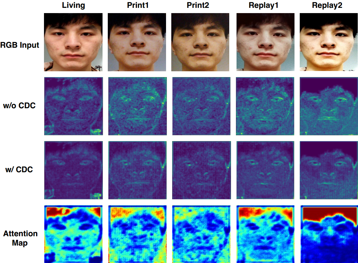
The low-level features and corresponding spatial attention maps of MAFM are visualized in Fig. 11. It is clear that both the features and attention maps between living and spoofing faces are quite different. 1) For the low-level features (see 2nd and 3rd row in Fig. 11), neural activation from the spoofing faces seems to be more homogeneous between the facial and background regions than that from living faces. It’s worth noting that features with CDC are more likely to capture the detailed spoofing patterns (e.g., lattice artifacts in ”Print1” and reflection artifacts in ”Replay2”). 2) For the spatial attention maps of MAFM (see 4th row in Fig. 11), all the regions of hair, face and background have the relatively strong activation for the living faces while the facial regions contribute weakly for the spoofing faces.