August 11, 2026
Deep learning for passive source detection in presence of complex cargo
Abstract
Methods for source detection in high noise environments are important for single-photon emission computed tomography (SPECT) medical imaging and especially crucial for homeland security applications, which is our main interest. In the latter case, one deals with passively detecting the presence of low emission nuclear sources with significant background noise (with Signal To Noise Ratio () or less). In passive emission problems, direction sensitive detectors are needed, to match the dimensionalities of the image and the data. Collimation, used for that purpose in standard Anger -cameras, is not an option. Instead, Compton -cameras (and their analogs for other types of radiation) can be utilized. Backprojection methods suggested before by two of the authors and their collaborators enable detection in the presence of a random uniform background. In most practical applications, however, cargo packing in shipping containers and trucks creates regions of strong absorption and scattering, while leaving some streaming gaps open. In such cases backprojection methods prove ineffective and lose their detection ability. Nonetheless, visual perception of the backprojection pictures suggested that some indications of presence of a source might still be in the data. To learn such features (if they do exist), a deep neural network approach is implemented in 2D, which indeed exhibits higher sensitivity and specificity than the backprojection techniques in a low scattering case and works well when presence of complex cargo makes backprojection fail completely.
Keywords:
source detection, Compton camera, illicit nuclear material1 Introduction
Checking for presence of illicit nuclear materials (most probably in small quantities and shielded by cargo) at border crossings and shipping cargo containers in harbors is an important homeland security task. Ideally, one would try to reconstruct from the detected signals the source distribution inside the cargo. When the data is sufficiently well behaved (e.g., in SPECT), analytic reconstruction is often possible [27]. However, in a very low SNR environment, as in the case of illicit nuclear source detection, this is impossible. Indeed, the forward analytic (integral transform type) models are not applicable. Moreover, even if they were, attempts of any filtration in FBP-type techniques lead to disaster. The saving grace is that in this case practitioners are mostly interested in getting reliable (i.e., with low rates of false positives and false negatives) information about the presence of a source, rather than its exact location.
As is well known, in passive emission imaging detectors must be direction sensitive. Indeed, otherwise the data measured has insufficient dimension for recovery of an image. Directional information is especially critical when SNR is too low for the intensity fluctuations that arise due to the presence of a source to be statistically significant. The following options for obtaining directional sensitivity are available:
- •
Mechanical collimation, when only rays incident along (or close to) a certain line are allowed to reach the detector (see Section 2). This, while determining the incoming photon’s direction, significantly reduces the signal strength and thus becomes unsuitable for low SNR.
- •
Compton -cameras represent a more recent, and gaining its appreciation, type of radiation detectors that determine a surface cone of possible incident trajectories, rather than the exact directions.
- •
Neutron detectors are being developed that (albeit based on different physics principles) produce similar cone information and lead to similar mathematical analysis.
Backprojection detection technique introduced in [5, 30] relied upon finding suspicious locations. It utilized the following three assumptions:
- 1.
geometric smallness of the source (usually of linear dimension on the order of of the linear cargo size);
- 2.
existence of a sufficient number of particles from the source reaching the detector being ballistic (non-scattered);
- 3.
unstructured strong random background.
The idea is very simple: backprojecting the incoming trajectories (or, in the Compton case, the whole surface cones of possible trajectories) of particles, one hopes that maybe, due to sufficient presence of ballistic particles detected from the source, one can see a statistically significant accumulation at the geometrically small source’s location (see Fig. 1)
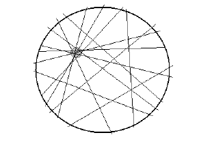
Analysis done in [5] provided a crude formula for the total number of particles (and thus observation time) needed to make detection with high (on the order of ) sensitivity and specificity (i.e., with low levels of false negatives and false positives).
| (1) |
Here is the ratio of the linear dimension of the source relative to the dimension of the cargo and is the SNR, defined as the proportion of the ballistic particles from the source versus the total number of source and background particles. In the cases considered in [5] had to be on the order of , which is not unrealistic for photons not screened by heavily shielding cargo. High specificity has been hardwired into the method, so satisfying (1) was only needed in [5, 6] to ensure high sensitivity.
The implementation of the technique worked as follows [5, 6]: the data was backprojected, which resulted in a large background level throughout the volume. When the object was completely surrounded by detectors, this level was essentially constant and the mean was removed. When the detectors did not surround the object completely (e.g., no detector below the object), the global mean is irrelevant, and at each location the mean over a smaller patch was removed. After this clean-up the locations with an intensity less than five standard deviations above the mean suggested by the Central Limit Theorem were cut off. The results were interpreted as indications of a source being present. Thousands of Monte Carlo simulations showed that the inequality (1) agrees well with experiments and if is at or above this threshold, detection occurs with high sensitivity and specificity 11 1 An alternative Bayesian approach was implemented in [30]..
This technique works reasonably well in the absence of complex cargo, but starts failing if such cargo is present [6], due to the second and third assumptions being inapplicable22 2 This cargo problem is mostly non-existent when detecting neutrons coming from the source. However, some other (non-mathematical) issues arise, such as for instance lower number of particles detected.. However, visual inspection of the backprojected data (see [6]) seems to indicate that the data might still contain a signature of the source presence. Indeed, when the method of [5] was applied to some cases of complex cargo in [6], despite its failure to detect presence of the source, such signatures (e.g., different highlighting of the pathways between cargo boxes) seemed to appear only when a source was present (see Figure 2). The reader should take into account that the color scales are different in the three pictures there and assigned automatically by the visualization software. This is of no importance, since it is not the intensity, but rather the patterns of highlighted pathways between boxes seem different.
 |
 |
 |
No model of this effect has been developed, no telling features have been learned, and thus no detection algorithm came out of such observations.
This has led the authors to attempt deep learning for the source inference in the hope that a network could learn what we could not. Thus, our main goal is to detect the presence/absence of a source, not necessarily its location. If there is high probability of presence of the source, in practice one would check the cargo with other (hand-held) devices. However, one also needs to achieve high specificity, to avoid large numbers of false positives.
We describe now the structure of the article. Section 2 contains a brief description of the Compton type cameras and references to the known analytic approaches. Success of deploying neural networks is predicated upon our access to sufficient data for neural network training. Thus, the first step - generating various complex cargo scenarios is described in Section 3. To avoid the inverse crime (overfitting), different processes of generating cargos are used for creating training and testing samples. Then, in absence of real data (which would require having weapons grade nuclear materials and physically creating thousands of different cargoes), we use (Section 4) the technique of forward radiation transport simulations customarily used in nuclear engineering. As has been mentioned, the actual type of radiation is mathematically irrelevant, but to be close to real world scenarios and numerical parameter values, the case of -photons coming from an U-238 source and real world material parameters for cargo are used. The design of the network is described in section 5. The results are presented in Section 6. Additional remarks can be found in section 7. Acknowledgements are provided in section 8. Some auxiliary tables, figures, and algorithm descriptions are located in the Appendix.
2 Collimated and Compton -Cameras
Mechanical collimators (see Figure 3) can be installed in front of a direction insensitive camera to block all particles but those incident along (or close to) a desired trajectory.
 |
 |
Mechanical collimators are widely used in medical imaging. They, however, significantly attenuate the signal and require rotating the detector (or the object). In the applications with sufficiently high , this additional data loss is not such a problem. In dealing with low signals however, this renders recovery of weak signals impossible. For this reason one can consider Compton type cameras instead.
The Compton camera is a type of -particle detector33 3 As we have mentioned before, novel neutron detectors (albeit based upon different physics rather than Compton scattering) that provide mostly similar cone information are currently being developed. that does not attenuate the incident particles. The price to pay is that it provides less precise direction information than collimation would give. Namely, only a surface cone of possible incoming directions is measured rather than a precise trajectory (see Fig 4).

In the absence of mechanical collimation, signal strength is effectively maintained, although the directional information is less precise and thus data analysis becomes more complex. On the other hand, the data provided is significantly over-determined (e.g., the space of cones in is five-dimensional, versus the unknown distribution being three-dimensional). This turns out not to be a bad thing at all, but rather a blessing for stable inversion (see [27] for details and further references).
A variety of exact inversion formulas from Compton data of filtered-backprojection and other types have been developed and implemented (see [27] and references therein). The choices are much more diverse than for the usual Radon transform inversions (see [22]). The reason is that the Compton data is highly overdetermined. It was shown that this feature can be used to get high quality reconstructions in SPECT in presence of % noise and higher. However, this is a far cry from the low SNRs encountered in the homeland security problems described above.
3 Simulating Cargo Scenarios
If one intends to tackle a problem using deep learning, it is natural to start by acquiring large amounts of training and testing data.
In order to obtain rich training data for a neural network, at least thousands (better hundreds of thousands or millions) of cargo configurations are needed. The more training data can be obtained, the better. Due to the sensitive nature of the materials involved in this work, we are unable to procure real-world data, so we resort to synthetic simulation. The high computation costs of these simulations restricted us to several thousands of samples, reaching up to . However, our results (see Section 6) already show a success in detection.
To start, we randomly produce several thousand cargo configurations and compute forward radiation data simulations with up to four randomly placed sources and without them for each one. In order to avoid overfitting (and an inverse crime), different cargo generation procedures are used for producing the training and testing data.
3.1 Procedural Generation of Training Cargo Configurations
A square cargo hold of size of is assumed and partitioned into cells (the possible source would occupy one of them). Each cell can be indexed via a pair of row and column indices, , with and is assigned a material identification number . These numbers correspond to a variety of materials, including Air, concrete, highly enriched uranium, iron, cotton, wood, plastic, and fertilized (their detailed chemical content described in [6]).
Real cargo typically consists of several boxes with small spaces in between. In order to emulate this, an algorithm is implemented to generate different cargo configurations. It consists of three main steps:
- •
A network of several horizontal and vertical “corridors” between boxes with random widths and locations is generated. The number of corridors is selected randomly in a desired range .
- •
The resulting configurations are unlikely to be symmetric, while real cargo might happen to be symmetric. To check whether symmetry plays any role in detectability44 4 Disclosure: Our results show that symmetries do not influence detectability., a portion of the samples produced are “symmetrized” by enforcing various (rotation and mirror) symmetry rules.
- •
Connected components of the rest of the space are identified as distinct “cargo boxes.” Then material contents are assigned to all boxes. In a subset of (rather than all) symmetric cargo configurations, material contents are also “symmetrized” according to the corresponding rule.
Generating the corridors between pieces of cargo is performed using a modification of the procedure outlined in [9] for generating road networks. For the training set, we only use networks consisting of horizontal and vertical segments, while for the testing set tilted and non-orthogonal pathways are allowed.
Remark.
Instead of selecting corridor locations uniformly randomly, their locations for training are selected according to a probability distribution generated from a type of gradient noise developed in [23] in order to automate the production of realistic looking textures in computer graphics. A different algorithm is used for testing samples.
Identification of connected components (“boxes”) is performed using SciPy’s (Scientific Python, a popular Python package for scientific computing [15]) implementation of the algorithms outlined in [29].
The entire generation procedure is summarized in Algorithm 1 in the Appendix (Section 9).
 |
 |
 |
 |
 |
 |
 |
 |
 |
 |
3.2 Procedural Generation of Testing Cargo Configurations
To avoid the inverse crime of overfitting, testing configurations are produced by a somewhat similar, but independent algorithm. Namely, the middle points, the lengths and width of the corridors are selected randomly and independently. Moreover, the corridors are not required to be vertical or horizontal, or even orthogonal at their intersections anymore. Finding the boxes (connected components of the complement) and filling them with materials is also done randomly, similarly to the training case.
3.3 Source placement
A source of a (randomized) strength corresponding to approximately SNR is placed randomly into the cargo.
Multiple sources (, or ) are also modeled to see the effect on detection. Two scenarios are used:
- 1.
when all the sources have the same strength SNR
and - 2.
when the strength of the source is diluted between several locations.
One naturally expects deterioration of the detection in the 2nd case, while a priori it would not be surprising if it happened in the 1st as well (although our results will demonstrate that this does not happen). Indeed, the backprojection detection, as well most probably the one by deep networks, if successful, should use some geometric assumptions (e.g., geometric smallness of the source), since the source’s strength alone would not be statistically significant. Thus, multiplying the number of sources in principle might degrade the geometric features of importance (albeit one does not know what these are).
4 Forward radiation simulations
As previously mentioned, the nature of particles is irrelevant, but in order to be in realistic situations, the particle detection is considered, where the material parameters and emission and background rates that are used assume realistic values.
After the cargo scenario has been created, one needs to simulate training and testing data by solving a massive forward radiation transport computation. Luckily, this is what nuclear engineering researchers are trained to do.
4.1 Physics Preliminary
U-238 (Uranium-238) photons from the 1.001 MeV emission line have mean-free-path in high-Z materials sufficiently high to be detected outside the container (13.3mm mean-free-paths) [26]. In our application, sources of background radiation include a concrete base located some distance below the container. (Cosmic rays and other natural sources can be easily included and do not influence the results much.) These background sources radiate at much higher energies than 1.001 MeV, including 1.461 MeV from Potassium-40, 1.12 MeV and 1.76 MeV from Bismuth-214, and 2.61 MeV from Thallium-208 (Bismuth and Thallium are products of the decay of Uranium-238 and Thorium 232 respectively, and are present in trace amounts in concrete). Gamma photons which downscatter from these sources into the energy group surrounding the 1.001 MeV line account for the noise in our signal. Gamma photons from the source will also undergo scattering and absorption within the volume of the container, which will reduce the number of ballistic source particles reaching the detectors placed around the container, thus weakening the signal.
4.2 Mathematics of the forward radiation data simulation
The radiation transport within the cargo container is modeled by the linear Boltzmann equation, given below using the multigroup approximation:
| (2) |
where is the position, the set of discrete directions and the energy group. is the volume of the cargo container, is the unit sphere, is the total number of energy groups, is the photon angular flux in the energy group , is the total interaction cross section in group , is the Legendre moment of the scattering cross section from group to group , is the maximum anisotropy expansion order, and is the volumetric source of photons in group (stemming from the U-238 source). The moments of the angular flux are given by
| (3) |
where is the spherical harmonic of order of and degree . Eq. (2) is supplied with boundary conditions:
| (4) |
where is the incoming boundary defined as with the outward unit normal vector at position . The function describes the background radiation due to a large concrete slab underneath the container, as previously described. Cross sections for various materials were generated using NJOY-99 [21]. The multigroup structure employed ranges from MeV to MeV with narrow bands centered at the radiation lines of the background and U-238.
For the purposes of this paper, calculations are carried out in two-dimensional space and only the energy group corresponding to the 1.001 MeV line is considered after solving Eq. (2). The photon transport equation, Eq. (2), is discretized using standard techniques:
- 1.
product Gauss-Legendre-Tchebychev angular quadrature [25] is employed (only a small number of polar angles are needed, but a very high number of azimuthal angles are needed to resolve properly the angular distribution in the 2D domain.)
- 2.
- 3.
Transport sweeps and Source Iteration are employed to solve the resulting system. [19]
Once the transport equation (2) has been solved, the outgoing angular photon flux at any boundary edge in 2D is recorded, which serves as the input data for use in Deep Learning and Backprojection.
Once configurations have been generated, a radiating source emitting an expected photons per second at MeV is randomly placed, a forward radiative transfer equation is solved, and from its solution the radiation angular flux distribution on the boundary of the cargo is collected.
Due to linearity of (2), the situations of presence of zero to four randomly placed sources could (and were) easily incorporated.
5 Convolutional Neural Network
Using a fully connected network for the problem seems to be hardly feasible even in 2D, less so in 3D, in particular due to high dimensionality of the Compton camera data. The saving grace here is that, as in many imaging problems [20], one expects that the important correlations occur mostly between close pixels, and hence convolutional neural networks, which are much more compact due to weight sharing, offer a hope. We thus construct, train, and test a deep convolutional neural network (CNN). This hand-waving argument for using CNN needs to be confirmed by computations, which is done in this text.
The suggested CNN architecture is summarized in Figure 6 below. The input data dimension is , as we model 400 equally spaced detectors with 360 equally spaced angular bins and only one energy bin is used. The network is trained on unique simulated cargo configurations with varying numbers of sources present. By exploiting the fact that the Boltzmann equation (2) is linear, we can produce multiple new samples from each configuration by taking varying combinations of sources and detectors. We simulate up to four sources per configuration, and four linear arrays of detectors along each edge of the cargo. This leads to a total of total samples. The various combinations are summarized in Table 1 Below.
| Number of Sources | One Detector | Two Adjacent Detectors | Two Opposite Detectors | Three Detectors | Four Detectors | Total |
|---|---|---|---|---|---|---|
| 0 | 6756 | 6756 | 3378 | 6756 | 1689 | 25335 |
| 1 | 27024 | 27024 | 13512 | 27024 | 6756 | 101340 |
| 2 | 40536 | 40536 | 20268 | 40536 | 10134 | 152010 |
| 3 | 27024 | 27024 | 13512 | 27024 | 6756 | 101340 |
| 4 | 6756 | 6756 | 3378 | 6756 | 1689 | 25335 |
| Total | 108096 | 108096 | 54048 | 108096 | 27024 | 405360 |
The output of the CNN is two probability measures: on and on . A source is determined to be present if , and absent otherwise. predicts the number of sources present, which we set to . The loss function used for training is the binary cross-entropy loss:
| (5) |
where is the network prediction and is the target value (see [13]). The CNN was trained on simulations of a localized source in the presence of high background noise (). In all cases, early stopping is used to halt training before over-fitting. The various hyper-parameter values used in training are summarized in Table 2 below. The CNN is implemented using Keras with Tensorflow as its backend. Keras is a high level API (Application Programming Interface) for interfacing with machine learning toolkits such as Tensorflow, Theano, and Microsoft Cognitive Toolkit. It helps streamline the construction and training of neural networks [10]. Tensorflow is Google’s machine learning toolkit and was chosen due to its scalability, wide range of features, and the wide range of documentation and tutorials available [1]. Any parameters not explicitly mentioned here were set to default values.

| Optimization Method | Adam (See [16]) |
|---|---|
| Activation | RELU (Softmax at output) |
| Bias | True |
| Convolution Window Size | 3x3 |
| Learning Rate | |
| Learning Rate Decay Rate | 0 |
| Batch Size | 4 |
| Early Stopping Patience | 3 epochs |
| Loss | Binary Cross-Entropy |
6 Results
After training the CNN, we considered a large variety of cargo scenarios to test and to compare and contrast the performance of the CNN against the backprojection method of [5, 6]. We detail some interesting specific example scenarios in Sections 6.1 and 6.2. We then investigate the statistical performance of the CNN on large scale data sets to evaluate the sensitivity and specificity of the CNN in Section 6.3, and to assess its performance with different numbers of sources and detectors in Section 6.4. Finally, in Section 6.5 we discuss the relation between cargo configuration and exposure time and how this affects the practicality of our technique.
6.1 Example Scenarios
We describe now several (out of many, see later on in this text) sample results of testing the trained network on various scenarios not included in the training set.
6.1.1
Example #1
This configuration (right) as well as backprojection (left) with source present is shown in Figure 7 below. The backprojection procedure described in the Introduction did not lead to any statistically significant detection. We, however, show the raw (not cleaned up) backprojection picture for the reader to notice the corridor highlighting phenomenon observed in [6]. The network, on the other hand, succeeds in detecting presence of the source. This is one of the heavy iron configurations which has a shorter exposure time (18 seconds for 101,180 background particles).
 |
 |
6.1.2
Example #2
Next we consider the scenario shown in Figure 8, where backprojection fails to detect the source (and thus is not shown), but the network succeeds. Here the exposure time needed for the detection is significantly longer. In this configuration a long thick iron slab effectively blocks one side of the detectors. Smaller chunks of iron spread throughout the container further attenuate the signal along certain trajectories. As a result, it would take 9 hours and 26 minutes to detect the needed 101,092 particles. Unless one is talking about a shipping container, this is practically unfeasible. As the results in Section 6.3 show, twice shorter time would still do decently, and even five times shorter time might sometimes be used, although at the expense of higher false positive rate.
 |
6.1.3
Example #3
Here we consider a somewhat more tenable scenario shown in Figure 9, where backprojection fails to detect the source, yet the network succeeds. In this case the exposure time is 50 minutes and 17 seconds for 100,866 particles. In this configuration several large blocks of iron are periodically tiled in the container, with the source located within one of the blocks.
 |
6.1.4
Example #4
Now we consider a somewhat extreme scenario (Figure 10), where both approaches succeed in detecting the source. In this case the exposure time is 3 days and 12 hours for collecting 101,272 particles. In this configuration one very large block of iron in the center of the container surrounds the source. The source is still localized relatively well by backprojection for this scenario. Most of the cargo is filled with a homogeneous material, which might explain why backprojection did not fail.
 |
 |
6.1.5
Example #5
Next, we consider a rather easy scenario (Figure 11), where both backprojection and the network succeed. In this case the exposure time is 276 milliseconds for 100,898 particles. In this configuration several small blocks of different materials are spread throughout the container. Only an insignificant amount of particles are scattered, so backprojection recovers the source distribution extremely well.
 |
 |
6.2 Generalization to more complex scenarios
Now we will include more complex situations, significantly different from the ones used for training. Namely, the corridors are not necessarily aligned vertically and horizontally, nor are intersecting corridors orthogonal. The algorithm of producing configurations was different from the one used in training. Additionally, we allow multiple sources to be present. The results show that the network passes well this generalization test.
6.2.1
Example #6
In this configuration (see Figure 12) several iron blocks are spread throughout the container, but a sufficient amount of low attenuating paths exist between the sources and detector arrays for backprojection to recover the sources well. There are two sources present very near to each other. This clearly aids the backprojection method in successfully detecting the sources. The CNN also succeeds in detecting presence of both of the sources. Here the exposure time is 649 milliseconds for 101,497 particles.
 |
 |
6.2.2
Example #7
In this configuration (Figure 13) several heavy iron blocks cut diagonally through the container slightly off-center. Three sources are present in this scenario, the two sources around the middle are localized well with backprojection, since most of the materials only weakly attenuate the signal, but the source on the other side of the heavy iron has several attenuating materials to contend with, so the backprojection smears its signature throughout the diagonal corridor it’s in. Both backprojection and the CNN successfully predict that there is a source, although backprojection fails to locate the third source. This third source may prove difficult for the CNN to contend with as well, as the CNN predicts there are only two sources present. Here the exposure time is 371 milliseconds for 102,790 particles.
 |
 |
6.2.3
Example #8
Here several iron blocks surround the center of the container (Figure 14). Four sources are present in this scenario, two of them directly adjacent (and thus hard to distinguish in the picture) and all four are near the center of the container. In this case backprojection fails to localize any of the sources due the limited angular information in the signal as a result of the attenuating properties of the iron. The CNN, on the other hand succeeds in detecting the presence of all four of the sources, even despite the close proximity of two of them. Here the exposure time is 1.97 seconds for 103,789 particles.
 |
6.2.4
Example #9
Finally, we consider a simple case where backprojection and the CNN both succeed. In this case there is ample angular information for backprojection to localize the source well and the CNN correctly predicts the presence of a single source. The exposure time is 21.92 seconds for 100,672 particles. The configuration can be seen in Figure 15 below.
 |
 |
6.3 Performance on Large Scale Dataset
To test the statistical performance of the CNN on a large scale, unique cargo configurations are generated using an alternate (to avoid possible inverse crime) generative scheme. For each cargo configuration all four linear detector arrays are present, from zero up to four sources are randomly placed and simulated independently, so that by using linearity of (2) we can produce testing samples. Particle detections are simulated for an exposure time measured by the expected background detection levels of , and particles. The data were fed into the trained CNN for source presence detection. The results for presence detection are summarized in Table 3 below. The results obtained clearly confirm our expectations (see Section 1).
| Expected Particle Count | Sensitivity | Specificity |
|---|---|---|
| 100000 | 99.90% | 99.71% |
| 50000 | 99.78% | 94.59% |
| 20000 | 99.81% | 36.36% |
For comparison, the backprojection showed in the case of around particles sensitivity of about with high specificity (as we have mentioned, the high specificity was built into the backprojection method). In the case of particles, the sensitivity drops to .
We remind the reader that sensitivity, or true positive rate, shows the success of determining the presence of a source (i.e., few false negatives), while specificity reflects how well the absence of the source is detected (i.e., few false positives). High specificity was hardwired into the BP techniques [5, 6], it was only the sensitivity that was questionable.
The accuracy of the prediction generally increases with particle count (and thus observation time), and sufficient particle counts are required for successful detection. At the low levels (e.g., of 20000 particles and lower) the network seems biased to think that a source is always present. This clearly leads to near sensitivity and an extremely low specificity, which makes the detection practically not feasible, due to high level of false positives.. An explanation could be that the features that are being detected (albeit we do not know what they are) are non-smooth, vs. large smooth background. When the total count is low, the whole dataset becomes non-smooth, which tricks the network.
For particles CNN succeeds extremely well and, as is mentioned above, beats hands down the backprojection technique, which often does not show any statistically significant deviations and thus does not detect presence of the source. Notice that six times higher number of detected particles was required in [5, 30] for stable detection, even without complex cargo being involved. This makes any application of backprojection technique to complex cargo situation groundless and unreliable (even though in almost cases, some of which we already have presented, the location of the source is detected).
6.4 Number of sources and number of detector arrays
Here we address the question of whether one has to completely surround the object with four detectors, or some results can be achieved with three, two, or one flat detector arrays. We thus have simulated each cargo configuration with zero to four independent sources randomly placed. Just as with the training data, we take several combinations of which sources and detector arrays are present. The combinations are summarized in Table 4 below.
| Number of Sources | One Detector | Two Adjacent Detectors | Two Opposite Detectors | Three Detectors | Four Detectors | Total |
|---|---|---|---|---|---|---|
| 0 | 6952 | 6952 | 3476 | 6952 | 1738 | 26070 |
| 1 | 27808 | 27808 | 13904 | 27808 | 6952 | 104280 |
| 2 | 41712 | 41712 | 20856 | 41712 | 10428 | 156420 |
| 3 | 27808 | 27808 | 13904 | 27808 | 6952 | 104280 |
| 4 | 6952 | 6952 | 3476 | 6952 | 1738 | 26070 |
| Total | 111232 | 111232 | 55616 | 111232 | 27808 | 417120 |
Particle detections are simulated for an exposure time measured by the expected background detection levels of , and particles. The data were fed into the trained CNN for inference. The results for presence detection are summarized in Tables 6, 7 and 8 and the results for source number prediction are summarized in Tables 9, 10 and 11, all in Section 9.
Additionally, we investigated the effect of scaling the strength of each source so that altogether they had the same strength as a single source, thus effectively diluting the localized signature of the source. In the case of backprojection the localized nature of the source is the key justification for the method of [5]. This would lead one to believe that splitting the source strength will make it more difficult for the CNN to detect any source presence, which is indeed confirmed by the results summarized in Table 5 below.
| Expected Particle Count | Sensitivity one source | Sensitivity two sources | Sensitivity three sources | Sensitivity four sources | Specificity |
|---|---|---|---|---|---|
| 100000 | 99.74% | 96.57% | 89.67% | 82.62% | 99.71% |
| 50000 | 99.68% | 97.25% | 93.51% | 89.13% | 94.59% |
| 20000 | 99.99% | 99.95% | 99.86% | 99.77% | 36.36% |
6.5 Observation time
The above results are presented in terms of the total number of particles detected. The conclusion is natural: the larger - the better. The number of detected particles obviously increases with (essentially proportional to) the time of observation. However, the slope of this increase clearly depends significantly on the type and configuration of the cargo. Thus, the exposure time required to reach a certain level of particle detections is a function of the configuration of the cargo, including source location, material composition, material placement, and background strength. This makes it difficult to predict boundary flux rates, even if the configuration is known, without solving the Boltzmann equation (2).
To make a fair numerical experiment, many heavily iron (and thus very shielding) cargo scenarios have been included. Namely, the set of all samples have been divided into 24 sets of equal size, and the probability of choosing iron as the filling of boxes was increasing linearly from zero in the first group to almost one in the 24th one. Figure 16 contains the histogram of the number of runs vs. time required for detection for thousands of configuration runs for detecting the presence of a source emitting on the order of 1000 particles (assuming four detectors). The vast majority would require time measured in seconds.
Generally speaking, one would epect the large bin on the left-hand side to correspond to configurations with less high-Z materials, and the larger bins on the right-hand side correspond to configurations with more high-Z materials. It can certainly become unrealistic to detect many source particles in some of the latter cases. Nevertheless, as is evidenced by some of the examples presented, as well as statistics presented in Section 6.3, quite a few configurations of high-Z material exist where presence of source(s) source can be detected in a reasonable amount of time. These lower exposure time scenarios would be the most appropriate cases for detecting illicit nuclear materials at border crossings. Some of the longer exposure times (on the order of several minutes to perhaps several days) would be appropriate for detection of illicit nuclear materials in shipping containers on cargo ships, where scanning can be done while the container is in transit.
Additionally, it is important to note that if one restricts oneself to a smaller number of detector arrays (incomplete view), it will take longer to reach the same exposure level and thus would add to the number of undetected cases.
7 Remarks and Conclusions
- •
Our work shows that the deep learning approach significantly improves over detection by backprojection techniques of [27, 6, 30] and works for complex attenuating and scattering cargo scenarios, where the latter fails completely. This confirms the opinion expressed in [6] that some information about source presence was there.
- •
- •
The network performs well detecting the number of up to four sources (although naturally somewhat less successfully than detecting mere presence of a source).
- •
The authors want to make clear that when producing the results of this paper, no processing (e.g., backprojecting) of the raw detector data is done before feeding it to the network. Since the authors do not know what features would be of importance, we have decided to not impose our prejudices on the data (especially taking into account that backprojection is a smoothing operator, and the relevant information is most probably contained in some sharper features).
- •
The exposure time required for detection is discussed in Section 6.5. The histogram in Figure 16 shows detection in a matter of second for a vast majority of configurations.
It is clear that there are some unbeatable shieldings, so one cannot aim for the success rate. In such cases, other detection techniques could be used: from methods of detecting presence of significant amounts of (shielding) high-Z materials, to neutron emission detection, to human intelligence.
- •
A strong effort has been made to avoid committing an inverse crime. The testing samples have been produced by an algorithm independent of the one used for the training data. The testing cargo geometries were different from the ones not encountered in the training data, so there was no intersection between the two data-sets.
- •
A variety of symmetry rules, including rotational symmetry and mirror symmetry were applied randomly to some of the configurations and their material content, to check whether presence or absence of the symmetry influence the detectability. The network performance does not seem to react to this.
- •
The reader should not think that retraining was needed for different tasks and situations, e.g. for heavy iron cargo, or for detecting the number of sources, rather their mere presence. This all was done with a single trained network.
- •
Four planar Compton detectors forming a square surrounding the object of interrogation were assumed. It seems that this is the most practical design of such detectors. Effects of removal of some of the detectors have also been studied (Section 6.4).
The rectangular shape causes some problems, though, e.g. in backprojection method they create (easily removable) corner artifacts. More importantly, this design lacks full rotational invariance, which could be beneficial for the NN design. On the other hand, the rectangular case is challenged by appearance of tilted cargo structures in the test samples, while they were absent in the training data. The network, however, clearly has overcome this difficulty.
- •
There are various further improvements that one should attempt (and are being attempted). Some of them are addressed below.
- 1.
It would have been great to figure out what specifically were the signs of presence of the source that the network has learned. This would open a door for developing more analytic methods. However, at this moment the authors do not know what these features are.
- 2.
Producing many more training data is a serious stumbling block in 2D, and especially in 3D case.
- 3.
The CNN architecture should be improved, aiming to reach shorter observation time and even lower SNR levels.
- 4.
We are working on moving to the more realistic 3D situation. The significant difference here is, first, the much higher dimensionality of the data (5D) and corresponding much more massive computations that are needed. Second, in 3D, unlike 2D (where a cone consists just of two rays), the Compton data differ significantly from the usual Radon ones. In particular, an issue arises of how to bin the five-dimensional Compton data in such a way, that the use of CNN could be warranted.
- 5.
The neural network (NN) approach should be tested on real data, which the authors clearly do not have. However, the radiative transport forward computations we used are commonly practiced in nuclear engineering, seem to be very realistic, and involve realistic material parameters. There is a chance that when novel neutron detectors that are being developed are deployed, we could get some real data.
- 6.
The approach we describe indicates presence of a source, but not its location (at least in the heavy iron cargo case). One wonders whether location can also be attempted.
- 7.
Although the results presented have been obtained by the same once trained NN, during research various designs of the NN and training sets have been experimented with, all showing consistent ability of detection. It would be still important to study further the model uncertainty (e.g., by using the dropout technique [12]). This will be done in a future work.
Meanwhile, although the testing samples often deviated from the structures used in the training set, our results have shown that the NN generalized extremely well. High experimental levels of the sensitivity and specificity, as well as more detailed information presented in Section 6.3 about statistical spread of the results instill confidence in the suitability of the network as a detection tool.
The imperfection of Compton camera detections has been partially addressed by randomizing the source strength and location and finite bin sizes for the detected data. Depending on the quality of the future detectors, the bin sizes might have to be increased and new study conducted.
- 8.
When source particles scatter they lose energy. If source particles downscatter to lower energy groups we will lose them in our data since we only use the highest energy group. It would be interesting to try and use these lower energy groups in either a 3D convolution with 1 channel or a 2D convolution with multiple channels to see if we can get better results.
- 1.
8 Acknowledgements
The first two authors acknowledge the support from the National Science Foundation through the DMS grant #1816430 and Texas A&M Cyclotron Institute. The third author has been partially supported through a grant by the Department of the Defense, Defense Threat Reduction Agency under Award No. HDTRA1-18-1-0020. The content of the article does not necessarily reflect the position or the policy of the federal government, and no official endorsement should be inferred.
The authors are truly indebted to the three referees, whose detailed comments served not only to improve exposition, but even more importantly, attracted our attention to some features we have missed.
References
References
- [1] Abadi M, et. al. 2015 Tensorflow: Large-Scale Machine Learning on Heterogeneous Systems https://www.tensorflow.org/
- [2] Adams M P, Adams M L, Hawkins W D, Smith T, Rauchwerger L, Amato N M, Bailey T S and Falgout R D 2013 Provably optimal parallel transport sweeps on regular grids International Conference on Mathematics and Computational Methods Applied to Nucl. Sci. & Eng. 4 2535
- [3] Adams M P, Adams M L, McGraw C N and Till A T 2015 Provably optimal parallel transport sweeps with non-contiguous partitions ANS MC2015-Joint International Conference on Mathematics and Computation (M&C), Supercomputing in Nuclear Applications (SNA) and the Monte Carlo (MC) Method 2 1218
- [4] Adams M P, Adams M L, Hawkins W D, Smith T, Rauchwerger L, Amato N M, Bailey T S, Falgout R D, Kunen A and Brown P 2020 Provably optimal parallel transport sweeps on semi-structured grids Journal of Computational Physics 01/2020 109234
- [5] Allmaras M, Darrow D, Hristova Y, Kanschat G and Kuchment P 2010 Detecting small low emission radiating sources Inverse Problems & Imaging, 7(1) 47
- [6] Allmaras M, Ciabatti A, Hristova Y, Kuchment P, Olson A and Ragusa J 2016 Passive Detection of Small Low-Emission Sources: Two-Dimensional Numerical Case Studies Nuclear Sci. and Eng. 184(1) 125
- [7] Bell G I and Glasstone S 1970 Nuclear reactor theory. (Malabar, FL: Krieger Publishing Company)
- [8] Carlson B G 1955 Solutions of the Transport Equation by SN Approximations (Los Alamos, NM: Los Alamos Scientific Laboratory)
- [9] Chen G, Esch G, Wonka P, Müller P and Zhang E 2008 Interactive Procedural Street Modeling ACM Trans. Graph. 27 1
- [10] Chollet F 2015 Keras GitHub https://github.com/fchollet/keras
- [11] Duderstadt J J and Martin W R 1979 Transport theory (New York, NY: John Wiley & Sons)
- [12] Y. Gal, Z. Ghahramani, Dropout as a Bayesian approcimation: representing model uncertainty in deep learning, Proceedings of the 33rd International Conference on Machine Learning, New York, NY, USA, 2016. JMLR: W&CP volume 48.
- [13] Goodfellow I, Bengio Y and Courville A 2016 Deep Learning (Cambridge, MA: MIT Press)
- [14] Hawkins W D, Bailey T S, Adams M L, Brown P N, Kunen A J, Adams M P, Smith T, Amato N M and Rauchwerger L 2014 Validation of Full-Domain Massively Parallel Transport Sweep Algorithms Trans. Amer. Nucl. Soc. 111 699
- [15] Jones E, et. al. 2001 SciPy: Open Source Scientific Tools for Python http://www.scipy.org/
- [16] Kingma D P and Ba J 2015 Adam: A Method for Stochastic Optimization International Conference on Learning Representations
- [17] Lamarsh J 1966 Introduction to nuclear reactor theory. (Boston, MA: Addison-Wesley series in nuclear engineering. Addison-Wesley Pub. Co.)
- [18] Lesaint P and Raviart P A 1974 On a finite element method for solving the neutron transport equation. Mathematical Aspects of Finite Elements in Partial Differential Equations, 33 89
- [19] Lewis E E and Miller W F 1984 Computational methods of neutron transport (United States: John Wiley and Sons, Inc.)
- [20] Liu W, Wang Z, Liu X, Zeng N, Liu Y and Alsaadi F 2017 A survey of deep neural network architectures and their applications, Neurocomputing 234 11
- [21] MacFarlane R and Muir D 1994 The NJOY nuclear data processing system version 91 (Los Alamos, NM: Los Alamos Scientific Laboratory)
- [22] Natterer F 2001 Mathematics of computerized tomography (Philadelphia, PA: SIAM: Society for Industrial and Applied Mathematics)
- [23] Perlin K 1985 An Image Synthesizer Proceedings of the 12th Annual Conference on Computer Graphics and Interactive Techniques 10 287
- [24] Reed W H and Hill T R 1973 Triangular mesh methods for the neutron transport equation. National topical meeting on mathematical models and computational techniques for analysis of nuclear systems Los Alamos Report LA-UR-73-479
- [25] Sánchez R and Ragusa J 2011 On the construction of galerkin angular quadratures Nuclear Science and Engineering 169(2) 133
- [26] Santi P A 2013 Passive nondestructive assay of nuclear materials (Los Alamos NM: Los Alamos Scientific Laboratory) Los Alamos Report LA-UR-73-479
- [27] Terzioglu F, Kuchment P and Kunyansky L 2018 Compton camera imaging and the cone transform : A brief overview Inverse Problems 34(5) 054002.
- [28] Wareing T, McGhee J, Morel J and Pautz S 2001 Discontinuous finite element Sn methods on three-dimensional unstructured grids Nuclear Science and Engineering, 138(3) 256
- [29] Wu K, Otoo E and Shoshani A 2005 Optimizing connected component labeling algorithms Medical Imaging 2005: Image Processing 5747 1965
- [30] Xun X, Mallick B, Carroll R and Kuchment P 2011 Bayesian approach to detection of small low emission sources Inverse Problems 27(11) 115009
9 Appendix
9.1 Algorithm for Procedural Generation of Cargo Configurations
9.2 Statistics of the source(s) detection
| Number of Sources | CNN Prediction | |
|---|---|---|
| Source Present | No Source Present | |
| 0 | 6.04 % | 93.36 % |
| 1 | 98.35 % | 1.65 % |
| 2 | 99.90 % | 0.10 % |
| 3 | 99.98 % | 0.02 % |
| 4 | 100.00 % | 0.00 % |
| Number of Sources | CNN Prediction | |
|---|---|---|
| Source Present | No Source Present | |
| 0 | 3.31 % | 96.69 % |
| 1 | 99.20 % | 0.80 % |
| 2 | 99.96 % | 0.04 % |
| 3 | 100.00 % | 0.00 % |
| 4 | 100.00 % | 0.00 % |
| Number of Sources | CNN Prediction | |
|---|---|---|
| Source Present | No Source Present | |
| 0 | 1.41 % | 98.59 % |
| 1 | 99.15 % | 0.85 % |
| 2 | 99.96 % | 0.04 % |
| 3 | 100.00 % | 0.00 % |
| 4 | 100.00 % | 0.00 % |
| Number of Sources | CNN Prediction | |
|---|---|---|
| Source Present | No Source Present | |
| 0 | 0.55 % | 99.45 % |
| 1 | 99.19 % | 0.81 % |
| 2 | 99.97 % | 0.03 % |
| 3 | 99.99 % | 0.01 % |
| 4 | 99.99 % | 0.01 % |
| Number of Sources | CNN Prediction | |
|---|---|---|
| Source Present | No Source Present | |
| 0 | 0.29 % | 99.71 % |
| 1 | 99.27 % | 0.73 % |
| 2 | 100.00 % | 0.00 % |
| 3 | 100.00 % | 0.00 % |
| 4 | 100.00 % | 0.00 % |
| Number of Sources | CNN Prediction | |
|---|---|---|
| Source Present | No Source Present | |
| 0 | 2.85 % | 97.15 % |
| 1 | 98.97 % | 1.03 % |
| 2 | 99.95 % | 0.05 % |
| 3 | 99.99 % | 0.01 % |
| 4 | 100.00 % | 0.00 % |
| Number of Sources | CNN Prediction | |
|---|---|---|
| Source Present | No Source Present | |
| 0 | 15.03 % | 84.97 % |
| 1 | 97.51 % | 2.49 % |
| 2 | 99.76 % | 0.24 % |
| 3 | 99.98 % | 0.02 % |
| 4 | 100.00 % | 0.00 % |
| Number of Sources | CNN Prediction | |
|---|---|---|
| Source Present | No Source Present | |
| 0 | 11.39 % | 88.81 % |
| 1 | 98.86 % | 1.14 % |
| 2 | 99.93 % | 0.07 % |
| 3 | 100.00 % | 0.00 % |
| 4 | 100.00 % | 0.00 % |
| Number of Sources | CNN Prediction | |
|---|---|---|
| Source Present | No Source Present | |
| 0 | 7.91 % | 92.09 % |
| 1 | 99.04 % | 0.96 % |
| 2 | 99.95 % | 0.05 % |
| 3 | 99.99 % | 0.01 % |
| 4 | 100.00 % | 0.00 % |
| Number of Sources | CNN Prediction | |
|---|---|---|
| Source Present | No Source Present | |
| 0 | 6.67 % | 93.33 % |
| 1 | 99.12 % | 0.87 % |
| 2 | 99.96 % | 0.04 % |
| 3 | 99.99 % | 0.01 % |
| 4 | 99.99 % | 0.01 % |
| Number of Sources | CNN Prediction | |
|---|---|---|
| Source Present | No Source Present | |
| 0 | 5.41 % | 94.59 % |
| 1 | 99.18 % | 0.82 % |
| 2 | 99.99 % | 0.01 % |
| 3 | 100.00 % | 0.00 % |
| 4 | 100.00 % | 0.00 % |
| Number of Sources | CNN Prediction | |
|---|---|---|
| Source Present | No Source Present | |
| 0 | 10.24 % | 89.76 % |
| 1 | 98.62 % | 1.38 % |
| 2 | 99.90 % | 0.10 % |
| 3 | 99.99 % | 0.01 % |
| 4 | 100.00 % | 0.00 % |
| Number of Sources | CNN Prediction | |
|---|---|---|
| Source Present | No Source Present | |
| 0 | 66.59 % | 33.41 % |
| 1 | 97.77 % | 2.23 % |
| 2 | 99.57 % | 0.43 % |
| 3 | 99.90 % | 0.10 % |
| 4 | 100.00 % | 0.00 % |
| Number of Sources | CNN Prediction | |
|---|---|---|
| Source Present | No Source Present | |
| 0 | 66.20 % | 33.80 % |
| 1 | 98.90 % | 1.10 % |
| 2 | 99.86 % | 0.14 % |
| 3 | 99.99 % | 0.01 % |
| 4 | 100.00 % | 0.00 % |
| Number of Sources | CNN Prediction | |
|---|---|---|
| Source Present | No Source Present | |
| 0 | 64.79 % | 35.21 % |
| 1 | 99.17 % | 0.83 % |
| 2 | 99.91 % | 0.09 % |
| 3 | 99.95 % | 0.05 % |
| 4 | 100.00 % | 0.00 % |
| Number of Sources | CNN Prediction | |
|---|---|---|
| Source Present | No Source Present | |
| 0 | 62.87 % | 37.13 % |
| 1 | 99.32 % | 0.68 % |
| 2 | 99.94 % | 0.06 % |
| 3 | 99.99 % | 0.01 % |
| 4 | 99.99 % | 0.01 % |
| Number of Sources | CNN Prediction | |
|---|---|---|
| Source Present | No Source Present | |
| 0 | 63.64 % | 36.36 % |
| 1 | 99.34 % | 0.66 % |
| 2 | 99.99 % | 0.01 % |
| 3 | 100.00 % | 0.00 % |
| 4 | 100.00 % | 0.00 % |
| Number of Sources | CNN Prediction | |
|---|---|---|
| Source Present | No Source Present | |
| 0 | 65.06 % | 34.94 % |
| 1 | 98.77 % | 1.23 % |
| 2 | 99.82 % | 0.18 % |
| 3 | 99.96 % | 0.04 % |
| 4 | 100.00 % | 0.00 % |
| No. Sources | CNN Prediction | ||||
|---|---|---|---|---|---|
| 0 | 1 | 2 | 3 | 4 | |
| 0 | 94.88 % | 3.90 % | 0.81 % | 0.27 % | 0.14 % |
| 1 | 1.73 % | 76.00 % | 20.05 % | 1.87 % | 0.35 % |
| 2 | 0.11 % | 6.93 % | 71.89 % | 20.04 % | 1.03 % |
| 3 | 0.01 % | 0.54 % | 22.46 % | 71.03 % | 5.96 % |
| 4 | 0.00 % | 0.06 % | 4.00 % | 62.62 % | 33.32 % |
| No. Sources | CNN Prediction | ||||
|---|---|---|---|---|---|
| 0 | 1 | 2 | 3 | 4 | |
| 0 | 97.41 % | 2.29 % | 0.26 % | 0.04 % | 0.00 % |
| 1 | 0.88 % | 78.80 % | 19.75 % | 0.55 % | 0.02 % |
| 2 | 0.05 % | 4.41 % | 76.05 % | 19.38 % | 0.11 % |
| 3 | 0.00 % | 0.33 % | 17.19 % | 77.73 % | 4.75 % |
| 4 | 0.00 % | 0.10 % | 2.11 % | 59.74 % | 38.05 % |
| No. Sources | CNN Prediction | ||||
|---|---|---|---|---|---|
| 0 | 1 | 2 | 3 | 4 | |
| 0 | 98.85 % | 1.04 % | 0.12 % | 0.00 % | 0.00 % |
| 1 | 0.87 % | 80.48 % | 18.46 % | 0.19 % | 0.00 % |
| 2 | 0.04 % | 4.38 % | 76.09 % | 19.41 % | 0.08 % |
| 3 | 0.00 % | 0.40 % | 15.94 % | 78.41 % | 5.25 % |
| 4 | 0.00 % | 0.06 % | 2.68 % | 58.03 % | 39.24 % |
| No. Sources | CNN Prediction | ||||
|---|---|---|---|---|---|
| 0 | 1 | 2 | 3 | 4 | |
| 0 | 99.73 % | 0.26 % | 0.01 % | 0.00 % | 0.00 % |
| 1 | 0.82 % | 79.06 % | 20.06 % | 0.07 % | 0.00 % |
| 2 | 0.03 % | 3.62 % | 75.65 % | 20.61 % | 0.09 % |
| 3 | 0.01 % | 0.37 % | 15.09 % | 78.96 % | 5.57 % |
| 4 | 0.01 % | 0.14 % | 2.20 % | 57.95 % | 39.69 % |
| No. Sources | CNN Prediction | ||||
|---|---|---|---|---|---|
| 0 | 1 | 2 | 3 | 4 | |
| 0 | 99.83 % | 0.17 % | 0.00 % | 0.00 % | 0.00 % |
| 1 | 0.76 % | 78.91 % | 20.24 % | 0.09 % | 0.00 % |
| 2 | 0.00 % | 3.10 % | 75.84 % | 20.94 % | 0.12 % |
| 3 | 0.00 % | 0.13 % | 11.84 % | 82.39 % | 5.64 % |
| 4 | 0.00 % | 0.00 % | 1.27 % | 58.63 % | 40.10 % |
| No. Sources | CNN Prediction | ||||
|---|---|---|---|---|---|
| 0 | 1 | 2 | 3 | 4 | |
| 0 | 97.71 % | 1.87 % | 0.30 % | 0.08 % | 0.04 % |
| 1 | 1.08 % | 78.36 % | 19.77 % | 0.70 % | 0.10 % |
| 2 | 0.05 % | 4.78 % | 74.83 % | 19.99 % | 0.35 % |
| 3 | 0.01 % | 0.39 % | 17.51 % | 76.67 % | 5.42 % |
| 4 | 0.00 % | 0.09 % | 2.66 % | 59.73 % | 37.52 % |
| No. Sources | CNN Prediction | ||||
|---|---|---|---|---|---|
| 0 | 1 | 2 | 3 | 4 | |
| 0 | 86.12 % | 12.15 % | 1.18 % | 0.40 % | 0.14 % |
| 1 | 2.40 % | 78.08 % | 17.33 % | 1.82 % | 0.37 % |
| 2 | 0.22 % | 14.08 % | 72.57 % | 12.27 % | 0.87 % |
| 3 | 0.03 % | 1.52 % | 39.20 % | 56.29 % | 2.96 % |
| 4 | 0.00 % | 0.24 % | 9.34 % | 74.58 % | 15.84 % |
| No. Sources | CNN Prediction | ||||
|---|---|---|---|---|---|
| 0 | 1 | 2 | 3 | 4 | |
| 0 | 90.51 % | 9.06 % | 0.33 % | 0.10 % | 0.00 % |
| 1 | 1.17 % | 79.42 % | 18.87 % | 0.54 % | 0.01 % |
| 2 | 0.07 % | 8.50 % | 78.92 % | 12.42 % | 0.09 % |
| 3 | 0.00 % | 0.82 % | 31.23 % | 66.29 % | 1.65 % |
| 4 | 0.00 % | 0.13 % | 5.51 % | 76.14 % | 18.22 % |
| No. Sources | CNN Prediction | ||||
|---|---|---|---|---|---|
| 0 | 1 | 2 | 3 | 4 | |
| 0 | 93.70 % | 6.16 % | 0.12 % | 0.03 % | 0.00 % |
| 1 | 0.93 % | 79.93 % | 18.95 % | 0.19 % | 0.00 % |
| 2 | 0.05 % | 7.29 % | 80.41 % | 12.21 % | 0.03 % |
| 3 | 0.00 % | 0.75 % | 26.55 % | 71.14 % | 1.56 % |
| 4 | 0.00 % | 0.12 % | 5.18 % | 73.48 % | 21.23 % |
| No. Sources | CNN Prediction | ||||
|---|---|---|---|---|---|
| 0 | 1 | 2 | 3 | 4 | |
| 0 | 95.17 % | 4.80 % | 0.03 % | 0.00 % | 0.00 % |
| 1 | 0.88 % | 78.23 % | 20.81 % | 0.07 % | 0.00 % |
| 2 | 0.05 % | 5.52 % | 79.87 % | 14.54 % | 0.02 % |
| 3 | 0.02 % | 0.49 % | 24.45 % | 72.89 % | 2.15 % |
| 4 | 0.03 % | 0.16 % | 4.03 % | 73.22 % | 32.57 % |
| No. Sources | CNN Prediction | ||||
|---|---|---|---|---|---|
| 0 | 1 | 2 | 3 | 4 | |
| 0 | 96.26 % | 3.74 % | 0.00 % | 0.00 % | 0.00 % |
| 1 | 0.82 % | 78.45 % | 20.66 % | 0.07 % | 0.00 % |
| 2 | 0.01 % | 4.46 % | 81.02 % | 14.46 % | 0.05 % |
| 3 | 0.00 % | 0.16 % | 20.71 % | 76.68 % | 2.45 % |
| 4 | 0.00 % | 0.00 % | 2.13 % | 76.35 % | 21.52 % |
| No. Sources | CNN Prediction | ||||
|---|---|---|---|---|---|
| 0 | 1 | 2 | 3 | 4 | |
| 0 | 91.39 % | 8.01 % | 0.43 % | 0.14 % | 0.04 % |
| 1 | 1.37 % | 78.75 % | 19.11 % | 0.68 % | 0.10 % |
| 2 | 0.10 % | 8.76 % | 77.82 % | 13.05 % | 0.27 % |
| 3 | 0.01 % | 0.87 % | 30.22 % | 66.72 % | 2.17 % |
| 4 | 0.01 % | 0.16 % | 5.86 % | 74.60 % | 19.37 % |
| No. Sources | CNN Prediction | ||||
|---|---|---|---|---|---|
| 0 | 1 | 2 | 3 | 4 | |
| 0 | 31.21 % | 61.87 % | 5.37 % | 1.29 % | 0.26 % |
| 1 | 1.88 % | 60.02 % | 34.37 % | 3.19 % | 0.53 % |
| 2 | 0.36 % | 15.92 % | 69.30 % | 13.38 % | 1.04 % |
| 3 | 0.10 % | 3.15 % | 49.37 % | 44.95 % | 2.43 % |
| 4 | 0.00 % | 0.70 % | 19.63 % | 71.29 % | 8.37 % |
| No. Sources | CNN Prediction | ||||
|---|---|---|---|---|---|
| 0 | 1 | 2 | 3 | 4 | |
| 0 | 32.05 % | 64.82 % | 2.88 % | 0.26 % | 0.00 % |
| 1 | 1.02 % | 57.93 % | 39.83 % | 1.19 % | 0.03 % |
| 2 | 0.12 % | 9.84 % | 76.55 % | 13.36 % | 0.12 % |
| 3 | 0.01 % | 1.63 % | 41.18 % | 56.22 % | 0.96 % |
| 4 | 0.00 % | 0.35 % | 12.07 % | 79.67 % | 7.91 % |
| No. Sources | CNN Prediction | ||||
|---|---|---|---|---|---|
| 0 | 1 | 2 | 3 | 4 | |
| 0 | 34.00 % | 64.44 % | 1.44 % | 0.09 % | 0.03 % |
| 1 | 0.81 % | 57.32 % | 41.28 % | 0.58 % | 0.01 % |
| 2 | 0.10 % | 7.88 % | 78.02 % | 13.92 % | 0.09 % |
| 3 | 0.05 % | 1.22 % | 35.99 % | 61.92 % | 0.81 % |
| 4 | 0.00 % | 0.17 % | 10.47 % | 80.58 % | 8.77 % |
| No. Sources | CNN Prediction | ||||
|---|---|---|---|---|---|
| 0 | 1 | 2 | 3 | 4 | |
| 0 | 35.87 % | 63.64 % | 0.45 % | 0.04 % | 0.00 % |
| 1 | 0.65 % | 54.57 % | 44.47 % | 0.31 % | 0.00 % |
| 2 | 0.05 % | 6.00 % | 78.01 % | 15.93 % | 0.02 % |
| 3 | 0.01 % | 0.70 % | 32.67 % | 65.65 % | 0.96 % |
| 4 | 0.03 % | 0.17 % | 7.72 % | 82.65 % | 9.42 % |
| No. Sources | CNN Prediction | ||||
|---|---|---|---|---|---|
| 0 | 1 | 2 | 3 | 4 | |
| 0 | 35.85 % | 63.98 % | 0.17 % | 0.00 % | 0.00 % |
| 1 | 0.66 % | 55.64 % | 43.33 % | 0.37 % | 0.00 % |
| 2 | 0.00 % | 4.66 % | 79.39 % | 15.93 % | 0.02 % |
| 3 | 0.00 % | 0.32 % | 29.59 % | 68.83 % | 1.27 % |
| 4 | 0.00 % | 0.00 % | 4.60 % | 84.58 % | 10.82 % |
| No. Sources | CNN Prediction | ||||
|---|---|---|---|---|---|
| 0 | 1 | 2 | 3 | 4 | |
| 0 | 33.36 % | 63.61 % | 2.52 % | 0.44 % | 0.07 % |
| 1 | 1.10 % | 57.36 % | 40.04 % | 1.35 % | 0.15 % |
| 2 | 0.15 % | 9.83 % | 75.39 % | 14.30 % | 0.33 % |
| 3 | 0.04 % | 1.65 % | 39.63 % | 57.33 % | 1.35 % |
| 4 | 0.01 % | 0.35 % | 12.22 % | 78.68 % | 8.75 % |