Adaptive Extremum Seeking Using Recursive Least Squares

Consider a concave static map system

$\displaystyle y=h_{s}(u)=\bar{h}_{s}(\theta^{*},u),\quad\theta^{*}=\begin{bmatrix}\theta^{*}_{1}&\cdots&\theta^{*}_{N}\end{bmatrix}^{T},$

(1)

where $\theta^{*}\in\mathbb{R}^{N}$ is a fixed unknown parameter vector, $u\in\mathbb{R}^{m}$ is the input and $y\in\mathbb{R}$ is the output of the system. Assume that the control input signal $u$ is generated by a smooth control law

$$u=\alpha(\theta)$$

(2)

parametrized by a control parameter vector $\theta\in\mathbb{R}^{N}$.

The control objective is to maximize the steady-state value of $y$ but without requiring the knowledge of $\theta^{*}$ or the system function $h_{s}$.

Consider a general multi-input-single-output (MISO) nonlinear system

$$\dot{x}=f(x,u)=\bar{f}(\theta^{*},x,u),$$

(3)

$$y=h_{d}(x)=\bar{h}_{d}(\theta^{*},\theta)=h(\theta),$$

(4)

$$\theta=\pi(x)$$

(5)

where $x\in\mathbb{R}^{n}$ is the state, $u\in\mathbb{R}^{m}$ is the input, $y\in\mathbb{R}$ is the output, all measurable, and $f:\mathbb{R}^{n}\times\mathbb{R}^{m}\rightarrow\mathbb{R}^{n}$ and $h_{d}=h\circ\pi$ are smooth functions. Assume that the control input signal $u$ is in the form (2), the control parameter $\theta\in\mathbb{R}^{N}$ is dependant on $x$ through a map $\pi(.):\mathbb{R}^{n}\rightarrow\mathbb{R}^{N}$.

The closed loop system can be written as follows:

$$\dot{x}=f(x,\alpha(\theta))=f(x,\alpha(\pi(x)).$$

(6)

The equilibria of (6) can be parameterized by $\theta$. The following assumptions about the closed loop system (3) are made, similarly to [21].

The control objective is to maximize the steady-state value of $y$ but without requiring the knowledge of $\theta^{*}$ or the system functions $h_{d},f$. This objective could be perfectly performed if $\theta^{*}$ was known and substituted in (2).

The control parameter vector estimation can be done in different ways, leading to different ES schemes, even for the fixed control structure (2). The assumption that $h$ has a maximum is without loss of generality, considering a maximum seeking task. Minimum seeking case would be treated identically, replacing $y$ with $-y$ in the subsequent feedback design.

In the next section, existing classical perturbation based ES approach will be reviewed to give an idea about our proposed design and to later use in simulation comparisons.

Consider the static map (1) and the control law (2) for scalar case, $N=1$, under Assumptions 1 and 2 about the closed-loop system. The proposed scheme is depicted in Fig. 2.

RLS estimation based ES block shown in Fig. 2 consists of two parts: an RLS based adaptive parameter identifier estimating the gradient $h_{\theta}=\frac{\partial y}{\partial\theta}$ and a control law to be fed by this estimate.

Consider the static map equation (1). In this equation, the time derivative of the output $y$ is given by

$$\dot{y}=h_{\theta}\dot{\theta}.$$

(12)

Design of the RLS based estimator to generate $\hat{h}_{\theta}$ considers the relation (12) that is in the linear parametric model form.

$$z=h_{\theta}\phi.$$

(13)

where

$$z=\dot{y},\quad\phi=\dot{\theta}.$$

(14)

If $\dot{y}$ is not available for measurement, then the regressor signals can be generated as

$\displaystyle z=\frac{s}{s+\omega_{l}}[y],\quad\phi=\frac{1}{s+\omega_{l}}[\dot{\theta}],$

(15)

i.e.,

$\displaystyle\dot{z}=-\omega_{l}z+\dot{y},\quad\dot{\phi}=-\phi\omega_{l}+\dot{\theta},$

(16)

where $\omega_{l}>0$ is a constant design parameter. The control law generating $\theta$ is proposed to be

$$\dot{\theta}=k\hat{h}_{\theta},\quad k>0.$$

(17)

Assuming that the time variation of $h_{\theta}$ is sufficiently slow, we design an RLS estimator for the parametric model (13) as follows:

$$\dot{\hat{h}}_{\theta}=p\epsilon\phi,$$

(18)

$$\dot{p}=\beta p-p^{2}\phi^{2},$$

(19)

$$\epsilon=z-\hat{h}_{\theta}\phi,$$

(20)

where $\beta>0$ is forgetting factor and $p$ is the covariance term. The overall ES scheme producing $\theta(t)$ can be summarized by (17), (18), (19), and (20).

The RLS estimation based ES control scheme (17)-(20) applies to the dynamic system (3)-(5) for $N=1$ with the control law (2) under Assumptions 3 and 4. The proposed ES scheme is depicted in Fig. 3.

In this section, stability proof of the proposed schemes in Sections IV-A and IV-B will be presented. We know that $\theta^{*}$ is the equilibrium point and the estimated gradient will be $h_{\theta}=0$ at the equilibrium point $\theta=\theta^{*}$. We can write our stability result as follows:

Consider the block diagram in Fig. 4 for the static map in (1). The time derivative of (1) is given by

$$\dot{y}=h_{\theta}^{T}\dot{\theta},$$

(24)

which, similarly to (13), can be written in the linear parametric form

$$z=h_{\theta}^{T}\phi,$$

(25)

where $z$ and $\phi$ are again defined by either (14) or (15). The control law (17) is used for updating $\theta$ in the vector case as well. The design of the RLS estimator to produce $\hat{h}_{\theta}$ is based on the parametric model (25) and is given as follows ([25]):

$$\dot{\hat{h}}_{\theta}=P\epsilon\phi,$$

(26)

$$\dot{P}=\beta P-P\phi\phi^{T}P,$$

(27)

$$\epsilon=z-\hat{h}_{\theta}^{T}\phi,$$

(28)

where $\beta$ is the forgetting factor and $P$ is the covariance matrix of the RLS algorithm. The control law generating $\theta$ is proposed to be

$$\dot{\hat{\theta}}=k\hat{h}_{\theta},\quad k>0.$$

(29)

$$\theta(t)=\hat{\theta}(t)+S(t),$$

(30)

where $S(t)$ is defined as in (10). Different from scalar parameter systems, we use perturbation signals, $S(t)$. The need to use of dither signals in vector parameter systems is that dither signals with different frequencies can be implemented on each input signal to achieve overall PE.

The RLS estimation based ES scheme (26) - (29) applies to the dynamic system (3)-(5) with control law (2) under Assumptions 3 and 4 for vector parameter systems. Block diagram of the proposed ES scheme is given in Fig.5.

The intuition in (30) is to satisfy persistence of excitation for $N$-dimensional $\phi$ by introducing at least one distinct dither frequency for each input, following the standard perturbation based ES control approaches mentioned in Section III. Similar to the analysis in Section IV-C, consider the Lyapunov function as

$$V(\tilde{\theta}(t))=\frac{1}{2}\tilde{\theta}^{T}\tilde{\theta}.$$

(31)

We write the time derivative of $V$ along the solutions of (29) as

$$\dot{V}=\tilde{\theta}^{T}\dot{\tilde{\theta}}=\tilde{\theta}^{T}\dot{\theta}.$$

(32)

Substituting (30) into (32), we obtain

$$\dot{V}=\tilde{\theta}^{T}(k\hat{h}_{\theta}+\dot{S}).$$

(33)

The relationship between $\tilde{\theta}$ and $\hat{h}_{\theta}$ in Section 4.3 applies to vector parameter case. The stability again depends on $k$, initial condition $\theta(0)$, forgetting factor $\beta$, and PE of $\phi$, that is guaranteed by addition of dither signals in (30). Hence, $P\in\mathcal{L}_{\infty}$ and $\theta(t)\to\theta^{*}$ as $t\to\infty$.

Consider the following model

	$\displaystyle y$	$\displaystyle=10m(u),$		(34)
	$\displaystyle m(u)$	$\displaystyle=k_{1}\left(1-e^{-k_{2}u}\right)-k_{3}u$
	$\displaystyle u$	$\displaystyle=\theta,$

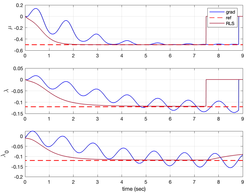
where $\theta^{*}=0.3$. $\theta_{0}=0.01$ is chosen as initial value for both schemes. $k_{1}=1.05,k_{2}=23,k_{3}=0.52$ are given. For RLS estimation based ES scheme, the following parameters are used: $k_{ls}=0.01$, $p_{0}=10^{3}$, and $\beta=0.98$ are given. For classical ES scheme, the following parameters are given: $k=0.08$, $\omega_{h}=0.6$, $\omega_{l}=0.8$, $S(t)=0.01\sin 3t$, and $M(t)=sin3t$. We apply the Gaussian measurement noise as ($\sigma=0.05$) for both gradient and RLS algorithms. We apply RLS estimation based ES scheme in Fig.3. The results for this example is given in Fig.6. It is obvious that proposed scheme can reach a neighborhood of the extremum point $\theta^{*}=0.3$ at $y^{*}=8.85$ less than 2 second while classical ES finds the extremum point very late and cannot maintain that extremum point under measurement noise.

Consider the following model

	$\displaystyle y$	$\displaystyle=y_{1}+y_{2},$		(35)
	$\displaystyle y_{1}$	$\displaystyle=am(u_{1}),\penalty\ m(u_{1})=(2m^{*}_{1}u^{*}_{1}u_{1})/(u^{*2}_{1}+u^{2}_{1}),$
	$\displaystyle y_{2}$	$\displaystyle=am(u_{2}),\penalty\ m(u_{2})=(2m^{*}_{2}u^{*}_{2}u_{2})/(u^{*2}_{2}+u^{2}_{2}),$
	$\displaystyle u$	$\displaystyle=[u_{1},\penalty\ u_{2}]=[\theta_{1},\penalty\ \theta_{2}].$

In this section, we also tested our ES scheme in ABS using MATLAB/Simulink. Then, we compared its performance with gradient based ES scheme developed by [1]. The wheel characteristics are given by the following set of equations

References

- [1] K. B. Ariyur and M. Krstic, Real-time Optimization by Extremum-Seeking Control. John Wiley & Sons, 2003.
- [2] H. Wang, M. Krstic, and G. Bastin, “Optimizing bioreactors by extremum seeking,” International Journal of Adaptive Control and Signal Processing, vol. 13, no. 651, p. 669, 1999.
- [3] G. Bastin, D. Nesic, Y. Tan, and I. Mareels, “On extremum seeking in bioprocesses with multivalued cost functions,” Biotechnology Progress, vol. 25, no. 3, pp. 683–689, 2009.
- [4] S. Drakunov, U. Ozguner, P. Dix, and B. Ashrafi, “Abs control using optimum search via sliding modes,” IEEE Transactions on Control Systems Technology, vol. 3, no. 1, pp. 79–85, 1995.
- [5] H. Yu and U. Ozguner, “Extremum-seeking control strategy for abs system with time delay,” in Proc. IEEE American Control Conference, vol. 5, 2002, pp. 3753–3758.
- [6] E. Dincmen, B. Guvenc, and T. Acarman, “Extremum-seeking control of abs braking in road vehicles with lateral force improvement,” IEEE Transactions on Control Systems Technology, vol. 22, no. 1, pp. 230–237, 2014.
- [7] E. Dincmen, “Adaptive extremum seeking scheme for abs control,” in 13th IEEE International Workshop on Variable Structure Systems, 2014, pp. 1–6.
- [8] C. Mayhew, R. Sanfelice, and A. Teel, “Robust source-seeking hybrid controllers for autonomous vehicles,” in Proc. IEEE American Control Conference, 2007, pp. 1185–1190.
- [9] C. Zhang and R. Ordonez, “Robust and adaptive design of numerical optimization-based extremum seeking control,” Automatica, vol. 45, no. 3, pp. 634–646, 2009.
- [10] J. Lin, S. Song, K. You, and M. Krstic, “Overshoot-free nonholonomic source seeking in 3-d,” International Journal of Adaptive Control and Signal Processing, vol. 31, no. 9, pp. 1285–1295, 2017.
- [11] E. Biyik and M. Arcak, “Gradient climbing in formation via extremum seeking and passivity-based coordination rules,” Asian Journal of Control, vol. 10, no. 2, pp. 201–211, 2008.
- [12] M. Stankovic and D. Stipanovic, “Stochastic extremum seeking with applications to mobile sensor networks,” in Proc. IEEE American Control Conference, 2009, pp. 5622–5627.
- [13] B. Moore and C. Canudas-de Wit, “Source seeking via collaborative measurements by a circular formation of agents,” in Proc. IEEE American Control Conference, 2010, pp. 6417–6422.
- [14] L. Fu and U. Ozguner, “Extremum seeking with sliding mode gradient estimation and asymptotic regulation for a class of nonlinear systems,” Automatica, vol. 47, no. 12, pp. 2595–2603, 2011.
- [15] B. G. B. Hunnekens, M. A. M. Haring, N. van de Wouw, and H. Nijmeijer, “A dither-free extremum-seeking control approach using 1st-order least-squares fits for gradient estimation,” in 53rd IEEE Conference on Decision and Control, 2014, pp. 2679–2684.
- [16] D. Nesic, T. Nguyen, Y. Tan, and C. Manzie, “A non-gradient approach to global extremum seeking: An adaptation of the shubert algorithm,” Automatica, vol. 49, no. 3, pp. 809–815, 2009.
- [17] M. Chioua, B. Srinivasan, M. Guay, and M. Perrier, “Performance improvement of extremum seeking control using recursive least square estimation with forgetting factor,” IFAC-PapersOnLine, vol. 49, no. 7, pp. 424–429, 2016.
- [18] D. Nesic, A. Mohammadi, and C. Manzie, “A framework for extremum seeking control of systems with parameter uncertainties,” IEEE Transactions on Automatic Control, vol. 58, no. 2, pp. 435–448, 2013.
- [19] P. Blackman, “Extremum-seeking regulators,” in An exposition of adaptive control. Macmillan, 1962.
- [20] M. Krstic, “Performance improvement and limitations in extremum seeking control,” Systems & Control Letters, vol. 39, no. 5, pp. 313–326, 2000.
- [21] M. Krstic and H. H. Wang, “Stability of extremum seeking feedback for general nonlinear dynamic systems,” Automatica, vol. 36, no. 4, pp. 595–601, 2000.
- [22] M. Guay, “A time-varying extremum-seeking control approach for discrete-time systems,” Journal of Process Control, vol. 24, no. 3, pp. 98–112, 2014.
- [23] M. Guay and D. Dochain, “A time-varying extremum-seeking control approach,” Automatica, vol. 51, pp. 356–363, 2015.
- [24] A. Ghaffari, M. Krstic, and D. Nesic, “Multivariable newton-based extremum seeking,” Automatica, vol. 48, no. 8, pp. 1759–1767, 2012.
- [25] P. Ioannou and B. Fidan, Adaptive Control Tutorial. Society for Industrial and Applied Mathematics, 2006.