How much is your Strangle worth?
On the relative value of the $\delta-$Symmetric Strangle under the Black-Scholes model

Options, as asset’s price derivatives, are the primary tools available to the market participants for hedging their portfolio from directional risk and/or volatility risk. The so-called option’s delta, which typically is denoted as $\delta$ or $\Delta$, measures the ’sensitivity’ of the option’s price to changes in the price of the underlying security, is the primary parameter one considers when using an option to mitigate directional risk. The option’s delta is seen as the hedging ratio and is often also used (near expiration) by market participants as a surrogate to the probability that the option will expire in the money. With standard option pricing model of Black and Scholes (1973), (abbreviated here as the BS model, see below), these probabilities are readily available for direct calculations under the governing log-normality assumption of the asset’s returns. Roughly speaking, a trader that sells (or buys) a put option at a strike located one standard deviation below the current asset’s price, ends up with a 16-delta put contract option (i.e. with $\delta=-0.16$). We denote the corresponding strike for this 16-delta put contract option as $k_{0.16}^{-}$. Similarly, a trader that sells (or buys) a call option at a strike located one standard deviation above the current asset’s price, ends up with a 16-delta call option (i.e. $\delta=0.16$). We denote the corresponding strike for this 16-delta call contract as $k_{0.16}^{+}$. Thus, the corresponding strangle, which is obtained by selling a (negative) 16-delta put option and a (positive) 16-delta call option, is a delta-neutral strategy that is associated, very roughly, with a 0.68 probability for the asset’s price to remain between the two strikes, $k_{0.16}^{-}$ and $k_{0.16}^{+}$ by expiration, all as resulting from the governing normal distribution assumption. We refer to such a strangle as a 16-delta Symmetric Strangle, only to indicate the common (absolute) delta value ($\delta=0.16$) of its put and call components.

In a similar fashion we use the term a $\delta-$Symmetric Strangle to indicate the strangle obtained, for some fixed $\delta\in(0,0.5)$, from buying (or selling) a $\delta$-units put and call option contracts at the corresponding strikes $k_{\delta}^{-}$ and $k_{\delta}^{+}$, respectively. Such a strangle would be a delta-neutral strategy offering zero directional risk but potentially useful for mitigating volatility risk. We further denote by $\Pi_{\delta}$ the price of (or the credit received from) such $\delta-$Symmetric Strangle. In this paper, we study, for a a given $\delta$, the value of this $\delta-$Symmetric Strangle relative to the width of the corresponding spread $(k_{\delta}^{+}-k_{\delta}^{-})$, adjusted for its present value (PV). More precisely, for any a $\delta\in(0,0.5)$, we define the relative value of the corresponding $\delta-$Symmetric Strangle as

In Section 2, we show that under the standard BS option pricing model, the strangle’s relative value, $R_{\delta}$, is independent of the price of the underlying security and is a function only of $\delta$ and the prevailing volatility used in the pricing model. In fact, as we will see in Theorem 1 below, for any given $\delta\in(0,0.5)$, we have $R_{\delta}\leq{\cal{R}}_{\delta}$ where

and where $\phi(\cdot)$ is the standard normal density ($pdf$), $\phi(u):=\frac{1}{\sqrt{2\pi}}e^{-\frac{u^{2}}{2}}$, and $z_{\delta}\equiv\Phi^{-1}(\delta)$, is usual $\delta^{th}$ percentile of the standard normal distribution, whose cumulative distribution function ($cdf$) is $\Phi(z):=\int_{-\infty}^{z}\phi(u)du$. We point out that since $\delta<0.5$, we have $z_{\delta}<0$ in expression (2) of ${\cal{R}}_{\delta}$.

As an illustration, one quickly finds by utilizing (2) that the $16$-delta Symmetric Strangle has a relative value of ${\cal{R}}_{0.16}=0.08467$ and that the $30$-delta Symmetric Strangle has a relative value of ${\cal{R}}_{0.30}=0.36$. That is to say that under the standard BS option pricing model, one would expect the price of the $30$-delta Symmetric Strangle to be at most 36% of the width of the spread between the corresponding strikes, irrespective of the security’s price, or time to expiry, and irrespective of the prevailing volatility. More generally, it follows from Theorem 1, that for a any given $\delta\in(0,\,0.5)$, the corresponding $\delta-$strangle’s price, $\Pi_{\delta}$, as calculated under the BS pricing model, satisfies

irrespective of the security’s price, or time to expiry, and irrespective of the prevailing volatility. In Section 3, we illustrate how this measure ${\cal{R}}_{\delta}$ in (2) may be used as a benchmark to assess the market pricing (or ’worthiness’) of the $\delta-$symmetric strangle compared to its (relative) price, $R_{\delta}$, as suggested by standard BS pricing model. The explicit expression of ${\cal{R}}_{\delta}$ as is given in (2) allow us to also address, in Section 4, the strangle’s exit strategy and the corresponding optimal choice of $\delta$ for it.

One of the most widely celebrated option pricing model for equities (and beyond) is that of Black and Scholes (1973). Their pricing model is derived under some simple assumptions concerning the distribution of the asset’s returns, coupled with presumptive continuous hedging, zero dividend, risk-free interest rate, $r$, and no cost of carry or transactions fees. While the aptness of these assumptions has often been criticized (see for example Yalincak (2012)), it has remained as a leading option pricing model for the retail trading practitioner (e.g.: Sinclair (2010)). However, in its standard form, the BS model evaluates, for a risky asset with a current market price $\mu$, the price of an European call option contract at a strike $k$ and $t$ days to expiration as:

Here, using the standard notation,

where $\sigma$ denotes the standard deviation of the daily asset’s returns, and $\Phi(\cdot)$ is the standard normal cdf defined above. The model for the corresponding price of a put option contract, $p_{\mu}(k)$, may be obtain from expression (3) of $c_{\mu}(k)$, by exploiting the so-called put-call parity which is expressed by the equation

see for example Jiang (2005, Theorem 2.3) or Peskir and Shiryaev (2002) for details. This parity implies that the price of the corresponding put option contract is,

There is substantial body of literature dealing with the BS option pricing model in (3)-(6), its refinements, its extensions and the so-called, its implied ’Greeks’ (i.e. the various partial derivatives of different orders, representing the model’s ”sensitivities” to changes in its parameters). The interested reader is referred to standard textbooks such as Wilmott, Howison, Dewynne (1995), Hull (2005), Jiang (2005) or Iacus (2011).

As we already mentioned in the Introduction, we focus our attention here on the option’s delta, which we denote by $\Delta$ as a function with a corresponding value of $\delta\in(0,1)$. More specifically, while suppressing (for sake of simplicity for now) from the notation $r,t$ and $\sigma^{2}$, we define for the call and the put contracts options their respective $\Delta$ functions as, $\Delta_{c}(k):={\partial c_{\mu}(k)}/{\partial\mu}$ and $\Delta_{p}(k):={\partial p_{\mu}(k)}/{\partial\mu}$. It follows immediately from the put-call parity equation in (5) that $\Delta_{p}(k)=-(1-\Delta_{c}(k))$. It is well known (see for Example, Jiang (2005)) that for the BS pricing model in (3), $\Delta_{c}(k)=\Phi(d_{1}(k))$, where $d_{1}(k)$ is given in (4), and hence $\Delta_{p}(k)=-(1-\Phi(d_{1}(k))\equiv-\Phi(-d_{1}(k))$.

For its supreme importance to portfolio hedging, the investor/trader often needs to buy (or sell) an option at a strike, $k$, which is associated with a specified and desired value $\delta$ of the option’s $\Delta$. For any given $\delta\in(0,1)$, we let $k^{+}_{\delta}$ denote the (unique) solution of the equation $\Delta_{c}(k^{+}_{\delta})=\delta$, or equivalently the solution of

Accordingly, it follows immediately that $k^{+}_{\delta}$ satisfies the equation

and hence, by utilizing (4) in (8) leads to the solution as

where we have substituted $\nu\equiv\sigma\sqrt{t}$ throughout. It should be clear from (9) that if $\delta<0.5$, one has $z_{\delta}<0$ and therefore $k^{+}_{\delta}>\mu$, so that the corresponding call option is said to be ’out of the money’ (OTM). Also, note that it follows from (4) and (8) that $d_{2}(k_{\delta}^{+})=d_{1}(k^{+}_{\delta})-\sigma\sqrt{t}\equiv z_{\delta}-\nu$, so that

in (3). Indeed, with the re-parameterization by $(\delta,\,\nu)$ (with $\nu\equiv\sigma\sqrt{t}$), of the BS option pricing model in (3), we may re-express, upon using the matching expressions (7)-(10) in equation (3), the current price of a $\delta-$unit call option in a much simpler form as

for any $\delta\in(0,1)$ and with $\nu>0$.

Similarly to (11), we calculate the current price of the $\delta-$unit put contract option by using the put-call parity equation in (5), and by noting that by (7) the corresponding $k^{-}_{\delta}$ strike for the put contract is the same as the strike $k^{+}_{1-\delta}$ of the $(1-\delta)-$unit call option contract, so that $k^{-}_{\delta}\equiv k^{+}_{1-\delta}$. Accordingly, since $z_{\delta}\equiv-z_{1-\delta}$, we obtain from (9) that

Hence, it follows immediately from (5) and (12), that under the $(\delta,\,\nu)$ re-parameterization, the expression for the current price of the $\delta-$unit put option is,

It should be clear from (12) that if $\delta<0.5$ and $r=0$, one has $z_{\delta}<0$ and therefore $k^{-}_{\delta}<\mu$ only if $\nu<-2\cdot z_{\delta}$, in which case, the corresponding put option is said to be ’out of the money’ (OTM). Hence, we will restrict our attention to the practical case of the above parametrization in which $(\delta,\nu)$ are such that $k^{-}_{\delta}<\mu<k^{+}_{\delta}$, or alternatively, $(\delta,\nu)\in{\cal B}$, where

We further point out that the two strikes, $k^{+}_{\delta}$ and $k^{-}_{\delta},(\equiv k^{+}_{1-\delta})$, need not be symmetrical with respect of the current price $\mu$ of the underlying security (i.e.: $\mu-k^{-}_{\delta}\neq k^{+}_{\delta}-\mu$). It is well-known that the occasional observed asymmetry of these equal $\delta-$ units strikes is a fixture of the skew in the volatility surface that is affecting the option pricing model, see for example Gatheral (2006), or Doran and Krieger (2010).

Consider now a trader that desires to simultaneously sells (say), at some given level of $\delta<0.5$, the $\delta-$unit put and the $\delta-$unit call contracts so as to form the ’OTM’ $\delta-$Symmetric Strangle strategy. The total selling price of this strangle as calculated under the BS pricing model, is therefore $\Pi_{\delta}=c_{\mu}(k^{+}_{\delta})+p_{\mu}(k^{-}_{\delta})$. As a measure for assessing the ’worthiness’ of this strangle, we consider the ’value’ of the selling price, $\Pi_{\delta}$, relative to the present value of the spread between the strikes, namely, $PV(k^{+}_{\delta}-k^{-}_{\delta})=(k^{+}_{\delta}-k^{-}_{\delta})\times e^{-rt}$. We express this relative value measure in (1) as

Note that by its definition, $R(\delta,\,\nu)\geq 0$ for all $\delta\in(0,0.5)$ and $\nu>0$, in particular over ${\cal B}$. Further, since an European option price is (linearly) homogeneous in $\mu$, and in the strike, $k$, (see Theorem 6 of Merton (1973)), the ratio $R(\delta,\nu)$ in (14), is independent of the current price, $\mu$, of the underlying security. Also note that since we account in (14) for the present value of the spread between the strikes, this quotient is, by construction, also independent of the risk-free interest rate, $r$. This can fully realized by substituting expressions (9), (11), (12) and (13) in $R(\delta,\,\nu)$ and simplifying the resulting terms, to obtain, for each $\delta<0.5$ and $\nu\equiv\sigma\sqrt{t}>0$, the expression,

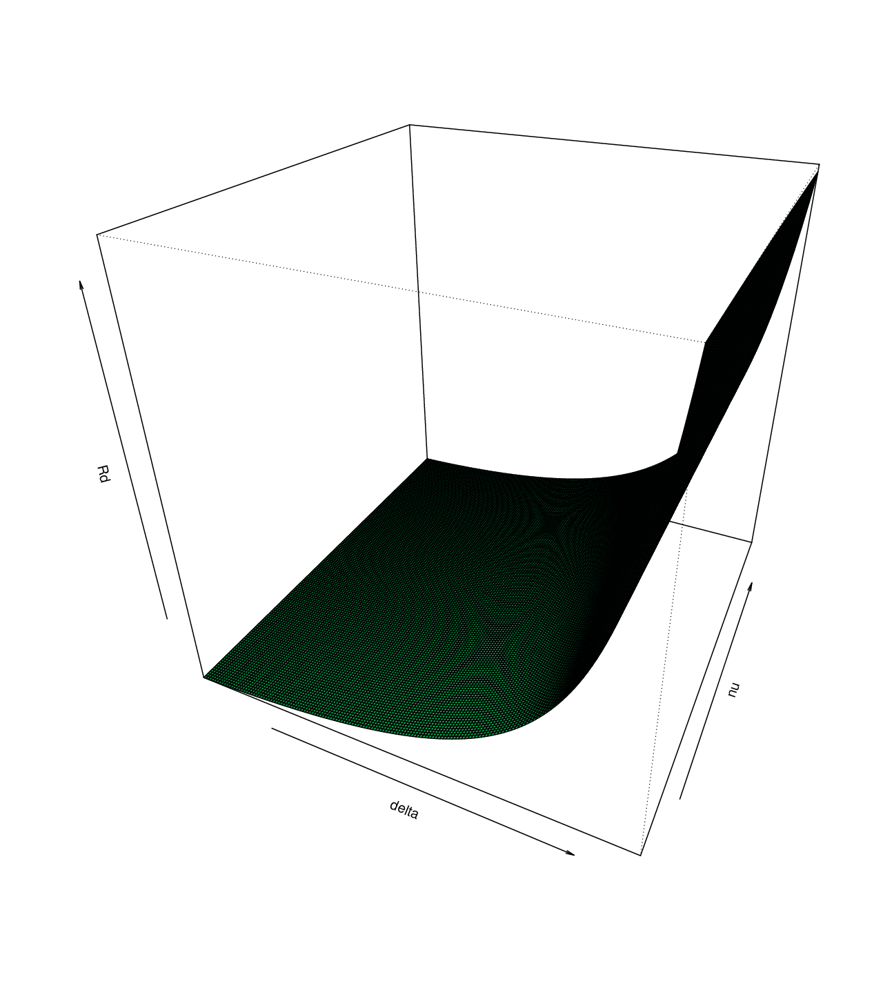
for the relative value of the $\delta-$Symmetric Strangle under the BS option pricing model. We point that the values of $R(\delta,\,\nu)$ in (15) are straightforward to calculate for any $(\delta,\nu)$. Figure 1 below provides the graph of $R(\delta,\,\nu)$ for various values of $(\delta,\nu)$, with $0<\delta<0.5$ and $0<\nu<1$, where $\nu=\sigma\sqrt{t}$ representing realistic values for $t$ (the time in days to expiry) and the model’s daily (implied or historical) volatility, $\sigma$. In any case, the properties of $R(\delta,\,\nu)$, as a function of $\delta$ and $\nu$ (in ${\cal B}$) are of interest. In Appendix A below we show that for a fixed $\delta<0.5$, $R(\delta,\nu)$ is monotonically non-increasing function of $\nu$ (with $\partial R/\partial\nu\leq 0$) and that for a fixed $\nu>0$, $R(\delta,\nu)$ is monotonically increasing function of $\delta$ (with $\partial R/\partial\delta>0$).

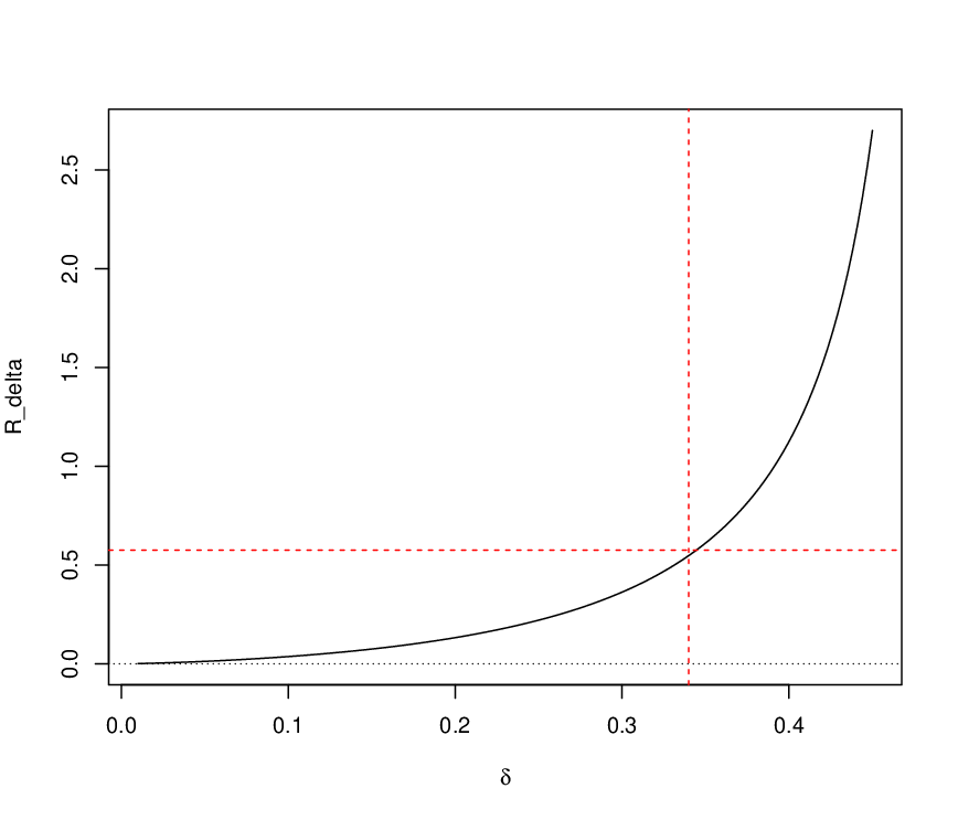
The results of Theorem 1 and the bound ${\cal{R}}_{\delta}$ in (16) provide a benchmark for assessing the value, in relative terms, of a $\delta-$Symmetric Strangle under the BS option pricing model in (3)-(6), as applicable to any security (i.e. independent of the current underlying security price $\mu$), to any expiry (independent of $t$), and under any presumed volatility (independent of $\sigma$). In fact, if $\hat{R}_{\delta}$ denotes the market (relative) value of a $\delta-$Symmetric Strangle (i.e. the market version of (1)), then, this strangle would be deemed ’well-priced’ compared to its (relative) price under the BS option pricing model, as long as $\hat{R}_{\delta}\geq{\cal{R}}_{\delta}$. In Figure 2 below, we graph the values of this function, ${\cal{R}}_{\delta}$ (in (16) or (2)) for all $0<\delta<0.5$.

The empirical (market) results exhibited in Table 1, illustrate the tremendous practical and strategy implications the results of Theorem 1 have. With such theoretical results at hand, retail traders and and market participants are now able to quickly assess whether or not the strangle they buy (or sell) is overpriced or under-priced in the market as compared to its Black-Scholes price, regardless the market volatility, the duration of the contract or the underlying assest’s price . It provides for a common benchmark for assessing and comparing the market (relative) pricing of a major trading strategy (namely the $\delta-$Symmetric Strangle) across various securities and assets, across various durations and irrespective of the underlying security-specific volatility (implied or historical).

One of the appealing aspects of a $\delta-$Symmetric Strangle is that from the outset, it is a delta-neutral strategy with zero directional risk, initially. Moreover a trader that sells such a strangle, for some fixed $\delta<0.5$, at the matching two strikes $k^{-}_{\delta}$ and $k^{+}_{\delta}$, benefit from a well defined probability of success, that may be calculated under the current distribution of the asset’s returns implied by BS option pricing model in (3) and (6). Specifically, for a given value $\delta<0.5$ and $\nu>0$, the initial probability that the underlying security price would remain, at expiration, between $k^{-}_{\delta},\ (\equiv k^{+}_{1-\delta})$ and $k^{+}_{\delta}$ is simply (see Remark 1),

Hence, the expected reward for a trader that sells the strangle for $\Pi_{\delta}=c_{\mu}(k^{+}_{\delta})+p_{\mu}(k^{-}_{\delta})$ (as credit) and plans to exit and buy it back for a fraction $\lambda\in(0,1]$ of the credit received is

In relative terms, this expected reward, relative to the present value of the spread between the strikes, becomes

where ${\cal{R}}_{\delta}$ is given in (2). As was mentioned in the Introduction and pointed out in Remark 1, for small values of $\nu$ (i.e. near expiration) we may approximate the ’success’ probability in (18) as $\alpha\approx(1-2\delta)$. Accordingly, for any given fractional loss $\lambda\in(0,1]$ the expected relative reward in (19), under this approximation would be,

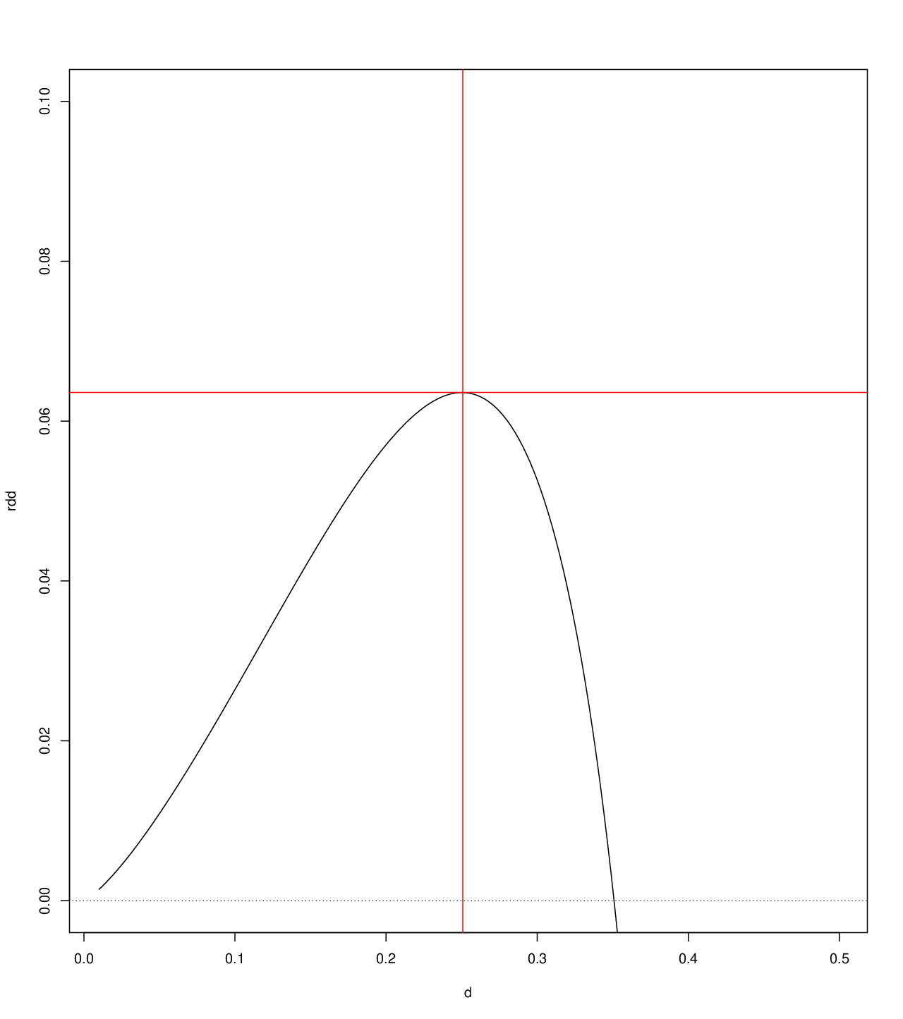
Observe that ${\cal E}_{\lambda}(\delta)\geq 0$ as long as $\delta\leq 1/2(1+\lambda)$ and that, upon using (16) and (17), the equation

is seen to have a unique root, $\delta^{*}$, at which point ${\cal E}_{\lambda}(\delta)$ attains its maximal value. That is, for a given fractional lose $\lambda\in(0,1]$, this root $\delta^{*}=h(\lambda)$, must solves the equation

at which point ${\cal E}^{*}_{\lambda}:={\cal E}_{\lambda}(\delta^{*})\geq{\cal E}_{\lambda}(\delta)$.

In Figure 3 above we present the graph of the relative reward function, ${\cal E}_{\lambda}(\delta)$, for a trader who sells a $\delta-$Symmetric Strangle, and wishes, as a matter of strategy, to exit it upon a loss of 50% of the credit received. This case corresponds to $\lambda=0.5$ and results with an optimal choice for $\delta$ of $\delta^{*}=0.2336$ for this strategy to yield a maximal expected relative reward of ${\cal E}^{*}_{0.5}=0.05615$.

In Table 2 below, we provide the ’optimal’ values for $\delta$ as were calculated (as a numerical solution of (21)) for various choices of $\lambda$, along with the corresponding values of the maximal expected reward ${\cal E}^{*}_{\lambda}$, and the matching initial probability of ”success” of this $\delta^{*}-$ Symmetric Strangle strategy. As can be seen from Table 1, the selling of a ’standard’ 16-delta symmetric strangle with its $0.68$ ’success’ probability should be coupled with an exit strategy that limits losses at 100% of the credit received may yield a maximal expected relative reward of ${\cal E}^{*}_{1}=0.031$. In contrast, the selling of a 30-delta symmetric strangle of the lesser ’success’ probability (of 0.4) should be coupled with an exit strategy that limits losses at 25% of the credit received, but may triple the maximal expected reward to ${\cal E}^{*}_{0.25}=0.091$

In this appendix we study the coordinate-wise behavior of $R(\delta,\nu)$ as given in (15) over the practical domain ${\cal B}$. To begin with, note first that since

we may express $R(\delta,\,\nu)$ in (15), entirely in terms of the standard normal $pdf$ and $cdf$, as

Upon differentiating expression (22) of $R(\delta,\nu)$, with respect to $\delta$ and with respect to $\nu$ along with the fact that $\phi^{\prime}(u):=\frac{d}{du}\phi(u)=-u\phi(u)$ we obtain the following results.

References

- [1] Black F., and Scholes M., (1973). The pricing of options and corporate liabilities. The Journal of Political Economy, 637-654.
- [2] Doran, J., and Krieger, K., (2010). Implications for Asset Returns in the Implied Volatility Skew. Financial Analysts Journal, 66(1), 65-76.
- [3] Gatheral, J., (2006). The Volatility Surface, John Wiley and Sons, NJ.
- [4] Hull, C. J., (2017). Options, Futures and Other Derivatives, 10th Ed, Pearson, NY.
- [5] Iacus, M. S., (2011). Option Pricing and Estimation of Financial Models with R, John Wiley and Sons, NY.
- [6] Jiang, L. (2005). Mathematical Modeling and Methods of Option Pricing, Translated from Chinese by Li. C, World Scientific, Singapore.
- [7] Merton, R., (1973). Theory of rational option pricing. The Bell Journal of Economics and Management Science, 141-183.
- [8] Peskir, G. and Shiryaev, A., (2002) A Note on the Call-Put Parity and a Call-Put Duality. Theory of Probability and Its Applications , Vol 46(1), 167-170.
- [9] Sinclair, E., (2010). Option Trading; Pricing and Volatility Strategies and Techniques John Wiley and Sons, NJ
- [10] Wilmott, P., Howison, S. and Dewynne, J., (1995). The Mathematics of Financial Derivatives: A Student Introduction, 1st Ed, Cambridge University Press.
- [11] Yalincak, H. O., (2012). Criticism of the Black-Scholes Model: But Why is It Still Used?: (The Answer is Simpler than the Formula). Available at SSRN: https://papers.ssrn.com/sol3/papers.cfm?abstract_id=2115141