Limiting distributions for eigenvalues of sample correlation matrices from heavy-tailed populations

As seen in the above discussion, the sample correlation matrix ${\mathbf{R}}$ has mainly been studied under the finite fourth moment assumption. In the intermediate regime, where $\mathbb{E}\xi^{4}=\infty$ and $\mathbb{E}\xi^{2}<\infty$, the limiting spectral distribution is known to be the MP law and [18] studied the extreme eigenvalues. Under infinite variance, the limiting spectral distribution of ${\mathbf{S}}$ has been characterized, whereas no results on the sample correlation matrix ${\mathbf{R}}$ seem to be available in the literature.

By assuming that the distribution of $\xi$ is symmetric and regularly varying with index $\alpha\in(0,2)$, we establish in this paper that the sequence of ESDs $F_{{\mathbf{R}}}$ converges weakly to a new distribution $H_{\alpha,\gamma}$ termed as $\alpha$-heavy MP law with parameter $\gamma$. This result is introduced in Section 2.1 (Theorem 2.1) where comparison with the MP law $\sigma_{MP,\gamma}$ is also proposed. Theorem 2.2 shows that the class of distributions $H_{\alpha,\gamma}$ can be extended continuously at the boundaries $\alpha=2$ and $\alpha=0$, yielding the MP law $\sigma_{MP,\gamma}$ and a modified Poisson distribution, respectively. Subsequently in Section 2.2, we propose a consistent estimator for the tail index $\alpha$.

The remaining sections of the paper are devoted to the proofs of Theorems 2.1 and 2.2. Our main tool is a moment method that required a specific and careful counting of relevant graphs to cope with exploding second moments of the matrix entries $\{X_{ij}\}$. Section 3 presents the main steps of this moment method based on a path-shortening algorithm that was developed in [18]. Section 4 establishes the combinatorics on associated graph counting for the moment method by using set partitions. The proof of our main result Theorem 2.1 is then completed in Section 5, which also contains the formula for the moments of the $\alpha$-heavy MP laws $H_{\alpha,\gamma}$. Finally, Section 6 proves Theorem 2.2.

Recall that for $\gamma>0$ the Marčenko–Pastur law $\sigma_{MP,\gamma}$ is

where the density of the absolutely continuous part is

with $a_{\gamma}=(1-\sqrt{\gamma})^{2}$ and $b_{\gamma}=(1+\sqrt{\gamma})^{2}$. Its moments are

.

In this paper we find a family of new distributions $\{H_{\alpha,\gamma}\}$ for parameters $\alpha\in(0,2)$ and $\gamma>0$. We call $H_{\alpha,\gamma}$ the $\alpha$-heavy MP law with parameter $\gamma$. Each $H_{\alpha,\gamma}$ is entirely determined by its moment sequence $\mu_{k}(\alpha,\gamma)=\int x^{k}\,\mathrm{d}H_{\alpha,\gamma}(x)$, $k\geq 1$. The exact expression for $\mu_{k}(\alpha,\gamma)$ requires a considerable amount of additional notation: it is given in (5.1). Roughly speaking, $\mu_{k}(\alpha,\gamma)$ can be decomposed into a Marčenko–Pastur part and a heavy tail part as follows

where $d_{k}(\alpha,\gamma)>0$ is given in (5.1). Formula (5.1) is explicit and requires some counting that can be implemented using computing software. For small values of $k$, $d_{k}(\alpha,\gamma)$ can be evaluated directly. In Section 5.1, we derive that

The following theorem is the main result of the paper.

The symmetry requirement on the distribution of $\xi$ is technical. It allows to neglect all expectations of odd powers of matrix entries in our moment method. Since the moment formula (3.2) which is a key ingredient of the proof only depends on the distribution of $\xi^{2}$ (and not $\xi$), the symmetry restriction can likely be removed and Theorem 2.1 also holds for non-symmetrically distributed $\xi$; see Remark 3.6 for details.

We now give some illustrations of the theorem and compare the limiting $\alpha$-heavy MP laws $H_{\alpha,\gamma}$ with the classical MP laws.

Figure 1 shows the shape of $H_{\alpha,\gamma}$ for different values of $\alpha$, $p=1000,n=5000$ and $\gamma=p/n$. The entries $X_{ij}$ were drawn from a $t$-distribution with $\alpha\in\{1.5,1,0.5,0.1\}$ degrees of freedom. We compare the (normalized) histogram of the eigenvalues $(\lambda_{i}({\mathbf{R}}))$ with the Marčenko–Pastur density $f_{p/n}(x)$. The parameter $\gamma=p/n=0.2$ is the same in the four plots in Figure 1 as well as the four MP densities despite their visual difference due to different scales used in the plots. Observe that for $\alpha=1.5$ (top left panel) the histogram resembles $f_{p/n}$ at first sight. At closer inspection one notices that the $\alpha$-heavy MP law has a larger support than the MP law. Moreover, more mass is concentrated around the mean 1. These two effects become more pronounced if the tail heaviness of $\xi$ increases, i.e. $\alpha$ decreases. The plots show that most mass is concentrated around 1 if $\alpha$ is small.

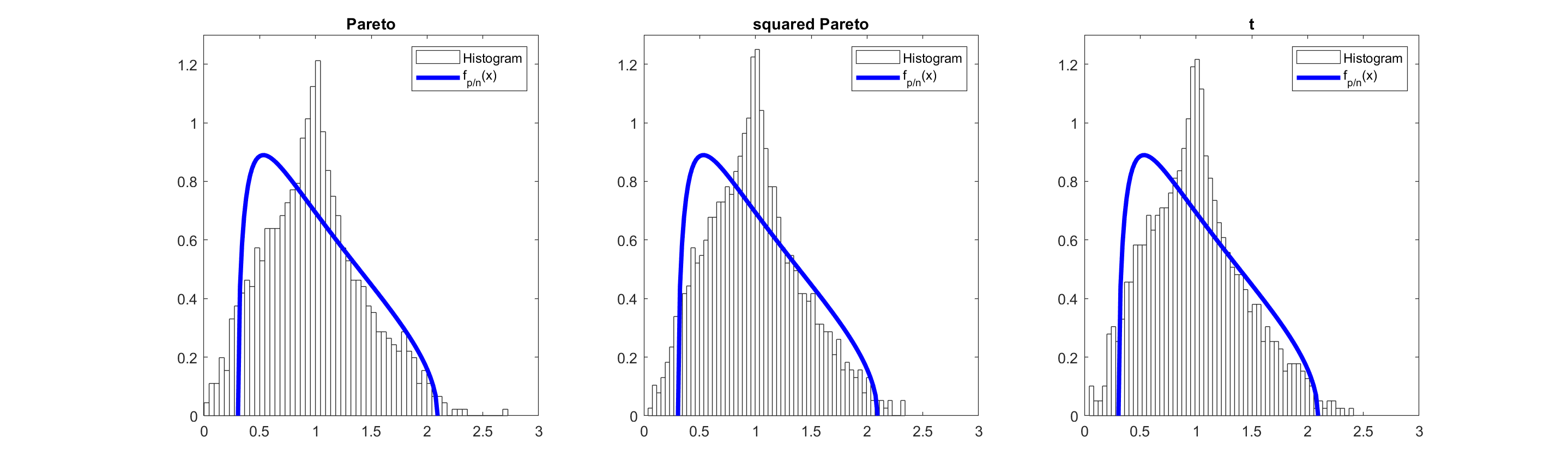
In Figure 2 we consider the spectral distribution of ${\mathbf{R}}$ for non-symmetric distributions of $\xi$. The left and middle plots in Figure 2 are generated with non-symmetrically distributed $\xi$’s that are regularly varying with index $\alpha=1.1$. For the right plot, the symmetric $t$-distribution with $\alpha$ degrees of freedom was used for which Theorem 2.1 shows the convergence of the ESD to the $\alpha$-heavy MP law. We observe that that the three ESDs look almost identical, which suggests that the symmetry assumption in Theorem 2.1 can indeed be relaxed.

Theorem 2.1 also yields the limits of the empirical moments $m_{k}({\mathbf{R}}):=p^{-1}\sum_{i=1}^{p}(\lambda_{i}({\mathbf{R}}))^{k}$ for $k\geq 1$. More precisely, in the course of its proof we will show that $m_{k}({\mathbf{R}})$ converges in probability to $\mu_{k}(\alpha,\gamma)$. Note that the case $k=1$ is trivial since $m_{k}({\mathbf{R}})=1$. In Figure 3, we place ourselves in the setting of the top right panel of Figure 1 ($\alpha=1$). That is, we pick $p=1000,n=5000$ and simulate the iid entries of ${\mathbf{X}}^{(j)}$ from a $t(1)$ distribution. Then we compute the eigenvalues $\lambda_{1}({\mathbf{R}}^{(j)}),\ldots,\lambda_{p}({\mathbf{R}}^{(j)})$. This procedure is repeated until we have $L=1000$ samples

from which we calculate $m_{k}({\mathbf{R}}^{(j)})$, $1\leq j\leq L$ for $k\in\{2,3,4,5\}$. The first row in Figure 3 shows the (normalized) histograms of $m_{k}({\mathbf{R}}^{(j)})$, ($1\leq j\leq L$). By Theorem 2.1, the limits (in probability) of $m_{k}({\mathbf{R}}^{(j)})$ are

where $\mu_{k}$ is a shorthand notation for $\mu_{k}(1,0.2)$. Vertical lines at values $\mu_{k}$ were added to the histograms in the first row. The averaged empirical moments

are very close to their limits $(\mu_{2},\mu_{3},\mu_{4},\mu_{5})$.

To obtain the second row in Figure 3, we simulated from a standard normal distribution instead of the $t(1)$ distribution. In this case the theoretical limiting moments are the Marčenko–Pastur moments $\beta_{k}:=\beta_{k}(0.2)$,

and the averaged empirical moments are $(1.1998,1.6393,2.4462,3.8776)$. It is interesting to note the different scaling on the $x$-axis when comparing the first and the second row of plots in Figure 3. In case of normal data, the spread is much smaller than for the heavy-tailed $t$-distribution. For $k\in\{4,5\}$ the $m_{k}$ fluctuate around different means since $d_{k}(1,0.2)>0$; see (2.1).

Our next result shows that the family of $\alpha$-heavy MP laws $\{H_{\alpha,\gamma}\}$ can be continuously extended at its boundaries $\alpha\in\{0,2\}$.

The proof of Theorem 2.2 is given in Section 6. Theorem 2.2 shows that $H_{\alpha,\gamma}$ interpolates between the (modified) Poisson and the Marčenko–Pastur distribution which are the boundary cases for $\alpha\to 0^{+}$ and $\alpha\to 2^{-}$.

Note that $1-\frac{1}{\gamma}+\frac{1}{\gamma}e^{-\gamma}>0$ for $\gamma>0$. Compared with the Poisson distribution with parameter $\gamma$, the modified Poisson distribution $q_{\gamma}$ has the masses at $k\geq 1$ scaled by the factor $1/\gamma$, a magnification when $\gamma<1$ and a shrinkage otherwise. It has mean $1$ which is very natural. Indeed, the $H_{\alpha,\gamma}$ distributions all have mean $1$. In particular when $\gamma\to 0$, $q_{\gamma}$ degenerates to the Dirac mass at 1.

Figure 4 shows normalized histograms of the spectrum of ${\mathbf{R}}$ for various values of $p,n$ and $\alpha=0.05$. The plots nicely illustrate the convergence to the modified Poisson distribution. In the top left panel, the bars at 0 and 1 are of about the same height. This is in perfect agreement with the point masses of the Poisson$(1)$ distribution at 0 and 1 which both are $\e^{-1}$. We also see that the smaller the ratio $p/n$, higher the concentration of the eigenvalues around the mean 1.

In this section, we develop a simple application of our general result to the problem of estimation of the tail index parameter $\alpha$. As discussed earlier, the empirical moments $m_{k}({\mathbf{R}}):=p^{-1}\sum_{i=1}^{p}(\lambda_{i}({\mathbf{R}}))^{k}$ for $k\geq 1$ converge in probability to the corresponding moments $\mu_{k}(\alpha,\gamma)$ of the limiting $\alpha$-heavy MP law. Note that for $k\geq 4$, $\mu_{k}(\alpha,\gamma)$ is a bijective function of $\alpha$ for any fixed ratio parameter $\gamma$. Let $\gamma_{n}=p/n$ be the actual dimension ratio. Define $\hat{\alpha}_{n}$, the method of moment estimator of $\alpha$, as the solution of

The previous discussion readily yields the consistency of this moment estimator.

For illustration purpose, we consider hereafter the case of $k=5$ with $\mu_{5}(\alpha,\gamma)$ as in (2.1) and (2.6). Then the estimator is explicitly given by

where $\beta_{5}(\gamma)$ is the fifth moment of the MP law (see (2.2)).

A small simulation experiment is conducted to check the finite-sample performance of the estimator. The experimental design is as follows.

• •

  Independent entries are simulated with Student $t(\alpha)$ distributions with $\alpha\in\{0.5,1,1.5\}$;

• •

  The dimension ratio is fixed to $n=2p$ with $p$ varying from 100 to 800 (thus $n$ runs from 200 to 1600);

• •

  For each combination, the estimator $\hat{\alpha}_{n}$ is averaged over 1000 independent replications.

These estimates are reported in Table 1 and plotted in Figure 5. One can observe the consistency of the estimator. However, it is also noticed that this convergence is in general slow which is indeed expected for heavy tailed entries.

In order to compute the limit of $\mathbb{E}[m_{k}]$, we perform a series of simplifying steps that innovatively use the inherent structure of self-normalized random variables and combine them with a moment formula derived from [1] for the product of the $Y$’s on the right-hand side of (3.1). In Section 3.1, we define the function

for a so-called path $I=(i_{1},\ldots,i_{k})$ and study properties of $F(I)$. We employ two reduction steps which mainly use the fact that $Y_{11}^{2}+\cdots+Y_{1n}^{2}=1$ to simplify $F(I)$. More precisely, we transform the path $I$ to a shorter path $\widetilde{I}$ in such a way that $F(I)$ can be obtained from $F(\widetilde{I})$. Depending on their reducibility, we distinguish between three classes of paths: completely reducible paths, irreducible paths and partially reducible paths. It is noteworthy that the completely reducible paths eventually yield the $k$-th Marčenko–Pastur moment $\beta_{k}(\gamma)$. Our path-shortening procedure is applicable to sample correlation matrices as long as the distribution of $\xi$ is symmetric. Under finite variance, one may deduce from Remark 3.2 that $\mathbb{E}[m_{k}]$ tends to $\beta_{k}(\gamma)$ since only the completely reducible paths contribute to the limit. The main challenge in the infinite variance case, where $\xi$ is regularly varying with index $\alpha\in(0,2)$, lies in the fact that all paths $I$ have a non-negligible contribution (see (3.9)). By (3.2) and the path-shortening procedure, the contribution of $F(I)$ to the sum in (3.1) depends only on the shortened path $\widetilde{I}$ and $\alpha$. Therefore, we need some rather involved combinatorics to accurately count how many $I$’s reduce to the same $\widetilde{I}$ under the path-shortening procedure. To this end, the first part of Section 4 establishes the combinatorics on associated graph counting by using set partitions. The remainder of Section 4 is devoted to the calculation of $F(I)$, ultimately culminating in Proposition 4.13 which is the crucial auxiliary result in the proof of Theorem 2.1. All our path-shortening steps in Section 3 and combinatorics in Section 4 are illustrated by additional examples for the reader’s convenience. The proof of Theorem 2.1 is then completed in Section 5.

To compute the expectation of $m_{k}$, we need to understand the even moments of products of self-normalized $Y_{ij}$’s. Assuming that $\xi$ is regularly varying with index $\alpha<2$, Albrecher and Teugels [1, p. 4] derived the following formula for the moments of the self-normalized random variables

where $k\geq 1$, $1\leq r\leq k$, $k_{i}\geq 1$ and $k_{1}+\cdots+k_{r}=k$; and $\Gamma(\cdot)$ denoting the gamma function. In particular, we have

It is interesting to compare the values in (1.4) and (3.2) with their counterparts from a Gaussian random variable $\xi\sim N(0,1)$. In this case the vector $(Y_{11},\ldots,Y_{1n})$ has the Haar distribution on the unit sphere ${\mathcal{S}}_{n-1}$. It is well-known that $\mathbb{E}[Y_{11}^{4}]=3/(n(n+2))$; thus $\lim_{n\to\infty}n\,\mathbb{E}[Y_{11}^{4}]=0$. Moreover, by [18, Example 2.1] we have

Note that $\mathbb{E}[Y_{11}^{2k_{1}}Y_{12}^{2k_{2}}\cdots Y_{1r}^{2k_{r}}]$ is of order $n^{-(k_{1}+\cdots+k_{r})}$. Unless all $k_{i}$’s are $1$, this is much smaller than what we obtained in (3.2) for $\xi$ regularly varying with index $\alpha<2$, where the same expectation was of order $n^{-r}$.

In this subsection, we will revisit the path-shortening algorithm developed in [18]. Some terminology from graph theory and notation is useful. The set of the first $m$ positive integers is denoted by ${[\![1,m]\!]}$. A tuple $I=(i_{1},i_{2},\ldots,i_{k})\in{{[\![1,p]\!]}}^{k}$ of positive integers is a path with vertices $i_{\ell}\in{[\![1,p]\!]}$. Its length is $k=|I|$. The set of distinct elements in $I$ is denoted by $\{I\}$. For any set $A$, we denote its cardinality by $\#A$. If $r=\#\{I\}$, $I$ is called an $r$-path. For example, $I=(1,1,2,2)$ has length 4; it is a 2-path since $\{I\}=\{1,2\}$. A path is canonical if $i_{1}=1$ and $i_{l}\leq\max\{i_{1},\ldots,i_{l-1}\}+1$, $l\geq 2$. A canonical $r$-path $I$ satisfies $\{I\}={[\![1,r]\!]}$.

Two paths are isomorphic if one becomes the other by a suitable permutation on ${[\![1,p]\!]}$. For example, $(9,6,9,6)$ and $(1,2,1,2)$ are isomorphic, but only the latter is canonical. Each isomorphism class contains exactly one canonical path. Given a canonical path with vertices ${[\![1,r]\!]}$ (a $r$-path), its isomorphic class of paths in ${{[\![1,p]\!]}}^{k}$ has exactly $p(p-1)\cdots(p-r+1)$ distinct elements: this corresponds to the number of injective maps from ${[\![1,p]\!]}$ to ${[\![1,r]\!]}$. Let $\mathcal{J}_{r,k}(p)$ denote the set of all $r$-paths $I\in{[\![1,p]\!]}^{k}$. We then have the disjoint union

For the reason just explained, it holds that

where

For more details and examples of these path notions consult Section 2.1.2 in [4].

Each summand in (3.1) corresponds to a path $I=(i_{1},i_{2},\ldots,i_{k})$ with vertices in ${[\![1,p]\!]}$ and a path $T=(t_{1},i_{2},\ldots,t_{k})$ with vertices in ${[\![1,n]\!]}$. Let

where the dependence on $n$ is suppressed in our notation. Note that on the right-hand side of (3.7) we have $|I|=k$; but we prefer to write $|I|$ to indicate that $F$ can be applied to paths of any length. By convention, $\emptyset$ denotes the empty path and we set $F(\emptyset)=n$.

By (3.1), we have then

We rewrite $\mathbb{E}[m_{k}]$ by sorting according to the number of distinct components in the path $I$. Note that $F(I_{1})=F(I_{2})$ if $I_{1}$ and $I_{2}$ are isomorphic. In view of (3.4), we see that

Therefore, the main task is to determine the function $F(I)$ for $I\in\mathcal{C}_{r,k}$. Assume that the symmetrically distributed $\xi$ is regularly varying with index $\alpha<2$. Using the moment formula (3.2) it is easy to see that every $I\in\mathcal{C}_{r,k}$ has a non-negligible contribution to the limit of $\mathbb{E}[m_{k}]$. Indeed, since $p$ and $n$ are proportional, we have for $I\in\mathcal{C}_{r,k}$,

where $N_{i}\geq 1$ counts the number of occurrences of the integer $i$ in $I$; compare also (3.13) later on. Different paths $I_{1},I_{2}\in\mathcal{C}_{r,k}$ will in general lead to different limits of $p^{r-1}F(I_{1})$ and $p^{r-1}F(I_{2})$.

In what follows, we will present several simplifications that can be applied in the calculation of $F(I)$.

• •

  In Section 3.2, we introduce a function $S$ which transforms a path $I$ into a certain path $S(I)$ of shorter length. A simple relation between $F(I)$ and $F(S(I))$ is derived.

• •

  In Section 3.3, this relation is applied to simplify the computation of $\mathbb{E}[m_{k}]$.

In this paper we will heavily consider a class of so-called $\Delta$-graphs defined as follows [4, Section 2.1.2]. Let $(I,T)$ be a pair of paths of length $k$ with vertices in ${[\![1,p]\!]}$ and ${[\![1,n]\!]}$, respectively. Plot the $i_{\ell}$ vertices and $t_{\ell}$ vertices on two parallel lines. For each $1\leq\ell\leq k$, draw a down-edge from $i_{\ell}$ to $t_{\ell}$, and an up-edge from $t_{\ell}$ to $i_{\ell+1}$. This is the $\Delta$-graph associated to the pair $(I,T)$, denoted as $\Delta(I,T)$. An example of such a graph with $k=3$ is given in Figure 6.

Furthermore, we remove the orientation of edges: an edge $e=(i,t)\in\Delta(I,T)$ means either a down-edge $i{\searrow}t$ or an up-edge $t{\nearrow}i$. Recall that the rows of ${\mathbf{Y}}=(Y_{it})$ are independent. Using $\Delta$-graphs, the product in (3.6) can be expressed as

where $m_{it}(I,T)$ is the degree of the edge $(i,t)$ in the graph $\Delta(I,T)$.

For future considerations we define the so-called skeleton $\Delta^{0}(I,T)$ of the graph $\Delta(I,T)$, which is constructed from $\Delta(I,T)$ by setting all degrees $m_{it}$ equal to $1$. In other words, all multiple edges in $\Delta(I,T)$ are glued together. By construction, $\Delta^{0}(I,T)$ is a connected graph with the same vertices as $\Delta(I,T)$. Finally, we write $N_{e}(I,T)$ for the number of edges of $\Delta^{0}(I,T)$.

The matrix ${\mathbf{Y}}=(Y_{it})$ possesses the following properties:

1. (1)

   By symmetry of the entry distribution we have for $s\leq n$ that $\mathbb{E}[Y_{i1}^{m_{1}}\cdots Y_{is}^{m_{s}}]=0$ if at least one exponent $m_{j}\in\mathbb{N}$ is odd.

2. (2)

   ${\mathbf{Y}}$ has independent rows.

3. (3)

   By definition, $\sum_{t=1}^{n}Y^{2}_{it}=1$ for each row $i$.

Assume that in a $\Delta(I,T)$ graph, there is an edge $(i,t)$ with odd degree, say $2s_{it}+1$. By (3.13) and property (1), $f(I,T)=0$ and this graph will not contribute to $F(I)$. Therefore, in the remaining discussions, we may assume that all degrees $m_{it}=2s_{it}$ are even. It follows by (3.2) that

for some positive constant $\theta(I,T)$. Therefore, $f(I,T)>0$ will be of highest order if $N_{e}(I,T)$ is minimal.

References

- [1] [author] Albrecher, HansjörgH. and Teugels, Jozef LJ. L. (2007). Asymptotic analysis of a measure of variation. Theory of Probability and Mathematical Statistics 74 1–10.
- [2] [author] Anderson, T. W.T. W. (2003). An Introduction to Multivariate Statistical Analysis, 3rd ed. John Wiley & Sons, Hoboken, New Jersey.
- [3] [author] Auffinger, AntonioA., Ben Arous, GérardG. and Péché, SandrineS. (2009). Poisson convergence for the largest eigenvalues of heavy tailed random matrices. Ann. Inst. Henri Poincaré Probab. Stat. 45 589–610. 10.1214/08-AIHP188 2548495 (2011b:60021)
- [4] [author] Bai, ZhidongZ. and Silverstein, Jack W.J. W. (2010). Spectral Analysis of Large Dimensional Random Matrices, second ed. Springer Series in Statistics. Springer, New York. 10.1007/978-1-4419-0661-8 2567175 (2011d:60014)
- [5] [author] Bai, Z. D.Z. D. and Silverstein, J. W.J. W. (2004). CLT for linear spectral statistics of large-dimensional sample covariance matrices. Ann. Probab. 32 553-605.
- [6] [author] Bai, Z. D.Z. D. and Yin, Y. Q.Y. Q. (1988). Necessary and sufficient conditions for almost sure convergence of the largest eigenvalue of a Wigner matrix. Ann. Probab. 16 1729–1741.
- [7] [author] Bai, Z. D.Z. D. and Yin, Y. Q.Y. Q. (1993). Limit of the smallest eigenvalue of a large-dimensional sample covariance matrix. Ann. Probab. 21 1275–1294. 1235416
- [8] [author] Bao, Z.Z., Pan, G.G. and Zhou, W.W. (2012). Tracy-Widom law for the extreme eigenvalues of sample correlation matrices. Electronic Journal of Probability 17.
- [9] [author] Basrak, BojanB., Cho, YeonokY., Heiny, JohannesJ. and Jung, PaulP. (2021). Extreme eigenvalue statistics of m-dependent heavy-tailed matrices. 57 2100–2127.
- [10] [author] Belinschi, SerbanS., Dembo, AmirA. and Guionnet, AliceA. (2009). Spectral measure of heavy tailed band and covariance random matrices. Comm. Math. Phys. 289 1023–1055. 10.1007/s00220-009-0822-4 2511659 (2010e:60011)
- [11] [author] Ben Arous, GérardG. and Guionnet, AliceA. (2008). The spectrum of heavy tailed random matrices. Comm. Math. Phys. 278 715–751. 10.1007/s00220-007-0389-x 2373441 (2008j:60015)
- [12] [author] Comtet, LouisL. (1974). Advanced Combinatorics. D. Reidel Publishing Company.
- [13] [author] Davis, Richard A.R. A., Heiny, JohannesJ., Mikosch, ThomasT. and Xie, XiaoleiX. (2016). Extreme value analysis for the sample autocovariance matrices of heavy-tailed multivariate time series. Extremes 19 517–547. 10.1007/s10687-016-0251-7 3535965
- [14] [author] El Karoui, NoureddineN. (2009). Concentration of measure and spectra of random matrices: applications to correlation matrices, elliptical distributions and beyond. Ann. Appl. Probab. 19 2362–2405. 10.1214/08-AAP548 2588248
- [15] [author] Gao, J.J., Han, X.X., Pan, G.G. and Yang, Y.Y. (2017). High dimensional correlation matrices: the central limit theorem and its applications. Journal of the Royal Statistical Society. Series B: Statistical Methodology 79 677-693.
- [16] [author] Giné, EvaristE., Götze, FriedrichF. and Mason, David M.D. M. (1997). When is the Student -statistic asymptotically standard normal? Ann. Probab. 25 1514–1531. 10.1214/aop/1024404523 1457629
- [17] [author] Heiny, JohannesJ. and Mikosch, ThomasT. (2017). Eigenvalues and eigenvectors of heavy-tailed sample covariance matrices with general growth rates: The iid case. Stochastic Process. Appl. 127 2179–2207. 10.1016/j.spa.2016.10.006 3652410
- [18] [author] Heiny, JohannesJ. and Mikosch, ThomasT. (2018). Almost sure convergence of the largest and smallest eigenvalues of high-dimensional sample correlation matrices. Stochastic Process. Appl. 128 2779–2815. 10.1016/j.spa.2017.10.002 3811704
- [19] [author] Heiny, JohannesJ. and Mikosch, ThomasT. (2019). The eigenstructure of the sample covariance matrices of high-dimensional stochastic volatility models with heavy tails. Bernoulli 25 3590–3622. 10.3150/18-bej1103 4010966
- [20] [author] Heiny, JohannesJ. and Mikosch, ThomasT. (2021). Large sample autocovariance matrices of linear processes with heavy tails. Stochastic Process. Appl. 141 344–375. 10.1016/j.spa.2021.07.010 4301551
- [21] [author] Heiny, JohannesJ., Mikosch, ThomasT. and Yslas, JorgeJ. (2021). Point process convergence for the off-diagonal entries of sample covariance matrices. Ann. Appl. Probab. 31 538–560. 10.1214/20-aap1597 4254488
- [22] [author] Jiang, T.T. (2004). The limiting distributions of eigenvalues of sample correlation matrices. Sankhya 66 35-48.
- [23] [author] Jiang, TiefengT. (2004). The asymptotic distributions of the largest entries of sample correlation matrices. Ann. Appl. Probab. 14 865–880. 2052906
- [24] [author] Johnstone, Iain M.I. M. (2001). On the distribution of the largest eigenvalue in principal components analysis. Ann. Statist. 29 295–327. 10.1214/aos/1009210544 1863961 (2002i:62115)
- [25] [author] Marčenko, V. A.V. A. and Pastur, L. A.L. A. (1967). Distribution of eigenvalues in certain sets of random matrices. Mat. Sb. (N.S.) 72 (114) 507–536. 0208649
- [26] [author] Mason, David M.D. M. and Zinn, JoelJ. (2005). When does a randomly weighted self-normalized sum converge in distribution? Electron. Comm. Probab. 10 297 (electronic). 10.1214/ECP.v10-1170 2198604
- [27] [author] Péché, S.S. (2012). Universality in the bulk of the spectrum for complex sample covariance matrices. Annales de l’institut Henri Poincare (B) Probability and Statistics 48 80-106. 10.1214/11-AIHP442
- [28] [author] Pillai, N. S.N. S. and Yin, J.J. (2012). Edge universality of correlation matrices. Annals of Statistics 40 1737-1763.
- [29] [author] Pillai, N. S.N. S. and Yin, J.J. (2014). Universality of covariance matrices. Annals of Applied Probability 24 935-1001. 10.1214/13-AAP939
- [30] [author] Rennie, B. C.B. C. and Dobson, A. J.A. J. (1969). On Stirling numbers of the second kind. J. Combinatorial Theory 7 116–121. 241310
- [31] [author] Soshnikov, AlexanderA. (2004). Poisson statistics for the largest eigenvalues of Wigner random matrices with heavy tails. Electron. Comm. Probab. 9 82–91 (electronic). 10.1214/ECP.v9-1112 2081462 (2005k:60053)
- [32] [author] Soshnikov, AlexanderA. (2006). Poisson statistics for the largest eigenvalues in random matrix ensembles. In Mathematical physics of quantum mechanics. Lecture Notes in Phys. 690 351–364. Springer, Berlin. 10.1007/3-540-34273-7_26 2234922 (2007f:82036)
- [33] [author] Tikhomirov, KonstantinK. (2015). The limit of the smallest singular value of random matrices with i.i.d. entries. Adv. Math. 284 1–20. 10.1016/j.aim.2015.07.020 3391069
- [34] [author] Yao, JianfengJ., Zheng, ShurongS. and Bai, ZhidongZ. (2015). Large sample covariance matrices and high-dimensional data analysis. Cambridge Series in Statistical and Probabilistic Mathematics. Cambridge University Press, New York. 10.1017/CBO9781107588080 3468554
- [35] [author] Zheng, S.S., Cheng, G.G., Guo, J.J. and Zhu, H.H. (2019). Test for high-dimensional correlation matrices. Annals of Statistics 47 2887-2921.
- [36] [author] Zhou, WangW. (2007). Asymptotic distribution of the largest off-diagonal entry of correlation matrices. Trans. Amer. Math. Soc. 359 5345–5363. 10.1090/S0002-9947-07-04192-X 2327033