UFIFT-QG-20-01
Bose-Fermi Cancellation of Cosmological Coleman-Weinberg Potentials
S. P. Miao1∗, L. Tan2⋆ and R. P. Woodard2†
1 Department of Physics, National Cheng Kung University,
No. 1 University Road, Tainan City 70101, TAIWAN
2 Department of Physics, University of Florida,
Gainesville, FL 32611, UNITED STATES
ABSTRACT
Cosmological Coleman-Weinberg potentials are induced when normal matter is coupled to the inflaton. It has long been known that the corrections from bosonic fields are positive whereas those from fermionic fields are negative. In flat space both take the form , and they can be made to cancel by appropriately choosing the coupling constants. In an expanding universe the bosonic and fermionic results no longer take the same form, although their large field limits do. We choose the coupling constants so that the large field limits cancel, and then follow the deviations which result as inflation progresses. Although the result is not satisfactory we discuss how adding scalars with various conformal couplings likely solves the problem.
PACS numbers: 04.50.Kd, 95.35.+d, 98.62.-g
∗ e-mail: spmiao5@mail.ncku.edu.tw
⋆ email: ltan@ufl.edu
† e-mail: woodard@phys.ufl.edu
1 Introduction
The case for an early phase of accelerated expansion is powerfully supported by cosmological data [1, 2] but there is not yet any compelling indication of what caused it. The latest data [3] are consistent with the simplest model based on the potential of a minimally coupled scalar,
| (1) |
However, this class of models comes with a high burden of fine tuning in order to make inflation start, to make it last long enough, to generate primordial perturbations of the observed strength, and to avoid losing predictability through the formation of a multiverse [4]. No one disputes these facts, but the wildly differing interpretations of them [5, 6, 7] has been termed an “inflationary schism” [8].
We are concerned with another sort of fine-tuning problem that derives from coupling to conventional particles to give efficient re-heating. It has long been known that the 0-point motion of the coupled particles induces Coleman-Weinberg [9] corrections to . Because these corrections are not Planck-suppressed they are unacceptably large [10]. Further, they cannot be completely absorbed into local modifications of the Lagrangian (1) because they involve complicated functions of the dimensionless ratio of to the Hubble parameter [11] on the de Sitter background to which computations have so far been limited.
A approximation for the effective potential from a scalar on a general inflationary background [12] indicates the rough validity of assuming that the constant de Sitter Hubble parameter of existing computations becomes the time-dependent Hubble parameter for a general cosmological background. Because the Hubble parameter is not even a local functional of the metric generally, there are only two sorts of local Lagrangians that can be used to cancel cosmological Coleman-Weinberg potentials:11 1 The Appendix discusses using proxies for the Hubble parameter.
- 1.
Subtract a function of only the inflaton [13]; or
- 2.
Subtract a function of the inflaton and the Ricci scalar [14].
Neither subtraction leads to acceptable results, and locality, invariance and stability preclude any more general subtraction [15].
Because subtractions cause so many problems [13, 14] we wish here to explore the viability of canceling the cosmological Coleman-Weinberg potentials induced by coupling to a boson with those derived from coupling to a fermion. In flat space such a cancellation would be exact because bosonic contributions go like and fermionic contributions go like [9]. However, the existing results on de Sitter background are quite different for bosons and fermions, although they of course approach the usual flat space forms in the large (small Hubble parameter) regime [11]. We shall accordingly (in section 2) choose the coupling constants to make the cancellation exact in the flat space limit, and then (in section 3) study the effect on inflation of the incomplete cancellation for nonzero Hubble parameter. Our conclusions comprise section 4.
2 Cosmological Coleman-Weinberg Potentials
The purpose of this section is to present the cosmological Coleman-Weinberg potentials whose effect on inflation is the subject of this paper. We begin by reviewing the contributions from a Yukawa-coupled fermion and from a vector boson. We then give the large field limits of each contribution and derive the relation between the Yukawa coupling constant and the vector boson coupling that makes the large field limits cancel. The section closes by expressing everything in a convenient dimensionless form.
2.1 Effective potentials from fermions and vector bosons
In order to include both fermionic and vector boson couplings we change the classical model (1) from a real to a complex scalar inflaton ,
| (2) | |||||
Here and are the Yukawa and electromagnetic coupling constants, respectively, whereas and are counterterms. The vector boson field is and is its field strength tensor. The Dirac fermion field is (), with gamma matrices (), vierbein (), and spin connection matrices .
The geometry is,
| (3) |
The fermionic and vector bosonic contributions to the inflaton effective potential are so far only known for the de Sitter case of exactly constant . The original computations [16, 17] used various regularization and renormalization conventions. However, when dimensional regularization (in spacetime dimension with renormalization scale ) is employed with counterterms,
| (4) | |||||
| (5) |
( is Euler’s constant and is the Riemann zeta function) the effective potential takes the form [18, 19, 11, 14],
| (6) | |||||
Here and the functions and are expressed as integrals of the digamma function ,
| (7) | |||||
| (8) | |||||
2.2 Canceling the large field limits
The functional forms of the negative fermionic contribution to (6) and the positive bosonic contribution seem very different but they have the same large field forms. This follows when one does the integrals of (7) and (8) term-by-term, using the large argument expansion of the digamma function,
| (9) |
The resulting expansions are [11],
| (10) | |||||
| (11) | |||||
For large the leading fermionic and bosonic contributions to go like . Setting causes these terms to cancel, leaving a slightly negative remainder,
| (12) |
The number inside the curly brackets of (12) is .
As can already be seen from the negative sign of (12), the cancellation scheme we have devised will only give a metastable model, that must decay to a Big Rip singularity for a sufficiently large value of . In Section 4 we discuss the prospects for avoiding this problem by involving scalars with various conformal couplings. We selected (2) for this initial study because fermions and vector gauge bosons certainly exist in the Standard Model, whereas there is only one known scalar, and its conformal coupling is a matter of conjecture.
Any sort of relation between coupling constants such as is liable to criticism as a fine tuning unless it follows from some symmetry. The obvious candidate here would be supersymmetry, but our Lagrangian (2) is not supersymmetric for any values of the coupling constants and , and we have been unable to identify any symmetry which justifies the relation . In view of the fact that this particular relation does not lead to a viable model of inflation we will content ourselves here with simply noting the importance, for future models that may be viable, of identifying some symmetry to protect against fine tuning.
Higher loop corrections are also an issue. There are not now any higher loop results for cosmological Coleman-Weinberg potentials, even on de Sitter background. However, flat space results are so large that even two and three loop corrections could be problematic for scalar-driven inflation. Therefore, any viable cancellation scheme must extend beyond one loop order. A related issue is renormalization group flows for the various couplings, which represent a way of summing up large logarithms from perturbative loop corrections. Inflation takes place at an indeterminate but likely very high energy scale, and that scale changes markedly over the course of inflation. Hence any viable cancellation scheme must be stable under likely renormalization group flows.
2.3 Dimensionless formulation
It is desirable to change the independent variable from co-moving time to the dimensionless number of e-foldings from the start of inflation . This carries derivatives to,
| (13) |
where is the first slow roll parameter. We also extract a factor of from the inflaton, the Hubble parameter and the renormalization scale,
| (14) |
And we extract a factor of from the classical potential and the cosmological Coleman-Weinberg potential ,
| (15) |
With these definitions the dimensionless cosmological Coleman-Weinberg potential from fermions (with ) and vector bosons is,
| (16) |
where . Figure 1 shows the individual fermionic and bosonic contributions to , as well as their sum.


3 Evolution during Inflation
In this section we quantify how cosmological Coleman-Weinberg potentials modify classical inflation for the simple quadratic potential. The section begins by comparing the exact numerical evolution of the classical model with its slow roll approximation. Then the effect of the quantum correction is studied for various values of the coupling constant .
3.1 Evolution of the Classical Model
The scalar evolution equation is,
| (17) |
The dimensionless Hubble parameter and the first slow roll parameter are computed from through the relations,
| (18) |
The required initial value data is obviously and .
We choose the dimensionless classical potential to be , with . Making the slow roll approximation allows us to solve equations (17-18) in terms of just ,
| (19) |
Choosing corresponds to about 200 e-foldings of inflation. Figure 2 compares numerical evolution of (17-18) with the slow roll predictions (19) for initial value data,
| (20) |
Agreement is excellent.


Primordial cosmological perturbations furnish the principal observable for primordial inflation. In the leading slow roll approximation the scalar and tensor power spectra which experience first horizon crossing e-foldings after the beginning of inflation are,
| (21) |
This makes the scalar spectral index and the tensor-to-scalar ratio,
| (22) |
From the slow roll results (19) . Evaluating (22) at (which is about 50 e-foldings before the end of inflation) gives,
| (23) |
The measured scalar spectral index agrees well with (23), but the confidence limit of is significantly discrepant [3]. Of course this invalidates the quadratic model but we will continue to employ it on account of its simplicity, and the fact that the problem we find is even worse for the more realistic (flatter) potentials that are still consistent with current data.
3.2 Evolution of the Quantum-Corrected Model
When is added to the Lagrangian the scalar evolution equation becomes,
| (24) |
The two nontrivial Einstein equations are [13],
| (25) | |||||
| (26) |
We obtain the evolution equation for from the sum of (25) and (26),
| (27) |
with the initial value numerically determined from (25). Evolving , rather than inferring it from , might seem a major departure from the classical system (18). However, setting reduces the evolution equation (27) for to the same relation (18) that could have been used to evolve the classical system. This means that quantum corrections are merely perturbing classical solutions, rather than introducing new degrees of freedom which would be problematic [20].
Our classical potential is , whereas one can see from Figure 1 that the quantum correction is negative definite. From the quartic growth of the large field form (12) we see that the total potential is unbounded below at large . We therefore expect that evolution depends on whether the scalar is initially driven inward to or outward to . With fixed initial conditions (20) this is controlled by the coupling constant : for sufficiently small the scalar rolls in towards , and there can be a graceful exit from inflation, but for larger values of the scalar rolls outwards towards and the universe ends in a Big Rip singularity. Using the large field limiting form (12) we estimate the threshold value of to be about,
| (28) |
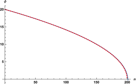
Explicit numerical evolution confirms these expectations. Figure 3 compares evolution for the classical and quantum systems with the small coupling of .


Because this particular model of classical inflation has , the parameter times on which the functions and depend is always in the large field regime,
| (29) |
Hence the quartic large field limit (12) of the quantum correction is valid throughout inflation, which makes the quantum correction less and less important as the scalar rolls towards zero.
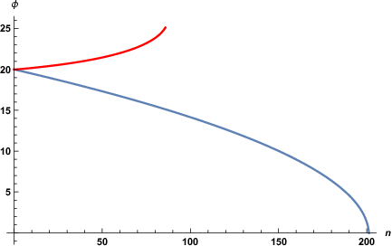


On the other hand, the slightly larger value of leads to the disastrous evolution shown in Figure 4. The fact that is driven to zero, while grows, increases the validity of the large field form (12), and makes the classical contribution ever less significant.
Figure 5 compares the initial shapes of the total potential for and for . We numerically checked that the large field estimate (28) of in fact marks the crossover point between the two regimes. Note that, whereas the large field limiting form (12) is independent of the classical potential, the threshold value of the coupling constant can be very different for different classical models. In particular, the very flat potentials favored by current data [21] correspond to much smaller values of .


4 Conclusions
Cosmological Coleman-Weinberg potentials are the price scalar-driven inflation pays for efficiently communicating the kinetic energy of the inflaton to ordinary matter. Although they take the same form as their famous flat space antecedents [9], explicit results on de Sitter background take the form of times very complicated functions of [16, 17]. A recent computation [12] strongly supports the idea that de Sitter results remain approximately valid when the constant Hubble parameter of de Sitter is replaced by the evolving of realistic inflation. The conundrum for scalar-driven inflation is that cosmological Coleman-Weinberg potentials are too large and too steep for successful inflation [10], while the degree to which they can be subtracted off using local, lower derivative counterterms is limited by their dependence on the Hubble parameter [11]. Unacceptable results follow from subtractions involving just the inflaton [13], or the inflaton and the Ricci scalar [14]. This paper has been devoted to a different approach in which no subtractions are made but one attempts instead to cancel the positive potentials induced by bosons with the negative potentials induced by fermions.
In section 2.1 we reviewed the effective potential (6-8) induced for a model (2) in which a complex scalar inflaton is coupled to fermions (with Yukawa constant ) and to vector bosons (with charge ). Choosing makes the positive large field form induced by vector bosons cancel the negative large field form induced by fermions. Unfortunately, the residual (16) is negative and still large enough to overwhelm classical inflation and make the universe suffer a Big Rip singularity unless the coupling constant is chosen smaller than the minuscule value of . Figures 3 and 4 show what happens for couplings below and above this critical value.
The ultimate problem with our cancellation scheme is that the cosmological Coleman-Weinberg potentials induced by different sorts of particles are all slightly different on the background of an expanding universe, even though they have the same functional form (up to a sign) on flat space background. Despite the unsatisfactory nature of our results so far we believe there is hope for a better outcome from two modifications. The first is to make a different choice for the finite part of the quartic counterterm (5) so as to cancel the term (12) of the residual result. In that case the leading large field behavior would go like , and the positive bosonic contribution should dominate the negative fermionic contribution. This residual should still be larger than the classical potential unless is very small, so one would need to worry about unacceptable large contributions to the power spectrum. Another concern is that the original counterterms (4-5) were chosen to keep the small field expansions of the effective potential weak so as not to disrupt late time physics [11].
An even more hopeful modification is to involve scalars in the cancellation scheme. In addition to its coupling with the inflaton, a real scalar possess an additional parameter characterizing its coupling to the Ricci scalar,
| (30) |
We can use this extra parameter to vary the results. If the renormalization constants are chosen according to the same scheme [11] that was used for fermions and vector bosons the resulting effective potential takes the form,
| (31) |
where . The function is [11],
| (32) | |||||
By employing a number of scalars with different values of and it may be possible to cancel enough terms in the large field expansion to make the residual harmless for at least some models of inflation.
Before closing we should comment on the specious argument sometimes advanced to dismiss the possibility that cosmological Coleman-Weinberg potentials pose any danger for inflation. The argument begins by observing that the inflaton is large during the early stages of inflation, endowing the ordinary matter to which it is coupled with a large mass. Of course that is correct, but the second part of the argument mistakenly concludes that such a large mass suppresses quantum fluctuations of ordinary matter so that they cannot make significant corrections to the effective potential. This reasoning is belied by the classic flat space results which are known to go like [9]. In fact the argument reveals a confusion about what the effective potential represents. At one loop order the primitive, unrenormalized, effective potential is just the integral of the 0-point energies from each plane wave mode ,
| (33) |
In flat space , so increasing the mass must increase, not decrease, the effective potential. This is evident if we perform the flat space computation with a momentum cutoff,
| (34) | |||||
| (35) | |||||
The primitive contribution (35) is renormalized by a counterterm with scale ,
| (36) |
Adding the counterterm (36) and taking the unregulated limit gives the familiar result [9],
| (37) |
From the integral (35) we can even see that the largest part of the final answer (37) derives from momenta up to , so large values of result in high momentum modes contributing. The expansion of the universe changes the analysis in important ways, but it does not alter the basic fact that increasing the inflaton field strength, which increases , increases the effective potential that is induced. Note also that increasing does suppress the length of time virtual particles can persist, so it really does suppress many other quantum effects, just not the effective potential.
Acknowledgements
This work was partially supported by Taiwan MOST grants 108-2112-M-006-004 and 107-2119-M-006-014; by NSF grants PHY-1806218 and PHY-1912484; and by the Institute for Fundamental Theory at the University of Florida.
5 Appendix: Hubble Proxies
Although loop contributions to the effective action are not generally local, any subtraction of them must be local, generally coordinate invariant, and free of the instabilities that plague interacting continuum field theories which contain nondegenerate higher time derivatives [15]. In short, any subtraction must be acceptable as part of the classical action. One cannot otherwise compute inflationary perturbations, and couple inflation to ordinary matter.
The Hubble parameter which characterizes cosmological expansion is not a local, generally coordinate invariant functional of the metric. Any subtraction scheme that attempts to exactly cancel cosmological Coleman-Weinberg potentials must exploit a proxy for the Hubble parameter, that is, an invariant functional of fields which reduces to in the homogeneous and isotropic geometry (3) of an expanding universe. The usual technique for constructing such a proxy is based on taking the divergence of a normalized, timelike vector field [22],
| (38) |
The question then becomes, where are we to find the normalized, timelike vector field ? The literature provides three sorts of answers:
Each of the three Hubble proxies has problems associated with the fact that it is fundamentally some functional of fields which only reduces to the Hubble parameter after the equations of motion are used and the geometry is specialized to (3). Hence the variations that give the field equations (which must be taken before specialization) can introduce undesirable effects. For example, constructing the timelike vector from the gradient of the inflaton obviously involves higher time derivatives (and hence Ostrogradsky instabilities) when (39) is substituted in (38). The 2nd construction is unacceptable because the Hubble proxy is not even a local functional of the metric. The 3rd construction will see variations of the Hubble proxy making extensive changes in the field equation. Even if these changes should prove benign, it is known that cosmological Coleman-Weinberg potentials depend in a complicated way on the first slow roll parameter , in addition to just the Hubble parameter [12]. Attempting to include this dependence will introduce higher time derivatives of , which must engender Ostrogradsky instabilities.
References
- [1] G. Geshnizjani, W. H. Kinney and A. Moradinezhad Dizgah, JCAP 11 (2011), 049 doi:10.1088/1475-7516/2011/11/049 [arXiv:1107.1241 [astro-ph.CO]].
- [2] W. H. Kinney, G. Geshnizjani and A. Moradinezhad Dizgah, “Inflation, Or What?,” in 47th Rencontres de Moriond on Cosmology: La Thuile, Italy, March 10-17, 2012, ed. E. Augé, J. Dumarchez and J. T. T. Van, pp. 179-184.
- [3] Y. Akrami et al. [Planck Collaboration], arXiv:1807.06211 [astro-ph.CO].
- [4] A. Ijjas, P. J. Steinhardt and A. Loeb, Phys. Lett. B 723, 261 (2013) doi:10.1016/j.physletb.2013.05.023 [arXiv:1304.2785 [astro-ph.CO]].
- [5] A. H. Guth, D. I. Kaiser and Y. Nomura, Phys. Lett. B 733, 112 (2014) doi:10.1016/j.physletb.2014.03.020 [arXiv:1312.7619 [astro-ph.CO]].
- [6] A. Linde, doi:10.1093/acprof:oso/9780198728856.003.0006 arXiv:1402.0526 [hep-th].
- [7] A. H. Guth et al. [33 co-authors], “A Cosmic Controversy,” (Letter to the Editor), Scientific American (May 10, 2017).
- [8] A. Ijjas, P. J. Steinhardt and A. Loeb, Phys. Lett. B 736, 142 (2014) doi:10.1016/j.physletb.2014.07.012 [arXiv:1402.6980 [astro-ph.CO]].
- [9] S. R. Coleman and E. J. Weinberg, Phys. Rev. D 7, 1888 (1973). doi:10.1103/PhysRevD.7.1888
- [10] D. R. Green, Phys. Rev. D 76, 103504 (2007) doi:10.1103/PhysRevD.76.103504 [arXiv:0707.3832 [hep-th]].
- [11] S. P. Miao and R. P. Woodard, JCAP 1509, 022 (2015) doi:10.1088/1475-7516/2015/09/022, 10.1088/1475-7516/2015/9/022 [arXiv:1506.07306 [astro-ph.CO]].
- [12] A. Kyriazis, S. P. Miao, N. C. Tsamis and R. P. Woodard, arXiv:1908.03814 [gr-qc].
- [13] J. H. Liao, S. P. Miao and R. P. Woodard, Phys. Rev. D 99, no. 10, 103522 (2019) doi:10.1103/PhysRevD.99.103522 [arXiv:1806.02533 [gr-qc]].
- [14] S. P. Miao, S. Park and R. P. Woodard, Phys. Rev. D 100, no. 10, 103503 (2019) doi:10.1103/PhysRevD.100.103503 [arXiv:1908.05558 [gr-qc]].
- [15] R. P. Woodard, Lect. Notes Phys. 720, 403 (2007) doi:10.1007/978-3-540-71013-4_14 [astro-ph/0601672].
- [16] P. Candelas and D. J. Raine, Phys. Rev. D 12, 965 (1975). doi:10.1103/PhysRevD.12.965
- [17] B. Allen, Nucl. Phys. B 226, 228 (1983). doi:10.1016/0550-3213(83)90470-4
- [18] S. P. Miao and R. P. Woodard, Phys. Rev. D 74, 044019 (2006) doi:10.1103/PhysRevD.74.044019 [gr-qc/0602110].
- [19] T. Prokopec, N. C. Tsamis and R. P. Woodard, Annals Phys. 323, 1324 (2008) doi:10.1016/j.aop.2007.08.008 [arXiv:0707.0847 [gr-qc]].
- [20] J. Z. Simon, Phys. Rev. D 41, 3720 (1990). doi:10.1103/PhysRevD.41.3720
- [21] N. Aghanim et al. [Planck Collaboration], arXiv:1807.06209 [astro-ph.CO].
- [22] G. Geshnizjani and R. Brandenberger, Phys. Rev. D 66, 123507 (2002) doi:10.1103/PhysRevD.66.123507 [arXiv:gr-qc/0204074 [gr-qc]].
- [23] S. Miao, N. Tsamis and R. Woodard, Phys. Rev. D 95, no.12, 125008 (2017) doi:10.1103/PhysRevD.95.125008 [arXiv:1702.05694 [gr-qc]].
- [24] T. Jacobson and D. Mattingly, Phys. Rev. D 64, 024028 (2001) doi:10.1103/PhysRevD.64.024028 [arXiv:gr-qc/0007031 [gr-qc]].