Efficient Nonnegative Tensor Factorization via Saturating Coordinate DescentJournal: TKDDVolume: 1111Price: 15.00DOI: 10.1145/3385654CCS: Computing methodologies Factorization methodsCCS: Information systems Recommender systemsCCS: Information systems Spatial-temporal systemsCCS: Theory of computation Nonconvex optimization
Abstract.
With the advancements in computing technology and web-based applications, data is increasingly generated in multi-dimensional form. This data is usually sparse due to the presence of a large number of users and fewer user interactions. To deal with this, the Nonnegative Tensor Factorization (NTF) based methods have been widely used. However existing factorization algorithms are not suitable to process in all three conditions of size, density, and rank of the tensor. Consequently, their applicability becomes limited. In this paper, we propose a novel fast and efficient NTF algorithm using the element selection approach. We calculate the element importance using Lipschitz continuity and propose a saturation point based element selection method that chooses a set of elements column-wise for updating to solve the optimization problem. Empirical analysis reveals that the proposed algorithm is scalable in terms of tensor size, density, and rank in comparison to the relevant state-of-the-art algorithms.
Keywords:
Nonnegative Tensor Factorization, Coordinate Descent, Element selection, Saturating Coordinate Descent, Pattern Mining, Recommender systems1. Introduction
With the advent of tagging, sensor and Internet of Things (IoT) technologies, online interaction data can be easily generated with tagging or spatio-temporal information. Tensor models become the natural choice to represent a multi-dimensional dataset, for example as ( ) or ( ) (Ifada and Nayak 2014; Kolda and Bader 2009; Symeonidis 2016; Balasubramaniam et al. 2019). A Tensor Factorization (TF) based method decomposes the tensor model into multiple factor matrices where each matrix learns the latent features inherent in the usage dataset (Kolda and Bader 2009; Zheng et al. 2014). These factor matrices can be used to reconstruct (or approximate) the tensor to predict missing entries. These entries can be inferred as new items that have been generated based on correlations and dependencies between the data, and help in making recommendation generation and link prediction (Rendle and Schmidt-Thieme 2010; Dunlavy et al. 2011; Ermiş et al. 2015; Adomavicius and Tuzhilin 2005). A learned factor matrix reveals the latent features that are able to represent hidden patterns in the dataset in that particular dimension, and can help to understand people’s mobility patterns and usage (Symeonidis et al. 2013).
A TF process is challenging for three main reasons. Firstly, a tensor model tends to grow big as the data size increases. It especially becomes a problem for web applications due to a large Internet population and fewer user interactions. Secondly, due to fewer user interactions with all the items, the data generated is very sparse. Learning the associations or analyzing this sparse dataset is hard due to lack of correlation patterns. Thirdly, the complexity of factorization process increases with an increase in the rank of the tensor. Here, the rank represents the number of hidden features in the dataset, in other words, it decides the size of factor matrices. Computing a large size sparse tensor model for exploring hidden latent relationships in the dataset is still a challenging problem. Table 1 shows the limited scalability of existing factorization algorithms. Nonnegative Tensor Factorization (NTF) which imposes the nonnegative constraint to the factor matrices learned during factorization is the backbone of recommendation and pattern mining methods to understand interactions between features. The development of a fast and efficient NTF algorithm is needed for developing effective web recommendation and pattern mining methods.
We propose the Saturating Coordinate Descent (SaCD) factorization algorithm that reduces the complexity inherent in the factor matrix update by carefully selecting the important elements to be updated in each iteration. We propose a Lipschitz continuity based element importance calculation to effectively select the elements for an update that will lead fast convergence. We also propose a fast-parallelized version of SaCD (named as FSaCD) to further speed up the factorization process that suffers from Intermediate Data Explosion (IDE). IDE is caused due to the materialization and storage of the intermediate data generated. The column-wise element selection and element update minimizes the complexity of IDE and parallelization becomes easier.
Extensive experiments with recommendation and pattern mining applications show improved scalability (i.e. size, density and rank) performance of SaCD and FSaCD in comparison to all relevant baseline algorithms. The results also show that the efficiency is achieved at no cost of accuracy. In fact, SaCD achieves high accuracy when compared to other benchmarks.
| Algorithm | Mode length | Density | Rank |
|---|---|---|---|
| APG (Zhang et al. 2016) | Low | Low | Low |
| FMU (Phan et al. 2012) | Medium | Low | Medium |
| FHALS (Phan et al. 2013) | Medium | Low | Medium |
| BCDP (Xu and Yin 2013) | Medium | Medium | High |
| CDTF (Shin et al. 2017) | High | Medium | Low |
| GCD (Balasubramaniam et al. 2018a) | High | Medium | Low |
| SaCD | High | High | High |
| FSaCD | High | Very High | High |
The specific contribution of this paper is four-fold.
- (1)
We propose a novel Lipschitz continuity based element importance calculation method to select certain elements for updating in the factorization process.
- (2)
We propose a novel Saturating Coordinate Descent (SaCD) factorization algorithm that updates factor matrices by selecting elements using the proposed Lipschitz continuity based element importance and leads fast convergence to a local optimum solution.
- (3)
We apply SaCD in recommender systems and pattern mining effectively with high accuracy and scalability.
- (4)
We design FSaCD by parallelizing SaCD on the single machine using multi-cores that further improves the performance on big and dense datasets.
To our best of knowledge, SaCD is the first algorithm that can efficiently process the large and sparse tensor model with large rank factor matrices, with and without parallelization.
2. Related Work
Tensor Factorization based recommender systems and pattern mining methods: Tensor models have been widely applied in several web-based applications and have shown superiority in generating latent patterns (Ifada and Nayak 2016; Ermiş et al. 2015; Sun and Axhausen 2016). The majority of model-based Collaborative Filtering methods, including Matrix Factorization (MF), fail to utilize a context along with users and items information because of their limited capability to deal with two-dimensional data only (Symeonidis 2016). The capability of a tensor model to represent multidimensional data makes them a natural choice to represent the user interaction data (Kutty et al. 2012). The last decade has witnessed the rise of tensor-based recommendation methods (Ifada and Nayak 2014; Symeonidis 2016; Yu and Chen 2015; Zheng et al. 2010; Symeonidis et al. 2008; Rendle and Schmidt-Thieme 2010).
A three dimensional tensor model represents the data as ( ) and a tensor factorization (TF/NTF) algorithm can be used to capture dimensional dependencies and general recommendations (Karatzoglou et al. 2010). For example, a ( ) tensor model has been used in social tagging systems for representing how users have used tags with items (Bouadjenek et al. 2016; Ifada and Nayak 2016). A TF method with higher order singular value decomposition (HOSVD) has been used to recommend items based on tagging behavior or to recommend tags for items (Symeonidis et al. 2009). Link prediction in social networks has been solved using Alternating Least Square (ALS) based NTF by predicting the missing relations in the dataset, for example, identifying relations among users or recommending items to users by considering time as the additional context (Ermiş et al. 2015). Researchers have used the approach to minimize the size and sparsity of the tensor by only including the data with occurrence of (user, item) at least times, as the traditional TF/NTF methods are not scalable and their accuracy on the sparse dataset is low (Ifada and Nayak 2016; Rendle and Schmidt-Thieme 2010; Balasubramaniam et al. 2019). However, the approach removes any users/items with less than interactions, thus, leaving the recommendation process incomplete for some users.
Recent advancements in IoT allow recording additional spatio-temporal information easily in addition to the web interactions. This has led to focus research on Location-Based Social Networks (LBSNs) (Yu and Chen 2015). Researchers have successfully applied TF/NTF using ALS for automated mining of temporal patterns (Balasubramaniam et al. 2018a; Liu and Xiong 2013). For example, the Foursquare dataset with the user, venue and time is represented as a tensor and the number of patterns are identified by the factor matrix in the time mode where is a tensor rank (Zheng et al. 2014). Similarly, the temporal trajectories of online gamers are derived using NTF (Sapienza et al. 2018). These patterns allow learning the behavior of web users that helps to personalize and improve the interactions. Tensor rank is an important parameter in the factorization process that learns the hidden features of the dataset. These hidden features represent the data effectively in a lower dimension, where higher the number of hidden feature identified, higher is the chances of learning the true representation of dataset (Symeonidis 2016).
With the dependence of these methods on TF to learn the associations in the data, it is important that a factorization algorithm can efficiently deal the tensor models with the larger size, density, and rank.
Fast Tensor Factorization Algorithms: Factorization algorithms namely Alternating Least Square (ALS) [23], Multiplicative Update rule (MU) (Cichocki et al. 2009), Gradient Descent (GD) (Zhang et al. 2016) and Coordinate Descent (CD) (Hsieh and Dhillon 2011; Wright 2015; Nesterov 2012) have been commonly used to factorize the tensor models. These traditional algorithms have been extended to tensors based on MF. Researchers have explored the concepts of gradient calculation and tensor block to fasten the factorization process in these factorization algorithms. Fast Hierarchical ALS (FHALS) (Phan et al. 2013) and Fast MU (FMU) (Phan et al. 2012) are the optimized variants of ALS and MU by exploiting an efficient gradient calculation method for the faster execution. The traditional gradient calculation requires the tensor unfolding at each iteration which is relatively slow. FHALS and FMU use a simplified update rule with the gradient calculation that does not require the tensor unfolding. Accelerated Proximal Gradient (APG) (Zhang et al. 2016) utilizes a low-rank approximation to speed up the factorization process. The Block Coordinate Descent (BCDP) (Xu and Yin 2013) technique has been applied in NTF to minimize the complexity by processing the tensor in convex blocks. The element selection-based CD algorithm called Greedy Coordinate Decent (GCD) (Hsieh and Dhillon 2011) has shown fast convergence in Nonnegative Matrix Factorization (NMF) process. But the extension of GCD to NTF involves high complexity because of the frequent gradient updates (Balasubramaniam et al. 2018a).
Few researchers have explored parallel and distributed computational methods to minimize the time complexity involved in the Matricized Tensor Times khatri-Rao Product () and matrics updates during TF (Shin et al. 2017; Oh et al. 2017; Kang et al. 2012; Choi and Vishwanathan 2014; Beutel et al. 2014; Park et al. 2016; Smith et al. 2015). CCD++ (Yu et al. 2012) is a CD algorithm for MF that updates the elements in a factor matrix column-wise. Coordinate Descent for Tensor Factorization (CDTF) (Shin et al. 2017) and Subset Alternating Least Square (SALS) (Shin and Kang 2014) are two recent extensions of CCD++ for TF. While CDTF is a direct extension of CCD++ for TF, SALS is a special case with an additional constraint that controls the number of columns to update in a single iteration. The column-wise factor matrix update minimizes the complexity of in these algorithms and introduces a huge advantage in the distributed and parallel environment. However, these implementations do not alter the computational complexity inherent in the underlying factorization algorithm. We have implemented CDTF for NTF and used it as a benchmark in experiments. SALS cannot be directly extended for NTF due to the additional constraint it imposes.
Limitations: While NTF has been applied widely with tensor based methods to utilize multi-dimensional data, it suffers from the scalability issue due to the complex matrix and tensor products involved in the factorization process (Shin et al. 2017). Existing factorization algorithms are limited to small datasets only (as listed in Table 1). While parallel and distributed computational methods improve the runtime and scalability by utilizing huge resources, performance on a normal machine with fewer memory requirements remains poor (Oh et al. 2017). While optimizing the basic factorization process can improve the performance without depending on huge resources, not all the optimized factorization algorithms are easily extendable to a parallel and distributed environment to further improve the performance (Kimura and Kudo 2015). Most importantly, not all the factorization algorithms can effectively handle tensors of large size, sparsity, and rank (Oh et al. 2017). We propose a factorization algorithm, SaCD, to efficiently process the large and sparse tensor model, with and without parallelization, by avoiding the frequent gradient calculations that are essential in existing algorithms (Hsieh and Dhillon 2011; Balasubramaniam et al. 2018a).
3. Basics: Preliminaries and Definitions
The notations used in this paper are summarized in Table 2. The process of converting a tensor into a matrix is called as matricization or unfolding of tensor (Tucker 1966). The matricization can be denoted as for a third order tensor where , , and denotes the mode length. Several matrix products are required for tensor-based processes (Lathauwer 2008). We briefly introduce them.
| Symbol | Definition |
|---|---|
| tensor (Euler script letter) | |
| 3 modes of | |
| Length of mode respectively | |
| set of indices of observable entries of | |
| entry of | |
| subset of whose mode ’s index is | |
| subset of whose mode ’s index is | |
| subset of whose mode ’s index is | |
| matrix (upper case. bold letter) | |
| vector (lower case, bold letter) | |
| scalar (lower case, italic letter) / element | |
| mode-n matricization of tensor | |
| rank of tensor | |
| Kronecher product | |
| Khatri-Rao product | |
| Hadamard product | |
| outer product | |
| Frobenius norm |
3.1. Kronecker Product
For two matrices denoted as and , the Kronecker product is presented as . The resultant matrix of size is defined as follows:
| (1) |
| (2) |
where is column of the factor matrix .
3.2. Khatri-Rao Product
The column-wise Kronecker product, called as Khatri-Rao product, is denoted as . The resultant matrix of size is defined as:
| (3) |
where and are columns of the matrices and respectively.
3.3. Hadamard Product
When the size of two matrices are same, the hadamard product can be calculated by the element-wise matrix product. It is denoted by and defined as:
| (4) |
3.4. Tensor Factorization
Tensor factorization, a dimensionality reduction technique, is an extension of matrix factorization for higher order. It factorizes a tensor into factor matrices that contain latent features. CANDECOMP/PARAFAC (CP) and Tucker are two well-known factorization techniques (Kolda and Bader 2009). CP has shown to be less expensive in both memory and time as compared to Tucker (Oh et al. 2017; Kolda and Bader 2009).
Definition 1 (CP Factorization): For a tensor and rank , CP factorization factorizes the tensor into a sum of component rank-one tensors (Carroll and Chang 1970) (as shown in Figure 1) as:
| (5) |
where , and are factor matrices with hidden features, .
The goal of CP tensor factorization is to approximate the input tensor and its objective function can be formulated as follows,

| (6) |
The learning process is modeled as the minimization of Euclidean loss function as shown in Equation (6). The optimization process (Equation (7)) aims to learn the factors to reduce the difference between the original tensor and approximated tensor, where the predicted value is calculated by the inner product of learned factors across all the features, as formulated in Equation (8) (Cichocki et al. 2009):
| (7) |
| (8) |
3.5. Nonnegative Tensor Factorization (NTF)
The basic idea of NTF is factorizing the -dimensional tensor into factor matrices that satisfy the nonnegative constraint (Kolda and Bader 2009). NTF can be achieved in traditional Tucker or CP factorization model by imposing constraints to maintain the nonnegative values.
The objective function for NTF based on CP model can be formulated as follows:
| (9) |
The approximated tensor, after factorization, using the learned factor matrices will be a denser model in which a large portion of absent values are populated (Nguyen and Ho 2016; Sra et al. 2008). For applications such as predictive modelling and recommender systems, these populated values can be inferred as potential prediction or recommendation (Ifada and Nayak 2014; Balasubramaniam et al. 2018b).
The goal of the optimization problem in Equation (9) is to find the accurate factor matrices , and . ALS (Takane et al. 1977) is the most common algorithm used to find the factor matrices (Sidiropoulos et al. 2017; Phan et al. 2013). It gives equal importance to all the elements and alternatively updates the entire factor matrix by fixing all the other factor matrices. This unnecessary element updates can cause slow convergence and poor scalability (Acar et al. 2011; Hsieh and Dhillon 2011).
4. Saturating Coordinate Descent Algorithm for NTF
In this paper, we propose the Saturating Coordinate Descent (SaCD) algorithm to solve Equation (9) in order to reduce the complexity inherent in the factor matrix update and to overcome the poor scalability faced by traditional algorithms like ALS (Phan et al. 2013), APG (Zhang et al. 2016), GCD (Hsieh and Dhillon 2011), CDTF (Shin et al. 2017) and BCDP (Xu and Yin 2013). Figure 2 provides the detail of the overall process.
4.1. Factor Matrix Update Rule
We First explain the learning process of factor matrix which is applicable to other factor matrices. The factor matrix is updated by solving Equation (10) and to solve, we need to find the first order and second partial derivatives (Equation (11) and Equation (12) respectively) for in Equation (9) as follows,
| (10) |
| (11) |
| (12) |
where and are the first order and second order partial derivatives of the objective function (Equation (9)) with respect to and let us denote them as (gradient) and (second order derivative) respectively.
The one variable gradient and second order derivative are computed as,
| (13) |
| (14) |
where and represents and gradient and second order derivative respectively.
Equation (9) becomes a quadratic equation in terms of the updated parameter when all other parameters are fixed. This leads to the following closed form CD update rule (i.e., one variable sub-problem) (Phan et al. 2013) for each parameter:
| (15) |
The one variable sub-problem can be a simplified ALS update rule where each factor matrix is updated element-wise, thus it reduces the computational complexity. The nonnegative constraint can be added to Equation (15) as,
| (16) |
where indicates the element of the factor matrix and indicates the computed element.
With the computed element value (), the element can be updated as,
| (17) |
Since the calculation of and for every element is expensive, it is better to calculate this value only once at each iteration, instead of calculating it for every element update, during the factorization process to find the best learning factor matrices.
In NMF, element selection has been proven to converge faster for updating the important elements repeatedly, instead of considering all elements (Hsieh and Dhillon 2011). The traditional measurement of element importance and update is computationally inefficient for NTF due to frequent gradient updates. Next, we show how an element importance can be efficiently calculated and only important elements can be updated that can avoid frequent gradient updates.
4.2. Proposed Lipschitz Element Importance
The existing partial differential equations based optimization algorithms like APG, FHALS, FMU, and GCD are prone to slow convergence due to inconsistent gradients, i.e., gradients shift on both directions from the global or local minima in the non-convex optimization curve (Khamaru and Wainwright 2018). Additional regularity conditions has been incorporated to speed-up the convergence in NMF (Guan et al. 2012). In this paper, we propose to smooth (Lipschitz smoothness) the continuous function with a strong condition of Lipschitz continuity for fast convergence.
Definition 2 (Lipschitz continuity): Lipschitz continuity is a strong form of uniform continuity for a function if the function is differentiable with Lipschitz constant .
The continuously differentiable function is called Lipschitz continuous with Lipschitz constant , such that:
| (18) |
where and are two factor matrices at two consecutive iterations.
Definition 3 (Lipschitz smoothness): The Lipschitz continuous function, as defined in Equation (18), can be smoothed with the upper bound value for . It ensures the strong convexity of the function and achieves faster convergence. This property is called Lipschitz smoothness and the function with this property is called -smoothed. It can be defined as,
| (19) |
The upper bound value for should be calculated to satisfy,
| (20) |
where is an Identity matrix.
Equations (11) and (12) can reveal that the objective function is differentiable with respect to factor matrices as well as it is non-convex. We propose to analyse these properties using Lipschitz continuity and Lipschitz smoothness and measure the element importance in order to achieve faster convergence.
Let be the element importance matrix that holds the importance value for each element in a factor matrix. The importance of element can be calculated as the difference in the objective function as,
| (21) |
where represents the gradient of and represents the new gradient value of the computed element .
With the precomputed as per Equation (13), we can compute using one variable subproblem (Hsieh and Dhillon 2011) as follows,
| (22) |
In Equation (23), is the partial derivative of gradient as defined in Equation (14). An objective function holding Lipschitz continuity with differentiable gradients can be Lipschitz-smoothed (-smoothed) (as proven in Lemma 4.1). This property will allow the function to converge faster by replacing the partial derivative of gradient (i.e. in (23)) with Lipschitz constant (Guan et al. 2012).
We propose to calculate the difference in the -smoothed objective function for each element’s update during the factorization using Lipschitz continuity (Hager 1979) that can achieve faster convergence. The convergence of an optimization problem can be analyzed using curvature measure that measures the deviation of the objective function with the linear approximation. The Lipschitz smoothness of has shown the best with the improvement of convergence speed to where is the number of iterations (Jaggi 2011) 11 1 For a formal analysis of curvature measure and Lipschitz continuity, we direct the readers to (Jaggi 2011).. We conjecture that use of Lipschitz continuity in the element importance calculation will speed up the convergence.
By applying the upper bound value of Lipschitz continuity in the one variable subproblem Equation (22), we have:
| (24) |
where is a positive scalar called Lipschitz constant.
With the redefined one variable subproblem, we can define Lipschitz element importance by substituting Equations (13) and (24) in Equation (21) as,
| (25) |
Lemma 4.1.
The gradient of the objective function Equation (9) satisfies Lipschitz continuity.
Proof.
Supposedly we have two factor matrices and at two consecutive iterations.
| (26) |
Applying Definition 2 and assuming the objective function is differentiable, we obtain,
| (27) |
4.3. SaCD (Saturating Coordinate Descent)
Once we have the element importance calculated for all the elements in the factor matrix using Equation (25) and stored them in , we now select a set of elements for every iteration using the proposed SaCD algorithm. The state-of-the-art GCD NMF algorithm uses greedy strategy in finding and updating single element multiple times in each row (Hsieh and Dhillon 2011). This requires a very expensive frequent gradient update. In the minimization optimization problem as formulated in Equation (9), the error is minimized for each iteration. It slowly reaches convergence, or reaches a saturation point beyond which updating will not minimize the objective function . Hence, the contribution of each element in minimizing the objective function decreases with each iteration. Moreover, not all the elements will effectively minimize the objective function. It is sufficient and efficient to update every single element until it reaches the saturation point, instead of updating it for all the iterations. This avoids the expensive frequent gradient update as proven in Lemma 4.2.
As the element importance is the difference in the objective function as per Equation (21), we can identify the saturation point of each element for every iteration , by keeping track of the previous value of as,
| (28) |
Additionally, for each iteration, we measure the total importance of a factor matrix as,
| (29) |
| (30) |
If the total importance of current iteration is more than the previous iteration , we identify the saturation point as,
| (31) |
While the difference in the objective function gradually decreases, sometimes it increases. This happens when the optimization is reaching local or global minima. To avoid stuck in local minima, this redefinition of the saturation point is needed that further allows important elements to be updated until global minima is reached. We use this saturation point to decide if the element is to be updated as per Equation (17). If , we avoid updating that element.
We have explained the proposed algorithm by describing the learning process of factor matrix . Next we briefly show that the process is applicable to other factor matrices too.
Lemma 4.2.
In the SaCD element selection, for each update of , it is not necessary to update gradient of all the columns of row and element importance .
Proof.
Let be element of and represents gradient of .
For every , the set of important elements are selected based on the saturation point calculated using Equation (28) or Equation (31).
The subset is dependent on column of .
For each update of alone needs to be updated as where and where and indicates that is independent of .
Therefore, for each update of , it is enough to update alone and it is not necessary to update of all the columns of row and element importance .
∎
Updating solution for factor matrix :
Taking the first and second order partial derivatives of the function with respect to , we have a new solution for the gradient and second order derivative as,
| (32) |
| (33) |
Updating solution for factor matrix :
Taking the first and second order partial derivatives of the function with respect to , we have a new solution for the gradient and second order derivative as,
| (34) |
| (35) |
With the updated and as per Equations (34) and (35), the element importance is calculated according to Section 4.1 and the factor matrix update is performed in similar fashion.
Algorithm 1 details the process.
Output: Learned Factor matrices , ,
for do 1
identify the saturation point using Equation (28) or Equation (31);
if then 13
repeat analogues lines 4 to 26 with and calculated using Equations (34) and (35) respectively to update elements of in lines 11 and 21;
end for 18
4.4. Fast Saturating Coordinate Descent (FSaCD) using Parallelization
In this section we propose the Fast SaCD algorithm that leverages the column-wise element update to speed up the factorization process of SaCD. Instead of pre-computing the gradient using Equation (11), we propose to calculate the gradient column-wise during the column-wise element update. To further improve the performance of SaCD, we utilize the multiple cores of the single machine.
The pre-calculation of as per Equation (11) consists of an expensive operation (i.e., ), a complex step in factorization that causes the Intermediate Data Explosion (IDE). IDE is caused due to the materialization and storage of the intermediate data (). The calculation of is a rather infamous computational kernel with a lot of related work attempting to optimize the computations (Smith et al. 2015; Choi and Vishwanathan 2014; Bader and Kolda 2007). We utilize the concept of sparse tensor times vector product () which redesigns the NTF algorithm to calculate the column-wise (Bader et al. 2017). simplifies by multiplying sparse tensor to a vector instead of multiplying it to a matrix and minimizes the IDE. We call this Fast SaCD algorithm as FSaCD. We propose to calculate the element importance and column-wise and parallelize the calculation together.
Based on Algorithm 1, we calculate the element importance column-wise so that only the respective column of gradients is needed. It enables us to calculate the of only one column at a time as follows,
For simplicity, let us represent as,
| (36) |
The operation is simplified using the sparseness of tensor and the column-wise () can be calculated as,
| (37) |
where indicates a subset of whose mode ’s index is . and indicates the column of the factor matrices and respectively.
Now, the column-wise gradient to solve is calculated as,
| (38) |
The column-wise element importance is calculated as,
| (39) |
With the calculated gradient (Equation (38)) and element importance (Equation (39)), the column-wise update is performed as,
| (40) |
where indicates the column of the factor matrix and .
The above process shows the learning of factor matrix . Next we briefly show that the process is applicable to other factor matrices and too.
Updating solution for factor matrix :
The () operation in Equation (32) can be calculated column-wise as,
| (41) |
Now, the column-wise gradient to solve is computed as,
| (42) |
The column-wise element importance is calculated as,
| (43) |
Updating solution for factor matrix :
The () operation in Equation (34) can be calculated column-wise as,
| (45) |
Now, the column-wise gradient to solve is computed as,
| (46) |
The column-wise element importance is calculated as,
| (47) |
With the calculated gradient (Equation (46)) and element importance (Equation (47)), the column-wise update is performed as,
| (48) |
where indicates the column of the factor matrix and .
With the column-wise gradients calculated as per Equations (38), (42), and (46), and the column-wise element importance calculated as per Equations (39), (43), and (47), the factor matrix update is performed in parallel as detailed in the Algorithm 2.
Output: Learned Factor matrices , ,
for do 1
compute element importance using Equation (39);
store the initial element importance, ;
if then 4
repeat analogues lines 4 to 26 with , and calculated using (35), (46) and (47) respectively to update the elements of in lines 11 and 21;
end for 16
5. Theoretical Analysis
We analyze SaCD in terms of convergence, time complexity, and memory requirement. We use the following symbols in the analysis: (rank), (maximum number of iterations), (number of factor matrices, and a three-mode tensor .
5.1. Convergence Analysis
In this section, we analyze the convergence of SaCD under the following assumptions.
Assumption 1. The objective function w.r.t each factor matrix is continuous, differentiable and holds the Lipschitz continuity.
Assumption 2. Each element importance is calculated by Equation (25) for all iterations and the parameter obeys .
Lemma 5.1.
Based on the and , for given iterations, .
Proof.
For the element selection as per Equation (28), we have inequality and therefore,
| (49) |
If we sum the above inequality over from to , we have
| (50) |
As the function is lower bounded, for , the proof satisfies. ∎
The update rule in Equation (22) utilizes the Newton method (Lee and Seung 2001) to apply the updates to the set of important elements that are identified by SaCD.
Theorem 5.2.
The newton method update rule using SaCD converges faster to the optimal solution by reaching the saturation point.
Proof.
The Newton method based update uses the update sequence,
| (51) |
where indicates the iteration. Using SaCD, we select where is a set of elements to be updated in . The gradients and second order derivatives for the sequence can be defined as:
| (52) |
| (53) |
As per linear differential equations properties, for any positive . As we know that , and setting , we have
| (54) |
With the initialized , suppose the update sequence that holds these properties will converge to a saturation point where . For the larger value of by continuity of given gradients and second-order derivatives,
| (55) |
| (56) |
5.2. Time Complexity
Lemma 5.3.
The time complexity of SaCD is
Proof.
Algorithm 1 includes five operations: initialization of factor matrices and respective importance matrix , unfolding of the tensor, gradient calculation, updating of factor matrices, and updating of importance matrix.
The random initialization of number of factor matrices and respective importance matrix takes . Unfolding the tensor generally takes . SaCD requires gradients to be calculated before updating the elements that involves the calculation of two terms and as shown in Equation (11) and Equation (13) and requires respectively. Let be the total number of elements selected for update. Updating each factor matrix takes and calculating takes additional , where . For each iteration, the value of reduces and at some point, it will reach . But if can be kept in memory, it can be updated while updating each entry for . Thus, the time complexity of SaCD can be formulated as . ∎
The time complexity of a third-order tensor factorization algorithms, including SaCD, remains to be cubical (). However, the element selection in SaCD avoids frequent element updates and controls the complexity as the number of element updates .
5.3. Memory Requirement
Lemma 5.4.
The memory requirement of SaCD is .
Proof.
For the factorization of an input tensor , SaCD stores the following types of data in the memory at each iteration: Unfolded tensor; Factor matrices and respective importance matrices; and precomputed gradient and second order derivative. The unfolded tensor with respective to any mode requires . The number of factor matrices require while the respective importance matrices require the same amount of memory . The precomputed gradients which is of the same size as the respective factor matrices will require another . The Hadamard matrix which is a square matrix for each factor matrix will require an additional memory. Thus, the memory requirement of SaCD is . ∎
6. Empirical Analysis
We would like to validate that SaCD can perform the factorization process efficietly as well as accurately. Experiments were conducted to answer the following questions:
Q1. How scalable is SaCD? What is its runtime performance?
Q2. How accurately can SaCD predict missing values and can be used in recommendation?
Q3. How accurately SaCD identify the unique patterns and can be used in pattern mining?
Q4. What is the impact of parallelization on SaCD?
6.1. Datasets
Several real-world and synthetic datasets were used to evaluate the performance of SaCD in comparison to the state-of-the-art algorithms. Table 3 details the four real-world datasets used. Delicious22 2 https://del.icio.us/ consists of user’s tagging behavior on 24073 URLs with tags. LastFM33 3 https://www.last.fm/ consists of users, artists and tags associated with the artists. Movielens44 4 https://movielens.org/ consists of , and user, movies and tags respectively. Gowalla55 5 http://www.yongliu.org/datasets/, the LBSN Foursquare dataset, records the users’ check-in activity at locations.
| Dataset | Tensor Size | Density |
|---|---|---|
| Delicious | ||
| LastFM | ||
| Movielens | ||
| Gowalla |
6.2. Experimental Setup and Benchmarks
The source codes of SaCD and its parallelized version have been made available66 6 https://github.com/thirubs/SaCD. All single-core experiments were executed on model with . The multi-cores experiments in section 6.4 were executed on model with and . For real-world datasets, we use fold cross validation with % of data used for training and % for testing.
We compare SaCD with the following benchmark algorithms.
- (1)
APG (Zhang et al. 2016) uses gradients to accelerate the convergence. The objective function is smoothed using the proximal gradients and the gradient calculation is simplified using the low-rank approximations. Instead of calculating the gradient using the original tensor , the low-rank approximations of the original tensor is used to calculate the gradients.
- (2)
FMU (Phan et al. 2012) and FHALS (Phan et al. 2013) are optimized variations of MU and ALS respectively. The tensor unfolding and the Kronecker product during the gradient calculations are simplified to minimize the computational cost.
- (3)
BCDP (Xu and Yin 2013) decomposes the non-convex optimization function into multiple blocks of convex problem. And the convex blocks are solved cyclically to update the factor matrices. The convex blocks are smoothed for fast convergence.
- (4)
CDTF (Shin et al. 2017) is a latest CD algorithm for TF. For better scalability, the factor matrices are updated column-wise alternatively. For a fair comparision, we use the serial version of CDTF for NTF.
- (5)
GCD (Balasubramaniam et al. 2018a) is a element selection based CD algorithm which selects important elements and update repeatedly for fast convergence. The elements are selected row-wise using the frequent gradient updates.
6.3. Evalution Criteria
Tensor completion has its special properties, that discriminate it with factorization, such as the effect of the missing values on the rank/regularization selection and the optimization method. The Root Means Square Error () is a commonly used metric to evaluate the tensor approximation performance. The recommendation quality is evaluated using precision, recall, and F1 score,
| (57) |
where is the test data, is approximated data and is the number of elements in test data.
| (58) |
| (59) |
| (60) |
We propose to use Pattern Distinctiveness () to evaluate the quality of patterns learned using NTF as follows.
| (61) |
where , indicates the cosine similarity of and column of a factor matrix .
measures the similarity of each pattern with other patterns. So higher the value, higher is the similarity between patterns. Since the objective is to identify unique patterns, lower the value, better the quality of learned patterns is demonstrated.
6.4. Scalability Analysis
We evaluate the scalability of SaCD and other algorithms, with regards to size (mode length), density, and rank of the tensor, using synthetic data of diverse characteristics. We randomly generated tensors of size ranging from to , density ranging from (dense) to (sparse) and rank ranging from to . Experiments using these synthetic data show the stability of SaCD and all the benchmarking algorithms in different data characteristics.
Mode length. We increase the mode length of each mode from to with setting the tensor density and rank to and respectively. We set all the algorithms to run for maximum iterations of . As shown in Figure 3(a), SaCD successfully handles the tensor of size . Whereas APG (Zhang et al. 2016) ran out of memory for the tensor size , and FMU (Phan et al. 2012), FHALS (Phan et al. 2013), and BCDP (Xu and Yin 2013) ran out of memory for the tensor size . Overall SaCD can factorize to larger tensors when compared to existing algorithms. The runtime performance of SaCD is almost constant for the smaller size tensors, however, it increases linearly for large size tensors. This is due to the matricized tensor times Khatri-Rao product (), needed in Equation (11) for the gradient calculation. In general, SaCD yields a significant time saving in comparison to other algorithms, especially GCD and CDTF, due to the avoidance of frequent gradient updates.
Density. In this set of experiments, we fix the tensor mode length to and rank to while decreasing the density from to . As shown in Figure 3(b), SaCD is to faster than existing algorithms for the very sparse dataset. The runtime performance of SaCD improves when the sparsity increases, due to a gradual reduction in the operation, as shown in Figure 3(d). On the other hand, the runtime performance of GCD and CDTF degardes with an increase in sparsity. In comparison to GCD (Figure 3(d)), there is a significant time saving due to avoidance of the frequent gradient update.
6.5. Tensor Approximation Performance
In addition to scalable factorization process, it is essential that the approximated (i.e., reconstructed) tensor has good accuracy. The factor matrices learned using factorization is used to reconstruct the approximated tensor that will identify missing values. Figure 4 reports the RMSE performance of all the algorithms for the synthetic datasets used in previous section to evaluate the scalability. It is evident that SaCD doesn’t compromise with accuracy for better runtime performance and produces the best result with less error in comparison to benchmarks.
6.6. Recommendation or Prediction Performance
The NTF problem can be considered as a solution to a recommendation or prediction problem where the estimated missing data are treated as prediction. The approximated tensor reconstructed using the factor matrices can be used to infer new values based on associations. In LastFM, Delicious, and Movielens datasets, the goal is to predict the missing entries of the tensor as accurately as possible. These entries are then inferred as “most likely items” that can be recommended to users.
It is evident from Figure 5 that SaCD doesn’t compromise with accuracy for better runtime performance and produces the best result with less error in comparison to benchmarks. Especially in Movielens dataset, SaCD shows at least % accuracy improvement over other algorithms. Similar to synthetic datasets, APG and BCDP ran out of memory () to process the Delicious dataset, and both FMU and FHALS ran out of time () with an increase in the rank. While all other algorithms fail to process the Gowalla dataset for higher rank, only SaCD can successfully complete the process. The materialization of matrices in these algorithms requires large memory making them inefficient to deal with higher ranks. It can be noticed that the higher the rank, higher is the accuracy of SaCD. However, due to the increased memory requirements, APG, BCDP, FMU, and FHALS are not suitable for higher ranks. GCD and CDTF are able to process at higher ranks, however, they are significantly slower and run out of time.
Similar performance is obtained for the measures of precision, recall, and F1 score. It can be seen in Figure 6 that SaCD significantly outperforms other algorithms in the recommendation performance on all four real-world datasets.
6.7. Pattern Mining
In addition to missing value prediction, NTF can also be used to identify the patterns automatically.
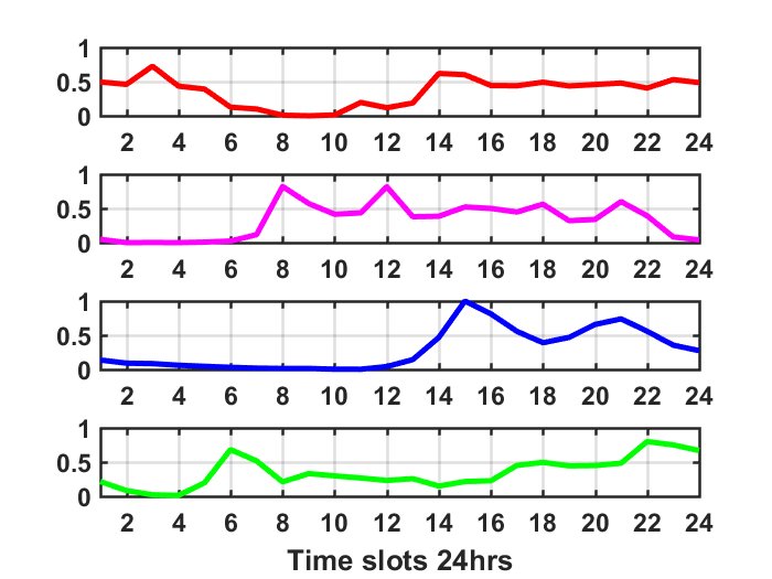
For LBSN datasets such as Gowalla, we have time as the mode. By setting the rank of a tensor as in the factorization process, we identified different patterns in the temporal factor matrix. Table 4 shows the PD values of all algorithms on the Gowalla dataset. SaCD outperforms all the baselines. GCD ran out of time due to the large mode length of the tensor. While FMU and FHALS can execute due to the low rank setting, they are not able to distinguish the patterns distinctly.
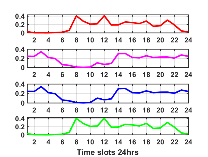
In Figure 7, we plot the values of the factor matrix in “temporal mode”, which have as and represents the normalized value of the factor matrix in each column. Figure 7(e) shows the patterns obtained by SaCD. The red pattern shows a peak at and that probably indicates the lunch and dinner time. The pink pattern shows a very common to activity. On the other hand, the blue pattern shows a unique pattern with a peak at , indicating night time activity. The green pattern shows activities between and . With a proper domain knowledge, the kind of activities that happens in different time periods can be easily interpreted by using distinct patterns. It is interesting to note that unlike FMU and CDTF, SaCD avoids simultaneous elimination problem (a state where similar patterns are derived multiple times) (Zou and Yuan 2008). In Figure 7(a), pink and blue patterns are highly similar, and in Figure 7(d), red pattern is same as the green pattern and pink pattern is same as the blue pattern. In comparison, patterns derived from SaCD are highly distinctive.
| Algorithm | PD | Runtime in secs |
|---|---|---|
| FMU | ||
| FHALS | ||
| BCDP | ||
| CDTF | ||
| GCD | ||
| SaCD | 0.34 | 363.27 |



6.8. Parallelization
Figure 3(d) shows the time taken for and the factor matrix update without multi-core parallelization. SaCD allows to minimize the time taken for factor matrix update by avoiding the frequent gradient calculation, however, the complexity of remains the same as the traditional element selection-based CD algorithm.
If the calculation of is parallelized as in the proposed algorithm FSaCD and executed using the cores of a single machine, the time taken for can be reduced as shown in Figure 8(a). We evaluate FSaCD in terms of mode length, density, and rank of the tensor. We set the rank to and density to to evaluate the performance in terms of mode length. As shown in Figure 8(b), FSaCD shows up to times fast computing comparing to GCD, the next best algorithm. By setting the rank to and mode length to , we decreased the density to evaluate the performance in terms of density. As shown in Figure 8(c), FSaCD shows up to fast computing performance in comparision to GCD. It is interesting to note that SaCD and FSaCD show similar performance on sparse datasets showing that parallelization has no effect. To evaluate the performance in terms of rank, we set the density to and the mode length of the tensor to and increased the rank from to . FSaCD shows improved performance in comparision to CDTF as shown in Figure 8(d). It ascertains that FSaCD can handle higher rank easily. It is also interesting to note that FSaCD shows a converged performance for ranks where the increase in the rank does not increase the runtime.
7. Conclusion
In this paper, we propose an element selection-based coordinate descent algorithm SaCD that measures the important elements for optimization using Lipschitz continuity and provides the saturated point for early stopping. The proposed Lipschitz continuity based element importance calculation introduces an additional regularity condition to the optimization process and helps to speed-up the convergence. SaCD can efficiently process NTF with higher mode length, rank, and density by reducing the frequent gradient updates. We also extend SaCD (called FSaCD) for the parallel environment to further improve the performance. We conducted theoretical and empirical studies to demonstrate the efficiency of SaCD. Theoretical analysis shows the time complexity and memory requirement as well as proves the fast convergence property of SaCD. Empirical analysis shows the superiority of SaCD and FSaCD in comparison to the state-of-the-art algorithms, in terms of tensor size (mode length), rank, and density without compromising the accuracy. Results show the applicability of SaCD in recommendation and pattern mining where efficiency is achieved at no cost of accuracy. SaCD and FSaCD require the element importance matrix stored in the memory which makes it challenging to extend in a distributed environment. In future work, we will explore SaCD and FSaCD to effectively handle the datasets in the distributed environment.
Acknowledgement
We like to express our gratitude to Dr. U Kang, Associate Professor, Seoul National University for his comments that had greatly improved the manuscript. His willingness to give his time so generously is very much appreciated.
References
- (1)
- Acar et al. (2011) Evrim Acar, Tamara G Kolda, and Daniel M Dunlavy. 2011. All-at-once optimization for coupled matrix and tensor factorizations. arXiv preprint arXiv:1105.3422 (2011).
- Adomavicius and Tuzhilin (2005) Gediminas Adomavicius and Alexander Tuzhilin. 2005. Toward the next generation of recommender systems: A survey of the state-of-the-art and possible extensions. IEEE Transactions on Knowledge & Data Engineering 6 (2005), 734–749.
- Bader and Kolda (2007) Brett W Bader and Tamara G Kolda. 2007. Efficient MATLAB computations with sparse and factored tensors. SIAM Journal on Scientific Computing 30, 1 (2007), 205–231.
- Bader et al. (2017) Brett W. Bader, Tamara G. Kolda, et al. 2017. MATLAB Tensor Toolbox Version 3.0-dev. Available online. https://www.tensortoolbox.org
- Balasubramaniam et al. (2018a) Thirunavukarasu Balasubramaniam, Richi Nayak, and Chau Yuen. 2018a. Nonnegative coupled matrix tensor factorization for smart city spatiotemporal pattern mining. In Machine Learning, Optimization and Data Science (LOD), The Fourth International Conference on. Springer.
- Balasubramaniam et al. (2018b) Thirunavukarasu Balasubramaniam, Richi Nayak, and Chau Yuen. 2018b. People to people recommendation using coupled nonnegative Boolean matrix factorization. In Soft-Computing and Network Security (ICSNS), 2018 International Conference on. IEEE.
- Balasubramaniam et al. (2019) Thirunavukarasu Balasubramaniam, Richi Nayak, and Chau Yuen. 2019. Sparsity constraint Nonnegative Tensor Factorization for mobility pattern mining. In Pacific Rim International Conference on Artificial Intelligence. Springer, 582–594.
- Beutel et al. (2014) Alex Beutel, Partha Pratim Talukdar, Abhimanu Kumar, Christos Faloutsos, Evangelos E Papalexakis, and Eric P Xing. 2014. Flexifact: Scalable flexible factorization of coupled tensors on hadoop. In Proceedings of the 2014 SIAM International Conference on Data Mining. SIAM, 109–117.
- Bouadjenek et al. (2016) Mohamed Reda Bouadjenek, Hakim Hacid, and Mokrane Bouzeghoub. 2016. Social networks and information retrieval, how are they converging? A survey, a taxonomy and an analysis of social information retrieval approaches and platforms. Information Systems 56 (2016), 1–18.
- Carroll and Chang (1970) J Douglas Carroll and Jih-Jie Chang. 1970. Analysis of individual differences in multidimensional scaling via an N-way generalization of “Eckart-Young” decomposition. Psychometrika 35, 3 (1970), 283–319.
- Choi and Vishwanathan (2014) Joon Hee Choi and S Vishwanathan. 2014. DFacTo: Distributed factorization of tensors. In Advances in Neural Information Processing Systems. 1296–1304.
- Cichocki et al. (2009) Andrzej Cichocki, Rafal Zdunek, Anh Huy Phan, and Shun-ichi Amari. 2009. Nonnegative matrix and tensor factorizations: applications to exploratory multi-way data analysis and blind source separation. John Wiley & Sons.
- Dunlavy et al. (2011) Daniel M Dunlavy, Tamara G Kolda, and Evrim Acar. 2011. Temporal link prediction using matrix and tensor factorizations. ACM Transactions on Knowledge Discovery from Data (TKDD) 5, 2 (2011), 10.
- Ermiş et al. (2015) Beyza Ermiş, Evrim Acar, and A Taylan Cemgil. 2015. Link prediction in heterogeneous data via generalized coupled tensor factorization. Data Mining and Knowledge Discovery 29, 1 (2015), 203–236.
- Guan et al. (2012) Naiyang Guan, Dacheng Tao, Zhigang Luo, and Bo Yuan. 2012. NeNMF: An optimal gradient method for nonnegative matrix factorization. IEEE Transactions on Signal Processing 60, 6 (2012), 2882–2898.
- Hager (1979) William W Hager. 1979. Lipschitz continuity for constrained processes. SIAM Journal on Control and Optimization 17, 3 (1979), 321–338.
- Hsieh and Dhillon (2011) Cho-Jui Hsieh and Inderjit S Dhillon. 2011. Fast coordinate descent methods with variable selection for non-negative matrix factorization. In Proceedings of the 17th ACM SIGKDD international conference on Knowledge discovery and data mining. ACM, 1064–1072.
- Ifada and Nayak (2014) Noor Ifada and Richi Nayak. 2014. Tensor-based item recommendation using probabilistic ranking in social tagging systems. In Proceedings of the 23rd International Conference on World Wide Web. ACM, 805–810.
- Ifada and Nayak (2016) Noor Ifada and Richi Nayak. 2016. How relevant is the irrelevant data: leveraging the tagging data for a learning-to-rank model. In Proceedings of the ninth ACM international conference on web search and data mining. ACM, 23–32.
- Jaggi (2011) Martin Jaggi. 2011. Sparse convex optimization methods for machine learning. Ph.D. Dissertation. ETH Zurich.
- Kang et al. (2012) U Kang, Evangelos Papalexakis, Abhay Harpale, and Christos Faloutsos. 2012. Gigatensor: scaling tensor analysis up by 100 times-algorithms and discoveries. In Proceedings of the 18th ACM SIGKDD international conference on Knowledge discovery and data mining. ACM, 316–324.
- Karatzoglou et al. (2010) Alexandros Karatzoglou, Xavier Amatriain, Linas Baltrunas, and Nuria Oliver. 2010. Multiverse recommendation: n-dimensional tensor factorization for context-aware collaborative filtering. In Proceedings of the fourth ACM conference on Recommender systems. ACM, 79–86.
- Khamaru and Wainwright (2018) Koulik Khamaru and Martin Wainwright. 2018. Convergence guarantees for a class of non-convex and non-smooth optimization problems. In International Conference on Machine Learning. 2606–2615.
- Kimura and Kudo (2015) Keigo Kimura and Mineichi Kudo. 2015. Variable Selection for Efficient Nonnegative Tensor Factorization. In Data Mining (ICDM), 2015 IEEE International Conference on. IEEE, 805–810.
- Kolda and Bader (2009) Tamara G Kolda and Brett W Bader. 2009. Tensor decompositions and applications. SIAM review 51, 3 (2009), 455–500.
- Kutty et al. (2012) Sangeetha Kutty, Lin Chen, and Richi Nayak. 2012. A people-to-people recommendation system using tensor space models. In Proceedings of the 27th Annual ACM Symposium on Applied Computing. ACM, 187–192.
- Lathauwer (2008) L De Lathauwer. 2008. Decompositions of a higher-order tensor in block terms—Part I: Lemmas for partitioned matrices. SIAM J. Matrix Anal. Appl 30, 3 (2008), 1022–1032.
- Lee and Seung (2001) Daniel D Lee and H Sebastian Seung. 2001. Algorithms for non-negative matrix factorization. In NIPS. 556–562.
- Liu and Xiong (2013) Bin Liu and Hui Xiong. 2013. Point-of-interest recommendation in location based social networks with topic and location awareness. In Proceedings of the 2013 SIAM International Conference on Data Mining. SIAM, 396–404.
- Nesterov (2012) Yu Nesterov. 2012. Efficiency of coordinate descent methods on huge-scale optimization problems. SIAM Journal on Optimization 22, 2 (2012), 341–362.
- Nguyen and Ho (2016) Duy Khuong Nguyen and Tu Bao Ho. 2016. Fast parallel randomized algorithm for nonnegative matrix factorization with KL divergence for large sparse datasets. arXiv preprint arXiv:1604.04026 (2016).
- Oh et al. (2017) Jinoh Oh, Kijung Shin, Evangelos E Papalexakis, Christos Faloutsos, and Hwanjo Yu. 2017. S-hot: Scalable high-order tucker decomposition. In Proceedings of the Tenth ACM International Conference on Web Search and Data Mining. ACM, 761–770.
- Park et al. (2016) Namyong Park, Byungsoo Jeon, Jungwoo Lee, and U Kang. 2016. Bigtensor: Mining billion-scale tensor made easy. In Proceedings of the 25th ACM International on Conference on Information and Knowledge Management. ACM, 2457–2460.
- Phan et al. (2012) Anh Huy Phan, Petr Tichavskỳ, and Andrzej Cichocki. 2012. On fast computation of gradients for CANDECOMP/PARAFAC algorithms. arXiv preprint arXiv:1204.1586 (2012).
- Phan et al. (2013) Anh-Huy Phan, Petr Tichavskỳ, and Andrzej Cichocki. 2013. Fast alternating LS algorithms for high order CANDECOMP/PARAFAC tensor factorizations. IEEE Transactions on Signal Processing 61, 19 (2013), 4834–4846.
- Rendle and Schmidt-Thieme (2010) Steffen Rendle and Lars Schmidt-Thieme. 2010. Pairwise interaction tensor factorization for personalized tag recommendation. In Proceedings of the third ACM international conference on Web search and data mining. ACM, 81–90.
- Sapienza et al. (2018) Anna Sapienza, Alessandro Bessi, and Emilio Ferrara. 2018. Non-negative tensor factorization for human behavioral pattern mining in online games. Information 9, 3 (2018), 66.
- Shin and Kang (2014) Kijung Shin and U Kang. 2014. Distributed methods for high-dimensional and large-scale tensor factorization. In ICDM. IEEE, 989–994.
- Shin et al. (2017) Kijung Shin, Lee Sael, and U Kang. 2017. Fully scalable methods for distributed tensor factorization. IEEE Transactions on Knowledge and Data Engineering 29, 1 (2017), 100–113.
- Sidiropoulos et al. (2017) Nicholas D Sidiropoulos, Lieven De Lathauwer, Xiao Fu, Kejun Huang, Evangelos E Papalexakis, and Christos Faloutsos. 2017. Tensor decomposition for signal processing and machine learning. IEEE Transactions on Signal Processing 65, 13 (2017), 3551–3582.
- Smith et al. (2015) Shaden Smith, Niranjay Ravindran, Nicholas D Sidiropoulos, and George Karypis. 2015. SPLATT: Efficient and parallel sparse tensor-matrix multiplication. In Parallel and Distributed Processing Symposium (IPDPS), 2015 IEEE International. IEEE, 61–70.
- Sra et al. (2008) Suvrit Sra, Dongmin Kim, and Bernhard Schölkopf. 2008. Non-monotonic poisson likelihood maximization. Max Planck Institute for Biological Cybernetics, Tech. Rep 170 (2008).
- Sun and Axhausen (2016) Lijun Sun and Kay W Axhausen. 2016. Understanding urban mobility patterns with a probabilistic tensor factorization framework. Transportation Research Part B: Methodological 91 (2016), 511–524.
- Symeonidis (2016) Panagiotis Symeonidis. 2016. Matrix and tensor factorization with recommender system applications. Graph-Based Social Media Analysis 39 (2016), 187.
- Symeonidis et al. (2013) Panagiotis Symeonidis, Antonis Krinis, and Yannis Manolopoulos. 2013. Geosocialrec: Explaining recommendations in location-based social networks. In East European Conference on Advances in Databases and Information Systems. Springer, 84–97.
- Symeonidis et al. (2008) Panagiotis Symeonidis, Alexandros Nanopoulos, and Yannis Manolopoulos. 2008. Tag recommendations based on tensor dimensionality reduction. In Proceedings of the 2008 ACM conference on Recommender systems. ACM, 43–50.
- Symeonidis et al. (2009) Panagiotis Symeonidis, Alexandros Nanopoulos, and Yannis Manolopoulos. 2009. A unified framework for providing recommendations in social tagging systems based on ternary semantic analysis. IEEE Transactions on Knowledge and Data Engineering 22, 2 (2009), 179–192.
- Takane et al. (1977) Yoshio Takane, Forrest W Young, and Jan De Leeuw. 1977. Nonmetric individual differences multidimensional scaling: An alternating least squares method with optimal scaling features. Psychometrika 42, 1 (1977), 7–67.
- Tucker (1966) Ledyard R Tucker. 1966. Some mathematical notes on three-mode factor analysis. Psychometrika 31, 3 (1966), 279–311.
- Wright (2015) Stephen J Wright. 2015. Coordinate descent algorithms. Mathematical Programming 151, 1 (2015), 3–34.
- Xu and Yin (2013) Yangyang Xu and Wotao Yin. 2013. A block coordinate descent method for regularized multiconvex optimization with applications to nonnegative tensor factorization and completion. SIAM Journal on imaging sciences 6, 3 (2013), 1758–1789.
- Yu et al. (2012) Hsiang-Fu Yu, Cho-Jui Hsieh, Si Si, and Inderjit Dhillon. 2012. Scalable coordinate descent approaches to parallel matrix factorization for recommender systems. In ICDM. IEEE, 765–774.
- Yu and Chen (2015) Yonghong Yu and Xingguo Chen. 2015. A survey of point-of-interest recommendation in location-based social networks. In Workshops at the Twenty-Ninth AAAI Conference on Artificial Intelligence, Vol. 130.
- Zhang et al. (2016) Yu Zhang, Guoxu Zhou, Qibin Zhao, Andrzej Cichocki, and Xingyu Wang. 2016. Fast nonnegative tensor factorization based on accelerated proximal gradient and low-rank approximation. Neurocomputing 198 (2016), 148–154.
- Zheng et al. (2010) Nan Zheng, Qiudan Li, Shengcai Liao, and Leiming Zhang. 2010. Which photo groups should I choose? A comparative study of recommendation algorithms in Flickr. Journal of Information Science 36, 6 (2010), 733–750.
- Zheng et al. (2014) Yu Zheng, Tong Liu, Yilun Wang, Yanmin Zhu, Yanchi Liu, and Eric Chang. 2014. Diagnosing New York city’s noises with ubiquitous data. In Proceedings of the 2014 ACM International Joint Conference on Pervasive and Ubiquitous Computing. ACM, 715–725.
- Zou and Yuan (2008) Hui Zou and Ming Yuan. 2008. The F-norm support vector machine. Statistica Sinica (2008), 379–398.