Reduced Order Modeling of Diffusively Coupled Network Systems:
An Optimal Edge Weighting Approach
Abstract
This paper studies reduced-order modeling of dynamic networks with strongly connected topology. Given a graph clustering of an original complex network, we construct a quotient graph with less number of vertices, where the edge weights are parameters to be determined. The model of the reduced network is thereby obtained with parameterized system matrices, and then an edge weighting procedure is devised, aiming to select an optimal set of edge weights that minimizes the approximation error between the original and the reduced-order network models in terms of -norm. The effectiveness of the proposed method is illustrated by a numerical example.
I Introduction
With the growing complexity of spatially interconnected dynamic systems, the importance of understanding and managing dynamic networks has been widely recognized. An important class of dynamic networks is given by the so-called diffusively coupled networks, which are commonly used for describing diffusion processes, e.g., information or energy spreading in networks. The examples can be found in vehicle formations, electrical networks, synchronization in sensor networks, and opinion dynamics in social networks, see e.g. [1, 2, 3, 4]. The spatial structures of such systems are usually complex and result in high-dimensional models that cause challenges for analysis, control, and optimization. To effectively capture the collective behaviors of dynamics over networks, it is desirable to simplify the structure of a complex network without a significant loss of accuracy.
Different from model reduction problems for other types of dynamic systems, the one considered in this paper puts emphasis on the preservation of the network structure, which is necessary for applications e.g., distributed controller design and sensor allocation [5, 6, 7]. Conventional model reduction methods, e.g., balanced truncation and moment matching, merely focus on approximating the input-output behavior of a given dynamic system [8], while the preservation of the network structure is barely guaranteed. Although a generalized balanced truncation approach in [9] is able to construct an accurate reduced-order model with a network interpretation, the relation between the original and obtained new typologies is not yet clear. Singular perturbation approximation, as alternative network structure-preserving approach, has been applied to the reduction of electric circuits [10] and chemical reaction networks [11]. This class of methods mainly relies on time-scale separation of the states in an autonomous network system, while the external inputs are not considered explicitly. Besides, the resulting reduced topology hardly retains sparsity.
Recently, clustering-based methods have been intensively studied and become the mainstream methodology for reducing network systems, see e.g., [12, 13, 14, 15, 16, 17, 18, 19, 20]. With graph clustering, the vertices in a large-scale network are partitioned into several disjoint clusters. This class of methods has a clear advantage in retaining the consensus property [12, 19], system positivity [15], and scale-free property [20] in reduced-order models. The model reduction procedure can be implemented via the Petrov-Galerkin projection framework, where the projection matrix is formed based on the vertex clusters. However, all the current clustering-based methods put their main focus on finding suitable clusters. After clusters are found, reduced-order network models are then directly determined by the projection framework, while the freedom to construct a reduced-order network model with higher accuracy is overlooked.
In this paper, we will explore the latter freedom and provide a novel method for reduced-order modeling of directed networks. We do not aim to find an optimal clustering. Instead, we assume that the clustering of a network is given, which leads to a quotient graph. A parameterized reduced-order model is established based on this quotient graph, in which the edge weights are free variables to be optimized. Then, the major problem in this paper follows: How to tune the edge weights in the parameterized reduced-order model to minimize the approximation error?
This problem can be formulated as an optimization problem with the objective to minimize the -norm of the reduction error between original and reduced network systems, in which the edge weights of the reduced network are variables to be optimized. This edge weighting problem is subject to a bilinear matrix inequality (BMI) constraint, which is computationally expensive. Therefore, we devise a novel edge weighting algorithm based on the convex-concave decomposition, which linearizes the nonconvex constraint as a convex one in the form of a linear matrix inequality (LMI). An iterative scheme is implemented to search for a set of optimal weights. The convergence of this algorithm is theoretically ensured, and thus at least a local optimum can be reached. Moreover, we initialize the edge weights as the outcome of clustering-based projection, such that the obtained reduced-order network model is guaranteed a better approximation accuracy than the clustering-based projection methods.
The rest of this paper is organized as follows. In Section II, we recap some preliminaries on graph theory and introduce the problem setup. In Section III, the parameterized reduced-order model is formulated, and an edge weighting algorithm is proposed to minimize the approximation error. In Section IV, the proposed method is illustrated by an example, and Section V finally makes some concluding remarks.
Notation: The symbol and denote the set of real numbers and positive real numbers, respectively. Let be the set of real symmetric matrices of size . is the identity matrix of size , and represents the vector in of all ones. The cardinality of a set is denoted by . For a real matrix , the columns of form a basis of the null space of , that is, .
II Preliminaries and Problem Setting
This section provides necessary definitions and concepts in graph theory used in this paper, and we refer to [21] for more details. The model of a dynamical network is then introduced and the model reduction problem is formulated.
II-A Graph Theory
A directed graph consists of a finite and nonempty node set and an edge set . Each element in is an ordered pair of , and if , we say that the edge is directed from vertex to vertex . A directed graph is called simple, if does not contain self-loops (i.e., does not contain any edge of the form , ), and there exists only one edge directed from to , if .
Next, we introduce several important matrices for characterizing a directed simple graph. Let , the incidence matrix is defined by
If each edge is assigned a positive value (weight), then the weighted adjacency matrix of , denoted by , is defined such that denotes the weight of edge , and if . In the case of a simple graph, is a binary matrix with zeros on its diagonal. Then, the Laplacian matrix of the graph is defined as
| (1) |
Clearly, . The diagonal entries of are strictly positive, and the off-diagonal entries are non-positive. Alternatively, we can characterize the Laplacian matrix using the incidence matrix of as
| (2) |
where is a binary matrix obtained by replacing all “” entries in the incidence matrix with zeros, and
and the positive weight associated to the -th edge, for all .
For a vertex in a weighted graph, the indegree and outdegree of the vertex are computed as and , respectively. A strongly connected graph is called balanced if the indegree and outdegree of each vertex in is equal. From (1), the following lemma is immediate.
Lemma 1.
A weighted strongly connected graph is balanced if and only if one of the following conditions hold.
- 1.
The edge weights of satisfies
- 2.
The Laplacian matrix of satisfies
The strong connectivity implies that there is only one zero eigenvalue of [21], and the balance of then indicates that both the row and column sums of are zero.
Remark 1.
Undirected graphs can be viewed as special balanced directed graphs with bidirectional edges. The Laplacian matrix of an undirected graph is where is an incidence matrix obtained by assigning an arbitrary orientation to each edge of the undirected graph, and is a positive diagonal matrix representing edge weights.
Next, we recapitulate the notion of graph clustering, whose concept can be found in e.g., [12, 15, 14, 13, 16, 17].
Definition 1.
Let be a directed graph. Then, a graph clustering is a partition of into nonempty disjoint subsets covering all the elements in , where is called a cluster of .
Let be a clustering of with vertices. This graph clustering can be characterized by a binary characteristic matrix , whose rows and columns are corresponding to the vertices and clusters, respectively:
Remark 2.
Note that all the clusters are nonoverlapping, i.e., each vertex can be not assigned to distinct clusters. Therefore, each row of the characteristic matrix only has one nonzero element. Specifically, we have
| (3) |
II-B Problem Setup
In this paper, we consider a network system evolving over a directed graph , which is simple, weighted and strongly connected. The dynamics of each vertex is governed by
| (4) |
where is the state of vertex , and is the -th entry of the adjacency matrix of , representing the strength of the coupling between vertices and . is the external input, and is the gain of the -th input acting on vertex , which is zero if and only if has no effect on vertex . Let be the matrix such that . We then present the dynamics of the overall network in a compact form as
| (5) |
with and . The vector collects the outputs of the network, and is the output matrix.
This paper aims for structure-preserving model reduction of diffusively coupled networks in form of (5), and the reduced-order model not only approximates the input-output mapping of the original network system with a certain accuracy but also inherits an interconnection structure with diffusive couplings. To this end, we adopt graph clustering to build up a reduced-order network model. Specifically, the problem addressed in this paper is as follows.
Problem 1.
Given a network system as in (5) and a graph clustering , find a reduced-order model
| (6) |
with , , such that is the Laplacian matrix of a reduced directed graph, and the reduction error is minimized. , , are matrices depending on the graph clustering.
It is worth emphasizing that Problem 1 does not aim to find an appropriate graph clustering of the network . Instead, we focus on how to establish a “good” reduced-order model with given clusters. Thus, it is an essentially different problem from e.g., [17, 19, 14, 15], and we do not apply the Petrov-Galerkin projection framework.
III Main Result
In this section, a novel model reduction approach for network systems is presented with two steps. In the fist step, a parameterized model of a reduced network is constructed on the basis of graph clustering. Then, the second step computes a set of parameters in an optimal fashion such that the -norm of approximation error is minimized.
III-A Parameterized Reduced-Order Network Model
Given a graph clustering of the original network, we present a parameterized model for the reduced network, whose interconnection topology is determined by the clustering. An important property of this parameterized model is that it guarantees the boundedness of the reduction error for all positive edge weights.
To derive a parameterized reduced-order network model with such a property, we first convert the system (5) to its balanced graph representation as follows.
Lemma 2.
If the underlying graph of in (5) is strongly connected, then there exists a diagonal with positive diagonal entries such that is equivalent to
| (7) |
where and is the Laplacian of a balanced graph.
The proof follows directly from [19]. Next, we establish a reduced-order model using the representation (7) to guarantee a bounded reduction error .
Let be the balanced graph of . Note that and have the same incidence matrix . Given a graph clustering , the quotient graph is -vertex directed graph obtained by aggregating all the vertices in each cluster as a single vertex, while retaining connections between clusters and ignoring the edges within clusters. Specifically, if there is an edge in with vertices in the same cluster, then it will not be presented as an edge in . If there exists an edge with and , then there is an edge in .
Let be the incidence matrix of the quotient graph . Algebraically, it can be verified that is obtained by removing all the zero columns of , where is the incidence matrix of (or ). Furthermore, we denote
| (8) |
as the edge weight matrix of , where , and is number of edges in . In order to maintain as a balanced graph, we impose the constraint on its edge weights as
| (9) |
according to Lemma 3. Thereby, the dynamics on the balanced quotient graph is then obtained as
| (10) |
with the reduced matrices
| (11) |
where is the binary matrix obtained by replacing all the “” entries with zeros in , and , , and are reduced matrices determined by the given clustering of . Since the graph clustering is given, i.e., is known, the only parameters to be decided are the weights in , which satisfy the constraint (9).
From the reduced graph balanced representation (10), we immediately construct a parameterized reduced-order model in the form of (6) with the reduced matrices
| (12) |
where represents a reduced weighted graph . In (12), only the weight matrix is to be determined, which is selected from the following set
| (13) |
In the following example, we demonstrate the parameterized modeling of a simplified dynamic network.
Example 1.
Consider an network example in vehicle formation [1], where the formation topology is depicted in Fig. 1. Clearly, is balanced, i.e., , with the incidence matrix
Suppose that each vehicle is modeled as a first-order integrator which has the identical mass, i.e., . An external control is applied on vertex 4, and the vertex 1 is measured as the output signal . Then, the network model is obtained in the form of (7) with
Consider a clustering of as , which leads to the characterization matrix as
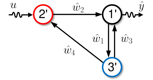
The topology of the quotient graph is shown in Fig. 1 with the incidence matrix
All the edge weights of are positive parameters to be determined, as labeled in Fig. 1, which leads to the parameterized Laplacian matrix as
The weights satisfy the constraint , namely, , , such that is balanced. The other matrices in the reduced-order model (10) are computed as
Then, in the parameterized reduced-order model 6, we have
with , and . The corresponding reduced graph is depicted in Fig. 1, which is no longer balanced.


Remark 3.
The physical interpretation of the reduced matrices in (III-A) are explained. is constructed such that the mass of vertex in is equal to the mass sum of all the vertices in in . The expression of means that if a vertex in a cluster of is controlled by an external input, then vertex in is also controlled. Analogously, indicates that a vertex in is measured if there is a measurement taken from a vertex in .
With the reduced matrices in (12) and the constraint in (9), an important property of the reduced-order network model is that it guarantees the reduction error between the original system in (5) and is always bounded.
The computation of the reduction error amounts to find the norm of the following error system:
| (14) |
where
Note that is not Hurwitz, since and are both Laplacian matrices containing zero eigenvalues. Thus, cannot be calculated directly using the state space representation (14). Here, we employ the following matrices
| (15) |
which are independent of system dynamics and satisfy
Let their left pseudo inverses be
Then, using the matrices in (15), we show the following result.
Lemma 3.
Proof.
With and in (15), we construct a nonsingular matrix as
| (16) |
where . The inverse of is given as
Note that and , where both and are the Laplacian matrices of balanced graphs, satisfying , , and , . Using these properties, we obtain
| (17) |
where
| (18) |
and
| (19) |
It follows from (3) that , and , which yield Thus, (III-A) becomes
| (20) |
It is not hard to verify that both the matrices and are Hurwitz. Consequently, in (20) is asymptotically stable, i.e., , for all . ∎
Next, we discuss the consensus property of the reduced-order network (6) with the matrices in (12). Consensus is a typical property of diffusively coupled networks, and it implies the nodal states converge to a common value in the absence of the external input. More precisely, the network system in (5) reaches consensus if
holds for all and all initial conditions.
Proposition 1.
Proof.
The parameterized modeling of the reduced dynamic network using the graph balanced representation in (7) guarantees the stability of the error system (14), whose norm can be evaluated via the transfer function (20) with the Hurwitz matrix . Note that in (20), the matrices and in (15) is only dependent on the sizes of the networks, and is known for a given graph clustering, then the weights in become the only unknown parameters to be determined in the follow-up procedure. In the following section, we aim for an optimal selection of the edges weights in the reduced network.
III-B Optimal Edge Weighting
In this section, we aim for an optimization scheme for determining that minimizes the approximation error . Thereby, the following problem is addressed.
Problem 2.
To solve this problem, we apply an optimization technique based on the convex-concave decomposition, which can be implemented to search for a set of optimal weights iteratively. A fundamental step toward the implementation is to develop a necessary and sufficient condition for characterizing , which leads to suitable constraints for the optimization problem.
Theorem 1.
Proof.
Consider the error system in (20), which is asymptotically stable. Following e.g., [22], we have , with , if and only if there exist matrices and such that
| (25) | |||||
| (26) | |||||
| (27) |
where , , are defined in (III-A).
In the following, we prove that the three inequalities are equivalent to (21), (22), and (23), respectively. First, it is not hard to verify that (25) is equivalent to
| (28) |
for a sufficiently large scalar , where is defined in (1). Consider a nonsingular matrix
Pre- and post-multiplying by and , respectively, (28) then becomes (21), where the equation , and the substitutions , are used.
Based on Theorem 1, we reformulate Problem 2 more explicitly as the following minimization problem
| (29) | ||||
where with a given . Note that the constraint (22) can be solved efficiently using standard LMI solvers, while (21), due to the nonlinearity term , is a bilinear matrix inequality, which causes the major challenge in solving the problem (29).
To handle the bilinear constraint (21), we adopt the technique called psd-convex-concave decomposition [23].
Definition 2.
A matrix-valued mapping is called positive semidefinite convex concave (psd-convex-concave) if can be expressed as , where , with , are positive semidefinite convex (psd-convex), i.e.,
| (30) |
holds for all and . The pair is called a psd-convex-concave decomposition of .
Consider the bilinear inequality (21), and define the following matrix-valued mapping:
| (31) |
where
| (32) | ||||
| (33) |
Then, the following lemma shows that the pair is a psd-convex-concave decomposition of .
Lemma 4.
The matrix-valued mapping in (31) is psd-convex-concave.
Proof.
Note that the matrix in (31) is linear with respect to and . Thus, it is immediate that is psd-convex. Then, the claim holds if in (31) is psd-convex.
The psd-convex-concave decomposition in (31) allows us to linearize the optimization problem (29) at a stationary point . To simplify the optimization procedure, we introduce a new optimization variable to eliminate the equality constraint in (13), where , and is the number of edges in the reduced network.
Let be a full row rank matrix obtained by removing linearly independent rows of the , and it still holds that . Then, there exists a column permutation matrix such that
where is full rank. , and , is defined as the new optimization variable. Note that
| (36) |
which projects the weights into . Thereby, we rewrite the constraint as (36). Now, we redefine the matrix-valued mapping in (31) as
| (37) |
which remains psd-convex due to the linear relation in (36). The derivative of the matrix-valued mapping at is a linear mapping , with , which is defined as
| (38) |
Given a point , the linearized formulation of the problem (29) at is formulated as
| (39) | ||||
where the derivative of is given as
with Notice that the optimization problem (39) is convex, of which the global optimum can be solved efficiently using standard SDP solvers e.g., SeDuMi [24]. Based on Lemma 4 and (39), we are now ready to present an algorithmic approach for solving the minimization problem in (29) in an iterative fashion, see Algorithm 1, in which is a prefixed error tolerance determining whether to terminate the iteration loop.
The initial condition can be chosen as an arbitrary vector with all strictly positive entries. With (36), it will guarantee , i.e., the reduced graph is balanced. Furthermore, we can also initialize using the outcome of graph clustering projection in [18, 19]. Specifically, from a given clustering , we construct an initial reduced Laplacian matrix in (III-A) as , with the Laplacian matrix of the balanced graph . Then, the initial weight of the edge in the quotient graph is the -th entry of . By doing so, can be formed such that .
The convergence analysis of Algorithm 1 follows naturally from [23], and it means that a local optimum can be obtained. More importantly, if we select the initial condition from the clustering-based projection, it is guaranteed that, through iteration, the approximation accuracy of reduced-order network model with the weights obtained by Algorithm 1 will be improved. In this sense, the approximations obtained by the proposed method is at least better than the ones obtained by clustering-based projection methods in e.g., [18, 19]. We will show this merit from a numerical example in the next section.
IV Illustrative Example
To illustrate the effectiveness of the proposed edge weighting approach, we implement it to a sensor network example from [3, 18]. The topology of the this network is shown in Fig. 2, which consists of 14 strongly connected vertices, and all the edge weights are 1. In this example, two external input signals are injected into the network via vertices 2 and 7, respectively, and the states of vertices 9 and 10 are measured.
Suppose that 5 clusters are given for this directed network as which leads to the quotient network in Fig. 3, with incidence matrix
There are 8 edges in the quotient graph, and each edge is assigned with a symbolic weight as labeled in Fig. 3. These variables, determining the reduction error, are to be determined by our optimization approach.
First, the parameterized reduced model in (10) of the quotient graph is generated with matrices
and the weight vector in (8) satisfy the following constraints for a balanced graph:
Next, we implement Algorithm 1 to solve the optimization problem (29) with as the optimization variable. Particularly, the SeDuMi solver [24] is adopted to solve the convex problem (39). We choose the initial edge weights obtained by the clustering-based projection [18, 19], which gives and the approximation error . With , Algorithm 1 stops after 72 iterations. The convergence trajectory of the resulting reduction error is shown in Fig. 4. The final solution of the edge weights are given as , which provides the approximation error . Through iteration, the edge weighting method further reduces the error by 41.93%, compared to the clustering-based projection. Therefore, our method can provide a reduced network systems with a better approximation error.


V Conclusions
In this paper, the model reduction problem for dynamical networks consisting of diffusively coupled agents has been formulated as a minimization problem, in which the edge weights in the reduced network are parameters to be chosen. Necessary and sufficient conditions have been proposed for constructing a set of optimal edge weights. An iterative algorithm has been provided to search for the desired edge weights such that the norm of the approximation error is small. Finally, compared with the projection-based method in [12], the feasibility of this method is illustrated by an example. The advantage of this proposed model reduction method is that not only the structure of the original network has been preserved but also the approximation error has been optimized. For future works, we will improve the effectiveness of the iterative algorithm such that the obtained solution is not restricted to a local optimum. Moreover, an extension to networked high-order linear subsystems are also of interest.
References
- [1] J. A. Fax and R. M. Murray, “Graph Laplacians and stabilization of vehicle formations,” 2001.
- [2] F. Dörfler, J. W. Simpson-Porco, and F. Bullo, “Electrical networks and algebraic graph theory: Models, properties, and applications,” Proceedings of the IEEE, vol. 106, no. 5, pp. 977–1005, 2018.
- [3] G. Scutari, S. Barbarossa, and L. Pescosolido, “Distributed decision through self-synchronizing sensor networks in the presence of propagation delays and asymmetric channels,” IEEE Transactions on Signal Processing, vol. 56, no. 4, pp. 1667–1684, 2008.
- [4] A. V. Proskurnikov, A. S. Matveev, and M. Cao, “Opinion dynamics in social networks with hostile camps: Consensus vs. polarization,” IEEE Transactions on Automatic Control, vol. 61, no. 6, pp. 1524–1536, 2015.
- [5] T. H. Summers and J. Lygeros, “Optimal sensor and actuator placement in complex dynamical networks,” IFAC Proceedings Volumes, vol. 47, no. 3, pp. 3784–3789, 2014.
- [6] A. J. Gates and L. M. Rocha, “Control of complex networks requires both structure and dynamics,” Scientific Reports, vol. 6, no. 1, pp. 1–11, 2016.
- [7] T. Ishizaki, A. Chakrabortty, and J.-I. Imura, “Graph-theoretic analysis of power systems,” Proceedings of the IEEE, vol. 106, no. 5, pp. 931–952, 2018.
- [8] A. C. Antoulas, Approximation of Large-Scale Dynamical Systems. Philadelphia, USA: SIAM, 2005.
- [9] X. Cheng, J. M. A. Scherpen, and B. Besselink, “Balanced truncation of networked linear passive systems,” Automatica, vol. 104, pp. 17–25, 2019.
- [10] E. Bıyık and M. Arcak, “Area aggregation and time-scale modeling for sparse nonlinear networks,” Systems & Control Letters, vol. 57, no. 2, pp. 142–149, 2008.
- [11] S. Rao, A. J. van der Schaft, and B. Jayawardhana, “A graph-theoretical approach for the analysis and model reduction of complex-balanced chemical reaction networks,” Journal of Mathematical Chemistry, vol. 51, no. 9, pp. 2401–2422, 2013.
- [12] N. Monshizadeh, H. L. Trentelman, and M. K. Camlibel, “Projection-based model reduction of multi-agent systems using graph partitions,” IEEE Transactions on Control of Network Systems, vol. 1, pp. 145–154, Jun. 2014.
- [13] B. Besselink, H. Sandberg, and K. H. Johansson, “Clustering-based model reduction of networked passive systems,” IEEE Transactions on Automatic Control, vol. 61, no. 10, pp. 2958–2973, Oct 2016.
- [14] T. Ishizaki, K. Kashima, J. I. Imura, and K. Aihara, “Model reduction and clusterization of large-scale bidirectional networks,” IEEE Transactions on Automatic Control, vol. 59, pp. 48–63, 2014.
- [15] T. Ishizaki, K. Kashima, A. Girard, J.-i. Imura, L. Chen, and K. Aihara, “Clustered model reduction of positive directed networks,” Automatica, vol. 59, pp. 238–247, 2015.
- [16] H.-J. Jongsma, P. Mlinarić, S. Grundel, P. Benner, and H. L. Trentelman, “Model reduction of linear multi-agent systems by clustering with and error bounds,” Mathematics of Control, Signals, and Systems, vol. 30, no. 1, p. 6, 2018.
- [17] X. Cheng, Y. Kawano, and J. M. A. Scherpen, “Model reduction of multi-agent systems using dissimilarity-based clustering,” IEEE Transactions on Automatic Control, vol. 64, no. 4, pp. 1663–1670, April 2019.
- [18] X. Cheng and J. M. A. Scherpen, “A new controllability Gramian for semistable systems and its application to approximation of directed networks,” in Proceedings of IEEE 56th Conference on Decision and Control, Melbourne, Australia, Dec 2017, pp. 3823–3828.
- [19] X. Cheng and J. M. A. Scherpen, “Clustering-based model reduction of laplacian dynamics with weakly connected topology,” IEEE Transactions on Automatic Control, 2019.
- [20] N. Martin, P. Frasca, and C. Canudas-de Wit, “Large-scale network reduction towards scale-free structure,” IEEE Transactions on Network Science and Engineering, vol. 6, no. 4, pp. 711–723, 2018.
- [21] M. Mesbahi and M. Egerstedt, Graph Theoretic Methods in Multiagent Networks. Princeton University Press, 2010.
- [22] G. Pipeleers, B. Demeulenaere, J. Swevers, and L. Vandenberghe, “Extended LMI characterizations for stability and performance of linear systems,” Systems & Control Letters, vol. 58, no. 7, pp. 510–518, 2009.
- [23] Q. T. Dinh, S. Gumussoy, W. Michiels, and M. Diehl, “Combining convex-concave decompositions and linearization approaches for solving BMIs, with application to static output feedback,” IEEE Transactions on Automatic Control, vol. 57, no. 6, pp. 1377–1390, 2011.
- [24] J. F. Sturm, “Using SeDuMi 1.02, a MATLAB toolbox for optimization over symmetric cones,” Optimization Methods and Software, vol. 11, no. 1-4, pp. 625–653, 1999.