Recursive Least Squares
with Variable-Direction Forgetting
Compensating for the loss of persistency

Ankit Goel Adam L. Bruce Dennis S. Bernstein Affiliation: POC: A. Goel (ankgoel@umich.edu)

The ability to estimate parameters depends on two things, namely, identifiability [1], which is ability to distinguish distinct parameters, and persistent excitation, which refers to the spectral content of the signals needed to ensure convergence of the parameter estimates to the true parameter values [2, 3, 4]. Roughly speaking, the level of persistency must be commensurate with the number of unknown parameters. For example, a harmonic input has two-dimensional persistency and thus can be used to identify two parameters, whereas white noise is sufficiently persistent for identifying an arbitrary number of parameters. Within the context of adaptive control, persistent excitation is needed to avoid bursting [5]; recent research has focused on relaxing these requirements [6, 7, 8].

Under persistent excitation, a key issue in practice is the rate of convergence, especially under changing conditions. For example, the parameters of a system may change abruptly, and the goal is to ensure fast convergence to the modified parameter values. In this case, it turns out that the rate of convergence depends on the ability to forget past parameters and incorporate new information. As discussed in “Summary,” the ability to accommodate new information depends on the ability to forget; the ability to forget is thus crucial to the ability to learn. This paradox is widely recognized, and effective forgetting is of intense interest in machine learning [9, 10, 11, 12].

In the first half of the present article, classical forgetting within the context of recursive least squares (RLS) is considered. In the classical RLS formulation [13, 14, 15, 16], a constant forgetting factor $\lambda\in(0,1]$ can be set by the user. However, it often occurs in practice that the performance of RLS is extremely sensitive to the choice of $\lambda$ , and suitable values in the range $0.99$ to $0.9999$ are typically found by trial-and-error testing. This difficulty has motivated extensions of classical RLS in the form of variable-rate forgetting [17, 18, 19, 20, 21, 22, 23], constant trace adjustment, covariance resetting, and covariance modification [24, 25].

In the second half of this article, variable-direction forgetting (VDF), a technique that complements variable-rate forgetting is considered. Direction-dependent forgetting has been widely studied within the context of recursive least squares [26, 27, 28, 29, 30, 31, 32]. In the absence of persistent excitation, new information is confined to a limited number of directions. The goal of VDF is thus to determine these directions and thereby constrain forgetting to the directions in which new information is available. VDF allows RLS to operate without divergence during periods of loss of persistency.

The goal of this tutorial article is to investigate the effect of forgetting within the context of RLS in order to motivate the need for VDF. With this motivation in mind, the article develops and illustrates RLS with VDF. The presentation is intended for graduate students who may wish to understand and apply this technique to system identification for modeling and adaptive control. Table 1 and 2 summarizes the results and examples in this article. Some of the content in this article appeared in preliminary form in [33].

Although, in practical applications, all sensor measurements are corrupted by noise, the effect of sensor noise is not considered in this article in order to focus on the loss of persistency. Alternative interpretations of RLS in the special case of zero-mean, white sensor noise are presented in “RLS as a One-Step Optimal Predictor” and “RLS as a Maximum Likelihood Estimator”.

TABLE 1: Summary of definitions and results in this article.

Definition 1	Persistently exciting regressor
Definition 2	Lyapunov stable equilibrium
Definition 3	Uniformly Lyapunov stable equilibrium
Definition 4	Globally aymptotically stable equilibrium
Definition 5	Uniformly globally geometrically stable equilibrium
Theorem 1-2	Recursive least squares (RLS)
Theorem 3-5	Lyapunov stability theorems
Theorem 6	Lyapunov analysis of RLS for $\lambda\in(0,1)$
Theorem 7	Stability analysis of RLS for $\lambda\in(0,1]$ based on $\theta_{k}$
Theorem S1	A Quadratic Cost Function for Variable-Direction RLS
Proposition 1	Recursive update of $P_{k}^{-1}$ with uniform-direction forgetting
Proposition 2	Data-dependent subspace constraint on $\theta_{k}$
Proposition 3	Bounds on $P_{k}$ for $\lambda=1$
Proposition 4	Bounds on $P_{k}$ for $\lambda\in(0,1)$
Proposition 5	Converse of Proposition 4
Proposition 6	Convergence of $z_{k}$ with uniform-direction forgetting
Proposition 7	Persistent excitation and ${\mathcal{A}}_{k}$
Proposition 8	Recursive update of $P_{k}^{-1}$ with variable-direction forgetting
Proposition 9	Convergence of $z_{k}$ with variable-direction forgetting
Proposition 10	Bounds on $P_{k}$ with variable-direction forgetting

TABLE 2: Summary of examples in this article.

Example 1	$P_{k}$ converges to zero without persistent excitation
Example 2	Persistent excitation and bounds on $P_{k}^{-1}$
Example 3	Lack of persistent excitation and bounds on $P_{k}^{-1}$
Example 4	Convergence of $z_{k}$ and $\theta_{k}$
Example 5	Using $\kappa(P_{k})$ to determine whether $(\phi_{k})_{k=0}^{\infty}$ is persistently exciting
Example 6	Effect of $\lambda$ on the rate of convergence of $\theta_{k}$
Example 7	Lack of persistent excitation in scalar estimation
Example 8	Subspace constrained regressor
Example 9	Effect of lack of persistent excitation on $\theta_{k}$
Example 10	Lack of persistent excitation and the information-rich subspace
Example 11	Variable-direction forgetting for a regressor lacking persistent excitation
Example 12	Effect of variable-direction forgetting on $\theta_{k}$

Recursive Least Squares

Consider the model

\displaystyle y_{k}=\phi_{k}\theta,

(1)

where, for all $k\geq 0,$ $y_{k}\in{\mathbb{R}}^{p}$ is the measurement, $\phi_{k}\in{\mathbb{R}}^{p\times n}$ is the regressor matrix, and $\theta\in{\mathbb{R}}^{n}$ is the vector of unknown parameters. The goal is to estimate $\theta$ as new data become available. One approach to this problem is to minimize the quadratic cost function

\displaystyle J_{k}({\hat{\theta}})

\displaystyle\stackrel{{\scriptstyle\triangle}}{{=}}\sum_{i=0}^{k}\lambda^{k-i}(y_{i}-\phi_{i}{\hat{\theta}})^{\rm T}(y_{i}-\phi_{i}{\hat{\theta}})+\lambda^{k+1}({\hat{\theta}}-\theta_{0})^{\rm T}R({\hat{\theta}}-\theta_{0}),

(2)

where $\lambda\in(0,1]$ is the forgetting factor, $R\in{\mathbb{R}}^{n\times n}$ is positive definite, and $\theta_{0}\in{\mathbb{R}}^{n}$ is the initial estimate of $\theta$ . The forgetting factor applies higher weighting to more recent data, thereby enhancing the ability of RLS to use incoming data to estimate time-varying parameters. The following result is recursive least squares.

Theorem 1

For all $k\geq 0$ , let $\phi_{k}\in{\mathbb{R}}^{p\times n}$ and $y_{k}\in{\mathbb{R}}^{p}$ , let $R\in{\mathbb{R}}^{n\times n}$ be positive definite, and define $P_{0}\stackrel{{\scriptstyle\triangle}}{{=}}R^{-1}$ , $\theta_{0}\in{\mathbb{R}}^{n}$ , and $\lambda\in(0,1]$ . Furthermore, for all $k\geq 0$ , denote the minimizer of (2) by

\displaystyle\theta_{k+1}=\underset{\hat{\theta}\in{\mathbb{R}}^{n}}{\operatorname{argmin}}\ J_{k}({\hat{\theta}}).

(3)

Then, for all $k\geq 0$ , $\theta_{k+1}$ is given by

	$\displaystyle P_{k+1}$	$\displaystyle=\dfrac{1}{\lambda}P_{k}-\dfrac{1}{\lambda}P_{k}\phi_{k}^{\rm T}\left(\lambda I_{p}+\phi_{k}P_{k}\phi_{k}^{\rm T}\right)^{-1}\phi_{k}P_{k},$		(4)
	$\displaystyle\theta_{k+1}$	$\displaystyle=\theta_{k}+P_{k+1}\phi_{k}^{\rm T}(y_{k}-\phi_{k}\theta_{k}).$		(5)

Proof:

See [13]. ∎

The following result is a variation of Theorem 1, where the updates of $P_{k}$ and $\theta_{k}$ are reversed.

Theorem 2

	$\displaystyle\theta_{k+1}$	$\displaystyle=\theta_{k}+P_{k}\phi_{k}^{\rm T}(\lambda I+\phi_{k}P_{k}\phi_{k}^{\rm T})^{-1}(y_{k}-\phi_{k}\theta_{k}),$		(6)
	$\displaystyle P_{k+1}$	$\displaystyle=\frac{1}{\lambda}P_{k}-\frac{1}{\lambda}P_{k}\phi_{k}^{\rm T}(\lambda I+\phi_{k}P_{k}\phi_{k}^{\rm T})^{-1}\phi_{k}P_{k}.$		(7)

Proof:

See [13]. ∎

Proposition 1

Let $\lambda\in(0,\infty)$ , and let $(P_{k})_{k=0}^{\infty}$ be a sequence of $n\times n$ positive-definite matrices. Then, for all $k\geq 0,$ $(P_{k})_{k=0}^{\infty}$ satisfies (4) if and only if, for all $k\geq 0,$ $(P_{k})_{k=0}^{\infty}$ satisfies

\displaystyle P_{k+1}^{-1}=\lambda P_{k}^{-1}+\phi_{k}^{\rm T}\phi_{k}.

(8)

Proof:

To prove necessity, it follows from (8) and matrix-inversion lemma, that

	$\displaystyle P_{k+1}$	$\displaystyle=(\lambda P_{k}^{-1}+\phi_{k}^{\rm T}\phi_{k})^{-1}$
		$\displaystyle=(\lambda P_{k}^{-1})^{-1}-(\lambda P_{k}^{-1})^{-1}\phi_{k}^{\rm T}(I_{p}+\phi_{k}(\lambda P_{k}^{-1})^{-1}\phi_{k}^{\rm T})^{-1}\phi_{k}(\lambda P_{k}^{-1})^{-1}$
		$\displaystyle=\dfrac{1}{\lambda}P_{k}-\dfrac{1}{\lambda}P_{k}\phi_{k}^{\rm T}\left(\lambda I_{p}+\phi_{k}P_{k}\phi_{k}^{\rm T}\right)^{-1}\phi_{k}P_{k}.$

Reversing these steps proves sufficiency. ∎

Let $k\geq 0.$ By defining the parameter error

\displaystyle\tilde{\theta}_{k}\stackrel{{\scriptstyle\triangle}}{{=}}\theta_{k}-\theta,

(9)

it follows that

\displaystyle\phi_{i}\theta_{k}-y_{i}=\phi_{i}\tilde{\theta}_{k}.

(10)

Using (10) with $k$ replaced by $k+1$ , it follows that the minimum value of $J_{k}$ is given by

\displaystyle J_{k}({\theta_{k+1}})

\displaystyle=\sum_{i=0}^{k}\lambda^{k-i}\tilde{\theta}_{k+1}^{\rm T}\phi_{i}^{\rm T}\phi_{i}\tilde{\theta}_{k+1}+\lambda^{k+1}(\tilde{\theta}_{k+1}-\tilde{\theta}_{0})^{\rm T}R(\tilde{\theta}_{k+1}-\tilde{\theta}_{0}).

(11)

Furthermore, (5) and (9) imply that $\tilde{\theta}_{k}$ satisfies

	$\displaystyle\tilde{\theta}_{k+1}$	$\displaystyle=(I_{n}-P_{k+1}\phi_{k}^{\rm T}\phi_{k})\tilde{\theta}_{k}$		(12)
		$\displaystyle=\lambda P_{k+1}P_{k}^{-1}\tilde{\theta}_{k}.$		(13)

Finally, it follows from (13) that, for all $k,l\geq 0$ ,

\displaystyle\tilde{\theta}_{k}=\lambda^{k-l}P_{k}P_{l}^{-1}\tilde{\theta}_{l}.

(14)

The following result shows that the estimate $\theta_{k}$ of $\theta$ is constrained to a data-dependent subspace. Let ${\mathcal{R}}(A)$ denote the range of the matrix $A$ .

Proposition 2

For all $k\geq 0$ , let $\phi_{k}\in{\mathbb{R}}^{p\times n}$ and $y_{k}\in{\mathbb{R}}^{p}$ , let $R\in{\mathbb{R}}^{n\times n}$ be positive definite, let $\theta_{0}\in{\mathbb{R}}^{n}$ , let $\lambda\in(0,1]$ , and define $\theta_{k+1}$ by (3). Then, $\theta_{k+1}$ satisfies

\displaystyle\left(\sum_{i=0}^{k}\lambda^{k-i}\phi_{i}^{\rm T}\phi_{i}+\lambda^{k+1}R\right)\theta_{k+1}=\sum_{i=0}^{k}\lambda^{k-i}\phi_{i}^{\rm T}y_{i}+\lambda^{k+1}R\theta_{0}.

(15)

Furthermore,

\displaystyle\theta_{k+1}\in{\mathcal{R}}(\Phi_{k}^{\rm T}\Phi_{k}+R^{-1}\Phi_{k}^{\rm T}\Phi_{k}R^{-1}+\theta_{0}\theta_{0}^{\rm T}),

(16)

where

\displaystyle\Phi_{k}

\displaystyle\stackrel{{\scriptstyle\triangle}}{{=}}[\phi_{0}^{\rm T}\ \ \cdots\ \ \phi_{k}^{\rm T}]^{\rm T}\in{\mathbb{R}}^{(k+1)p\times n}.

(17)

Proof:

Note that

\displaystyle J_{k}({\hat{\theta}})=\hat{\theta}^{\rm T}A_{k}\hat{\theta}+\hat{\theta}^{\rm T}b_{k}+c_{k},

where

	$\displaystyle A_{k}$	$\displaystyle\stackrel{{\scriptstyle\triangle}}{{=}}\sum_{i=0}^{k}\lambda^{k-i}\phi_{i}^{\rm T}\phi_{i}+\lambda^{k+1}R,$
	$\displaystyle b_{k}$	$\displaystyle\stackrel{{\scriptstyle\triangle}}{{=}}\sum_{i=0}^{k}-\lambda^{k-i}\phi_{i}^{\rm T}y_{i}-\lambda^{k+1}R\theta_{0},$
	$\displaystyle c_{k}$	$\displaystyle\stackrel{{\scriptstyle\triangle}}{{=}}\sum_{i=0}^{k}\lambda^{k-i}y_{i}^{\rm T}y_{i}+\lambda^{k+1}\theta_{0}^{\rm T}R\theta_{0}.$

Since $A_{k}$ is positive definite, it follows from Lemma 1 in [13] that the minimizer $\theta_{k+1}$ of $J_{k}$ satisfies (15).

Next, define $W_{k}\stackrel{{\scriptstyle\triangle}}{{=}}\ {\rm diag}(\lambda^{-1}I_{p},\ldots,\lambda^{-1-k}I_{p})\in{\mathbb{R}}^{(k+1)p\times(k+1)p}$ . Using (15) and Lemma 1 from “Three Useful Lemmas,” it follows that

	$\displaystyle\theta_{k+1}$	$\displaystyle=\left(I_{n}+\Phi_{k}^{\rm T}W_{k}\Phi_{k}\right)^{-1}\left(\sum_{i=0}^{k}\lambda^{-i-1}R^{-1}\phi_{i}^{\rm T}y_{i}+\theta_{0}\right)$
		$\displaystyle=\sum_{i=0}^{k}\left(I_{n}+\Phi_{k}^{\rm T}W_{k}\Phi_{k}\right)^{-1}\lambda^{-i-1}R^{-1}\phi_{i}^{\rm T}y_{i}+\left(I_{n}+\Phi_{k}^{\rm T}W_{k}\Phi_{k}\right)^{-1}\theta_{0}$
		$\displaystyle\in\sum_{i=0}^{k}{\mathcal{R}}([\Phi_{k}^{\rm T}\ \ R^{-1}\phi_{i}^{\rm T}])+{\mathcal{R}}([\Phi_{k}^{\rm T}\ \ \theta_{0}])$
		$\displaystyle={\mathcal{R}}([\Phi_{k}^{\rm T}\ \ R^{-1}\Phi_{k}^{\rm T}\ \ \theta_{0}])$
		$\displaystyle={\mathcal{R}}(\Phi_{k}^{\rm T}\Phi_{k}+R^{-1}\Phi_{k}^{\rm T}\Phi_{k}R^{-1}+\theta_{0}\theta_{0}^{\rm T}).$

∎

Table 3 summarizes various expressions for the RLS variables.

TABLE 3: Alternative expressions for the RLS variables.

Variable	Expression	Equation
$P_{k}$	• $P_{k+1}=\dfrac{1}{\lambda}P_{k}-\dfrac{1}{\lambda}P_{k}\phi_{k}^{\rm T}\left(\lambda I_{p}+\phi_{k}P_{k}\phi_{k}^{\rm T}\right)^{-1}\phi_{k}P_{k}$	(4)
	• $P_{k+1}^{-1}=\lambda P_{k}^{-1}+\phi_{k}^{\rm T}\phi_{k}$	(8)
	• $P_{k+1}^{-1}=\lambda^{k+1}P_{0}^{-1}+\sum_{i=0}^{k}\lambda^{k-i}\phi_{i}^{\rm T}\phi_{i}$	(8)
$\theta_{k}$	• $\theta_{k+1}=\theta_{k}+P_{k+1}\phi_{k}^{\rm T}(y_{k}-\phi_{k}\theta_{k})$	(5)
	• $\theta_{k+1}=\theta_{k}+P_{k}\phi_{k}^{\rm T}(\lambda I_{p}+\phi_{k}P_{k}\phi_{k}^{\rm T})^{-1}(y_{k}-\phi_{k}\theta_{k})$	(6)
	• $\theta_{k+1}=P_{k+1}\left(\sum_{i=0}^{k}\lambda^{k-i}\phi_{i}^{\rm T}y_{i}+\lambda^{k+1}P_{0}^{-1}\theta_{0}\right)$	(15)
$\tilde{\theta}_{k}$	• $\tilde{\theta}_{k}=\theta_{k}-\theta$	(9)
	• $\tilde{\theta}_{k+1}=(I_{n}-P_{k+1}\phi_{k}^{\rm T}\phi_{k})\tilde{\theta}_{k}$	(12)
	• $\tilde{\theta}_{k+1}=\lambda P_{k+1}P_{k}^{-1}\tilde{\theta}_{k}$	(13)
	• $\tilde{\theta}_{k}=\lambda^{k-l}P_{k}P_{l}^{-1}\tilde{\theta}_{l}$	(14)

Persistent Excitation and Forgetting

This section defines persistent excitation of the regressor sequence and investigates the effect of persistent excitation and forgetting on $P_{k}$ . For all $j\geq 0$ and $k\geq j,$ define

\displaystyle F_{j,k}\stackrel{{\scriptstyle\triangle}}{{=}}\sum_{i=j}^{k}\phi_{i}^{\rm T}\phi_{i}.

(18)

Definition 1

The sequence $(\phi_{k})_{k=0}^{\infty}\subset{\mathbb{R}}^{p\times n}$ is persistently exciting if there exist $N\geq n/p$ and $\alpha,\beta\in(0,\infty)$ such that, for all $j\geq 0,$

\displaystyle\alpha I_{n}\leq F_{j,j+N}\leq\beta I_{n}.

(19)

Suppose that $(\phi_{k})_{k=0}^{\infty}$ is persistently exciting and (19) is satisfied for given values of $N,\alpha,\beta.$ Then, with suitably modified values of $\alpha$ and $\beta,$ (19) is satisfied for all larger values of $N$ . For example, if $N$ is replaced by $2N,$ then (19) is satisfied with $\alpha$ replaced by $2\alpha$ and $\beta$ replaced by $2\beta.$ The following result expresses (8) in terms of $F_{0,k}$ in the case where $\lambda=1.$

Lemma 1

Let $\lambda=1$ and, for all $k\geq 1,$ define $P_{k}$ as in Theorem 1. Then,

\displaystyle P_{k}^{-1}=F_{0,k}+P_{0}^{-1}.

(20)

The following result shows that, if $(\phi_{k})_{k=0}^{\infty}$ is persistently exciting and $\lambda=1$ , then $P_{k}$ converges to zero.

Proposition 3

Assume that $(\phi_{k})_{k=0}^{\infty}\in{\mathbb{R}}^{p\times n}$ is persistently exciting, let $N,\alpha,\beta$ be given by Definition 1, let $R\in{\mathbb{R}}^{n\times n}$ be positive definite, define $P_{0}\stackrel{{\scriptstyle\triangle}}{{=}}R^{-1}$ , let $\lambda=1$ , and, for all $k\geq 0,$ let $P_{k}$ be given by (4). Then, for all $k\geq N+1,$

\displaystyle\left\lfloor\tfrac{k}{N+1}\right\rfloor\alpha I_{n}+P_{0}^{-1}\leq P_{k}^{-1}\leq\left\lceil\tfrac{k}{N+1}\right\rceil\beta I_{n}+P_{0}^{-1}.

(21)

Furthermore,

\displaystyle\lim_{k\to\infty}P_{k}=0.

(22)

Proof:

First, note that, for all $k\geq 0$ ,

	$\displaystyle F_{0,k}$	$\displaystyle=\sum_{i=1}^{\left\lfloor\tfrac{k}{N+1}\right\rfloor}F_{(i-1)(N+1),i(N+1)-1}+F_{\left\lfloor\tfrac{k}{N+1}\right\rfloor(N+1),k}$
		$\displaystyle\leq\sum_{i=1}^{\left\lceil\tfrac{k}{N+1}\right\rceil}F_{(i-1)(N+1),i(N+1)-1},$

and thus (19) implies that

$\displaystyle\left\lfloor\tfrac{k}{N+1}\right\rfloor\alpha I_{n}$	$\displaystyle\leq\sum_{i=1}^{\left\lfloor\tfrac{k}{N+1}\right\rfloor}F_{(i-1)(N+1),i(N+1)-1}$
	$\displaystyle\leq\sum_{i=1}^{\left\lceil\tfrac{k}{N+1}\right\rceil}F_{(i-1)(N+1),i(N+1)-1}$
	$\displaystyle\leq\left\lceil\tfrac{k}{N+1}\right\rceil\beta I_{n}.$	(23)

It follows from Lemma 1 and (23) that, for all $k\geq N+1,$

	$\displaystyle\left\lfloor\tfrac{k}{N+1}\right\rfloor\alpha I_{n}+P_{0}^{-1}$	$\displaystyle\leq F_{0,\left\lfloor\tfrac{k}{N+1}\right\rfloor(N+1)-1}+P_{0}^{-1}$
		$\displaystyle\leq F_{0,k}+P_{0}^{-1}$
		$\displaystyle=P_{k}^{-1}$
		$\displaystyle\leq F_{0,\left\lceil\tfrac{k}{N+1}\right\rceil(N+1)-1}+P_{0}^{-1}$
		$\displaystyle\leq\left\lceil\tfrac{k}{N+1}\right\rceil\beta I_{n}+P_{0}^{-1}.$

Finally, it follows from (21) that $\lim_{k\to\infty}P_{k}=0$ . ∎

The following example shows that $\lim_{k\to\infty}P_{k}=0$ does not imply that $(\phi_{k})_{k=0}^{\infty}$ is persistently exciting.

Example 1

$P_{k}$ converges to zero without persistent excitation. For all $k\geq 0$ , let $\phi_{k}=\tfrac{1}{\sqrt{k+1}}$ . Let $\lambda=1$ . For all $N\geq 1$ , note that $F_{j,j+N}\leq\tfrac{N+1}{j+1}$ , and thus there does not exist $\alpha$ satisfying (19). Hence, $(\phi_{k})_{k=0}^{\infty}$ is not persistently exciting. However, it follows from (8) that, for all $k\geq 0$ ,

\displaystyle P_{k}^{-1}

\displaystyle=\sum_{i=0}^{k}\dfrac{1}{i+1}+P_{0}^{-1}.

(24)

Thus, $\lim_{k\to\infty}P_{k}=0$ . $\diamond$

The following result given in [34] shows that, if $(\phi_{k})_{k=0}^{\infty}$ is persistently exciting and $\lambda\in(0,1)$ , then $P_{k}$ is bounded.

Proposition 4

Assume that $(\phi_{k})_{k=0}^{\infty}\in{\mathbb{R}}^{p\times n}$ is persistently exciting, let $N,\alpha,\beta$ be given by Definition 1, let $R\in{\mathbb{R}}^{n\times n}$ be positive definite, define $P_{0}\stackrel{{\scriptstyle\triangle}}{{=}}R^{-1}$ , let $\lambda\in(0,1)$ , and, for all $k\geq 0,$ let $P_{k}$ be given by (4). Then, for all $k\geq N+1,$

\displaystyle\frac{\lambda^{N}(1-\lambda)\alpha}{1-\lambda^{N+1}}I_{n}\leq P_{k}^{-1}\leq\dfrac{\beta}{1-\lambda^{N+1}}I_{n}+P_{N}^{-1}.

(25)

Proof:

It follows from (8) that, for all $i\geq 0$ , $\lambda P_{i}^{-1}\leq P_{i+1}^{-1}$ and $\phi_{i}^{\rm T}\phi_{i}\leq P_{i+1}^{-1},$ and thus, for all $i,j\geq 0,$ $\lambda^{j}P_{i}^{-1}\leq P_{i+j}^{-1}.$ Hence, for all $k\geq N+1$ ,

	$\displaystyle\alpha I_{n}$	$\displaystyle\leq\sum_{i=k-N-1}^{k-1}\phi_{i}^{\rm T}\phi_{i}$
		$\displaystyle\leq\sum_{i=k-N}^{k}P_{i}^{-1}$
		$\displaystyle\leq(\lambda^{-N}+\cdots+1)P_{k}^{-1}$
		$\displaystyle=\dfrac{1-\lambda^{N+1}}{\lambda^{N}(1-\lambda)}P_{k}^{-1},$

which proves the first inequality in (25). To prove the second inequality in (25), note that, for all $k\geq N+1$ ,

	$\displaystyle P_{k}^{-1}$	$\displaystyle\leq\dfrac{1-\lambda}{1-\lambda^{N+1}}\sum_{i=k-1}^{k+N-1}P_{i+1}^{-1}$
		$\displaystyle\leq\dfrac{1-\lambda}{1-\lambda^{N+1}}\left(\lambda\sum_{i=k-1}^{k+N-1}P_{i}^{-1}+\beta I_{n}\right)$
		$\displaystyle\leq\dfrac{1-\lambda}{1-\lambda^{N+1}}\left(\lambda^{k}\sum_{i=0}^{N}P_{i}^{-1}+\dfrac{1-\lambda^{k}}{1-\lambda}\beta I_{n}\right)$
		$\displaystyle\leq\lambda^{k-N}P_{N}^{-1}+\dfrac{(1-\lambda^{k})\beta}{1-\lambda^{N+1}}I_{n}.$
		$\displaystyle\leq P_{N}^{-1}+\dfrac{\beta}{1-\lambda^{N+1}}I_{n}.$

∎

The next result, which is an immediate consequence of (8), is a converse of Proposition 4.

Proposition 5

Define $\phi_{k},$ $y_{k},$ $R,$ and $P_{0}$ as in Theorem 1, let $\lambda\in(0,1)$ , and let $P_{k}$ be given by (4). Furthermore, assume there exist $\overline{\alpha},\overline{\beta}\in(0,\infty)$ such that, for all $k\geq 0,$ $\overline{\alpha}I_{n}\leq P_{k}^{-1}\leq\overline{\beta}I_{n}.$ Let $N\geq\tfrac{\lambda\overline{\beta}-\overline{\alpha}}{(1-\lambda)\overline{\alpha}}$ . Then, for all $j\geq 0$ ,

\displaystyle[(1+(1-\lambda)N)\overline{\alpha}-\lambda\overline{\beta}]I_{n}\leq\sum_{i=j}^{j+N}\phi_{i}^{\rm T}\phi_{i}\leq\dfrac{1-\lambda^{N+1}}{\lambda^{N}(1-\lambda)}\overline{\beta}I_{n}.

(26)

Consequently, $(\phi_{k})_{k=0}^{\infty}$ is persistently exciting.

Proof:

Note that, for all $j\geq 0$ ,

	$\displaystyle[(1+(1-\lambda)N)\overline{\alpha}-\lambda\overline{\beta}]I_{n}$	$\displaystyle=\overline{\alpha}I_{n}+(1-\lambda)N\overline{\alpha}I_{n}-\overline{\beta}I_{n}$
		$\displaystyle\leq P_{j+N+1}^{-1}+(1-\lambda)\sum_{i=j+1}^{j+N}P_{i}^{-1}-\lambda P_{j}^{-1}$
		$\displaystyle=\sum_{i=j}^{j+N}(P_{i+1}^{-1}-\lambda P_{i}^{-1})$
		$\displaystyle=\sum_{i=j}^{j+N}\phi_{i}^{\rm T}\phi_{i},$

which proves the first inequality in (26). To prove the second inequality in (26), note that (8) implies that, for all $i\geq 0$ , $\lambda P_{i}^{-1}\leq P_{i+1}^{-1}$ and $\phi_{i}^{\rm T}\phi_{i}\leq P_{i+1}^{-1},$ and thus, for all $i,j\geq 0,$ $\lambda^{j}P_{i}^{-1}\leq P_{i+j}^{-1}.$ Hence, for all $j\geq 0$ ,

	$\displaystyle\sum_{i=j}^{j+N}\phi_{i}^{\rm T}\phi_{i}$	$\displaystyle\leq\sum_{i=j}^{j+N}P_{i+1}^{-1}$
		$\displaystyle\leq(\lambda^{-N}+\cdots+1)P_{j+N+1}^{-1}$
		$\displaystyle\leq\dfrac{1-\lambda^{N+1}}{\lambda^{N}(1-\lambda)}\overline{\beta}I_{n}.$

Finally, it follows from Definition 1 with $N\geq\tfrac{\lambda\overline{\beta}-\overline{\alpha}}{(1-\lambda)\overline{\alpha}},$ $\alpha=(1+(1-\lambda)N)\overline{\alpha}-\lambda\overline{\beta},$ and $\beta=\tfrac{1-\lambda^{N+1}}{\lambda^{N}(1-\lambda)}\overline{\beta},$ that $(\phi_{k})_{k=0}^{\infty}$ is persistently exciting. ∎

The proof of Proposition 5 shows that the condition $N\geq\tfrac{\lambda\overline{\beta}-\overline{\alpha}}{(1-\lambda)\overline{\alpha}}$ is needed to satisfy the lower bound in Definition 1. However, the upper bound in Definition 1 is satisfied for all $N\geq 1$ .

Example 2

Persistent excitation and bounds on $P_{k}^{-1}$ . Let $\phi_{k}=[u_{k}\ \ u_{k-1}],$ where $u_{k}$ is the periodic signal

\displaystyle u_{k}=\sin\frac{2\pi k}{17}+\sin\frac{2\pi k}{23}+\sin\frac{2\pi k}{53}.

(27)

Figure 1 shows the singular values of $F_{j,j+N}$ for $N=2$ and $N=10$ , as well as the singular values of $P_{k}^{-1}$ with the corresponding upper and lower bounds given by (25) for $N=2$ and $N=10$ . $\diamond$

Refer to caption — Figure 1: Example 2. Persistent excitation and bounds on $P_{k}^{-1}$ . a) and b) show the singular values of $F_{j,j+N}$ for $N=2$ and $N=10$ , where $\alpha$ and $\beta$ are chosen to satisfy (19). Since $u_{k}$ is periodic, it follows that, for all $j\geq 0,$ the lower and upper bounds (19) for $F_{j,j+N}$ are satisfied. Hence, $(\phi_{k})_{k=0}^{\infty}$ is persistently exciting. c) shows the singular values of $P_{k}^{-1}$ , with corresponding bounds given by (25) for $\lambda=0.99$ . Note that $\alpha$ and $\beta$ are larger for $N=10$ than for $N=2$ , as expected.

Example 3

Lack of persistent excitation and bounds on $P_{k}^{-1}$ . Let $\phi_{k}=[u_{k}\ \ u_{k-1}],$ where $u_{k}$ is given by (27) for all $k<2500$ and $u_{k}=1$ for all $k\geq 2500$ . Figure 2 shows the singular values of $F_{j,j+2}$ and the singular values of $P_{k}^{-1}$ for $\lambda=1$ and $\lambda=0.9$ , respectively. Note that, for $\lambda=1$ , one of the singular values of $P_{k}^{-1}$ diverges, whereas, for $\lambda\in(0,1)$ , one of singular values of $P_{k}^{-1}$ converges to zero. $\diamond$

The following result shows that the predicted error $z_{k}\stackrel{{\scriptstyle\triangle}}{{=}}\phi_{k}\theta_{k}-y_{k}$ converges to zero whether or not $(\phi_{k})_{k=0}^{\infty}$ is persistent.

Proposition 6

For all $k\geq 0$ , let $\phi_{k}\in{\mathbb{R}}^{p\times n}$ and $y_{k}\in{\mathbb{R}}^{p}$ , let $R\in{\mathbb{R}}^{n\times n}$ be positive definite, and let $P_{0}=R^{-1}$ , $\theta_{0}\in{\mathbb{R}}^{n}$ , and $\lambda\in(0,1]$ . Furthermore, for all $k\geq 0,$ let $P_{k}$ and $\theta_{k}$ be given by (4) and (5), respectively, and define the predicted error $z_{k}\stackrel{{\scriptstyle\triangle}}{{=}}\phi_{k}\theta_{k}-y_{k}.$ Then,

\displaystyle\lim_{k\to\infty}z_{k}=0.

(28)

Proof:

For all $k\geq 0$ , note that $z_{k}=\phi_{k}\tilde{\theta}_{k},$ and define $V_{k}\stackrel{{\scriptstyle\triangle}}{{=}}\tilde{\theta}_{k}^{\rm T}P_{k}^{-1}\tilde{\theta}_{k}$ . Note that, for all $k\geq 0$ and $\tilde{\theta}_{k}\in{\mathbb{R}}^{n}$ , $V_{k}\geq 0$ . Furthermore, for all $k\geq 0,$

	$\displaystyle V_{k+1}-V_{k}$	$\displaystyle=\tilde{\theta}_{k+1}^{\rm T}P_{k+1}^{-1}\tilde{\theta}_{k+1}-\tilde{\theta}_{k}^{\rm T}P_{k}^{-1}\tilde{\theta}_{k}$
		$\displaystyle=\lambda^{2}\tilde{\theta}_{k}^{\rm T}P_{k}^{-1}P_{k+1}P_{k}^{-1}\tilde{\theta}_{k}-\tilde{\theta}_{k}^{\rm T}P_{k}^{-1}\tilde{\theta}_{k}$
		$\displaystyle=(\lambda\tilde{\theta}_{k+1}^{\rm T}-\tilde{\theta}_{k}^{\rm T})P_{k}^{-1}\tilde{\theta}_{k}$
		$\displaystyle=-[(1-\lambda)\tilde{\theta}_{k}^{\rm T}+\lambda\tilde{\theta}_{k}^{\rm T}\phi_{k}^{\rm T}\phi_{k}P_{k+1}]P_{k}^{-1}\tilde{\theta}_{k}$
		$\displaystyle=-[(1-\lambda)\tilde{\theta}_{k}^{\rm T}P_{k}^{-1}\tilde{\theta}_{k}+\lambda\tilde{\theta}_{k}^{\rm T}\phi_{k}^{\rm T}\phi_{k}P_{k+1}P_{k}^{-1}\tilde{\theta}_{k}]$
		$\displaystyle=-[(1-\lambda)\tilde{\theta}_{k}^{\rm T}P_{k}^{-1}\tilde{\theta}_{k}+\tilde{\theta}_{k}^{\rm T}\phi_{k}^{\rm T}[I_{p}-\phi_{k}P_{k}\phi_{k}^{\rm T}(\lambda I_{p}+\phi_{k}P_{k}\phi_{k}^{\rm T})^{-1}]\phi_{k}\tilde{\theta}_{k}]$
		$\displaystyle=-[(1-\lambda)V_{k}+z_{k}^{\rm T}[I_{p}-\phi_{k}P_{k}\phi_{k}^{\rm T}(\lambda I_{p}+\phi_{k}P_{k}\phi_{k}^{\rm T})^{-1}]z_{k}]$
		$\displaystyle\leq 0.$

Note that, since $(V_{k})_{k=1}^{\infty}$ is a nonnegative, nonincreasing sequence, it converges to a nonnegative number. Hence, $\lim_{k\to\infty}(V_{k+1}-V_{k})=0,$ which implies that $\lim_{k\to\infty}[(1-\lambda)V_{k}+z_{k}^{\rm T}R_{k}z_{k}]=0,$ where $R_{k}\stackrel{{\scriptstyle\triangle}}{{=}}I_{p}-\phi_{k}P_{k}\phi_{k}^{\rm T}(\lambda I_{p}+\phi_{k}P_{k}\phi_{k}^{\rm T})^{-1}$ . Lemma 2 from “Three Useful Lemmas” implies that $R_{k}$ is positive definite. Since $V_{k}\geq 0$ , it follows that $\lim_{k\to\infty}z_{k}=0.$ ∎

The following example shows that $\theta_{k}$ may converge despite the fact that $(\phi_{k})_{k=0}^{\infty}$ is not persistent.

Example 4

Convergence of $z_{k}$ and $\theta_{k}$ . Consider the first-order system

\displaystyle y_{k}=\dfrac{0.8}{{\textbf{{q}}}-0.4}u_{k},

(29)

where q is the forward-shift operator. Define $\phi_{k}\stackrel{{\scriptstyle\triangle}}{{=}}[y_{k-1}\ u_{k-1}],$ so that $y_{k}=\phi_{k}\theta$ , where $\theta$ consists of the coefficients in (29). To apply RLS, let $P_{0}=I_{2}$ , $\theta_{0}=0$ , and $\lambda=0.999$ . Figure 3 shows the shows the singular values of $F_{j,j+10}$ , the predicted error $z_{k}$ , and the parameter estimate $\theta_{k}$ for two choices of the input $u_{k}$ . In the first case, for all $k\geq 0$ , $u_{k}=1$ , whereas in the second case, for all $k\geq 0$ , $u_{k}=1$ . For both choices of $u_{k}$ , the predicted error $z_{k}$ converges to zero, which confirms Proposition 6, and $\theta_{k}$ converges. Note that, in these two cases, $\theta_{k}$ converges to different parameter values, neither of which is the true value. $\diamond$

Table 4 summarizes the results in this section.

TABLE 4: Behavior of

P_{k}

with and without persistent excitation.

Excitation $\backslash$ $\lambda$	$\lambda=1$	$\lambda\in(0,1)$
Persistent	• $P_{k}$ converges to zero	• $P_{k}$ is bounded
	• Proposition 3	• Propositions 4, 5
	• Example 2	• Example 2
Not Persistent	• All singular values of $P_{k}$ are bounded	• Some singular values of $P_{k}$ diverge
	• Some of these converge to zero	• The remaining singular values are bounded
	• Example 3	• Example 3

Persistent Excitation and the Condition Number

For nonsingular $A\in{\mathbb{R}}^{n\times n},$ the condition number of $A$ is defined by

\displaystyle\kappa(A)\stackrel{{\scriptstyle\triangle}}{{=}}\dfrac{\sigma_{\rm max}(A)}{\sigma_{\rm min}(A)},

(30)

For $B\in{\mathbb{R}}^{n\times m},$ let $\|B\|$ denotes the maximum singular value of $B$ . If $A$ is positive definite, then

\displaystyle\|A^{-1}\|^{-1}I_{n}=\sigma_{\rm min}(A)I_{n}\leq A\leq\sigma_{\rm max}(A)I_{n}=\|A\|I_{n}.

(31)

Therefore, if $\alpha,\beta\in(0,\infty)$ satisfy $\alpha\leq\sigma_{\rm min}(A)$ and $\sigma_{\rm max}(A)\leq\beta$ , then $\kappa(A)\leq{\beta}/{\alpha}$ . Thus, if $\lambda=1$ and $(\phi_{k})_{k=0}^{\infty}$ is persistently exciting with $N,\alpha,\beta$ given by Definition 1, then (21) implies that

\displaystyle\kappa(P_{k})\leq\dfrac{\beta}{\alpha}.

(32)

Similarly, if $\lambda\in(0,1)$ and $(\phi_{k})_{k=0}^{\infty}$ is persistently exciting with $N,\alpha,\beta$ given by Definition 1, then (25) implies that

\displaystyle\kappa(P_{k})\leq\dfrac{\beta+(1-\lambda^{N+1})\|P_{N}^{-1}\|}{\lambda^{N}(1-\lambda)\alpha}.

(33)

However, as shown by Example 3, in the case where $(\phi_{k})_{k=0}^{\infty}$ is not persistently exciting, there might not exist $\alpha>0$ satisfying (19), and thus $\kappa(P_{k})$ cannot be bounded. Hence $\kappa(P_{k})$ can be used to determine whether or not $(\phi_{k})_{k=0}^{\infty}$ is persistently exciting, where a bounded condition number implies that $(\phi_{k})_{k=0}^{\infty}$ is persistently exciting, and a diverging condition number implies that $\phi_{k}$ is not persistently exciting, as illustrated by the following example. [35] provides a recursive algorithm for computing $\kappa(P_{k})$ .

Example 5

Using the condition number of $P_{k}$ to determine whether $(\phi_{k})_{k=0}^{\infty}$ is persistently exciting. Consider the 5th-order system

\displaystyle y_{k}=\dfrac{0.68{\textbf{{q}}}^{4}-0.16{\textbf{{q}}}^{3}-0.12{\textbf{{q}}}^{2}-0.18{\textbf{{q}}}+0.09}{{\textbf{{q}}}^{5}-{\textbf{{q}}}^{4}+0.41{\textbf{{q}}}^{3}-0.17{\textbf{{q}}}^{2}-0.03{\textbf{{q}}}+0.01}u_{k},

(34)

where $u_{k}$ is given by (27). To apply RLS, let $\theta$ consist of the coefficients in (34) and let

\displaystyle\phi_{k}

\displaystyle=[u_{k-1}\ \cdots\ u_{k-5}\ y_{k-1}\ \cdots\ y_{k-5}],

(35)

so that $y_{k}=\phi_{k}\theta.$ Letting $P_{0}=I_{10}$ , Figure 4 shows the singular values of $F_{j,j+20}$ and the singular values and condition number of $P_{k}$ for $\lambda=1$ and $\lambda=0.99$ . In particular, the smallest singular value of $F_{j,j+20}$ is essentially zero, which indicates that $(\phi_{k})_{k=0}^{\infty}$ is not persistently exciting. Consequently, in the case where $\lambda=0.99$ , $P_{k}$ becomes ill-conditioned. $\diamond$

In Example 5, the regressor $(\phi_{k})_{k=0}^{\infty}$ is not persistently exciting. Consequently, in the case where $\lambda=1$ , it follows from (20) that $P_{k}$ is bounded by $P_{0}$ , and thus all of the singular values of $P_{k}$ are bounded; this property is illustrated by Figure 4. However, Figure 4 also shows that not all of the singular values of $P_{k}$ converge to zero. On the other hand, in the case where $\lambda=0.99$ , Figure 4 shows that some of the singular values of $P_{k}$ are bounded, whereas the remaining singular values diverge. This example thus shows that singular values can diverge due to the lack of persistent excitation with $\lambda\in(0,1).$

Lyapunov Analysis of the Parameter Error

Let $k\geq 0,$ and consider the system

\displaystyle x_{k+1}=f(k,x_{k}),\quad

(36)

where $x_{k}\in{\mathbb{R}}^{n},$ $f\colon\{0,1,2,\ldots\}\times{\mathbb{R}}^{n}\to{\mathbb{R}}^{n}$ is continuous, and, for all $k\geq 0$ , $f(k,0)=0$ . Let ${\mathcal{D}}\subset{\mathbb{R}}^{n}$ be an open set such that $0\in{\mathcal{D}}$ .

Definition 2

The zero solution of (36) is Lyapunov stable if, for all $\varepsilon>0$ and $k_{0}\geq 0$ , there exists $\delta(\varepsilon,k_{0})>0$ such that, for all $x_{k_{0}}\in{\mathbb{R}}^{n}$ satisfying $\|x_{k_{0}}\|<\delta(\varepsilon,k_{0})$ , it follows that, for all $k\geq k_{0}$ , $\|x_{k}\|<\varepsilon$ .

Definition 3

The zero solution of (36) is uniformly Lyapunov stable if, for all $\varepsilon>0$ , there exists $\delta(\varepsilon)>0$ such that, for all $k_{0}\geq 0$ and all $x_{k_{0}}\in{\mathbb{R}}^{n}$ satisfying $\|x_{k_{0}}\|<\delta(\varepsilon)$ , it follows that, for all $k\geq k_{0}$ , $\|x_{k}\|<\varepsilon$ .

Definition 4

The zero solution of (36) is globally asymptotically stable if it is Lyapunov stable and, for all $k_{0}\geq 0$ and all $x_{k_{0}}\in{\mathbb{R}}^{n}$ , it follows that $\lim_{k\to\infty}x_{k}=0$ .

Definition 5

The zero solution of (36) is uniformly globally geometrically stable if there exist $\alpha>0$ and $\beta>1$ such that, for all $k_{0}\geq 0$ and all $x_{k_{0}}\in{\mathbb{R}}^{n}$ , it follows that, for all $k\geq k_{0}$ , $\|x_{k}\|\leq\alpha\|x_{k_{0}}\|\beta^{-k}.$

Note that, if the zero solution of (36) is uniformly globally geometrically stable, then it is uniformly globally aymptotically stable as well as uniformly Lyapunov stable.

The following three results are specializations of Theorem 13.11 given in [36, pp. 784, 785].

Theorem 3

Consider (36), and assume there exist a continuous function $V\colon\{0,1,\ldots\}\times{\mathcal{D}}\to{\mathbb{R}}$ and $\alpha_{1}>0$ such that, for all $k\geq 0$ and $x\in{\mathcal{D}}$ ,

	$\displaystyle V(k,0)=0,$		(37)
	$\displaystyle\alpha_{1}\\|x\\|^{2}\leq V(k,x),$		(38)
	$\displaystyle V(k+1,f(k,x))-V(k,x)\leq 0.$		(39)

Then, the zero solution of (36) is Lyapunov stable.

Theorem 4

Consider (36), and assume there exist a continuous function $V\colon\{0,1,\ldots\}\times{\mathcal{D}}\to{\mathbb{R}}$ and $\alpha_{1},\beta_{1}>0$ such that, for all $k\geq 0$ and $x\in{\mathcal{D}}$ ,

	$\displaystyle V(k,0)=0,$		(40)
	$\displaystyle\alpha_{1}\\|x\\|^{2}\leq V(k,x)\leq\beta_{1}\\|x\\|^{2},$		(41)
	$\displaystyle V(k+1,f(k,x))-V(k,x)\leq 0.$		(42)

Then, the zero solution of (36) is uniformly Lyapunov stable.

Theorem 5

Consider (36), and assume there exist a continuous function $V\colon\{0,1,\ldots\}\times{\mathbb{R}}^{n}\to{\mathbb{R}},$ and $\alpha_{1},\beta_{1},\gamma_{1}>0,$ such that, for all $k\geq 0$ and $x\in{\mathbb{R}}^{n}$ ,

	$\displaystyle\alpha_{1}\\|x\\|^{2}\leq V(k,x)\leq\beta_{1}\\|x\\|^{2},$		(43)
	$\displaystyle V(k+1,f(k,x))-V(k,x)\leq-\gamma_{1}\\|x\\|^{2}.$		(44)

Then, the zero solution of (36) is uniformly globally geometrically stable.

The following result uses Theorems 3-5 to prove that, if $(\phi_{k})_{k=0}^{\infty}$ is persistently exciting, then the RLS estimate $\theta_{k}$ with $\lambda\in(0,1)$ converges to $\theta$ in the sense of Definition 5. A related result is given in [34].

Theorem 6

Assume that $(\phi_{k})_{k=0}^{\infty}$ is persistently exciting, let $N,\alpha,\beta$ be given by Definition 1, let $R\in{\mathbb{R}}^{n\times n}$ be positive definite, define $P_{0}\stackrel{{\scriptstyle\triangle}}{{=}}R^{-1}$ , let $\lambda\in(0,1],$ and, for all $k\geq 0,$ let $P_{k}$ be given by (4). Then the zero solution of (12) is Lyapunov stable. In addition, if $\lambda\in(0,1)$ , then the zero solution of (12) is uniformly Lyapunov stable and uniformly globally geometrically stable.

Proof:

Define the Lyapunov candidate

\displaystyle V(k,x)\stackrel{{\scriptstyle\triangle}}{{=}}x^{\rm T}P_{k}^{-1}x,

where $x\in{\mathbb{R}}^{n}$ . Note that, for all $k\geq 0$ , $V(k,0)=0$ , which confirms (37). Next, defining

\displaystyle f(k,x)

\displaystyle\stackrel{{\scriptstyle\triangle}}{{=}}(I_{n}-P_{k+1}\phi_{k}^{\rm T}\phi_{k})x,

it follows that

$\displaystyle V({k+1},f(k,x))-V({k},x)$	$\displaystyle=f(k,x)^{\rm T}P_{k+1}^{-1}f(k,x)-x^{\rm T}P_{k}^{-1}x$
	$\displaystyle=x^{\rm T}[(I_{n}-\phi_{k}^{\rm T}\phi_{k}P_{k+1})P_{k+1}^{-1}(I_{n}-P_{k+1}\phi_{k}^{\rm T}\phi_{k})-P_{k}^{-1}]x$
	$\displaystyle=x^{\rm T}[(P_{k+1}^{-1}-\phi_{k}^{\rm T}\phi_{k})(I_{n}-P_{k+1}\phi_{k}^{\rm T}\phi_{k})-P_{k}^{-1}]x$
	$\displaystyle=x^{\rm T}[P_{k+1}^{-1}-2\phi_{k}^{\rm T}\phi_{k}+\phi_{k}^{\rm T}\phi_{k}P_{k+1}\phi_{k}^{\rm T}\phi_{k}-P_{k}^{-1}]x$
	$\displaystyle=x^{\rm T}[(\lambda-1)P_{k}^{-1}-\phi_{k}^{\rm T}(I_{p}-\phi_{k}P_{k+1}\phi_{k}^{\rm T})\phi_{k}]x.$	(45)

First, consider the case where $\lambda=1$ . It follows from (8) with $\lambda=1$ that $P_{0}^{-1}\leq P_{k}^{-1}$ , and thus, for all $k\geq 0$ ,

\displaystyle\sigma_{\rm min}(P_{0}^{-1})\|x\|^{2}\leq V(k,x),

which confirms (38) with $\alpha_{1}(\|x\|)=\sigma_{\rm min}(P_{0}^{-1})\|x\|^{2}$ . Next, note that

\displaystyle I_{p}-\phi_{k}P_{k+1}\phi_{k}^{\rm T}=I_{p}-[\phi_{k}P_{k}\phi_{k}^{\rm T}-\phi_{k}P_{k}\phi_{k}^{\rm T}\left(I_{p}+\phi_{k}P_{k}\phi_{k}^{\rm T}\right)^{-1}\phi_{k}P_{k}\phi_{k}^{\rm T}].

(46)

Using (45), (46), and Lemma 3 from “Three Useful Lemmas” yields (39). It thus follows from Theorem 3 that the zero solution of (12) is Lyapunov stable.

Next, consider the case where $\lambda\in(0,1)$ . It follows from Proposition 4 that, for all $k\geq N+1$ ,

	$\displaystyle\frac{\lambda^{N}(1-\lambda)\alpha}{1-\lambda^{N+1}}\\|x\\|^{2}\leq V(k,x)$	$\displaystyle\leq\dfrac{\beta}{1-\lambda^{N+1}}\\|x\\|^{2}+x^{\rm T}P_{N}^{-1}x$
		$\displaystyle\leq\left(\dfrac{\beta}{1-\lambda^{N+1}}+\\|P_{N}^{-1}\\|\right)\\|x\\|^{2},$

which confirms (41) for all $\lambda\in(0,1)$ with $\alpha_{1}=\dfrac{\lambda^{N}(1-\lambda)\alpha}{1-\lambda^{N+1}}$ , and $\beta_{1}=\dfrac{\beta}{1-\lambda^{N+1}}+\|P_{N}^{-1}\|.$ Using (45), (46), and Lemma 3 from “Three Useful Lemmas”, (42) is confirmed. It thus follows from Theorem 4 that the zero solution of (12) is uniformly Lyapunov stable.

Furthermore, (43) is confirmed, $\alpha_{1}=\frac{\lambda^{N}(1-\lambda)\alpha}{1-\lambda^{N+1}}$ , and $\beta_{1}=\frac{\beta}{1-\lambda^{N+1}}+\|P_{N}^{-1}\|$ . Finally, if $\lambda\in(0,1)$ , then

	$\displaystyle V({k+1},f(k,x))-V({k},x)$	$\displaystyle\leq(\lambda-1)x^{\rm T}P_{k}^{-1}x$
		$\displaystyle\leq(\lambda-1)\left(\dfrac{\beta}{1-\lambda^{N+1}}+\\|P_{N}^{-1}\\|\right)\\|x\\|^{2},$

which confirms (44) with , $\gamma_{1}=(1-\lambda)(\tfrac{\beta}{1-\lambda^{N+1}}+\|P_{N}^{-1}\|).$ It thus follows from Theorem 5 that the zero solution of (12) is uniformly globally geometrically stable. ∎

The following result provides an alternative proof of Theorem 6 that does not depend on Theorems 3-5. In addition, this result considers the case $\lambda=1$ , where the RLS estimate $\theta_{k}$ converges to $\theta$ in the sense of Definition 4.

Theorem 7

Assume that $(\phi_{k})_{k=0}^{\infty}$ is persistently exciting, let $N,\alpha,\beta$ be given by Definition 1, let $R\in{\mathbb{R}}^{n\times n}$ be positive definite, define $P_{0}\stackrel{{\scriptstyle\triangle}}{{=}}R^{-1}$ , let $\lambda\in(0,1],$ and, for all $k\geq 0,$ let $P_{k}$ be given by (4). Then the zero solution of (12) is globally asymptotically stable. Furthermore, if $\lambda\in(0,1)$ , then the zero solution of (12) is uniformly globally geometrically stable.

Proof:

Let $k_{0}\geq 0$ and $\tilde{\theta}_{k_{0}}\in{\mathbb{R}}^{n}$ . Then, it follows from (14) that, for all $k\geq k_{0},$

$\displaystyle\\|\tilde{\theta}_{k}\\|$	$\displaystyle=\lambda^{k-k_{0}}\\|P_{k}P_{k_{0}}^{-1}\tilde{\theta}_{k_{0}}\\|$
	$\displaystyle\leq\\|P_{k}P_{k_{0}}^{-1}\tilde{\theta}_{k_{0}}\\|$
	$\displaystyle\leq\\|P_{k}\\|\\|P_{k_{0}}^{-1}\\|\\|\tilde{\theta}_{k_{0}}\\|.$	(47)

First, consider the case where $\lambda=1.$ Let $\delta>0,$ and suppose that $\tilde{\theta}_{k_{0}}\in{\mathbb{R}}^{n}$ satisfies $\|\tilde{\theta}_{k_{0}}\|<\delta$ . It follows from (8) with $\lambda=1$ that $\|P_{k}\|\leq\|P_{0}\|$ and (47), that, for all $k\geq k_{0},$ $\|\tilde{\theta}_{k}\|<\|P_{0}\|\|P_{k_{0}}^{-1}\|\delta.$ It thus follows from Definition 2 with $\varepsilon=\|P_{0}\|\|P_{k_{0}}^{-1}\|\delta$ that the zero solution of (12) is Lyapunov stable.

Next, let $\tilde{\theta}_{0}\in{\mathbb{R}}^{n}$ . Then, Proposition 3 implies that

\displaystyle\lim_{k\to\infty}\tilde{\theta}_{k}=\lim_{k\to\infty}P_{k}P_{0}^{-1}\tilde{\theta}_{0}=0.

It thus follows from Definition 4 that the zero solution of (12) is globally asymptotically stable.

Next, consider the case where $\lambda\in(0,1)$ . Let $k_{0}\geq 0$ and $\delta>0$ , and let $\tilde{\theta}_{k_{0}}\in{\mathbb{R}}^{n}$ satisfy $\|\tilde{\theta}_{k_{0}}\|<\delta$ . It follows from Proposition 4 and (47) that, for all $k\geq{\rm max}(N+1,k_{0})$ ,

\displaystyle\|\tilde{\theta}_{k}\|

\displaystyle<\varepsilon,

where

\displaystyle\varepsilon\stackrel{{\scriptstyle\triangle}}{{=}}\dfrac{\beta+(1-\lambda^{N+1})\|P_{N}^{-1}\|}{\lambda^{N}(1-\lambda)\alpha}\delta.

It thus follows from Definition 3 that the zero solution of (12) is uniformly Lyapunov stable.

Next, let $\tilde{\theta}_{k_{0}}\in{\mathbb{R}}^{n}$ . Then, it follows from (14) and Proposition 4 that, for all $\tilde{\theta}_{k_{0}}\in{\mathbb{R}}^{n}$ and $k\geq N+1$ ,

\displaystyle\|\tilde{\theta}_{k}\|\leq\alpha_{0}\|\tilde{\theta}_{k_{0}}\|\beta_{0}^{-k},

where $\beta_{0}\stackrel{{\scriptstyle\triangle}}{{=}}1/\lambda$ and

\displaystyle\alpha_{0}\stackrel{{\scriptstyle\triangle}}{{=}}\dfrac{\beta+(1-\lambda^{N+1})\|P_{N}^{-1}\|}{\lambda^{N}(1-\lambda)\alpha}.

It thus follows from Definition 5 that the zero solution of (12) is uniformly globally geometrically stable, and thus globally asymptotically stable. ∎

The following result shows that persistent excitation produces an infinite sequence of matrices whose product converges to zero.

Proposition 7

Let $P_{0}\in{\mathbb{R}}^{n\times n}$ be positive definite, let $\lambda\in(0,1],$ and, for all $k\geq 0,$ let $P_{k}$ be given by (4). Then, for all $k\geq 0,$ all of the eigenvalues of $P_{k+1}\phi_{k}^{\rm T}\phi_{k}$ are contained in $[0,1]$ . If, in addition, $(\phi_{k})_{k=0}^{\infty}$ is persistently exciting, then

\displaystyle\lim_{k\to\infty}{\mathcal{A}}_{k}=0,

(48)

where

\displaystyle{\mathcal{A}}_{k}\stackrel{{\scriptstyle\triangle}}{{=}}(I_{n}-P_{k+1}\phi_{k}^{\rm T}\phi_{k})\cdots(I_{n}-P_{1}\phi_{0}^{\rm T}\phi_{0}).

(49)

Proof:

It follows from (8) that, for all $k\geq 0,$ $\phi_{k}^{\rm T}\phi_{k}\leq P_{k+1}^{-1}$ , and thus, for all $k\geq 0,$ $P_{k+1}^{1/2}\phi_{k}^{\rm T}\phi_{k}P_{k+1}^{1/2}\leq I_{n}$ . Hence, for all $k\geq 0,$ 0≤λ_max (P_k+1 ϕ_k^Tϕ_k )=λ_max (P_k+1^1/2 ϕ_k^Tϕ_k P_k+1^1/2) ≤1. To prove (48), suppose that $(\phi_{k})_{k=0}^{\infty}$ is persistently exciting, let $i\in\{1,\ldots,n\},$ and define $\theta_{0}\stackrel{{\scriptstyle\triangle}}{{=}}e_{i}+\theta,$ where $e_{i}$ is the $i$ th column of $I_{n}.$ Note that $\tilde{\theta}_{0}\stackrel{{\scriptstyle\triangle}}{{=}}\theta_{0}-\theta=e_{i}.$ Then, (14) implies that, for all $k\geq 0$ ,

\displaystyle\tilde{\theta}_{k+1}={\mathcal{A}}_{k}e_{i}=\lambda^{k+1}P_{k+1}P_{0}^{-1}e_{i}.

(50)

It follows from Theorem 7 that $\tilde{\theta}_{k}$ converges to zero. Hence, (50) implies that the $i$ th column of ${\mathcal{A}}_{k}$ converges to zero as $k\to\infty.$ It thus follows that every column of ${\mathcal{A}}_{k}$ converges to zero as $k\to\infty,$ which implies (48). ∎

It follows from Theorem 7 that, if $(\phi_{k})_{k=0}^{\infty}$ is persistently exciting, then, for all $\lambda\in(0,1]$ , $\tilde{\theta}_{k}$ converges to zero. In addition, if $\lambda\in(0,1)$ , then $\tilde{\theta}_{k}$ converges to zero geometrically, and thus the rate of convergence of $\|\tilde{\theta}_{k}\|$ is $O(\lambda^{k})$ . However, in the case $\lambda=1,$ as shown in [34] and the next example, $\tilde{\theta}_{k}$ converges to zero as $O(1/k),$ and thus the convergence is not geometric.

Example 6

Effect of $\lambda$ on the rate of convergence of $\theta_{k}$ . Consider the 3rd-order FIR system

\displaystyle y_{k}=\frac{{\textbf{{q}}}^{2}+0.8{\textbf{{q}}}+0.5}{{\textbf{{q}}}^{3}}u_{k}.

(51)

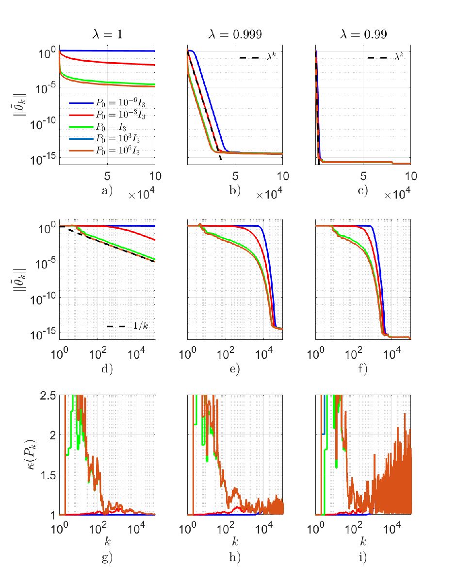
To apply RLS, let $\theta=[1\ 0.8\ 0.5]$ , $\theta_{0}=0$ , and $\phi_{k}=[u_{k-1}\ u_{k-2}\ u_{k-3}]$ , where the input $u_{k}$ is zero-mean Gaussian white noise with standard deviation 1. Note that $(\phi_{k})_{k=0}^{\infty}$ is persistently exciting. It thus follows from Theorem 7 that $\tilde{\theta}_{k}$ converges to zero. Figure 5 shows the parameter-error norm $\|\tilde{\theta}_{k}\|$ for several values of $P_{0}$ and $\lambda$ as well as the condition number of the corresponding $P_{k}$ . Note that the convergence rate of $\|\tilde{\theta}_{k}\|$ is $O(1/k)$ for $\lambda=1$ and geometric for all $\lambda\in(0,1)$ . Furthermore, as $\lambda$ is decreased, the convergence rate of $\theta_{k}$ increases; however, the condition number of $P_{k}$ degrades, and the effect of $P_{0}$ is reduced. $\diamond$

Lack of Persistent Excitation

This section presents numerical examples to investigate the effect of lack of persistent excitation. As shown in Example 3 and Example 5, if $(\phi_{k})_{k=0}^{\infty}$ is not persistently exciting and $\lambda=1$ , then some of the singular values of $P_{k}$ converge to zero, whereas the remaining singular values remain bounded. On the other hand, if $(\phi_{k})_{k=0}^{\infty}$ is not persistently exciting and $\lambda\in(0,1)$ , then some of the singular values of $P_{k}$ remain bounded, whereas the remaining singular values diverge. Furthermore, Proposition 6 implies that the predicted error $z_{k}$ converges to zero whether or not $(\phi_{k})_{k=0}^{\infty}$ is persistent.

Example 7

Lack of persistent excitation in scalar estimation. Let $n=1$ , so that (4), (5) are given by

	$\displaystyle P_{k+1}$	$\displaystyle=\dfrac{P_{k}}{\lambda+P_{k}\phi_{k}^{2}},$		(52)
	$\displaystyle\tilde{\theta}_{k+1}$	$\displaystyle=\dfrac{\lambda\tilde{\theta}_{k}}{\lambda+P_{k}\phi_{k}^{2}}.$		(53)

Now, let $k_{0}\geq 0$ and assume that, for all $k\geq k_{0},$ $\phi_{k}=0.$ Therefore, for all $j\geq 0$ and $N\geq 1,$ $F_{j,j+N}$ cannot be lower bounded as in (19), and thus $(\phi_{k})_{k=0}^{\infty}$ is not persistently exciting. Furthermore, in the case where $\lambda=1$ , it follows from the fact that $\phi_{k}=0$ for all $k\geq k_{0}$ that $P_{k}$ and $\tilde{\theta}_{k}$ converge in $k_{0}$ steps to $\overline{P}\neq 0$ and $\overline{\tilde{\theta}}$ , respectively. Furthermore, if $\theta_{0}\neq\theta,$ then $\overline{\tilde{\theta}}\neq 0.$ However, in the case where $\lambda\in(0,1)$ , it follows that $P_{k}$ diverges geometrically, whereas, as in the case where $\lambda=1,$ $\tilde{\theta}_{k}$ converges in $k_{0}$ steps. Therefore, for all $\lambda\in(0,1],$ since $\phi_{k}=0$ for all $k\geq k_{0},$ it follows from (52) and (53) that, for all $k\geq k_{0},$ the minimum value of (2) is achieved in a finite number of steps. Consequently, RLS provides no further refinement of the estimate $\theta_{k}$ of $\theta,$ and thus $\overline{\tilde{\theta}}\neq 0$ implies that $\theta_{k}$ does not converge to $\theta.$

Alternatively, assume that, for all $k\geq 0,$ $\phi_{k}=\overline{\phi},$ where $\overline{\phi}\neq 0$ . Then it follows from Definition 1 with $N=1$ , $\alpha=\overline{\phi}^{2}$ , and $\beta=3\overline{\phi}^{2}$ that $(\phi_{k})_{k=0}^{\infty}$ is persistently exciting. If $\lambda=1$ , then both $P_{k}$ and $\tilde{\theta}_{k}$ converge to zero. However, if $\lambda\in(0,1)$ , then $P_{k}$ converges to $\tfrac{1-\lambda}{\overline{\phi}^{2}}$ and $\tilde{\theta}_{k}$ converges geometrically to zero. Table 5 shows the asymptotic behavior of $\tilde{\theta}_{k}$ and $P_{k}$ for both of these cases. $\diamond$

Excitation $\backslash$ $\lambda$	$\lambda=1$	$\lambda\in(0,1)$
Not persistently exciting	$\tilde{\theta}_{k}\to\overline{\tilde{\theta}},P_{k}\to\overline{P}$	$\tilde{\theta}_{k}\to\overline{\tilde{\theta}},P_{k}$ diverges
Persistently exciting	$\tilde{\theta}_{k}\to 0,P_{k}\to 0$	$\tilde{\theta}_{k}\to 0,P_{k}\to\tfrac{1-\lambda}{\overline{\phi}^{2}}$

TABLE 5: Asymptotic behavior of RLS in Example 7. In the case of persistent excitation with

\lambda<1,

the convergence of

\tilde{\theta}_{k}

is geometric.

Example 8

Subspace-constrained regressor. Consider (1), where $\phi_{k}=(\sin\tfrac{2\pi k}{100})[1\ 1]$ and $\theta=[0.4\ 1.4]^{\rm T}$ . To estimate $\theta$ using RLS, let $P_{0}=I_{2}$ and $\theta_{0}=0$ . Figure 6 shows the estimate $\theta_{k}$ of $\theta$ with $\lambda=1$ and $\lambda=0.99$ . Note that all regressors $\phi_{k}$ lie along the same one-dimensional subspace, and thus, $(\phi_{k})_{k=0}^{\infty}$ is not persistently exciting. It follows from (16) that the estimate $\theta_{k}$ of $\theta$ lies in this subspace.

For $\lambda=1$ , note that one singular value decreases to zero, whereas the other singular value is bounded. Note that $\tilde{\theta}_{k}$ converges along the singular vector corresponding to the bounded singular value. For $\lambda=0.99,$ one singular value is bounded, whereas the other singular value diverges. Note that $\tilde{\theta}_{k}$ converges along the singular vector corresponding to the diverging singular value. $\diamond$

Example 9

Lack of persistent excitation and finite-precision arithmetic. Consider the problem of fitting a 5th-order model to measured input-output data from the system (34), where the input $u_{k}$ is given by (27). Note that $\phi_{k}$ is given by (35), and is not persistently exciting as shown in Example 5. Let $P_{0}=I_{10}$ , $\theta_{0}=0$ , and $\lambda=0.999$ . Figure 7 shows the predicted error $z_{k}$ , the norm of the parameter error $\tilde{\theta}_{k}$ , and the singular values and the condition number of $P_{k}$ . Note that the $\tilde{\theta}_{k}$ does not converge to zero and that six singular values of $P_{k}$ remain bounded due to the presence of three harmonics in the regresssor. Due to finite-precision arithmetic, the computation becomes erroneous as $P_{k}$ becomes numerically ill-conditioned, and thus the estimate $\theta_{k}$ diverges. $\diamond$

The numerical examples in this section show that, if $\lambda\in(0,1]$ and $(\phi_{k})_{k=0}^{\infty}$ is not persistently exciting, then $\tilde{\theta}_{k}$ does not necessarily converge to zero. Furthermore, if $\lambda\in(0,1)$ and $(\phi_{k})_{k=0}^{\infty}$ is not persistently exciting, then some of the singular values of $P_{k}$ diverge, and $\theta_{k}$ diverges due to finite-precision arithmetic when $P_{k}$ becomes numerically ill-conditioned.

Information Subspace

Using the singular value decomposition, (8) can be written as

\displaystyle P_{k+1}^{-1}=\lambda U_{k}\Sigma_{k}U_{k}^{\rm T}+U_{k}\psi_{k}^{\rm T}\psi_{k}U_{k}^{\rm T},

(54)

where $U_{k}\in{\mathbb{R}}^{n\times n}$ is an orthonormal matrix whose columns are the singular vectors of $P_{k}^{-1}$ , $\Sigma_{k}\in{\mathbb{R}}^{n\times n}$ is a diagonal matrix whose diagonal entries are the corresponding singular values, and

\displaystyle\psi_{k}\stackrel{{\scriptstyle\triangle}}{{=}}\phi_{k}U_{k}.

(55)

The columns of $U_{k}$ are the information directions at step $k$ , and each row of $\psi_{k}$ is the projection of the corresponding row of $\phi_{k}$ onto the information directions. The norm of each column of $\psi_{k}$ thus indicates the information content present in $\phi_{k}$ along the corresponding information direction. The smallest subspace that is spanned by a subset of the information directions and that contains all rows of $\phi_{k}$ is the information-rich subspace ${\mathcal{I}}_{k}$ at step $k$ . Figure 8 illustrates the information-rich subspace.

Now, consider the case where

\displaystyle\psi_{k}=\left[\begin{array}[]{cc}\psi_{k,1}&0_{p\times(n-n_{1})}\end{array}\right],

where $\psi_{k,1}\in{\mathbb{R}}^{p\times n_{1}}$ . It follows from (Information Subspace) that $\phi_{k}$ provides new information along the first $n_{1}$ columns of $U_{k}$ ; these directions constitute the information-rich subspace. It thus follows from (54) and (Information Subspace) that $P_{k+1}^{-1}$ is given by

\displaystyle P_{k+1}^{-1}=U_{k}\left[\begin{array}[]{cc}\lambda\Sigma_{k,1}+\psi_{k,1}^{\rm T}\psi_{k,1}&0\\ 0&\lambda\Sigma_{k,2}\end{array}\right]U_{k}^{\rm T},

where $\Sigma_{k,1}\in{\mathbb{R}}^{n_{1}\times n_{1}}$ is the diagonal matrix whose diagonal entries are the first $n_{1}$ singular values of $P_{k}^{-1}$ , and $\Sigma_{k,2}$ is the diagonal matrix whose diagonal entries are the remaining $n-n_{1}$ singular values of $P_{k}^{-1}$ . In particular, writing

\displaystyle U_{k}=\left[\begin{array}[]{cc}U_{k,1}&U_{k,2}\end{array}\right],

where $U_{k,1}\in{\mathbb{R}}^{n\times n_{1}}$ contains the first $n_{1}$ columns of $U_{k}$ , and $U_{k,2}\in{\mathbb{R}}^{n\times n-n_{1}}$ contains the remaining $n-n_{1}$ columns of $U_{k}$ , it follows that

\displaystyle P_{k+1}^{-1}=\left[\begin{array}[]{cc}U_{k+1,1}&U_{k+1,2}\end{array}\right]\left[\begin{array}[]{cc}\Sigma_{k+1,1}&0\\ 0&\Sigma_{k+1,2}\end{array}\right]\left[\begin{array}[]{c}U_{k+1,1}^{\rm T}\\ U_{k+1,2}^{\rm T}\end{array}\right],

where

$\displaystyle U_{k+1,1}$	$\displaystyle=U_{k,1}V_{k},$	(65)
$\displaystyle\Sigma_{k+1,1}$	$\displaystyle=D_{k},$	(66)
$\displaystyle U_{k+1,2}$	$\displaystyle=U_{k,2},$	(67)
$\displaystyle\Sigma_{k+1,2}$	$\displaystyle=\lambda\Sigma_{k,2},$	(68)

where $V_{k}\in{\mathbb{R}}^{n_{1}\times n_{1}}$ contains the singular vectors of $\lambda\Sigma_{k,1}+\psi_{k,1}^{\rm T}\psi_{k,1}$ and $D_{k}\in{\mathbb{R}}^{n_{1}\times n_{1}}$ is the diagonal matrix containing the corresponding singular values. It follows from (67), (68) that if, for all $k\geq 0$ , $\psi_{k}$ is given by (Information Subspace) and $\lambda\in(0,1)$ , then the last $n-n_{1}$ singular vectors of $P_{k}^{-1}$ do not change and the corresponding singular values of $P_{k}^{-1}$ decrease to zero geometrically. It thus follows from Proposition 4 that $(\phi_{k})_{k=0}^{\infty}$ is not persistently exciting. Furthermore, since $P_{k}$ and $P_{k}^{-1}$ have the same singular vectors and the singular values of $P_{k}$ are the reciprocals of the singular values of $P_{k}^{-1}$ , it follows that the last $n-n_{1}$ singular values of $P_{k}$ diverge.

The next example considers the case where there exists a proper subspace ${\mathcal{S}}\subset{\mathbb{R}}^{n}$ such that, for all $k\geq 0,$ ${\mathcal{R}}(\phi_{k}^{\rm T})\subseteq{\mathcal{S}}$ . Hence, $(\phi_{k})_{k=0}^{\infty}$ is not persistently exciting. In this case, for all $k\geq 0,$ the information-rich subspace ${\mathcal{I}}_{k}$ is a proper subspace of ${\mathbb{R}}^{n},$ and the singular values of $P_{k}^{-1}$ corresponding to the singular vectors in the orthogonal complement of ${\mathcal{I}}_{k}$ converge to zero.

Example 10

Lack of persistent excitation and the information-rich subspace. Consider the regressor $\phi_{k}$ given by (35) used in Example 5. Recall that $(\phi_{k})_{k=0}^{\infty}$ is not persistently exciting. Let $P_{0}=I_{10}$ . Figure 9 shows the information content $|\psi_{k,(i)}|$ for several values of $\lambda$ along with the singular values of the corresponding $P_{k}^{-1}$ . Note that the information-rich subspace is six dimensional due to the presence of three harmonics in $u_{k}$ as shown by six relatively large components of $\psi_{k}$ and, in the case where $\lambda<1$ , the singular values that correspond to the singular vectors not in the information-rich subspace converge to zero in machine precision. $\diamond$

Variable-Direction forgetting

Examples 3, 5, 7, 8, and 9 show that some of the singular values of $P_{k}^{-1}$ converge to zero in the case where $\phi_{k}$ is not persistently exciting. To address this situation, (8) is modified by replacing the scalar forgetting factor $\lambda$ by a data-dependent forgetting matrix $\Lambda_{k}$ . Similar modifications are discussed in “Toward Matrix Forgetting”. In particular, $P_{k+1}^{-1}$ is redefined as

\displaystyle P_{k+1}^{-1}=\Lambda_{k}P_{k}^{-1}\Lambda_{k}+\phi_{k}^{{\rm T}}\phi_{k},

(69)

where $\Lambda_{k}$ is a positive-definite (and thus symmetric) matrix constructed below. Note that, for all $k\geq 0,$ $P_{k+1}^{-1}$ given by (69) is positive definite. Using the singular value decomposition, (69) can be written as

\displaystyle P_{k+1}^{-1}=\Lambda_{k}U_{k}\Sigma_{k}U_{k}^{\rm T}\Lambda_{k}+U_{k}\psi_{k}^{\rm T}\psi_{k}U_{k}^{\rm T},

(70)

where $U_{k}$ , $\Sigma_{k}$ , and $\psi_{k}$ are as defined in the previous section.

The objective is to apply forgetting to only those singular values of $P_{k}^{-1}$ that correspond to the singular vectors in the information-rich subspace, that is, forgetting is restricted to the subspace of $P_{k}^{-1}$ where sufficient new information is provided by $\phi_{k}$ . Specifically, forgetting is applied to those information directions where the information content is greater than $\varepsilon>0$ , where $\varepsilon$ should be selected to be larger than the noise to signal ratio or larger than the machine zero, if no noise is present. To do so, (70) is written as

\displaystyle P_{k+1}^{-1}=U_{k}\overline{\Lambda}_{k}\Sigma_{k}\overline{\Lambda}_{k}U_{k}^{\rm T}+U_{k}\psi_{k}^{\rm T}\psi_{k}U_{k}^{\rm T},

(71)

where $\overline{\Lambda}_{k}$ is a diagonal matrix whose diagonal entries are either $\sqrt{\lambda}$ or $1$ . In particular,

\displaystyle\overline{\Lambda}_{k}(i,i)\stackrel{{\scriptstyle\triangle}}{{=}}\begin{cases}\sqrt{\lambda},&\|{\rm col}_{i}(\psi_{k})\|>\varepsilon,\\ 1,&\rm{otherwise},\end{cases}

(72)

where ${\rm col}_{i}(\psi_{k})$ is the $i$ th column of $\psi_{k}$ and $\lambda\in(0,1]$ . Note that, it follows from (71) and (72) that $P_{k+1}^{-1}$ is positive definite. Next, it follows from (70) and (71) that

\displaystyle\Lambda_{k}=U_{k}\overline{\Lambda}_{k}U_{k}^{\rm T},

(73)

which is positive definite. Note that

\displaystyle\Lambda_{k}^{-1}

\displaystyle=U_{k}\overline{\Lambda}_{k}^{-1}U_{k}^{\rm T}.

(74)

The next result provides a recursive formula to update $P_{k+1}$ given by (69).

Proposition 8

Let $\lambda\in(0,1]$ , $\varepsilon>0$ , let $(P_{k})_{k=0}^{\infty}$ be a sequence of $n\times n$ positive-definite matrices, and let $U_{k}\in{\mathbb{R}}^{n\times n}$ be an orthonormal matrix whose columns are the singular vectors of $P_{k}.$ Furthermore, let $\psi_{k}\in{\mathbb{R}}^{p\times n}$ be given by (55), let $\overline{\Lambda}_{k}$ be given by (72), and let $\Lambda_{k}$ be given by (73). Then, for all $k\geq 0,$ $(P_{k})_{k=0}^{\infty}$ satisfies (69) if and only if, for all $k\geq 0,$ $(P_{k})_{k=0}^{\infty}$ satisfies

\displaystyle P_{k+1}

\displaystyle=\overline{P}_{k}-\overline{P}_{k}\phi_{k}(I_{p}+\phi_{k}^{\rm T}\overline{P}_{k}\phi_{k})^{-1}\phi_{k}^{\rm T}\overline{P}_{k},

(75)

where

\displaystyle\overline{P}_{k}

\displaystyle=\Lambda_{k}^{-1}P_{k}\Lambda_{k}^{-1}.

(76)

Proof:

To prove necessity, it follows from (69) and matrix-inversion lemma, that

	$\displaystyle P_{k+1}$	$\displaystyle=(\Lambda_{k}P_{k}^{-1}\Lambda_{k}+\phi_{k}^{\rm T}\phi_{k})^{-1}$
		$\displaystyle=(\Lambda_{k}P_{k}^{-1}\Lambda_{k})^{-1}-(\Lambda_{k}P_{k}^{-1}\Lambda_{k})^{-1}\phi_{k}^{\rm T}[I_{p}+\phi_{k}(\Lambda_{k}P_{k}^{-1}\Lambda_{k})^{-1}\phi_{k}^{\rm T}]^{-1}\phi_{k}(\Lambda_{k}P_{k}^{-1}\Lambda_{k})^{-1}$
		$\displaystyle=\overline{P}_{k}-\overline{P}_{k}\phi_{k}(I_{p}+\phi_{k}^{\rm T}\overline{P}_{k}\phi_{k})^{-1}\phi_{k}^{\rm T}\overline{P}_{k},$

where $\overline{P}_{k}$ is given by (76). Reversing these steps proves sufficiency. ∎

The modified update (69) is shown to be optimal for a specific cost function in “A Modified Quadratic Cost Function Supporting Variable-Direction RLS”.

Next, the matrix-forgetting scheme (69) is shown to prevent the singular values of $P_{k}$ from diverging. Consider the case where, for all $k\geq 0$ ,

\displaystyle\psi_{k}=\left[\begin{array}[]{cc}\psi_{k,1}&0\end{array}\right],

where $\psi_{k,1}\in{\mathbb{R}}^{p\times n_{1}}$ , that is, the information-rich subspace is spanned by the first $n_{1}$ columns of $U_{k}$ . It thus follows from (71) and (Proof:) that $P_{k+1}^{-1}$ is given by

\displaystyle P_{k+1}^{-1}=U_{k}\left[\begin{array}[]{cc}\lambda\Sigma_{k,1}+\psi_{k,1}^{\rm T}\psi_{k,1}&0\\ 0&\Sigma_{k,2}\end{array}\right]U_{k}^{\rm T}.

It follows from the $(2,2)$ block of (Proof:) that the last $n-n_{1}$ information directions and the corresponding singular values are not affected by $\phi_{k}$ . Furthermore, if $n_{1}=n$ , that is, new information is present in $\phi_{k}$ along every information direction, then forgetting is applied to all of the singular values of $P_{k}^{-1}$ , and thus variable-direction forgetting specializes to uniform-direction forgetting, that is, RLS with the update for $P_{k}$ given by (8).

The next result shows that, as in the case of uniform-direction forgetting, $z_{k}$ converges to zero with variable-direction forgetting for every choice of $\varepsilon>0$ , whether or not $(\phi_{k})_{k=0}^{\infty}$ is persistently exciting.

Proposition 9

\displaystyle\lim_{k\to\infty}z_{k}=0.

(80)

Proof:

Using (72), (73), and $P_{k}^{-1}=U_{k}\Sigma_{k}U_{k}^{\rm T}$ , it follows that, for all $k\geq 0$ ,

\displaystyle\Lambda_{k}P_{k}^{-1}\Lambda_{k}

\displaystyle=U_{k}\overline{\Lambda}_{k}\Sigma_{k}\overline{\Lambda}_{k}U_{k}^{\rm T}\leq U_{k}\Sigma_{k}U_{k}^{\rm T}=P_{k}^{-1}.

(81)

	$\displaystyle V_{k+1}-V_{k}$	$\displaystyle=\tilde{\theta}_{k+1}^{\rm T}P_{k+1}^{-1}\tilde{\theta}_{k+1}-\tilde{\theta}_{k}^{\rm T}P_{k}^{-1}\tilde{\theta}_{k}$
		$\displaystyle=\tilde{\theta}_{k}^{\rm T}\Lambda_{k}P_{k}^{-1}\Lambda_{k}P_{k+1}\Lambda_{k}P_{k}^{-1}\Lambda_{k}\tilde{\theta}_{k}-\tilde{\theta}_{k}^{\rm T}P_{k}^{-1}\tilde{\theta}_{k}$
		$\displaystyle=\tilde{\theta}_{k}^{\rm T}[\Lambda_{k}P_{k}^{-1}\Lambda_{k}P_{k+1}\Lambda_{k}P_{k}^{-1}\Lambda_{k}-P_{k}^{-1}]\tilde{\theta}_{k}$
		$\displaystyle=\tilde{\theta}_{k}^{\rm T}[\Lambda_{k}P_{k}^{-1}(P_{k}-P_{k}\Lambda_{k}^{-1}\phi_{k}(I_{p}+\phi_{k}^{\rm T}\overline{P}_{k}\phi_{k})^{-1}\phi_{k}^{\rm T}\Lambda_{k}^{-1}P_{k})P_{k}^{-1}\Lambda_{k}-P_{k}^{-1}]\tilde{\theta}_{k}$
		$\displaystyle=\tilde{\theta}_{k}^{\rm T}[\Lambda_{k}P_{k}^{-1}\Lambda_{k}-\phi_{k}(I_{p}+\phi_{k}^{\rm T}\overline{P}_{k}\phi_{k})^{-1}\phi_{k}^{\rm T}-P_{k}^{-1}]\tilde{\theta}_{k}$
		$\displaystyle=-[\tilde{\theta}_{k}^{\rm T}(P_{k}^{-1}-\Lambda_{k}P_{k}^{-1}\Lambda_{k})\tilde{\theta}_{k}+z_{k}(I_{p}+\phi_{k}^{\rm T}\overline{P}_{k}\phi_{k})^{-1}z_{k}]$
		$\displaystyle\leq 0.$

Note that, since $(V_{k})_{k=1}^{\infty}$ is a nonnegative, nonincreasing sequence, it converges to a nonnegative number. Hence, $\lim_{k\to\infty}(V_{k+1}-V_{k})=0,$ which implies that lim_k→∞ [ ~ θ _k^T(P_k^-1 - Λ_k P_k^-1 Λ_k ) ~ θ _k + z_k (I_p+ϕ_k^TP_k ϕ_k)^-1 z_k ] = 0. Since, for all $k\geq 0$ , $P_{k}^{-1}-\Lambda_{k}P_{k}^{-1}\Lambda_{k}\geq 0$ and $(I_{p}+\phi_{k}^{\rm T}\overline{P}_{k}\phi_{k})^{-1}>0$ , it follows that $\lim_{k\to\infty}z_{k}=0.$ ∎

The next result shows that $P_{k}$ is bounded from above with variable-direction forgetting for every choice of $\varepsilon>0$ in the case where $(\phi_{k})_{k=0}^{\infty}$ is persistently exciting.

Proposition 10

\displaystyle\frac{\lambda^{N}(1-\lambda)\alpha}{1-\lambda^{N+1}}I_{n}\leq P_{k}^{-1}.

(82)

Proof:

It follows from (69), that, for all $k\geq 0,$ $\Lambda_{k}P_{k}^{-1}\Lambda_{k}\leq P_{k+1}^{-1}$ and $\phi_{k}^{\rm T}\phi_{k}\leq P_{k+1}^{-1}.$ Next, using (73) and $P_{k}^{-1}=U_{k}\Sigma_{k}U_{k}^{\rm T}$ , it follows that, for all $k\geq 0$ ,

\displaystyle\lambda P_{k}^{-1}

\displaystyle=\lambda U_{k}\Sigma_{k}U_{k}^{\rm T}\leq U_{k}\overline{\Lambda}_{k}\Sigma_{k}\overline{\Lambda}_{k}U_{k}^{\rm T}=\Lambda_{k}P_{k}^{-1}\Lambda_{k}\leq P_{k+1}^{-1}.

Finally, for all $k\geq N+1$ ,

	$\displaystyle\alpha I_{n}$	$\displaystyle\leq\sum_{i=k-N-1}^{k-1}\phi_{i}^{\rm T}\phi_{i}$
		$\displaystyle\leq\sum_{i=k-N}^{k}P_{i}^{-1}$
		$\displaystyle\leq(\lambda^{-N}+\cdots+1)P_{k}^{-1}$
		$\displaystyle=\dfrac{1-\lambda^{N+1}}{\lambda^{N}(1-\lambda)}P_{k}^{-1},$

which proves (82). ∎

The next two examples consider variable-direction forgetting in the case where $(\phi_{k})_{k=0}^{\infty}$ is not persistently exciting. In these examples, $P_{k}$ is bounded, $z_{k}$ converges to zero, and $\theta_{k}$ converges, although not to the true value $\theta.$

Example 11

Variable-direction forgetting for a regressor lacking persistent excitation. Reconsider Example 10. Let $P_{0}=I_{10}$ , and $P_{k}^{-1}$ be given by (75), where $\varepsilon=10^{-8}$ . Figure 10 shows the information content $|{\rm col}_{i}(\psi_{k})|$ and the singular values of the $P_{k}^{-1}$ for several values of $\lambda$ . Note that the information-rich subspace is six dimensional due to the presence of three harmonics in $u_{k}$ as shown by six relatively large components of $\psi_{k}$ and the singular values that correspond to the singular vectors not in the information-rich subspace do not converge to zero. $\diamond$

Example 12

Effect of variable-direction forgetting on $\theta_{k}$ . Reconsider Example 9. Let $P_{0}=I_{10}$ , and $P_{k}^{-1}$ be given by (75), where $\varepsilon=10^{-8}$ . Figure 11 shows the predicted error $z_{k}$ , the norm of the parameter error $\tilde{\theta}_{k}$ , and the singular values and the condition number of $P_{k}$ . Note that the $\tilde{\theta}_{k}$ does not converge to zero and, unlike uniform-direction forgetting, all of the singular values of $P_{k}$ remain bounded and $\theta_{k}$ is bounded. $\diamond$

Concluding Remarks

This tutorial article presented a self-contained exposition of uniform-direction and variable-direction forgetting within the context of RLS. It was shown that, in the case of persistent excitation without forgetting, the parameter estimates converge asymptotically, whereas, with forgetting, the parameter estimates converge geometrically. Numerical examples were presented to illustrate this behavior.

In the case where forgetting is used but the excitation is not persistent, it was shown that forgetting is enforced in all information directions, whether or not new information is present along these directions. Consequently, the parameter estimates converge, but not necessarily to their true values; furthermore, the matrix $P_{k}$ diverges, leading to numerical instability. This phenomenon was traced to the divergence of the singular values of $P_{k}$ corresponding to singular vectors that are orthogonal to the information-rich subspace.

In order to address this problem, a data-dependent forgetting matrix was constructed to restrict forgetting to the information-rich subspace. The RLS cost function that corresponds to this extension of RLS was presented. Numerical examples showed that this variable-direction forgetting technique prevents $P_{k}$ from diverging under lack of persistent excitation.

Since RLS is fundamentally least squares optimization, its estimates are not consistent in the case of sensor noise [37]. An open problem is thus to develop extensions of RLS that provide consistent parameter estimates in the presence of errors-in-variable noise arising in system identification problems [38].

Acknowledgments

This research was partially supported by AFOSR under DDDAS grant FA9550-16-1-0071 (Dynamic Data-Driven Applications Systems http://www.1dddas.org/).

References

[1] M. Grewal and K. Glover, “Identifiability of linear and nonlinear dynamical systems,” IEEE Trans. Autom. Contr., vol. 21, no. 6, pp. 833–837, 1976.
[2] I. Y. Mareels and M. Gevers, “Persistence of excitation criteria,” in Proc. Conf. Dec. Contr, 1986, pp. 1933–1935.
[3] I. M. Mareels, R. R. Bitmead, M. Gevers, C. R. Johnson, and R. L. Kosut, “How exciting can a signal really be?” Sys. Contr. Lett., vol. 8, no. 3, pp. 197–204, 1987.
[4] I. M. Mareels and M. Gevers, “Persistency of excitation criteria for linear, multivariable, time-varying systems,” Mathematics of Control, Signals, and Systems, vol. 1, no. 3, pp. 203–226, 1988.
[5] B. D. O. Anderson, “Adaptive systems, lack of persistency of excitation and bursting phenomena,” Automatica, vol. 21, no. 3, pp. 247–258, 1985.
[6] G. Chowdhary and E. Johnson, “Concurrent learning for convergence in adaptive control without persistency of excitation,” in Proc. Conf. Dec. Contr., 2010, pp. 3674–3679.
[7] G. Chowdhary, M. Mühlegg, and E. Johnson, “Exponential parameter and tracking error convergence guarantees for adaptive controllers without persistency of excitation,” Int. J. Contr., vol. 87, no. 8, pp. 1583–1603, 2014.
[8] S. Aranovskiy, A. Bobtsov, R. Ortega, and A. Pyrkin, “Performance enhancement of parameter estimators via dynamic regressor extension and mixing,” IEEE Trans. Autom. Contr., vol. 62, no. 7, pp. 3546–3550, 2017.
[9] P. Panda, J. M. Allred, S. Ramanathan, and K. Roy, “Learning to forget with adaptive synaptic plasticity in spiking neural networks,” J. Emerg. Selec. Top. Circ. Syst., vol. 8, no. 1, pp. 51–64, 2018.
[10] J. M. Allred and K. Roy, “Unsupervised incremental stdp learning using forced firing of dormant or idle neurons,” in 2016 International Joint Conference on Neural Networks, July 2016, pp. 2492–2499.
[11] N. Frémaux and W. Gerstner, “Neuromodulated spike-timing-dependent plasticity, and theory of three-factor learning rules,” Frontiers in Neural Circuits, vol. 9, pp. 85–103, 2016.
[12] B. Han, A. Ankit, A. Sengupta, and K. Roy, “Cross-layer design exploration for energy-quality tradeoffs in spiking and non-spiking deep artificial neural networks,” IEEE Transactions on Multi-Scale Computing Systems, 2017.
[13] S. A. U. Islam and D. S. Bernstein, “Recursive Least Squares for Real-Time Implementation,” IEEE Contr. Sys. Mag., vol. 39, pp. 82–85, June 2019.
[14] L. Ljung, System Identification: Theory for the User, 2nd ed. Prentice Hall, 1999.
[15] A. H. Sayed, Fundamentals of Adaptive Filtering. Wiley, 2003.
[16] K. J. Astrom and B. Wittenmark, Computer-Controlled Systems: Theory and Design, 3rd ed. Prentice-Hall, 1996.
[17] T. R. Fortescue, L. S. Kershenbaum, and B. E. Ydstie, “Implementation of Self-tuning Regulators with Variable Forgetting Factors,” Automatica, vol. 17, no. 6, pp. 831–835, 1981.
[18] C. Paleologu, J. Benesty, and C. Silviu, “A Robust Variable Forgetting Factor Recursive Least-Squares Algorithm for System Identification,” IEEE Sig. Proc. Lett., vol. 15, pp. 597–600, 2008.
[19] S.-H. Leung and C. F. So, “Gradient-Based Variable Forgetting Factor RLS Algorithm in Time-Varying Environments,” IEEE Trans. Sig. Proc., vol. 53, no. 8, pp. 3141–3150, 2005.
[20] S. Song, J.-S. Lim, S. J. Baek, and K.-M. Sung, “Gauss Newton variable forgetting factor recursive least squares for time varying parameter tracking,” Electron. Lett., vol. 36, no. 11, pp. 988–990, 2000.
[21] D. J. Park, B. E. Jun, and K. J. H., “Fast tracking RLS algorithm using novel variable forgetting factor with unity zone,” Electron. Lett., vol. 27, no. 23, pp. 2150–2151, 1991.
[22] A. A. Ali, J. B. Hoagg, M. Mossberg, and D. S. Bernstein, “On the stability and convergence of a sliding-window variable-regularization recursive-least-squares algorithm,” Int. J. Adapt. Contr. Sig. Proc., vol. 30, pp. 715–735, 2016.
[23] R. M. Canetti and M. D. España, “Convergence analysis of the least-squares identification algorithm with a variable forgetting factor for time-varying linear systems,” Automatica, vol. 25, no. 4, pp. 609–612, 1989.
[24] M. E. Salgado, G. C. Goodwin and R. H. Middleton, “Modified least squares algorithm incorporating exponential resetting and forgetting,” Int. J. Contr., vol. 47, no. 2, pp. 477–491, 1988.
[25] G. Goodwin, E. Teoh, and H. Elliott, “Deterministic convergence of a self-tuning regulator with covariance resetting,” in IEE Proceedings D-Control Theory and Applications, vol. 130, no. 1, 1983, pp. 6–8.
[26] R. Kulhavỳ, “Restricted exponential forgetting in real-time identification,” Automatica, vol. 23, no. 5, pp. 589–600, 1987.
[27] R. Kulhav\‘y and M. Kárn\‘y, “Tracking of slowly varying parameters by directional forgetting,” IFAC Proc. Vol., vol. 17, no. 2, pp. 687–692, 1984.
[28] G. Kreisselmeier, “Stabilized least-squares type adaptive identifiers,” IEEE Trans. Autom. Contr., vol. 35, no. 3, pp. 306–310, 1990.
[29] L. Cao and H. Schwartz, “Directional forgetting algorithm based on the decomposition of the information matrix,” Automatica, vol. 36, no. 11, pp. 1725–1731, 2000.
[30] G. Kubin, “Stabilization of the RLS algorithm in the absence of persistent excitation,” in Proc. Int. Conf. Acoustics, Speech, Signal Processing, 1988, pp. 1369–1372.
[31] S. Bittanti, P. Bolzern, and M. Campi, “Convergence and exponential convergence of identification algorithms with directional forgetting factor,” Automatica, vol. 26, no. 5, pp. 929–932, 1990.
[32] ——, “Exponential convergence of a modified directional forgetting identification algorithm,” Sys. Contr. Lett., vol. 14, no. 2, pp. 131–137, 1990.
[33] A. Goel and D. S. Bernstein, “A targeted forgetting factor for recursive least squares,” in Proc. Conf. Dec. Contr., 2018, pp. 3899–3903.
[34] R. M. Johnstone, C. R. Johnson, R. R. Bitmead, and B. D. O. Anderson, “Exponential convergence of recursive least squares with exponential forgetting factor,” in Proc. Conf. Dec. Contr., 1982, pp. 994–997.
[35] J. Benesty and T. Gänsler, “New Insights into the RLS Algorithm,” Eurasip Jour. App. Sig. Proc., no. 3, pp. 331–339, 2004.
[36] W. M. Haddad and V. Chellaboina, Nonlinear Dynamical Systems and Control: A Lyapunov-based Approach. Princeton University Press, 2008.
[37] P. Eykhoff, System Identification: Parameter and State Estimation. Wiley-Interscience, 1974.
[38] T. Söderström, Errors-in-variables methods in system identification. Springer, 2018.

Sidebar: Summary

Learning depends on the ability to acquire and assimilate new information. This ability depends—somewhat counterintuitively—on the ability to forget. In particular, effective forgetting requires the ability to recognize and utilize new information to order to update a system model. This article is a tutorial on forgetting within the context of recursive least squares (RLS). To do this, RLS is first presented in its classical form, which employs uniform-direction forgetting. Next, examples are given to motivate the need for variable-direction forgetting, especially in cases where the excitation is not persistent. Some of these results are well known, whereas others complement the prior literature. The goal is to provide a self-contained tutorial of the main ideas and techniques for students and researchers whose research may benefit from variable-direction forgetting.

Sidebar: Three Useful Lemmas

Lemma 1

Let $X\in{\mathbb{R}}^{n\times p}$ and $y\in{\mathbb{R}}^{n}$ , and let $W\in{\mathbb{R}}^{p\times p}$ be positive definite. Then,

\displaystyle(I_{n}+XWX^{\rm T})^{-1}y\in{\mathcal{R}}([X\ \ y]).

(S1)

Proof:

Note that

	$\displaystyle y$	$\displaystyle\in{\mathcal{R}}([X\ \ y])$
		$\displaystyle={\mathcal{R}}[X\ \ y+XWX^{\rm T}y]$
		$\displaystyle={\mathcal{R}}\left([X\ \ (I_{n}+XWX^{\rm T})y]\left[\begin{array}[]{cc}I_{p}+WX^{\rm T}X&0\\ 0&1\end{array}\right]\right)$
		$\displaystyle={\mathcal{R}}([X(I_{p}+WX^{\rm T}X)\ \ (I_{n}+XWX^{\rm T})y])$
		$\displaystyle={\mathcal{R}}([(I_{n}+XWX^{\rm T})X\ \ (I_{n}+XWX^{\rm T})y])$
		$\displaystyle=(I_{n}+XWX^{\rm T}){\mathcal{R}}([X\ \ y]),$

which implies (S1). ∎

Lemma 2

Let $A\in{\mathbb{R}}^{n\times n}$ be positive semidefinite, and let $\lambda>0$ . Then,

\displaystyle I_{n}-A(\lambda I_{n}+A)^{-1}>0.

(S4)

Proof:

Write $A=SDS^{\rm T}$ , where $D={\rm diag}(d_{1},\ldots,d_{n})$ is diagonal and $S$ is unitary. For all $i\in\{1,\ldots,n\},$ $d_{i}\geq 0,$ and thus $\tfrac{d_{i}}{\lambda+d_{i}}<1$ . Hence,

\displaystyle D(\lambda I_{n}+D)^{-1}={\rm diag}\left(\tfrac{d_{1}}{\lambda+d_{1}},\ldots,\tfrac{d_{n}}{\lambda+d_{n}}\right)<I_{n}.

(S5)

Pre-multiplying and post-multiplying (S5) by $S$ and $S^{\rm T}$ , respectively, yields (S4). ∎

Lemma 3

Let $A\in{\mathbb{R}}^{n\times n}$ be positive semidefinite, and let $\lambda>0$ . Then,

\displaystyle I_{n}-\dfrac{1}{\lambda}\left(A-A(\lambda I_{n}+A)^{-1}A\right)>0.

(S6)

Proof:

Write $A=SDS^{\rm T}$ , where $D={\rm diag}(d_{1},\ldots,d_{n})$ is diagonal and $S$ is unitary. For all $i\in\{1,\ldots,n\},$ $d_{i}\geq 0,$ and thus $\tfrac{d_{i}}{\lambda+d_{i}}<1$ . Hence,

\displaystyle\dfrac{1}{\lambda}\left(D-D(\lambda I_{n}+D)^{-1}D\right)={\rm diag}\left(\tfrac{d_{1}}{\lambda+d_{1}},\ldots,\tfrac{d_{n}}{\lambda+d_{n}}\right)<I_{n}.

(S7)

Pre-multiplying and post-multiplying (S7) by $S$ and $S^{\rm T}$ , respectively, yields (S6). ∎

Sidebar: RLS as a One-Step Optimal Predictor

Consider the linear system

	$\displaystyle x_{k+1}$	$\displaystyle=A_{k}x_{k}+B_{k}u_{k}+w_{1,k},$		(S1)
	$\displaystyle y_{k}$	$\displaystyle=C_{k}x_{k}+w_{2,k},$		(S2)

where, for all $k\geq 0,$ $x_{k}\in{\mathbb{R}}^{n}$ , $u_{k}\in{\mathbb{R}}^{m}$ , $y_{k}\in{\mathbb{R}}^{p}$ , and $A_{k},B_{k},C_{k}$ are real matrices of appropriate sizes. The input $u_{k}$ and output $y_{k}$ are assumed to be measured. The process noise $w_{1,k}\in{\mathbb{R}}^{n}$ and the sensor noise $w_{2,k}\in{\mathbb{R}}^{p}$ are zero-mean white noise processes with variances ${\mathbb{E}}[w_{1,k}w_{1,k}^{\rm T}]=Q_{k}$ and ${\mathbb{E}}[w_{2,k}w_{2,k}^{\rm T}]=R_{k}$ , respectively. The expected value of the initial state is assumed to be $\overline{x}_{0}$ , and the variance of the initial state is $P_{0}$ , that is, ${\mathbb{E}}[x_{0}]=\overline{x}_{0}$ and ${\mathbb{E}}[(x_{0}-\overline{x}_{0})(x_{0}-\overline{x}_{0})^{\rm T}]=P_{0}$ . The objective is to estimate the state $x_{k}$ given the measurements of $u_{k}$ and $y_{k}$ .

To estimate $x_{k}$ , consider the estimator

\displaystyle\hat{x}_{k+1}

\displaystyle=A_{k}\hat{x}_{k}+B_{k}u_{k}+K_{k}(y_{k}-C_{k}\hat{x}_{k}),

(S3)

where $\hat{x}_{k}$ is the estimate of $x_{k}$ at step $k$ and $\hat{x}_{0}=\overline{x}_{0}$ . The matrix $K_{k}$ is constructed as follows. Define the state-estimate error $e_{k}\stackrel{{\scriptstyle\triangle}}{{=}}x_{k}-\hat{x}_{k}$ and the state error covariance $P_{k}\stackrel{{\scriptstyle\triangle}}{{=}}{\mathbb{E}}[e_{k}e_{k}^{\rm T}]\in{\mathbb{R}}^{n\times n}$ . Then, $e_{k}$ and $P_{k}$ satisfy

	$\displaystyle e_{k+1}$	$\displaystyle=(A_{k}-K_{k}C_{k})e_{k}+w_{1,k}-K_{k}w_{2,k},$		(S4)
	$\displaystyle P_{k+1}$	$\displaystyle=A_{k}P_{k}A_{k}^{\rm T}+Q_{k}+K_{k}\left(R_{k}+C_{k}P_{k}C_{k}^{\rm T}\right)K_{k}^{\rm T}-A_{k}P_{k}C_{k}^{\rm T}K_{k}^{\rm T}-C_{k}P_{k}A_{k}^{\rm T}.$		(S5)

Proposition S1

Let $P_{k+1}$ be given by (S5). The matrix $K_{k}$ that minimizes ${\rm tr\ }P_{k+1}$ is given by

\displaystyle K_{k}

\displaystyle=A_{k}P_{k}C_{k}^{\rm T}\left(R_{k}+C_{k}P_{k}C_{k}^{\rm T}\right)^{-1},

(S6)

and the minimized state-error covariance $P_{k}$ is updated as

\displaystyle P_{k+1}

\displaystyle=A_{k}P_{k}A_{k}^{\rm T}+Q_{k}-A_{k}P_{k}C_{k}^{\rm T}\left(R_{k}+C_{k}P_{k}C_{k}^{\rm T}\right)^{-1}C_{k}P_{k}A_{k}^{\rm T}.

(S7)

Proof:

See [S1]. ∎

Let $A_{k}=I_{n}$ , $B_{k}=0$ , $C_{k}=\phi_{k}$ , $Q_{k}=0,$ and $R_{k}=I_{p}$ . Then,

	$\displaystyle\hat{x}_{k+1}$	$\displaystyle=\hat{x}_{k}+P_{k}\phi_{k}^{\rm T}\left(I_{p}+\phi_{k}P_{k}\phi_{k}^{\rm T}\right)^{-1}(y_{k}-\phi_{k}\hat{x}_{k}),$		(S8)
	$\displaystyle P_{k+1}$	$\displaystyle=P_{k}-P_{k}\phi_{k}^{\rm T}\left(I_{p}+\phi_{k}P_{k}\phi_{k}^{\rm T}\right)^{-1}\phi_{k}P_{k}.$		(S9)

Note that (6), (7) with $\lambda=1$ have the same form as (S8), (S9). In particular, RLS without forgetting is the state estimator for the linear time-varying system with $A_{k}=I_{n}$ , $B_{k}=0$ , $C_{k}=\phi_{k}$ , $Q_{k}=0,$ and $R_{k}=I_{p}$ .

References

[S1] S. A. U. Islam, A. Goel, and D. S. Bernstein, “Real-Time Implementation of the Optimal Predictor and Optimal Filter: Accuracy versus Latency,” IEEE Contr. Sys. Mag., to appear.

Sidebar: RLS as a Maximum Likelihood Estimator

Let $k\geq 0$ and, for all $i\in\{0,1,\ldots,k\},$ consider the process

\displaystyle y_{i}=\phi_{i}\theta_{\rm true}+v_{i},

(S1)

where $\theta_{\rm true}\in{\mathbb{R}}^{n}$ is the unknown parameter, $\phi_{i}\in{\mathbb{R}}^{p\times n}$ is the regressor matrix, $v_{i}\in{\mathbb{R}}^{p}$ is the measurement noise, and $y_{i}\in{\mathbb{R}}^{p}$ is the measurement. The goal is to estimate $\theta_{\rm true}$ using the data $(\phi_{i})_{i=0}^{k}$ and $(y_{i})_{i=0}^{k}$ .

Let $\theta_{\rm true}$ be modeled by the $n$ -dimensional, real-valued normal random variable $\Theta$ with mean $\theta_{0}\in{\mathbb{R}}^{n}$ and covariance $(\lambda^{k+1}R)^{-1}$ , where $\lambda\in(0,1]$ and $R\in{\mathbb{R}}^{n\times n}$ is positive definite. For $\theta\in{\mathbb{R}}^{n},$ the density of $\Theta$ is thus given by

\displaystyle f_{\Theta}(\theta)=\dfrac{1}{\sqrt{(2\pi)^{n}{\rm det}\,{(\lambda^{k+1}R)^{-1}}}}{\rm exp}[-\tfrac{1}{2}(\theta-\theta_{0})^{\rm T}\lambda^{k+1}R(\theta-\theta_{0})].

(S2)

For all $i\in\{0,1,\ldots,k\}$ , assume that $v_{i}$ is a sample of the zero-mean, $p$ -dimensional, real-valued normal random variable $V_{i}$ with covariance $\lambda^{i-k}I_{p}$ . For $v_{i}\in{\mathbb{R}}^{p},$ the density of $V_{i}$ is thus given by

\displaystyle f_{V_{i}}(v_{i})=\dfrac{1}{\sqrt{(2\pi)^{p}\lambda^{i-k}}}{\rm exp}(-\tfrac{1}{2}v_{i}^{\rm T}\lambda^{k-i}I_{p}v_{i}).

(S3)

Assume that $V_{0},V_{1},\ldots,V_{k}$ are independent.

Since $\theta_{\rm true}$ and $v_{i}$ are modeled as normal random variables, it follows from (S1) that $y_{i}$ is a sample of the $p$ -dimensional, real-valued normal random variable $Y_{i}=\phi_{i}\theta_{\rm true}+V_{i}$ . Note that, since $V_{0},V_{1},\ldots,V_{k}$ are independent, it follows that $Y_{0},Y_{1},\ldots,Y_{k}$ are independent. Using (S1) and (S3), it thus follows that

\displaystyle f_{Y_{i}|\theta}(y_{i})=\dfrac{1}{\sqrt{(2\pi)^{p}\lambda^{i-k}}}{\rm exp}[-\tfrac{1}{2}(y_{i}-\phi_{k}\theta)^{\rm T}\lambda^{k-i}I_{p}(y_{i}-\phi_{k}\theta)],

(S4)

where $f_{Y_{i}|\theta}(y_{i})$ is the density of the random variable $Y_{i}$ conditions on $\Theta$ taking the value $\theta$ .

It follows from Bayes’ rule [S1, p. 413] that

\displaystyle f_{\Theta|\{y_{0},\ldots,y_{k}\}}(\theta)

\displaystyle=\alpha^{-1}f_{\Theta}(\theta)\prod_{i=0}^{k}f_{Y_{i}|\theta}(y_{i}),

(S5)

where

\displaystyle\alpha\stackrel{{\scriptstyle\triangle}}{{=}}\int_{{\mathbb{R}}^{n}}f_{\Theta}(\theta)\prod_{i=0}^{k}f_{Y_{i}|\theta}(y_{i})\,{\rm d}\theta.

(S6)

Substituting (S2) and (S4) into (S5), it follows that

\displaystyle f_{\Theta|\{y_{0},\ldots,y_{k}\}}(\theta)=\beta{\rm exp}\left[\sum_{i=0}^{k}-\tfrac{1}{2}\lambda^{k-i}(y_{i}-\phi_{k}\theta)^{\rm T}(y_{i}-\phi_{k}\theta)-\tfrac{1}{2}\lambda^{k+1}(\theta-\theta_{0})^{\rm T}R(\theta-\theta_{0})\right],

(S7)

where

\displaystyle\beta\stackrel{{\scriptstyle\triangle}}{{=}}\dfrac{1}{\alpha\sqrt{(2\pi)^{p}\lambda^{i-k}}}\dfrac{1}{\sqrt{(2\pi)^{n}{\rm det}\,{(\lambda^{k+1}R)^{-1}}}}.

(S8)

Finally, the maximum likelihood estimate of $\theta_{\rm true}$ is given by the maximizer of (S7), that is,

\displaystyle\theta_{{\rm ML}}=\underset{\theta\in{\mathbb{R}}^{n}}{\operatorname{argmax}}\ f_{\Theta|\{y_{0},\ldots,y_{k}\}}(\theta).

(S9)

In fact, $\theta_{\rm ML}=\underset{\theta\in{\mathbb{R}}^{n}}{\operatorname{argmin}}\ J_{k}(\theta)$ , where $J_{k}(\theta)$ is given by (2). Therefore, RLS with forgetting can be interpreted as the maximum likelihood estimator of the random variable $\Theta.$

References

[S1] D. P. Bertsekas, and J. N. Tsitsiklis. Introduction to Probability, Second Edition, Athena Scientific, 2008.

Sidebar: Toward Matrix Forgetting

In [S1], $P_{k}^{-1}$ is updated by

\displaystyle P_{k+1}^{-1}

\displaystyle=(I_{n}+M_{k}P_{k})P_{k}^{-1}+\phi_{k}^{\rm T}\phi_{k},

(S1)

where $M_{k}\in{\mathbb{R}}^{n\times n}$ is chosen to guarantee asymptotic stability and boundedness. Two choices of matrix $M_{k}$ are considered. In the first case,

\displaystyle M_{k}

\displaystyle\stackrel{{\scriptstyle\triangle}}{{=}}-(1-\lambda)(I-\alpha P_{k})^{N}P_{k}^{-1},

(S2)

where $\lambda\in(0,1)$ , $\alpha>0$ , and $N$ is an odd, positive integer. In the second case,

\displaystyle M_{k}

\displaystyle=-(1-\lambda)(P_{k}^{-1}-\alpha I_{n})^{N}(P_{k}^{-1}+\beta I_{n})^{-N}P_{k}^{-1},

(S3)

where $\lambda\in(0,1)$ , $\alpha>0$ , $\beta\geq 0$ , and $N$ is an odd, positive integer. Note that RLS with constant forgetting is obtained by setting $M_{k}=(\lambda-1)P_{k}^{-1}$ in (S1).

Proposition S1

Consider (S1) with (S2) or (S3). Let $P_{0}$ be symmetric and nonsingular. Then, the following statements hold:

$i)$

For all $k\geq 0$ , $P_{k}$ is symmetric and nonsingular.
$ii)$

If $P_{0}^{-1}\geq\tfrac{\alpha}{2}I_{n}$ , then, $P_{k}^{-1}=\alpha I$ is an asymptotically stable equilibrium of (S1).
$iii)$

If $P_{0}^{-1}\geq\alpha I_{n}$ , then, for all $k\geq 0$ , $P_{k}^{-1}\geq\alpha I_{n}$ .
$iv)$

If $P_{0}^{-1}\geq\alpha I_{n}$ and, for all $k\geq 0$ , $\phi_{k}$ is bounded, then $P_{k}^{-1}$ is bounded.
$v)$

If $P_{0}^{-1}\geq\alpha I_{n}$ and $\phi_{k}$ is persistently exciting, then there exists $k_{0}>0$ such that, for all $k\geq k_{0},$ $P_{k}^{-1}>\alpha I_{n}$ .

Proof:

See [28]. ∎

The main goal of (S1) is stabilization of $P_{k}$ in the case where $(\phi_{k})_{k=0}^{\infty}$ is not persistently exciting. Proposition S1 implies that $P_{k}$ remains bounded whether or not $(\phi_{k})_{k=0}^{\infty}$ is persistent. However, (S1) is not designed to implement forgetting. Furthermore, note that (S1) requires the computation of the inverse of an $n\times n$ matrix at each step.

An alternative directional forgetting scheme given in [S2] considers the update

\displaystyle P_{k+1}^{-1}

\displaystyle=M_{k}P_{k}^{-1}+\phi_{k}^{\rm T}\phi_{k},

(S4)

where $M_{k}\in{\mathbb{R}}^{n\times n}$ is designed to apply forgetting to a specific subspace. In the case of a scalar measurement, that is, $p=1$ , $P_{k}^{-1}$ is decomposed as

\displaystyle P_{k}^{-1}=P_{1,k}^{-1}+P_{2,k}^{-1},

(S5)

where $P_{1,k}^{-1}$ is chosen such that $P_{1,k}^{-1}\phi_{k}^{\rm T}=0$ , that is, $\phi_{k}^{\rm T}$ is in the null space of $P_{1,k}^{-1}$ . Next, forgetting is restricted to $P_{2,k}^{-1}$ , that is,

\displaystyle P_{k+1}^{-1}

\displaystyle=P_{1,k}^{-1}+\lambda P_{2,k}^{-1}+\phi_{k}^{\rm T}\phi_{k}.

(S6)

The matrix $P_{2,k}^{-1}$ is chosen to be positive semidefinite with rank $1$ by using

\displaystyle P_{2,k}^{-1}\stackrel{{\scriptstyle\triangle}}{{=}}P_{k}^{-1}\phi_{k}^{{\rm T}}\left(\phi_{k}P_{k}^{-1}\phi_{k}^{\rm T}\right)^{-1}\phi_{k}P_{k}^{-1},

(S7)

and thus $P_{1,k}^{-1}=P_{k}^{-1}-P_{2,k}^{-1}.$ Finally, it follows from (S4), (S6), and (S7) that

\displaystyle M_{k}=I_{n}-(1-\lambda)\left(\phi_{k}P_{k}^{-1}\phi_{k}^{\rm T}\right)^{-1}P_{k}^{-1}\phi_{k}^{\rm T}\phi_{k}

(S8)

and $P_{k+1}$ is computed as

	$\displaystyle\overline{P}_{k}$	$\displaystyle=\begin{cases}P_{k}+\dfrac{1-\lambda}{\lambda}\left(\phi_{k}P_{k}^{-1}\phi_{k}^{\rm T}\right)^{-1}\phi_{k}^{\rm T}\phi_{k},&\phi_{k}\neq 0,\\ P_{k},&\phi_{k}=0,\\ \end{cases}$		(S9)
	$\displaystyle P_{k+1}$	$\displaystyle=\overline{P}_{k}-\overline{P}_{k}\phi_{k}(1+\phi_{k}^{\rm T}\overline{P}_{k}\phi_{k})^{-1}\phi_{k}^{\rm T}\overline{P}_{k}.$		(S10)

It is shown in [S2] that, if $P_{k}^{-1}$ is positive definite, then, for all $\lambda\in(0,1]$ , $M_{k}P_{k}^{-1}$ is positive definite. Furthermore, if, for all $k\geq 0$ , $\phi_{k}$ is bounded, then there exists $\beta>0$ such that, for all $k\geq 0$ , $P_{k}<\beta I_{n}$ .

References

[S1] G. Kreisselmeier, “Stabilized least-squares type adaptive identifiers,” IEEE Trans. Autom. Contr., vol. 35, no. 3, pp. 306–310, 1990.
[S2] L. Cao and H. Schwartz, “Directional forgetting algorithm based on the decomposition ofthe information matrix,” Automatica, vol. 36, no. 11, pp. 1725–1731, 2000.

Sidebar: A Cost Function for Variable-Direction RLS

Theorem S1

For all $k\geq 0$ , let $\phi_{k}\in{\mathbb{R}}^{p\times n}$ and $y_{k}\in{\mathbb{R}}^{p}$ . Furthermore, let $R\in{\mathbb{R}}^{n\times n}$ be positive definite, let $\lambda\in(0,1],$ and, for all $k\geq 0,$ let $P_{k}$ be given by

\displaystyle P_{k+1}^{-1}=\Lambda_{k}P_{k}^{-1}\Lambda_{k}+\phi_{k}^{{\rm T}}\phi_{k},

(S1)

where $P_{0}\stackrel{{\scriptstyle\triangle}}{{=}}R^{-1}$ and let $\Lambda_{k}$ be given by (73). In addition, let $\theta_{0}\in{\mathbb{R}}^{n}$ , and define

\displaystyle J_{k}({\hat{\theta}})

\displaystyle\stackrel{{\scriptstyle\triangle}}{{=}}\sum_{i=0}^{k}(y_{i}-\phi_{i}{\hat{\theta}})^{\rm T}(y_{i}-\phi_{i}{\hat{\theta}})+({\hat{\theta}}-\theta_{0})^{\rm T}R_{k}({\hat{\theta}}-\theta_{0}),

(S2)

where, for all $k\geq 0$ ,

\displaystyle R_{k}=R_{k-1}+\Lambda_{k}P_{k}^{-1}\Lambda_{k}-P_{k}^{-1},

(S3)

where $R_{-1}\stackrel{{\scriptstyle\triangle}}{{=}}R$ . Then, for all $k\geq 0$ , (S2) has a unique global minimizer

\displaystyle\theta_{k+1}=\underset{\hat{\theta}\in{\mathbb{R}}^{n}}{\operatorname{argmin}}\ J_{k}({\hat{\theta}}),

(S4)

which is given by

\displaystyle\theta_{k+1}=\theta_{k}+P_{k+1}\phi_{k}^{\rm T}(y_{k}-\phi_{k}\theta_{k})+P_{k+1}(R_{k}-R_{k-1})(\theta_{0}-\theta_{k}).

(S5)

Proof:

Note that, for all $k\geq 0$ ,

\displaystyle J_{k}({\hat{\theta}})=\hat{\theta}^{\rm T}A_{k}\hat{\theta}+\hat{\theta}^{\rm T}b_{k}+c_{k},

where

$\displaystyle A_{k}$	$\displaystyle\stackrel{{\scriptstyle\triangle}}{{=}}\sum_{i=0}^{k}\phi_{i}^{\rm T}\phi_{i}+R_{k},$	(S6)
$\displaystyle b_{k}$	$\displaystyle\stackrel{{\scriptstyle\triangle}}{{=}}\sum_{i=0}^{k}-\phi_{i}^{\rm T}y_{i}-R_{k}\theta_{0},$	(S7)
$\displaystyle c_{k}$	$\displaystyle\stackrel{{\scriptstyle\triangle}}{{=}}\sum_{i=0}^{k}y_{i}^{\rm T}y_{i}+\theta_{0}^{\rm T}R_{k}\theta_{0}.$

Using (S3), (S6), and (S7), it follows that, for all $k\geq 0,$

	$\displaystyle A_{k}$	$\displaystyle=A_{k-1}+\Lambda_{k}P_{k}^{-1}\Lambda_{k}-P_{k}^{-1}+\phi_{k}^{\rm T}\phi_{k},$		(S8)
	$\displaystyle b_{k}$	$\displaystyle=b_{k-1}-\phi_{k}^{\rm T}y_{k}-(R_{k}-R_{k-1})\theta_{0},$		(S9)

where $A_{-1}\stackrel{{\scriptstyle\triangle}}{{=}}R$ and $b_{-1}\stackrel{{\scriptstyle\triangle}}{{=}}-R\theta_{0}$ . Using (S1) and (S8), it follows that, for all $k\geq 0$ ,

	$\displaystyle A_{k}-P_{k+1}^{-1}$	$\displaystyle=A_{k-1}-P_{k}^{-1}$
		$\displaystyle=A_{-1}-P_{0}^{-1}$
		$\displaystyle=0.$

It follows from (70) that, for all $k\geq 0$ , $P_{k+1}^{-1}$ is positive definite, and thus $A_{k}$ is positive definite. Furthermore, for all $k\geq 0,$ $A_{k}$ is given by

\displaystyle A_{k}=\Lambda_{k}A_{k-1}\Lambda_{k}+\phi_{k}^{\rm T}\phi_{k}.

Finally, since $A_{k}$ is positive definite, it follows from Lemma 1 in [S1] that

	$\displaystyle\theta_{k+1}$	$\displaystyle=-A_{k}^{-1}b_{k}$
		$\displaystyle=-A_{k}^{-1}(b_{k-1}-\phi_{k}^{\rm T}y_{k}-(R_{k}-R_{k-1})\theta_{0})$
		$\displaystyle=-A_{k}^{-1}(-A_{k-1}\theta_{k}-\phi_{k}^{\rm T}y_{k}-(R_{k}-R_{k-1})\theta_{0})$
		$\displaystyle=A_{k}^{-1}((A_{k}-R_{k}+R_{k-1}-\phi_{k}^{\rm T}\phi_{k})\theta_{k}+\phi_{k}^{\rm T}y_{k}+(R_{k}-R_{k-1})\theta_{0})$
		$\displaystyle=A_{k}^{-1}(A_{k}\theta_{k}+\phi_{k}^{\rm T}(y_{k}-\phi_{k}\theta_{k})+(R_{k}-R_{k-1})(\theta_{0}-\theta_{k})$
		$\displaystyle=\theta_{k}+A_{k}^{-1}\phi_{k}^{\rm T}(y_{k}-\phi_{k}\theta_{k})+A_{k}^{-1}(R_{k}-R_{k-1})(\theta_{0}-\theta_{k})$
		$\displaystyle=\theta_{k}+P_{k+1}\phi_{k}^{\rm T}(y_{k}-\phi_{k}\theta_{k})+P_{k+1}(R_{k}-R_{k-1})(\theta_{0}-\theta_{k}).$

Hence, (S5) is satisfied. ∎

Using $R_{k}-R_{k-1}=\Lambda_{k}A_{k-1}\Lambda_{k}-A_{k-1}$ , it follows that (S5) can be implemented without computing $P_{k}^{-1}$ .

References

[S1] S. A. U. Islam, and D. S. Bernstein, “Recursive Least Squares for Real-Time Implementation,” Contr. Sys. Mag., vol. 39, pp. 82-85, June 2019.

$\displaystyle\\|\tilde{\theta}_{k}\\|$	$\displaystyle=\lambda^{k-k_{0}}\\|P_{k}P_{k_{0}}^{-1}\tilde{\theta}_{k_{0}}\\|$
	$\displaystyle\leq\\|P_{k}P_{k_{0}}^{-1}\tilde{\theta}_{k_{0}}\\|$
	$\displaystyle\leq\\|P_{k}\\|\\|P_{k_{0}}^{-1}\\|\\|\tilde{\theta}_{k_{0}}\\|.$	(47)

Recursive Least Squares with Variable-Direction Forgetting Compensating for the loss of persistency

Recursive Least Squares

Theorem 1

Proof:

Theorem 2

Proof:

Proposition 1

Proof:

Proposition 2

Proof:

Persistent Excitation and Forgetting

Definition 1

Lemma 1

Proposition 3

Proof:

Example 1

Proposition 4

Proof:

Proposition 5

Proof:

Example 2

Example 3

Proposition 6

Proof:

Example 4

Persistent Excitation and the Condition Number

Example 5

Lyapunov Analysis of the Parameter Error

Definition 2

Definition 3

Definition 4

Definition 5

Theorem 3

Theorem 4

Theorem 5

Theorem 6

Proof:

Theorem 7

Proof:

Proposition 7

Proof:

Example 6

Lack of Persistent Excitation

Example 7

Example 8

Example 9

Information Subspace

Example 10

Variable-Direction forgetting

Proposition 8

Proof:

Proposition 9

Proof:

Proposition 10

Proof:

Example 11

Example 12

Concluding Remarks

Acknowledgments

References

Sidebar: Summary

Sidebar: Three Useful Lemmas

Lemma 1

Proof:

Lemma 2

Proof:

Lemma 3

Proof:

Sidebar: RLS as a One-Step Optimal Predictor

Proposition S1

Proof:

References

Sidebar: RLS as a Maximum Likelihood Estimator

References

Sidebar: Toward Matrix Forgetting

Proposition S1

Proof:

References

Sidebar: A Cost Function for Variable-Direction RLS

Theorem S1

Recursive Least Squares
with Variable-Direction Forgetting
Compensating for the loss of persistency