跳到论文正文
W Papers独立论文阅读器 arXiv:2003.03180 论文正文 计算阅读时间 · 0%
引用这篇论文根据当前论文元数据生成,正式投稿前建议核对。


License: arXiv.org perpetual non-exclusive license
arXiv:2003.03180v1 [cs.IT] 06 Mar 2020

An analysis of noise folding for low-rank matrix recovery

Jianwen Huang Affiliation: School of Mathematic &\& Statistics, Southwest University, Chongqing 400715    Jianjun Wang Thanks: Corresponding author, E-mail: wjjmath@gmail.com, wjj@swu.edu.cn(J.J. Wang) Affiliation: School of Mathematic &\& Statistics, Southwest University, Chongqing 400715 Affiliation: School of Artificial Intelligence, Southwest University, Chongqing 400715    Feng Zhang Affiliation: School of Mathematic &\& Statistics, Southwest University, Chongqing 400715    Hailin Wang Affiliation: School of Mathematic &\& Statistics, Southwest University, Chongqing 400715    Wendong Wang Affiliation: School of Mathematic &\& Statistics, Southwest University, Chongqing 400715

Abstract.

Previous work regarding low-rank matrix recovery has concentrated on the scenarios in which the matrix is noise-free and the measurements are corrupted by noise. However, in practical application, the matrix itself is usually perturbed by random noise preceding to measurement. This paper concisely investigates this scenario and evidences that, for most measurement schemes utilized in compressed sensing, the two models are equivalent with the central distinctness that the noise associated with (1.4) is larger by a factor to m​n/Mmn/M, where m,nm,~n are the dimension of the matrix and MM is the number of measurements. Additionally, this paper discusses the reconstruction of low-rank matrices in the setting, presents sufficient conditions based on the associating null space property to guarantee the robust recovery and obtains the number of measurements. Furthermore, for the non-Gaussian noise scenario, we further explore it and give the corresponding result. The simulation experiments conducted, on the one hand show effect of noise variance on recovery performance, on the other hand demonstrate the verifiability of the proposed model.

Key words.

Compressed sensing; low-rank matrix recovery; noise folding; null space property; restricted isometry property.

1 Introduction

In recent years, low-rank matrix recovery (LRMR) from noisy measurements, with applications in collaborative filtering [1], machine learning [2] [3], control [4], quantum tomography [5], recommender systems [6], and remote sensing [7], has gained significant interest. Formally, this problem considers linear measurements of a (approximately) low-rank matrix X∈ℝm×nX\in\mathbb{R}^{m\times n} of the following form

y=𝒜⁡(X)+w,\displaystyle y=\mathcal{A}(X)+w, (1.1)

where y∈ℝMy\in\mathbb{R}^{M} is the observed vector, w∈ℝMw\in\mathbb{R}^{M} is an additive noise term, and 𝒜:ℝm×n→ℝM\mathcal{A}:\mathbb{R}^{m\times n}\to\mathbb{R}^{M} is a linear measurement map, which is determined by

𝒜⁡(X)=[tr​(X⊤​A(1)),tr​(X⊤​A(2)),⋯,tr​(X⊤​A(M))]⊤.\displaystyle\mathcal{A}(X)=\left[\mbox{tr}(X^{\top}A^{(1)}),\mbox{tr}(X^{\top}A^{(2)}),\cdots,\mbox{tr}(X^{\top}A^{(M)})\right]^{\top}. (1.2)

Here, tr​(⋅)\mbox{tr}(\cdot) is the trace function, X⊤X^{\top} is the transposition of XX and A(1),A(2),⋯,A(M)A^{(1)},A^{(2)},\cdots,A^{(M)} are called measurement matrices. Each A(i)A^{(i)} can be equal to a row of a compressive measurement matrix, and 𝒜⁡(X)\mathcal{A}(X) could be written as

𝒜⁡(X)=[vec⊤​(A(1))vec⊤​(A(2))vec⊤​(A(M))]​vec​(X):=A​vec​(X),\displaystyle\mathcal{A}(X)=\left[\begin{matrix}\mbox{vec}^{\top}(A^{(1)})\\ \mbox{vec}^{\top}(A^{(2)})\\ \vdots\\ \mbox{vec}^{\top}(A^{(M)})\end{matrix}\right]\mbox{vec}(X):=A\mbox{vec}(X), (1.3)

where vec​(X)\mbox{vec}(X) is a long vector gained by stacking the columns of XX and AA is an M×m​nM\times mn matrix defined by (1.3) which associates with the linear measurement map 𝒜\mathcal{A}.

However, the aforementioned model (1.1) only considers the noise introduced at the measurement stage. In a variety of application scenarios, the matrix XX to be recovered may also be corrupted by noise. Such issue exists in a great number of applications such as the recovery of a video sequence [8] [9], statistical modeling of hyperspectral imaging [10], robust matrix completion [11], and signal processing [12] [13]. Accordingly, it is appropriate to take into the following model account

y=𝒜⁡(X+Z)+w,\displaystyle y=\mathcal{A}(X+Z)+w, (1.4)

where Z∈ℝm×nZ\in\mathbb{R}^{m\times n} denotes the noise on the original matrix. Throughout this paper, we suppose that ww is a white noise vector satisfying 𝔼⁡(w)=0M\mathbb{E}(w)=0_{M} and Var​(w)=σ2​IM\mbox{Var}(w)=\sigma^{2}I_{M}, and similarly ZZ is a white noise matrix obeying 𝔼⁡(Z)=0m×n\mathbb{E}(Z)=0_{m\times n} and Var​(Z)=σ02​Im​n\mbox{Var}(Z)=\sigma^{2}_{0}I_{mn}, independent of ww. Here and elsewhere in this paper, ImI_{m} stands for the identity matrix of order mm. Under these hypotheses, in the next section, we will reveal that the model (1.4) is equivalent to

y~=ℬ⁡(X)+u,\displaystyle\tilde{y}=\mathcal{B}(X)+u, (1.5)

where ℬ\mathcal{B} is a linear measurement map, whose restricted isometry property and spherical section property constants are very close to those of 𝒜\mathcal{A}, and uu is white noise with mean zero and covariance matrix (σ2+m​n​σ02/M)​IM(\sigma^{2}+mn\sigma^{2}_{0}/M)I_{M}.

When m=nm=n and the matrices X=diag​(x)​(x∈ℝm)X=\mbox{diag}(x)~(x\in\mathbb{R}^{m}) and Z=diag​(z)​(z∈ℝm)Z=\mbox{diag}(z)~(z\in\mathbb{R}^{m}) are diagonal, the models (1.1) and (1.4) degenerates to the vector models

y=A~​x+w,\displaystyle y=\tilde{A}x+w, (1.6)
y=A~​(x+z)+w,\displaystyle y=\tilde{A}(x+z)+w, (1.7)

where A~∈ℝM×m\tilde{A}\in\mathbb{R}^{M\times m} is the measurement matrix, and zz is the noise on the original signal, for more details, see [14] [15] [12] and [13]. As far as we know, recently most researchers either only discuss the situation of the noise matrix Z=0Z=0 in (1.4), or merely think over the vector model (1.7) and its associating sparse recovery problem. Specifically, Arias-Castro and Eldar [12] considered the model (1.7) and showed that, for the vast majority of measurement schemes employed in compressed sensing, the two models (1.6) and (1.7) are equivalent with the significant distinction that the signal-to-noise ratio (SNR) is divided by a factor proportional to m/Mm/M. For the model (1.4) with Z=0Z=0, Recht et al. [5] showed that the minimum-rank solution can be recovered by solving a convex optimization problem if a certain restricted isometry property holds for the linear transformation defining the constraints. More related works can be found in [16] [17] and [18].

In this paper, our main work incorporates the following parts: firstly, we investigate the relation between the restricted isometry property constants and the spherical section property constants of ℬ\mathcal{B} and 𝒜\mathcal{A} when ‖IM−(M/m​n)​A​A⊤‖<1/2\|I_{M}-(M/mn)AA^{\top}\|<1/2; secondly, based on certain properties of the null space of the linear measurement map, we establish a sufficient condition for stable and robust recovery of the low-rank matrix itself contaminated by noise and the corresponding upper bound estimation of recovery error; thirdly, we obtain the minimal amount of measurements regarding the sufficient condition guaranteeing recovery via the nuclear norm minimization; finally, the results of numerical experiments show that the method of nuclear norm minimization is effective in recovering low rank matrices after whitening treatment.

The rest of the paper is constructed as follows. In Section 2, we discuss the relationship between the restricted isometry property constants and spherical section property constants of ℬ\mathcal{B} and 𝒜\mathcal{A} under certain conditions. In Section 3, the recovery of low-rank matrices is thought over via the nuclear norm minimization method and sufficient conditions are established to ensure the robust reconstruction. In Section 4, the sampling number based on null space property that make sure the stable recovery is present. Some simulation experiments are carried out in Section 5. The proofs of the main results are provided in Section 6. Finally, the conclusion is given in Section 7.

2 RIP and SSP Analysis

In order to derive our results, the model (1.4) can be transformed into

y=𝒜⁡(X)+v,\displaystyle y=\mathcal{A}(X)+v, (2.8)

where vv is determined by

v=𝒜⁡(Z)+w=A​vec​(Z)+w.\displaystyle v=\mathcal{A}(Z)+w=A\mbox{vec}(Z)+w. (2.9)

Due to the assumption of white noise and independence, one can easily verify that the covariance Σ\Sigma of the noise vector vv is equal to σ2​IM+σ02​A​A⊤\sigma^{2}I_{M}+\sigma^{2}_{0}AA^{\top}. Obviously, vv is not white noise like the noise ww, so the recovery analysis may become more complex.

Set θ:=σ2+m​n​σ02/M\theta:=\sigma^{2}+mn\sigma^{2}_{0}/M, Σ1:=Σ/θ\Sigma_{1}:=\Sigma/\theta, y~:=Σ−1/21y\tilde{y}:=\Sigma^{-1/2}_{1}y, B:=Σ−1/21AB:=\Sigma^{-1/2}_{1}A, u:=Σ−1/21vu:=\Sigma^{-1/2}_{1}v. In order to whiten the noise vector vv, through multiplying the equation (2.8) by Σ−1/21\Sigma^{-1/2}_{1}, then we derive the equivalent equation below

y~=B​vec​(X)+u.\displaystyle\tilde{y}=B\mbox{vec}(X)+u. (2.10)

By applying (1.3), the model (2.10) can be written as

y~=ℬ⁡(X)+u,\displaystyle\tilde{y}=\mathcal{B}(X)+u, (2.11)

where

ℬ⁡(X)=[tr​(X⊤​B(1)),tr​(X⊤​B(2)),⋯,tr​(X⊤​B(M))]⊤,\displaystyle\mathcal{B}(X)=\left[\mbox{tr}(X^{\top}B^{(1)}),\mbox{tr}(X^{\top}B^{(2)}),\cdots,\mbox{tr}(X^{\top}B^{(M)})\right]^{\top}, (2.12)

vec⊤(B(i))=Bi⋅=(Σ1−1/2)i⋅A\mbox{vec}^{\top}(B^{(i)})=B_{i\cdot}=(\Sigma^{-1/2}_{1})_{i\cdot}A, and Bi⋅B_{i\cdot} denotes the iith row of the matrix BB. Observe that the noise vector uu is the white noise and its covariance matrix equals to θ​IM\theta I_{M}. In order to investigate (1.4), we can utilize the results which are exploited to deal with (1.1), with the central distinctness that the noise corresponding with (1.4) is larger by a factor proportional to m​n/Mmn/M. In the case of M≪m​nM\ll mn, this gives rise to a large noise amplification or noise folding. The specific reason is the linear measurement 𝒜\mathcal{A} amalgamates all the noise entries in ZZ, even those associated to zero entries in XX, accordingly it brings about a large noise raise in the compressed sampling.

Our analysis depends on approximating A​A⊤AA^{\top} by (m​n/M)​IM(mn/M)I_{M}. Set

δ:=‖IM−Mm​n​A​A⊤‖.\displaystyle\delta:=\left\|I_{M}-\frac{M}{mn}AA^{\top}\right\|. (2.13)

Here, δ\delta weighs the quality approximating A​A⊤AA^{\top} by (m​n/M)​IM(mn/M)I_{M} and ∥⋅∥\|\cdot\| represents the operator norm on ℝM×M\mathbb{R}^{M\times M}. For the rest of this paper, suppose that δ\delta is small. The assumption not only holds with high probability, but also has been shown in [19].

In the following, we investigate what is the relationship between the restricted isometry constants of ℬ\mathcal{B} and 𝒜\mathcal{A}.

For each integer r=1,2,⋯,n0r=1,2,\cdots,n_{0}, where n0=min⁡{m,n}n_{0}=\min\{m,n\}, we say that a linear measurement map 𝒜:ℝm×n→ℝM\mathcal{A}:\mathbb{R}^{m\times n}\to\mathbb{R}^{M} has the restricted isometry property (RIP) with constants 0<μr≤νr0<\mu_{r}\leq\nu_{r} if

μr​‖X‖F2≤‖𝒜⁡(X)‖22≤νr​‖X‖F2\displaystyle\mu_{r}\|X\|^{2}_{F}\leq\|\mathcal{A}(X)\|_{2}^{2}\leq\nu_{r}\|X\|^{2}_{F} (2.14)

holds for all matrices X∈ℝm×nX\in\mathbb{R}^{m\times n} of rank at most rr (abbreviated as rr-rank), where ‖X‖F:=⟨X,X⟩=tr​(X⊤​X)\|X\|_{F}:=\sqrt{\left<X,X\right>}=\sqrt{\mbox{tr}(X^{\top}X)}. The theorem below presents the relationship between the RIP constants of ℬ\mathcal{B} and 𝒜\mathcal{A}. Set δ1=δ/(1−δ)\delta_{1}=\delta/(1-\delta).

Theorem 2.1.

Suppose that δ<1/2\delta<1/2 in (2.13) and that the linear measurement map 𝒜\mathcal{A} fulfills the RIP of order rr with constants 0<μr≤νr0<\mu_{r}\leq\nu_{r}. It holds that the linear measurement map ℬ\mathcal{B} obeys the RIP of order rr with constants μr​(1−δ1)\mu_{r}(1-\delta_{1}) and νr​(1−δ1)\nu_{r}(1-\delta_{1}).

Remark 2.2.

The theorem shows that under the assumption of δ<1/2\delta<1/2 the RIP constants of ℬ\mathcal{B} and 𝒜\mathcal{A} are equivalent.

Remark 2.3.

In the case of m=nm=n and the matrices X=diag​(x)​(x∈ℝm)X=\mbox{diag}(x)~(x\in\mathbb{R}^{m}) is diagonal with xx being rr-sparse (i.e., the number of non-zero elements in xx is rr at most), Theorem 2.1 is the same as Proposition 11 in [12].

Proof of the theorem 2.1: method 1.

The idea is inspired by [12]. In order to bound ‖Σ1−IM‖\|\Sigma_{1}-I_{M}\| we utilize the definition of δ\delta in (2.13),

‖Σ1−IM‖\displaystyle\|\Sigma_{1}-I_{M}\| =σ02​m​nθ​M​‖IM−Mm​n​A​A⊤‖\displaystyle=\frac{\sigma^{2}_{0}mn}{\theta M}\|I_{M}-\frac{M}{mn}AA^{\top}\|
=σ02​m​nMσ2+σ02​m​nM​δ\displaystyle=\frac{\frac{\sigma^{2}_{0}mn}{M}}{\sigma^{2}+\frac{\sigma^{2}_{0}mn}{M}}\delta
≤δ.\displaystyle\leq\delta. (2.15)

In the following, by applying the geometric series formula 1/(1−x)=∑k=0∞xk1/(1-x)=\sum_{k=0}^{\infty}x^{k} for |x|<1|x|<1, Σ1−1−I\Sigma^{-1}_{1}-I is expressed as

Σ1−1−I=[I−(I−Σ1)]−1−I=∑k=1∞(I−Σ1)k.\displaystyle\Sigma^{-1}_{1}-I=[I-(I-\Sigma_{1})]^{-1}-I=\sum_{k=1}^{\infty}(I-\Sigma_{1})^{k}. (2.16)

The above power series converges because ‖Σ1−I‖≤δ<1\|\Sigma_{1}-I\|\leq\delta<1. In order to bound ‖Σ1−1−I‖\|\Sigma^{-1}_{1}-I\|, we take operator norms on both sides of the equality (2.16), we get

‖Σ1−1−I‖\displaystyle\|\Sigma^{-1}_{1}-I\| ≤(a)​∑k=1∞‖(I−Σ1)k‖\displaystyle\overset{\text{(a)}}{\leq}\sum_{k=1}^{\infty}\|(I-\Sigma_{1})^{k}\|
≤(b)​∑k=1∞‖I−Σ1‖k\displaystyle\overset{\text{(b)}}{\leq}\sum_{k=1}^{\infty}\|I-\Sigma_{1}\|^{k}
≤(c)​∑k=1∞δk=δ1−δ=:δ1,\displaystyle\overset{\text{(c)}}{\leq}\sum_{k=1}^{\infty}\delta^{k}=\frac{\delta}{1-\delta}=:\delta_{1}, (2.17)

where (a) follows from the triangle inequality, (b) uses the fact that ‖A​B‖≤‖A‖​‖B‖\|AB\|\leq\|A\|\|B\| for all matrices AA and BB in ℝM×M\mathbb{R}^{M\times M}, and (c) is due to (2).

Take any X∈ℝm×nX\in\mathbb{R}^{m\times n} satisfying rank at most rr. Note that

‖ℬ⁡(X)‖22−‖𝒜⁡(X)‖22\displaystyle\|\mathcal{B}(X)\|^{2}_{2}-\|\mathcal{A}(X)\|^{2}_{2}
=‖B​vec​(X)‖22−‖A​vec​(X)‖22\displaystyle=\|B\mbox{vec}(X)\|^{2}_{2}-\|A\mbox{vec}(X)\|^{2}_{2}
=vec⊤​(X)​A⊤​(Σ1−1−I)​A​vec​(X).\displaystyle=\mbox{vec}^{\top}(X)A^{\top}(\Sigma^{-1}_{1}-I)A\mbox{vec}(X). (2.18)

By employing Ho¨\ddot{o}lder’s inequality, the definition of operator norm and (2), we get

|vec⊤​(X)​A⊤​(Σ1−1−I)​A​vec​(X)|\displaystyle|\mbox{vec}^{\top}(X)A^{\top}(\Sigma^{-1}_{1}-I)A\mbox{vec}(X)|
≤‖(A​vec​(X))⊤‖2​‖(Σ1−1−I)​A​vec​(X)‖2\displaystyle\leq\|(A\mbox{vec}(X))^{\top}\|_{2}\|(\Sigma^{-1}_{1}-I)A\mbox{vec}(X)\|_{2}
≤‖(Σ1−1−I)‖​‖A​vec​(X)‖22\displaystyle\leq\|(\Sigma^{-1}_{1}-I)\|\|A\mbox{vec}(X)\|_{2}^{2}
≤δ1​‖A​vec​(X)‖22=δ1​‖𝒜⁡(X)‖22.\displaystyle\leq\delta_{1}\|A\mbox{vec}(X)\|_{2}^{2}=\delta_{1}\|\mathcal{A}(X)\|_{2}^{2}. (2.19)

A combination of (2) and (2), we get

(1−δ1)​‖𝒜⁡(X)‖22≤‖ℬ⁡(X)‖22≤(1+δ1)​‖𝒜⁡(X)‖22.\displaystyle(1-\delta_{1})\|\mathcal{A}(X)\|_{2}^{2}\leq\|\mathcal{B}(X)\|_{2}^{2}\leq(1+\delta_{1})\|\mathcal{A}(X)\|_{2}^{2}. (2.20)

Combining with (2.20) and (2.14), it implies

μr​(1−δ1)​‖X‖F2≤‖ℬ⁡(X)‖22≤νr​(1+δ1)​‖X‖F2.\displaystyle\mu_{r}(1-\delta_{1})\|X\|^{2}_{F}\leq\|\mathcal{B}(X)\|_{2}^{2}\leq\nu_{r}(1+\delta_{1})\|X\|^{2}_{F}.

This completes the proof. ∎

Proof of the theorem 2.1: method 2.

We still use the preceding symbols unless specifically stated. Since vectorizing the matrix loses its structural information, we deal directly with it. Set H=Cov​(𝒜​(Z))H=\mbox{Cov}(\mathcal{A}(Z)). By some calculations,

H=σ02​[⟨A(1),A(1)⟩⟨A(1),A(2)⟩⋯⟨A(1),A(M)⟩⟨A(2),A(1)⟩⟨A(2),A(2)⟩⋯⟨A(2),A(M)⟩⟨A(M),A(1)⟩⟨A(M),A(2)⟩⋯⟨A(M),A(M)⟩]:=σ02​G.\displaystyle H=\sigma^{2}_{0}\left[\begin{matrix}\left<A^{(1)},A^{(1)}\right>~~\left<A^{(1)},A^{(2)}\right>~~\cdots~~\left<A^{(1)},A^{(M)}\right>\\ \left<A^{(2)},A^{(1)}\right>~~\left<A^{(2)},A^{(2)}\right>~~\cdots~~\left<A^{(2)},A^{(M)}\right>\\ \vdots\\ \left<A^{(M)},A^{(1)}\right>~~\left<A^{(M)},A^{(2)}\right>~~\cdots~~\left<A^{(M)},A^{(M)}\right>\end{matrix}\right]:=\sigma^{2}_{0}G.

It follows that Cov​(v)=σ2​IM+σ02​G:=Σ\mbox{Cov}(v)=\sigma^{2}I_{M}+\sigma^{2}_{0}G:=\Sigma. Set Σ1=Σ/θ\Sigma_{1}=\Sigma/\theta and

δ:=‖IM−Mm​n​G‖.\displaystyle\delta:=\left\|I_{M}-\frac{M}{mn}G\right\|. (2.21)

It is easy to check that Cov(u)=Cov(Σ1−1/2v)=θIM\mbox{Cov}(u)=\mbox{Cov}(\Sigma^{-1/2}_{1}v)=\theta I_{M}, i.e., uu is white noise. Next we estimate the upper bound of ‖Σ1−IM‖\|\Sigma_{1}-I_{M}\|. By applying (2.21), we get

‖Σ1−IM‖\displaystyle\|\Sigma_{1}-I_{M}\| =σ02​m​nθ​M​‖IM−Mm​n​G‖\displaystyle=\frac{\sigma^{2}_{0}mn}{\theta M}\|I_{M}-\frac{M}{mn}G\|
=σ02​m​nMσ2+σ02​m​nM​δ\displaystyle=\frac{\frac{\sigma^{2}_{0}mn}{M}}{\sigma^{2}+\frac{\sigma^{2}_{0}mn}{M}}\delta
≤δ.\displaystyle\leq\delta. (2.22)

For any rr-rank matrix XX, due to ℬ=Σ−1/21𝒜\mathcal{B}=\Sigma^{-1/2}_{1}\mathcal{A} and Σ1\Sigma_{1} is symmetrical, we get

‖ℬ⁡(X)‖22−‖𝒜⁡(X)‖22\displaystyle\|\mathcal{B}(X)\|^{2}_{2}-\|\mathcal{A}(X)\|^{2}_{2}
=∥Σ1−1/2𝒜(X)∥22−∥𝒜(X)∥22\displaystyle=\|\Sigma^{-1/2}_{1}\mathcal{A}(X)\|^{2}_{2}-\|\mathcal{A}(X)\|^{2}_{2}
=⟨Σ1−1/2𝒜(X),Σ1−1/2𝒜(X)⟩−⟨𝒜(X),𝒜(X)⟩\displaystyle=\left<\Sigma^{-1/2}_{1}\mathcal{A}(X),\Sigma^{-1/2}_{1}\mathcal{A}(X)\right>-\left<\mathcal{A}(X),\mathcal{A}(X)\right>
=⟨𝒜(X),(Σ1−1/2)∗Σ1−1/2𝒜(X)⟩−⟨𝒜(X),𝒜(X)⟩\displaystyle=\left<\mathcal{A}(X),(\Sigma^{-1/2}_{1})^{*}\Sigma^{-1/2}_{1}\mathcal{A}(X)\right>-\left<\mathcal{A}(X),\mathcal{A}(X)\right>
=⟨𝒜⁡(X),Σ1−1​𝒜​(X)⟩−⟨𝒜⁡(X),𝒜⁡(X)⟩\displaystyle=\left<\mathcal{A}(X),\Sigma^{-1}_{1}\mathcal{A}(X)\right>-\left<\mathcal{A}(X),\mathcal{A}(X)\right>
=⟨𝒜⁡(X),(Σ1−1−I)​𝒜​(X)⟩,\displaystyle=\left<\mathcal{A}(X),(\Sigma^{-1}_{1}-I)\mathcal{A}(X)\right>, (2.23)

where (Σ1−1/2)∗(\Sigma^{-1/2}_{1})^{*} is the conjugate of Σ−1/21\Sigma^{-1/2}_{1}. By using Ho¨\ddot{o}lder’s inequality and (2), we get

|⟨𝒜⁡(X),(Σ1−1−I)​𝒜​(X)⟩|\displaystyle|\left<\mathcal{A}(X),(\Sigma^{-1}_{1}-I)\mathcal{A}(X)\right>|
≤‖𝒜⁡(X)‖2​‖(Σ1−1−I)​𝒜​(X)‖2\displaystyle\leq\|\mathcal{A}(X)\|_{2}\|(\Sigma^{-1}_{1}-I)\mathcal{A}(X)\|_{2}
≤‖Σ1−1−I‖​‖𝒜⁡(X)‖22\displaystyle\leq\|\Sigma^{-1}_{1}-I\|\|\mathcal{A}(X)\|_{2}^{2}
≤δ1​‖𝒜⁡(X)‖22.\displaystyle\leq\delta_{1}\|\mathcal{A}(X)\|_{2}^{2}. (2.24)

The remaining proof is the same as Method 1, and we omit it for brevity. ∎

Next, we present the concept of spherical section property of a linear measurement map.

The spherical section constant of a linear measurement map 𝒜\mathcal{A} is defined as

Δ⁡(𝒜)=minX∈𝒩⁡(𝒜)\{0}⁡‖X‖∗2‖X‖F2,\displaystyle\Delta(\mathcal{A})=\min_{X\in\mathcal{N}(\mathcal{A})\backslash\{0\}}\frac{\|X\|^{2}_{*}}{\|X\|^{2}_{F}},

and we say 𝒜\mathcal{A} satisfies the Δ\Delta-spherical section property (SSP) if Δ⁡(𝒜)≥Δ\Delta(\mathcal{A})\geq\Delta, where ‖X‖∗\|X\|_{*} is the nuclear norm of the matrix XX, i.e., the sum of its singular values. In the following proposition, we will explore the connection between SSP constants of 𝒜\mathcal{A} and ℬ\mathcal{B}.

Proposition 2.4.

Suppose that the linear measurement map 𝒜\mathcal{A} satisfies the Δ\Delta-SSP with Δ>0\Delta>0. Then the linear measurement map ℬ\mathcal{B} obeys the Δ\Delta-SSP with Δ\Delta.

Remark 2.5.

The proposition indicates that the SSP constants of ℬ\mathcal{B} and 𝒜\mathcal{A} are identical.

Proof of the lemma 2.4.

Firstly, we show that 𝒩⁡(𝒜)=𝒩⁡(ℬ)\mathcal{N}(\mathcal{A})=\mathcal{N}(\mathcal{B}).

For any X∈𝒩⁡(𝒜)\{0}X\in\mathcal{N}(\mathcal{A})\backslash\{0\}, then 𝒜⁡(X)=0\mathcal{A}(X)=0, i.e. A​vec​(X)=0A\mbox{vec}(X)=0. Note that ℬ(X)=Bvec(X)=Σ−1/2Avec(X)\mathcal{B}(X)=B\mbox{vec}(X)=\Sigma^{-1/2}A\mbox{vec}(X). Hence, ℬ⁡(X)=0\mathcal{B}(X)=0, namely, X∈𝒩⁡(ℬ)\{0}X\in\mathcal{N}(\mathcal{B})\backslash\{0\}. Therefore, 𝒩⁡(𝒜)⊆𝒩⁡(ℬ)\mathcal{N}(\mathcal{A})\subseteq\mathcal{N}(\mathcal{B}). Similarly, we could deduce that 𝒩⁡(ℬ)⊆𝒩⁡(𝒜)\mathcal{N}(\mathcal{B})\subseteq\mathcal{N}(\mathcal{A}). Combining with the above facts, 𝒩⁡(𝒜)=𝒩⁡(ℬ)\mathcal{N}(\mathcal{A})=\mathcal{N}(\mathcal{B}).

Now, we calculate the SSP constant of ℬ\mathcal{B}. By making use of the definition of SSP, we get

Δ⁡(ℬ)\displaystyle\Delta(\mathcal{B}) =minX∈𝒩⁡(ℬ)\{0}⁡‖X‖∗2‖X‖F2\displaystyle=\min_{X\in\mathcal{N}(\mathcal{B})\backslash\{0\}}\frac{\|X\|^{2}_{*}}{\|X\|^{2}_{F}}
=minX∈𝒩⁡(𝒜)\{0}⁡‖X‖∗2‖X‖F2\displaystyle=\min_{X\in\mathcal{N}(\mathcal{A})\backslash\{0\}}\frac{\|X\|^{2}_{*}}{\|X\|^{2}_{F}}
=Δ⁡(𝒜)≥Δ.\displaystyle=\Delta(\mathcal{A})\geq\Delta.

The proof is complete. ∎

3 The null space property for LRMR

For recovering XX, a prominent model is solving a constrained nuclear norm minimization problem

minX^∈ℝm×n⁡‖X^‖∗​subject to​‖ℬ⁡(X^)−y~‖2≤ϵ,\displaystyle\min_{\hat{X}\in\mathbb{R}^{m\times n}}\|\hat{X}\|_{*}~\mbox{subject~to}~\|\mathcal{B}(\hat{X})-\tilde{y}\|_{2}\leq\epsilon, (3.25)

where ϵ=θ⁡(M+2​M​log⁡M)\epsilon=\sqrt{\theta(M+2\sqrt{M\log M})} stands for the noise level, and ‖ℬ⁡(X^)−y~‖2≤ϵ\|\mathcal{B}(\hat{X})-\tilde{y}\|_{2}\leq\epsilon holds with high probability, for more details, see Lemma 6.1. As one of the crucial tool for the analysis of LRMR, the Frobenius-robust rank null space property (FRRNSP) of a linear measurement map 𝒜\mathcal{A} attracts specific interest.

Definition 3.1.

(FRRNSP [22]) The linear measurement map 𝒜:ℝm×n→ℝM\mathcal{A}:\mathbb{R}^{m\times n}\to\mathbb{R}^{M} is said to satisfy the Frobenius-robust rank null space property of order rr with constants 0<ρ<10<\rho<1 and τ>0\tau>0 if for any X∈ℝm×nX\in\mathbb{R}^{m\times n}, the singular values of XX fulfill

‖X[r]‖F≤ρr​‖X[r]c‖∗+τ​‖𝒜⁡(X)‖2.\displaystyle\|X_{[r]}\|_{F}\leq\frac{\rho}{\sqrt{r}}\|X_{[r]^{c}}\|_{*}+\tau\|\mathcal{A}(X)\|_{2}.

Here, the singular value decomposition (SVD) of XX is ∑i=1n0σi​(X)​ui​vi⊤\sum_{i=1}^{n_{0}}\sigma_{i}(X)u_{i}v_{i}^{\top} with n0=min⁡{m,n}n_{0}=\min\{m,n\}, where σi​(X)\sigma_{i}(X) is the iith largest singular value of XX, and uiu_{i} and viv_{i} are respectively the left and right singular value vectors of XX. In this situation, write X=X[r]+X[r]cX=X_{[r]}+X_{[r]^{c}}, where X[r]X_{[r]} is the best rr-rank approximation of XX, i.e., X[r]=∑i=1rσi​(X)​ui​vi⊤X_{[r]}=\sum_{i=1}^{r}\sigma_{i}(X)u_{i}v_{i}^{\top}. Combining with Definition 3.1 and (2.20), we obtain the FRRNSP of the linear measurement map ℬ\mathcal{B} given by the following lemma.

Lemma 3.2.

Set δ1=δ/(1−δ)\delta_{1}=\delta/(1-\delta). Under the assumptions of Definition 3.1 and δ<1/2\delta<1/2, the linear measurement map ℬ\mathcal{B} obeys the FRRNSP of order rr, namely, for all X∈ℝm×nX\in\mathbb{R}^{m\times n},

1−δ1​‖X[r]‖F≤ρ​1−δ1r​‖X[r]c‖∗+τ​‖ℬ⁡(X)‖2,\displaystyle\sqrt{1-\delta_{1}}\|X_{[r]}\|_{F}\leq\frac{\rho\sqrt{1-\delta_{1}}}{\sqrt{r}}\|X_{[r]^{c}}\|_{*}+\tau\|\mathcal{B}(X)\|_{2},

holds for the singular values of XX.

Based on the above notion and lemma, we will establish an FRRNSP condition for stable and robust recovery of low-rank matrix via the nuclear norm minimization and discuss the upper bound estimation of reconstruction error.

Theorem 3.3.

Suppose that a linear measurement map 𝒜:ℝm×n→ℝM\mathcal{A}:\mathbb{R}^{m\times n}\to\mathbb{R}^{M} satisfies the Frobenius-robust rank null space property of order rr with constants 0<ρ<10<\rho<1 and τ>0\tau>0. Set δ1=δ/(1−δ)\delta_{1}=\delta/(1-\delta). Assume that δ<1/2\delta<1/2. Then, for any X∈ℝm×nX\in\mathbb{R}^{m\times n}, a solution X∗X^{*} of (3.25) with y~=ℬ⁡(X)+u\tilde{y}=\mathcal{B}(X)+u and ‖u‖2≤ϵ\|u\|_{2}\leq\epsilon approximates the matrix XX with error

‖X−X∗‖F≤C1​‖X[r]c‖∗r+C2​ϵ,\displaystyle\|X-X^{*}\|_{F}\leq C_{1}\frac{\|X_{[r]^{c}}\|_{*}}{\sqrt{r}}+C_{2}\epsilon, (3.26)

where

C1=2​(1+ρ)21−ρC_{1}=\frac{2(1+\rho)^{2}}{1-\rho}

and

C2=2​(3+ρ)​τ(1−ρ)​1−δ1.C_{2}=\frac{2(3+\rho)\tau}{(1-\rho)\sqrt{1-\delta_{1}}}.
Remark 3.4.

The theorem gives a sufficient condition to ensure the stable and robust reconstruction of the low-rank matrices.

Remark 3.5.

The inequality (3.26) in Theorem 3.3 provides an upper bound estimation on the reconstruction of the nuclear norm minimization. Especially, this estimation evidences that reconstruction precision of the nuclear norm minimization can be controlled by the noise level and the best rr-rank approximation error. Furthermore, the estimation (3.26) shows that the reconstruction accuracy of the method (3.25) can be bounded by the degree of rank of the matrix. In this sense, Theorem 3.3 demonstrates that under certain conditions, an rr-rank matrix can be robustly reconstructed by the method (3.25).

Remark 3.6.

When no noise is introduced, i.e., u=0u=0 and ϵ=0\epsilon=0, it will result in the exact recovery when matrices are rr-rank.

Remark 3.7.

By Lemma 6.1, we know that uu is Gaussian noise, so it is usually bounded by l2l_{2}-norm. However, when uu is non-Gaussian noise, for example, Gaussian mixture noise, it is more appropriate to exploit lpl_{p}-norm to bound that noise, see [21]. Then the real matrix could be robustly recovered by

minX^∈ℝm×n⁡‖X^‖∗​subject to​‖ℬ⁡(X^)−y~‖p≤ϵ,\displaystyle\min_{\hat{X}\in\mathbb{R}^{m\times n}}\|\hat{X}\|_{*}~\mbox{subject~to}~\|\mathcal{B}(\hat{X})-\tilde{y}\|_{p}\leq\epsilon, (3.27)

where p≥1p\geq 1, ϵ\epsilon denotes the noise level which varies according to the range of pp, and ‖ℬ⁡(X)−y~‖p≤ϵ\|\mathcal{B}(X)-\tilde{y}\|_{p}\leq\epsilon holds with high probability, for more details, see Lemma 6.2. In the following, we only consider the case of 1≤p<21\leq p<2 because of another (i.e. p≥2p\geq 2) situation is similar. In this case, assuming the conditions of Lemma 3.2 (just replace ‖ℬ⁡(X)‖2\|\mathcal{B}(X)\|_{2} by ‖ℬ⁡(X)‖p\|\mathcal{B}(X)\|_{p}), the linear map ℬ\mathcal{B} satisfies the FRRNSP of order rr, viz,

‖X[r]‖F≤ρr​‖X[r]c‖∗+τM1/2−1/p​1−δ1​‖ℬ⁡(X)‖2.\displaystyle\|X_{[r]}\|_{F}\leq\frac{\rho}{\sqrt{r}}\|X_{[r]^{c}}\|_{*}+\frac{\tau}{M^{1/2-1/p}\sqrt{1-\delta_{1}}}\|\mathcal{B}(X)\|_{2}.

Under the assumptions of Theorem 3.3, the solution X∗X^{*} of (3.27) satisfies

‖X−X∗‖F≤2​(1+ρ)21−ρ​‖X[r]c‖∗r+2​τ​(3+ρ)(1−ρ)​M1/2−1/p​1−δ1​ϵ,\displaystyle\|X-X^{*}\|_{F}\leq\frac{2(1+\rho)^{2}}{1-\rho}\frac{\|X_{[r]^{c}}\|_{*}}{\sqrt{r}}+\frac{2\tau(3+\rho)}{(1-\rho)M^{1/2-1/p}\sqrt{1-\delta_{1}}}\epsilon,
‖X−X∗‖p≤2​(1+ρ)2(1−ρ)​r1−1/p​‖X[r]c‖∗+2​τ​(3+ρ)​r1/p−1/2(1−ρ)​M1/2−1/p​1−δ1​ϵ,\displaystyle\|X-X^{*}\|_{p}\leq\frac{2(1+\rho)^{2}}{(1-\rho)r^{1-1/p}}\|X_{[r]^{c}}\|_{*}+\frac{2\tau(3+\rho)r^{1/p-1/2}}{(1-\rho)M^{1/2-1/p}\sqrt{1-\delta_{1}}}\epsilon,

where ϵ=M1/p​θ′​(1+2​M−1​log⁡M)\epsilon=M^{1/p}\sqrt{\theta^{\prime}(1+2\sqrt{M^{-1}\log M})} with θ′=[(1−ξ)+κ​ξ]​σ2+m​n​[(1−η)+γ​η]​σ02/M\theta^{\prime}=[(1-\xi)+\kappa\xi]\sigma^{2}+mn[(1-\eta)+\gamma\eta]\sigma^{2}_{0}/M.

In the following, we present the stable rank null space property (SRNSP) of a linear measurement map weaker than the Frobenius-robust rank null space property, see Definition 4.174.17 in [24] for the analogue in the sparse signal reconstruction situation.

Definition 3.8.

(SRNSP) We say that the linear measurement map 𝒜:ℝm×n→ℝM\mathcal{A}:\mathbb{R}^{m\times n}\to\mathbb{R}^{M} satisfies the stable rank null space property of order rr with constants 0<ρ<10<\rho<1 and τ>0\tau>0 if for any X∈ℝm×nX\in\mathbb{R}^{m\times n}, the singular values of XX fulfill

‖X[r]‖∗≤ρ​‖X[r]c‖∗+τ​‖𝒜⁡(X)‖2.\displaystyle\|X_{[r]}\|_{*}\leq\rho\|X_{[r]^{c}}\|_{*}+\tau\|\mathcal{A}(X)\|_{2}.

Similar to Lemma 3.2, we derive the following result on the SRNSP of the linear measurement map ℬ\mathcal{B}.

Lemma 3.9.

Set δ1=δ/(1−δ)\delta_{1}=\delta/(1-\delta). Assume that the conditions of Definition 3.8 and δ<1/2\delta<1/2. Then, the linear measurement map ℬ\mathcal{B} satisfies the SRNSP of order rr, viz., for all X∈ℝm×nX\in\mathbb{R}^{m\times n},

1−δ1​‖X[r]‖∗≤ρ​1−δ1​‖X[r]c‖∗+τ​‖ℬ⁡(X)‖2,\displaystyle\sqrt{1-\delta_{1}}\|X_{[r]}\|_{*}\leq\rho\sqrt{1-\delta_{1}}\|X_{[r]^{c}}\|_{*}+\tau\|\mathcal{B}(X)\|_{2},

holds for the singular values of XX.

With preparation above, we now state the stability and robustness of the method (3.25) under the definition scheme of SRNSP of a linear measurement map.

Theorem 3.10.

We assume that a linear measurement map 𝒜:ℝm×n→ℝM\mathcal{A}:\mathbb{R}^{m\times n}\to\mathbb{R}^{M} satisfies the sable rank null space property of order rr with constants 0<ρ<10<\rho<1 and τ>0\tau>0. Set δ1=δ/(1−δ)\delta_{1}=\delta/(1-\delta) with δ<1/2\delta<1/2. Then, for any X∈ℝm×nX\in\mathbb{R}^{m\times n}, a solution X∗X^{*} of (3.25) with y~=ℬ⁡(X)+u\tilde{y}=\mathcal{B}(X)+u and ‖u‖2≤ϵ\|u\|_{2}\leq\epsilon approximates the matrix XX with error

‖X−X∗‖F≤D1​‖X[r]c‖∗r+D2​ϵ,\displaystyle\|X-X^{*}\|_{F}\leq D_{1}\frac{\|X_{[r]^{c}}\|_{*}}{\sqrt{r}}+D_{2}\epsilon, (3.28)

where

D1=2​(1+ρ)​(ρ​r+1)1−ρD_{1}=\frac{2(1+\rho)(\rho\sqrt{r}+1)}{1-\rho}

and

D2=2​[(1+ρ)​r+2]​τ(1−ρ)​r⁡(1−δ1).D_{2}=\frac{2[(1+\rho)\sqrt{r}+2]\tau}{(1-\rho)\sqrt{r(1-\delta_{1})}}.
Corollary 3.11.

Under the same assumptions as in Theorem 3.10, suppose that u=0u=0 and XX is rr-rank. Then, XX can be exactly reconstructed via the method (3.25).

4 Measurement map with independent entries and four finite moments

In this section, we will determine how many measurement matrices with independent elements and four finite moments are needed for the FRRNSP condition to be fulfilled with high probability.

Theorem 4.1.

Set n0=min⁡{m,n}n_{0}=\min\{m,n\}. Let 𝒜:ℝm×n→ℝM\mathcal{A}:\mathbb{R}^{m\times n}\to\mathbb{R}^{M}, and 𝒜⁡(X)\mathcal{A}(X) is defined by (1.2), where the A(i)A^{(i)} are independent copies of a random matrix Φ=(Xi​j)i,j\Phi=(X_{ij})_{i,j} with independent mean zero elements following

Var​(Xi​j)=(σ2+σ02)/(σ2+m​n​σ02/M)\mbox{Var}(X_{ij})=(\sigma^{2}+\sigma^{2}_{0})/(\sigma^{2}+mn\sigma^{2}_{0}/M)

and

𝔼​Xi​j4≤(σ2+σ02)2/(σ2+m​n​σ02/M)2​C4\mathbb{E}X^{4}_{ij}\leq(\sigma^{2}+\sigma^{2}_{0})^{2}/(\sigma^{2}+mn\sigma^{2}_{0}/M)^{2}C_{4}

for all i,ji,j and some positive constant C4C_{4}. In addition, assume that A(1),A(2),⋯,A(M)A^{(1)},A^{(2)},\cdots,A^{(M)} are mutually orthogonal, and the columns of A(i)A^{(i)} are mutually orthogonal and the lengths of its columns equal to 1/n1/\sqrt{n}.

Then, for given 1≤r≤n01\leq r\leq n_{0} and δ1=δ/(1−δ)\delta_{1}=\delta/(1-\delta) with δ<1/2\delta<1/2, there exists c1,c2c_{1},c_{2} relying on C4C_{4} that are positive constants, such that 𝒜\mathcal{A} satisfies the Frobenius-robust rank null space property with constants 0<ρ<10<\rho<1 and τ>0\tau>0 with probability at least 1−e−c2​M1-e^{-c_{2}M} whenever

M≥c1​r​(m+n).M\geq c_{1}r(m+n).
Proof of the theorem 4.1.

By the assumptions of Theorem 4.1, we get

vec⊤(A(i))vec(A(i))=1,i=1,2,⋯,M,\displaystyle\mbox{vec}^{\top}(A^{(i)})\mbox{vec}(A^{(i)})=1,~i=1,2,\cdots,M,
vec⊤​(A(i))​vec​(A(j))=0,i≠j.\displaystyle\mbox{vec}^{\top}(A^{(i)})\mbox{vec}(A^{(j)})=0,~i\neq j.

Consequently,

A​A⊤=(vec⊤​(A(1))vec⊤​(A(2))vec⊤​(A(M)))​(vec​(A(1)),vec​(A(2)),⋯,vec​(A(M)))=IM.\displaystyle AA^{\top}=\left(\begin{matrix}\mbox{vec}^{\top}(A^{(1)})\\ \mbox{vec}^{\top}(A^{(2)})\\ \vdots\\ \mbox{vec}^{\top}(A^{(M)})\end{matrix}\right)\left(\mbox{vec}(A^{(1)}),\mbox{vec}(A^{(2)}),\cdots,\mbox{vec}(A^{(M)})\right)=I_{M}.

By employing the identity above and the definition of Σ1\Sigma_{1}, we get

Bi⋅\displaystyle B_{i\cdot} =(Σ1−1/2)i⋅A\displaystyle=(\Sigma^{-1/2}_{1})_{i\cdot}A
=(σ2+m​n​σ02/Mσ2+σ02)1/2Ai⋅,\displaystyle=\left(\frac{\sigma^{2}+mn\sigma^{2}_{0}/M}{\sigma^{2}+\sigma^{2}_{0}}\right)^{1/2}A_{i\cdot},

i.e.,

vec⊤​(B(i))=(σ2+m​n​σ02/Mσ2+σ02)1/2​vec⊤​(A(i)).\mbox{vec}^{\top}(B^{(i)})=\left(\frac{\sigma^{2}+mn\sigma^{2}_{0}/M}{\sigma^{2}+\sigma^{2}_{0}}\right)^{1/2}\mbox{vec}^{\top}(A^{(i)}).

By applying the conditions of Theorem 4.1, we get

𝔼⁡(Bi​j)=𝔼⁡[(σ2+m​n​σ02/Mσ2+σ02)1/2​Ai​j]=0,\mathbb{E}(B_{ij})=\mathbb{E}\left[\left(\frac{\sigma^{2}+mn\sigma^{2}_{0}/M}{\sigma^{2}+\sigma^{2}_{0}}\right)^{1/2}A_{ij}\right]=0,
Var​(Bi​j)=Var​[(σ2+m​n​σ02/Mσ2+σ02)1/2​Ai​j]=1,\mbox{Var}(B_{ij})=\mbox{Var}\left[\left(\frac{\sigma^{2}+mn\sigma^{2}_{0}/M}{\sigma^{2}+\sigma^{2}_{0}}\right)^{1/2}A_{ij}\right]=1,
𝔼⁡(Bi​j4)=𝔼​[(σ2+m​n​σ02/Mσ2+σ02)1/2​Ai​j]4≤C4.\mathbb{E}(B^{4}_{ij})=\mathbb{E}\left[\left(\frac{\sigma^{2}+mn\sigma^{2}_{0}/M}{\sigma^{2}+\sigma^{2}_{0}}\right)^{1/2}A_{ij}\right]^{4}\leq C_{4}.

The remainder of the proof follows similarly the proof of Theorem 1.11.1 in [22], which is omitted here for succinctness. ∎

5 Numerical Simulations

In this section, we present the optimization inside information of the constrained problem (3.25). The regularization form of the problem (3.25) is

minX^⁡‖X^‖∗+λ2​‖B​vec​(X^)−y~‖22,\displaystyle\min_{\hat{X}}\|\hat{X}\|_{*}+\frac{\lambda}{2}\|B\mbox{vec}(\hat{X})-\tilde{y}\|^{2}_{2}, (5.29)

where λ\lambda is a regularization parameter, X^∈ℝm×n\hat{X}\in\mathbb{R}^{m\times n}, B∈ℝM×m​nB\in\mathbb{R}^{M\times mn}, y~∈ℝM\tilde{y}\in\mathbb{R}^{M} and vec​(X^)\mbox{vec}(\hat{X}) stands for the vectorization of X^\hat{X}. Then, we solve the unconstrained problem (5.29) by using the alternating direction method of multipliers (ADMM) [26] [25] [27]. The problem (5.29) can be equivalently rewritten as

minX^⁡‖X^‖∗+λ2​‖B​vec​(U)−y~‖22​s.t.​X^=U.\displaystyle\min_{\hat{X}}\|\hat{X}\|_{*}+\frac{\lambda}{2}\|B\mbox{vec}(U)-\tilde{y}\|^{2}_{2}~\mbox{s.t.}~\hat{X}=U. (5.30)

The associating augmented Lagrangian function is

L⁡(X^,U,W)=‖X^‖∗+λ2​‖B​vec​(X^)−y~‖22+⟨W,X^−U⟩+ρ12​‖X^−U‖F2.\displaystyle L(\hat{X},U,W)=\|\hat{X}\|_{*}+\frac{\lambda}{2}\|B\mbox{vec}(\hat{X})-\tilde{y}\|^{2}_{2}+\left<W,\hat{X}-U\right>+\frac{\rho_{1}}{2}\|\hat{X}-U\|^{2}_{F}. (5.31)

where W∈ℝm×nW\in\mathbb{R}^{m\times n} indicates the Lagrangian multiplier, and ρ1\rho_{1} is a positive scalar. Then X^\hat{X} and WW can be obtained by minimizing each variable alternately while fixing the other variables. The updated details are summarized in Algorithm 5.1.

Algorithm 5.1 : Solve problem (3.25) by ADMM
1: Input A∈ℝM×m​nA\in\mathbb{R}^{M\times mn}, y∈ℝMy\in\mathbb{R}^{M}, σ,σ0\sigma,~\sigma_{0}.
2: Whitening B=Σ−1/21AB=\Sigma^{-1/2}_{1}A, y~=Σ−1/21y\tilde{y}=\Sigma^{-1/2}_{1}y.
3: Initialize X^0=U0=W0\hat{X}^{0}=U^{0}=W^{0}, γ=1.1\gamma=1.1, λ0=10−6\lambda_{0}=10^{-6}, λmax=1010\lambda_{\max}=10^{10}, ρ1=10−6\rho_{1}=10^{-6}, ε=10−8\varepsilon=10^{-8}, j=0j=0.
4: while not converged do ¡¡¡¡
5:   Updated Xj+1X^{j+1} by
x^=(B⊤​B+ρ1​I)−1​(B⊤​y~−ρ1​vec​(Uj)+vec​(Wj));\hat{x}=(B^{\top}B+\rho_{1}I)^{-1}\left(B^{\top}\tilde{y}-\rho_{1}\mbox{vec}(U^{j})+\mbox{vec}(W^{j})\right);
X^j+1←x^\hat{X}^{j+1}\leftarrow\hat{x}: reshape x^\hat{x} to the matrix X^j+1\hat{X}^{j+1} of size m×nm\times n.
6:   Update Uj+1U^{j+1} by
arg⁡minU​ρ1​(λρ1​‖U‖∗+12​‖U−(Xj+1+Wjρ1)‖F2);\arg\min_{U}\rho_{1}\left(\frac{\lambda}{\rho_{1}}\|U\|_{*}+\frac{1}{2}\left\|U-\left(X^{j+1}+\frac{W^{j}}{\rho_{1}}\right)\right\|^{2}_{F}\right);
7:   Update Wj+1W^{j+1} by
Wj+1=Wj+X^j+1−Uj+1;W^{j+1}=W^{j}+\hat{X}^{j+1}-U^{j+1};
8:   Update λj+1\lambda_{j+1} by λj+1=min⁡(γ​λj,λmax);\lambda_{j+1}=\min(\gamma\lambda_{j},\lambda_{\max});
9:   Check the convergence conditions
‖X^j+1−Xj‖∞≤ε,‖Uj+1−Uj‖∞≤ε,\|\hat{X}^{j+1}-X^{j}\|_{\infty}\leq\varepsilon,\|U^{j+1}-U^{j}\|_{\infty}\leq\varepsilon,
‖B​vec​(X^j+1)−y~‖∞≤ε,‖X^j+1−Uj+1‖∞≤ε.\|B\mbox{vec}(\hat{X}^{j+1})-\tilde{y}\|_{\infty}\leq\varepsilon,\|\hat{X}^{j+1}-U^{j+1}\|_{\infty}\leq\varepsilon.

In our experiments, the measurement matrix A∈ℝM×m​nA\in\mathbb{R}^{M\times mn} is generated with its elements being i.i.d., zero-mean, 1/M1/M-variance Gaussian distribution. Next, the matrix X∈ℝm×nX\in\mathbb{R}^{m\times n} of rank rr is generated by X=X​L∗X​RX=XL*XR, where X​L∈ℝm×rXL\in\mathbb{R}^{m\times r} and X​L∈ℝr×nXL\in\mathbb{R}^{r\times n} are with i.i.d. draw from a standard Gaussian distribution. The noise matrix ZZ and the measurement noise vector ww are then respectively generated with its entries being i.i.d., zero-mean, σ02\sigma^{2}_{0}-variance Gaussian distribution (σ0=0.05,0.10,0.15\sigma_{0}=0.05,~0.10,~0.15) and σ2\sigma^{2}-variance Gaussian distribution (σ=0.01\sigma=0.01). We choose m=n=30m=n=30 and r=0.2​mr=0.2m. With AA, XX, ZZ and ww, the measurement yy is produced by y=A⁡(vec​(X)+vec​(Z))+wy=A(\mbox{vec}(X)+\mbox{vec}(Z))+w. Due to θ=σ2+m​n​σ02/M\theta=\sigma^{2}+mn\sigma^{2}_{0}/M, Σ1=Σ/θ\Sigma_{1}=\Sigma/\theta, accordingly we derive y~=Σ−1/21y\tilde{y}=\Sigma^{-1/2}_{1}y, B=Σ−1/21AB=\Sigma^{-1/2}_{1}A after whitening noise. In order to prevent the occurrence of randomness, we reveal the average results over independent 100 trails in all experiments.

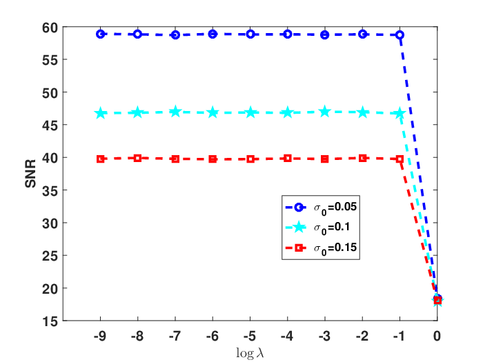
To find the better λ\lambda which derives the maximal Signal-to-Noise Ratio (SNR, 20​log⁡(‖X‖F/‖X−X^‖F)20\log(\|X\|_{F}/\|X-\hat{X}\|_{F})), a set of trails have been carried out. In Fig. 5.1 with M=750M=750, the SNR is plotted versus the regularization parameter λ\lambda for different σ0\sigma_{0} values, σ0=0.05,0.10,0.15\sigma_{0}=0.05,~0.10,~0.15, and λ\lambda is varied between 10−910^{-9} and 11, and the image evidences that the parameter λ∈[10−9,10−1]\lambda\in[10^{-9},10^{-1}] is a well selection.

Refer to caption
Fig. 5.1: Recovery performance of the constrained nuclear norm minimization (3.25) versus λ\lambda.

In order to verify the justifiability of the model (3.25), two sets of experiments have been conducted. In Fig. 5.2(a) with M=700M=700, the average relative error (‖X−X^‖F/‖X‖F\|X-\hat{X}\|_{F}/\|X\|_{F}) is plotted versus the rank rr for different standard deviation values (i.e., σ0\sigma_{0}), σ0=0.05,0.10,0.15\sigma_{0}=0.05,~0.10,~0.15, and the rank rr ranges from 44 and 88 and Fig. 5.2(b) depicts the SNR versus the number of measurements MM for different σ0\sigma_{0} values, σ0=0.05,0.10,0.15\sigma_{0}=0.05,~0.10,~0.15, and the number of measurements MM varies from 720720 to 800800 with r=6r=6. It is easy to see that as the rank of the original matrix XXdecreases and the number of measurements increases, the recovery error decreases gradually, and a decreasing standard deviation σ0\sigma_{0} leads to a better performance.

Refer to caption
Refer to caption
Fig. 5.2: (a) Relative error varying rank with M=700M=700, (b) SNR varying number of measurements with r=6r=6.

To further verify the validity of the model (3.25) recovery, we choose random Bernoulli matrix as the measurement matrix, whose entries follows Bernoulli distribution, i.e.,

Ai​j=1M​{1,p=12,−1,p=12.A_{ij}=\frac{1}{\sqrt{M}}\begin{cases}1,\quad\ \ &p=\frac{1}{2},\\ -1,\quad\ \ &p=\frac{1}{2}.\end{cases}

SNR versus the rank and the relative error versus the number of samples, the results are shown in Fig. 5.3(a) and (b) in different σ0=0.05,0.10,0.15\sigma_{0}=0.05,~0.10,~0.15. In Fig. 5.3(a), the values of the rank rr of the original matrix vary from 44 to 88 with M=700M=700 and in Fig. 5.3(b), the number of samples MM ranges from 730730 to 810810 with r=6r=6. Fig. 5.3(a) and (b) demonstrate that as the variance of noise matrix ZZ decreases, the recovery effect becomes better, and a smaller rank of the original matrix and a larger number of samples make the reconstruction error smaller (SNR larger).

Refer to caption
Refer to caption
Fig. 5.3: (a) SNR varying rank with M=700M=700, (b) Relative error varying number of samples with r=6r=6.

Finally, the effect of noise variance on the performance of model (3.25) reconstruction is illustrated by grayscale image recovery. The original image (in Fig. 5.4) has a resolution of 256×256256\times 256. The selection of measurement matrix is the same as that in Fig. 5.2. We fix the standard deviation σ=0.01\sigma=0.01 of the measurement noise ww. Due to the limitation of experimental conditions, we scale the original image to a resolution of 30×3030\times 30. The number of measurements is equal to M=2.5​r​(m+n−r)+1M=2.5r(m+n-r)+1 and the rank rr equals to 0.2​m0.2m. To access the quality of the recovered image, we adopt Structural SIMilarity (SSIM) and Peak Signal-to-Noise Ratio (PSNR). The gained results are reported in Table 5. The results show again the smaller the variance of noise, the better the recovery effect.

Refer to caption
Fig. 5.4: Grayscale image of 256×256256\times 256 pixels.
Table 5.1: PSNR||SSIM results on recovery of test image
σ0\sigma_{0} PSNR SSIM
1 0.05 35.588 0.95328
2 0.10 33.248 0.92672
3 0.15 30.142 0.86879
4 0.20 27.033 0.77871

Some experts may ask, what is the effect of the model and its associating algorithm on image denoising? We have made some attempts in this respect, but we have not yet achieved good experimental results. We are still trying to explore this issue and regard it as an important research direction in the future.

6 The proofs of theorems

Before proving our main results, we need some auxiliary lemmas.

Lemma 6.1.

(Gaussian white noise) Recall that ww is a white noise vector with 𝔼⁡(w)=0M\mathbb{E}(w)=0_{M} and Var​(w)=σ2​IM\mbox{Var}(w)=\sigma^{2}I_{M}, and that similarly ZZ is a white noise matrix satisfying 𝔼⁡(Z)=0m×n\mathbb{E}(Z)=0_{m\times n} and Var​(Z)=σ02​Im​n\mbox{Var}(Z)=\sigma^{2}_{0}I_{mn}, independent of ww. In addition, we assume that both ww and ZZ follow Gaussian distribution. Then

u=Σ1−1/2v∼ℕ(0,θIM),\displaystyle u=\Sigma^{-1/2}_{1}v\sim\mathbb{N}(0,\theta I_{M}),

where Σ1=Σ/θ\Sigma_{1}=\Sigma/\theta, Σ=σ2​IM+σ02​A​A⊤\Sigma=\sigma^{2}I_{M}+\sigma^{2}_{0}AA^{\top}, θ=σ2+m​n​σ02/M\theta=\sigma^{2}+mn\sigma^{2}_{0}/M, and v=A​vec​(Z)+wv=A\mbox{vec}(Z)+w.

Furthermore, the noise u∼ℕ⁡(0,θ​IM)u\sim\mathbb{N}(0,\theta I_{M}) satisfies

ℙ⁡(‖u‖2≤θ⁡(M+2​M​log⁡M))≥1−1M,\displaystyle\mathbb{P}\left(\|u\|_{2}\leq\sqrt{\theta(M+2\sqrt{M\log M})}\right)\geq 1-\frac{1}{M}, (6.32)
{ℙ(∥u∥p≤M1/pθ⁡(1+2​M−1​log⁡M))>1−1M,0≤p<2,ℙ(∥u∥p≤θ⁡(M+2​M​log⁡M))≥1−1M,p≥2.\displaystyle\begin{cases}\mathbb{P}\left(\|u\|_{p}\leq M^{1/p}\sqrt{\theta(1+2\sqrt{M^{-1}\log M})}\right)>1-\frac{1}{M},~0\leq p<2,\\ \mathbb{P}\left(\|u\|_{p}\leq\sqrt{\theta(M+2\sqrt{M\log M})}\right)\geq 1-\frac{1}{M},~p\geq 2.\end{cases} (6.33)
Proof of the lemma 6.1.

Note that AA is a linear transformation. By applying the property of Gaussian random vector, the definition of covariance matrix and some elementary calculations, we get

v∼ℕ⁡(0,σ2​IM+σ02​A​A⊤).\displaystyle v\sim\mathbb{N}(0,\sigma^{2}I_{M}+\sigma^{2}_{0}AA^{\top}).

Since Σ−1/21\Sigma^{-1/2}_{1} is a linear map, we get

u=Σ1−1/2v∼ℕ(0,θIM).\displaystyle u=\Sigma^{-1/2}_{1}v\sim\mathbb{N}(0,\theta I_{M}).

The proof of the inequality (6.32) is similar to Lemma I​I​I​.3III.3 in [20].

In the following, we prove the equation (6.33). Since the proofs of two cases are similar, we only provide the proof of 0≤p<20\leq p<2. By employing the inequality that ‖x‖2≤‖x‖p≤M1/p−1/2​‖x‖2\|x\|_{2}\leq\|x\|_{p}\leq M^{1/p-1/2}\|x\|_{2} for all x∈ℝMx\in\mathbb{R}^{M} and fixed 1≤p<21\leq p<2 and ‖u‖2≤θ⁡(M+2​M​log⁡M)\|u\|_{2}\leq\sqrt{\theta(M+2\sqrt{M\log M})}, we get

‖u‖p≤M1/p−1/2​θ⁡(M+2​M​log⁡M),\|u\|_{p}\leq M^{1/p-1/2}\sqrt{\theta(M+2\sqrt{M\log M})},

which implies

ℙ⁡(‖u‖p≤M1/p​θ⁡(1+2​M−1​log⁡M))>ℙ⁡(‖u‖2≤θ⁡(M+2​M​log⁡M))≥1−1M.\displaystyle\mathbb{P}\left(\|u\|_{p}\leq M^{1/p}\sqrt{\theta(1+2\sqrt{M^{-1}\log M})}\right)>\mathbb{P}\left(\|u\|_{2}\leq\sqrt{\theta(M+2\sqrt{M\log M})}\right)\geq 1-\frac{1}{M}.

∎

Lemma 6.2.

(Gaussian mixture noise) Assume that i.i.d. wiw_{i} and Zi​jZ_{ij} follow respectively two-term Gaussian mixture models, i.e., wi∼(1−ξ)ℕ(0,σ2)+ξℕ(0,κσ2),i=1,⋯,Mw_{i}\sim(1-\xi)\mathbb{N}(0,\sigma^{2})+\xi\mathbb{N}(0,\kappa\sigma^{2}),~i=1,\cdots,M, and Zi​j∼(1−η)ℕ(0,σ02)+ηℕ(0,γσ02),i=1,⋯,m,j=1,⋯,nZ_{ij}\sim(1-\eta)\mathbb{N}(0,\sigma^{2}_{0})+\eta\mathbb{N}(0,\gamma\sigma^{2}_{0}),~i=1,\cdots,m,~j=1,\cdots,n, where 0≤ξ<1​(0≤η<1)0\leq\xi<1~(0\leq\eta<1) represents the portion of outliers in the noise and κ>1​(γ>1)\kappa>1~(\gamma>1) stands for the strength of outliers. Then

u=Σ1′−1/2v∼ℕ(0,θ′IM),\displaystyle u=\Sigma^{\prime-1/2}_{1}v\sim\mathbb{N}(0,\theta^{\prime}I_{M}),

namely, uiu_{i} obeys the Gaussian mixture noise, i.e., ui∼(1−ξ)​ℕ​(0,σ2)+ξ​ℕ​(0,κ​σ2)+(1−η)​ℕ​(0,m​n​σ02/M)+η​ℕ​(0,m​n​γ​σ02/M)u_{i}\sim(1-\xi)\mathbb{N}(0,\sigma^{2})+\xi\mathbb{N}(0,\kappa\sigma^{2})+(1-\eta)\mathbb{N}(0,mn\sigma^{2}_{0}/M)+\eta\mathbb{N}(0,mn\gamma\sigma^{2}_{0}/M), where Σ1′=Σ′/θ′\Sigma^{\prime}_{1}=\Sigma^{\prime}/\theta^{\prime}, Σ′=[(1−ξ)+κ​ξ]​σ2​IM+[(1−η)+γ​η]​σ02​A​A⊤\Sigma^{\prime}=[(1-\xi)+\kappa\xi]\sigma^{2}I_{M}+[(1-\eta)+\gamma\eta]\sigma^{2}_{0}AA^{\top}, θ′=[(1−ξ)+κ​ξ]​σ2+m​n​[(1−η)+γ​η]​σ02/M\theta^{\prime}=[(1-\xi)+\kappa\xi]\sigma^{2}+mn[(1-\eta)+\gamma\eta]\sigma^{2}_{0}/M, and v=A​vec​(Z)+wv=A\mbox{vec}(Z)+w.

Besides, the noise u∼ℕ⁡(0,θ′​IM)u\sim\mathbb{N}(0,\theta^{\prime}I_{M}) fulfills

{ℙ(∥u∥p≤M1/pθ′​(1+2​M−1​log⁡M))>1−1M,0≤p<2,ℙ(∥u∥p≤θ′​(M+2​M​log⁡M))≥1−1M,p≥2,\displaystyle\begin{cases}\mathbb{P}\left(\|u\|_{p}\leq M^{1/p}\sqrt{\theta^{\prime}(1+2\sqrt{M^{-1}\log M})}\right)>1-\frac{1}{M},~0\leq p<2,\\ \mathbb{P}\left(\|u\|_{p}\leq\sqrt{\theta^{\prime}(M+2\sqrt{M\log M})}\right)\geq 1-\frac{1}{M},~p\geq 2,\end{cases} (6.34)

where θ′=[(1−ξ)+κ​ξ]​σ2+m​n​[(1−η)+γ​η]​σ02/M\theta^{\prime}=[(1-\xi)+\kappa\xi]\sigma^{2}+mn[(1-\eta)+\gamma\eta]\sigma^{2}_{0}/M. And similar to [21], the pp-th moment of such a noise process is given by

𝔼⁡{‖u‖pp}=M​2p/2​θ′p/2​Γ​(p+12)π\displaystyle\mathbb{E}\{\|u\|_{p}^{p}\}=\frac{M2^{p/2}\theta^{\prime p/2}\Gamma(\frac{p+1}{2})}{\sqrt{\pi}} (6.35)

where θ′=[(1−ξ)+κ​ξ]​σ2+m​n​[(1−η)+γ​η]​σ02/M\theta^{\prime}=[(1-\xi)+\kappa\xi]\sigma^{2}+mn[(1-\eta)+\gamma\eta]\sigma^{2}_{0}/M.

The following lemma presents a matrix of Stechkin’s bound generalizing the result of sparse vectors [24] to the case of low-rank matrices.

Lemma 6.3.

([22]) Let X∈ℝm×nX\in\mathbb{R}^{m\times n} and r≤min⁡{m,n}r\leq\min\{m,n\}. Then, for p>0p>0,

‖X[r]c‖p≤1r1−1/p​‖X‖∗.\displaystyle\|X_{[r]^{c}}\|_{p}\leq\frac{1}{r^{1-1/p}}\|X\|_{*}.

The following lemma is a useful inequality on matrix norm.

Lemma 6.4.

([23]) For any X,Y∈ℝm×nX,Y\in\mathbb{R}^{m\times n}, we have

‖X−Y‖∗≥∑i=1n0|σi​(X)−σi​(Y)|,\displaystyle\|X-Y\|_{*}\geq\sum^{n_{0}}_{i=1}|\sigma_{i}(X)-\sigma_{i}(Y)|,

where n0=min⁡{m,n}n_{0}=\min\{m,n\}.

The result below reveals that the distance between the original matrix and its corresponding solution is bounded by the best rr-rank approximation error and the Euclidean norm of the difference between their measurements provided that the Frobenius-robust rank null space property.

Lemma 6.5.

Set δ1=δ/(1−δ)\delta_{1}=\delta/(1-\delta) with δ<1/2\delta<1/2. Assume that 𝒜:ℝm×n→ℝM\mathcal{A}:\mathbb{R}^{m\times n}\to\mathbb{R}^{M} fulfills the Frobenius-robust rank null space property with constants 0<ρ<10<\rho<1 and τ>0\tau>0. Then, a solution X∗X^{*} of problem (3.25) approximates the matrix XX with errors

‖X−X∗‖∗≤2​(1+ρ)1−ρ​‖X[r]c‖∗+2​τ​r(1−ρ)​1−δ1​‖ℬ⁡(X−X∗)‖2.\displaystyle\|X-X^{*}\|_{*}\leq\frac{2(1+\rho)}{1-\rho}\|X_{[r]^{c}}\|_{*}+\frac{2\tau\sqrt{r}}{(1-\rho)\sqrt{1-\delta_{1}}}\|\mathcal{B}(X-X^{*})\|_{2}. (6.36)
Proof of the lemma 6.5.

By exploiting Lemma 6.4, we get

‖X∗‖∗\displaystyle\|X^{*}\|_{*} =‖X−(X−X∗)‖∗≥∑i=1n0|σi​(X)−σi​(X−X∗)|\displaystyle=\|X-(X-X^{*})\|_{*}\geq\sum^{n_{0}}_{i=1}|\sigma_{i}(X)-\sigma_{i}(X-X^{*})|
=∑i=1r|σi​(X)−σi​(X−X∗)|+∑i=r+1n0|σi​(X)−σi​(X−X∗)|\displaystyle=\sum^{r}_{i=1}|\sigma_{i}(X)-\sigma_{i}(X-X^{*})|+\sum^{n_{0}}_{i=r+1}|\sigma_{i}(X)-\sigma_{i}(X-X^{*})|
≥∑i=1r(σi​(X)−σi​(X−X∗))+∑i=r+1n0(σi​(X−X∗)−σi​(X)).\displaystyle\geq\sum^{r}_{i=1}(\sigma_{i}(X)-\sigma_{i}(X-X^{*}))+\sum^{n_{0}}_{i=r+1}(\sigma_{i}(X-X^{*})-\sigma_{i}(X)).

Therefore,

‖(X−X∗)[r]c‖∗\displaystyle\|(X-X^{*})_{[r]^{c}}\|_{*} ≤‖X∗‖∗−∑i=1rσi​(X)+∑i=1rσi​(X−X∗)+∑i=r+1n0σi​(X)\displaystyle\leq\|X^{*}\|_{*}-\sum^{r}_{i=1}\sigma_{i}(X)+\sum^{r}_{i=1}\sigma_{i}(X-X^{*})+\sum^{n_{0}}_{i=r+1}\sigma_{i}(X)
≤(a)​‖X∗‖∗−‖X‖∗+r​‖(X−X∗)[r]‖F+2​‖X[r]c‖∗\displaystyle\overset{\text{(a)}}{\leq}\|X^{*}\|_{*}-\|X\|_{*}+\sqrt{r}\|(X-X^{*})_{[r]}\|_{F}+2\|X_{[r]^{c}}\|_{*}
≤(b)​r​‖(X−X∗)[r]‖F+2​‖X[r]c‖∗,\displaystyle\overset{\text{(b)}}{\leq}\sqrt{r}\|(X-X^{*})_{[r]}\|_{F}+2\|X_{[r]^{c}}\|_{*},

where (a) follows from Ho¨\ddot{o}lder’s inequality, and (b) is due to the minimality of X∗X^{*}. Employing the Frobenius-robust rank null space property of the linear measurement map ℬ\mathcal{B} to the inequality above, rearranging the terms and observing 0<ρ<10<\rho<1, we get

‖(X−X∗)[r]c‖∗≤11−ρ​(τ​r1−δ1​‖ℬ⁡(X−X∗)‖2+2​‖X[r]c‖∗).\displaystyle\|(X-X^{*})_{[r]^{c}}\|_{*}\leq\frac{1}{1-\rho}\left(\frac{\tau\sqrt{r}}{\sqrt{1-\delta_{1}}}\|\mathcal{B}(X-X^{*})\|_{2}+2\|X_{[r]^{c}}\|_{*}\right). (6.37)

Then,

‖X−X∗‖∗\displaystyle\|X-X^{*}\|_{*} =‖(X−X∗)[r]‖∗+‖(X−X∗)[r]c‖∗\displaystyle=\|(X-X^{*})_{[r]}\|_{*}+\|(X-X^{*})_{[r]^{c}}\|_{*}
≤(a)​r​‖(X−X∗)[r]‖F+‖(X−X∗)[r]c‖∗\displaystyle\overset{\text{(a)}}{\leq}\sqrt{r}\|(X-X^{*})_{[r]}\|_{F}+\|(X-X^{*})_{[r]^{c}}\|_{*}
≤(b)​(1+ρ)​‖(X−X∗)[r]c‖∗+τ​r1−δ1​‖ℬ⁡(X−X∗)‖2\displaystyle\overset{\text{(b)}}{\leq}(1+\rho)\|(X-X^{*})_{[r]^{c}}\|_{*}+\frac{\tau\sqrt{r}}{\sqrt{1-\delta_{1}}}\|\mathcal{B}(X-X^{*})\|_{2}
≤(c)​2​(1+ρ)1−ρ​‖X[r]c‖∗+2​τ​r(1−ρ)​1−δ1​‖ℬ⁡(X−X∗)‖2,\displaystyle\overset{\text{(c)}}{\leq}\frac{2(1+\rho)}{1-\rho}\|X_{[r]^{c}}\|_{*}+\frac{2\tau\sqrt{r}}{(1-\rho)\sqrt{1-\delta_{1}}}\|\mathcal{B}(X-X^{*})\|_{2},

where (a) is from Ho¨\ddot{o}lder’s inequality, (b) is due to the Frobenius-robust rank null space property of ℬ\mathcal{B}, and (c) follows from the inequality (6.37). The proof is complete. ∎

Proof of the theorem 3.3.

By utilizing Lemma 6.3, we get

‖X−X∗‖F\displaystyle\|X-X^{*}\|_{F} ≤(a)​‖(X−X∗)[r]‖F+‖(X−X∗)[r]c‖F\displaystyle\overset{\text{(a)}}{\leq}\|(X-X^{*})_{[r]}\|_{F}+\|(X-X^{*})_{[r]^{c}}\|_{F}
≤‖(X−X∗)[r]‖F+1r​‖X−X∗‖∗\displaystyle\leq\|(X-X^{*})_{[r]}\|_{F}+\frac{1}{\sqrt{r}}\|X-X^{*}\|_{*}
≤(b)​1+ρr​‖X−X∗‖∗+τ1−δ1​‖ℬ⁡(X−X∗)‖2,\displaystyle\overset{\text{(b)}}{\leq}\frac{1+\rho}{\sqrt{r}}\|X-X^{*}\|_{*}+\frac{\tau}{\sqrt{1-\delta_{1}}}\|\mathcal{B}(X-X^{*})\|_{2},

where for (a) we make use of the triangular inequality, and (b) follows from the Frobenius-robust rank null space property of ℬ\mathcal{B}. Plugging (6.36) into the above inequality, observing the fact that ‖u‖2≤ϵ\|u\|_{2}\leq\epsilon, and due to the inequality ‖ℬ⁡(X−X∗)‖2≤‖ℬ⁡(X)−y~‖2+‖ℬ⁡(X∗)−y~‖2\|\mathcal{B}(X-X^{*})\|_{2}\leq\|\mathcal{B}(X)-\tilde{y}\|_{2}+\|\mathcal{B}(X^{*})-\tilde{y}\|_{2}, the result is deduced. ∎

The following outcome clears that under the stable rank null space property, the distance between the matrix to be recovered and its associating solution is controlled by the best rr-rank approximation error and the Euclidean distance between their measurements.

Lemma 6.6.

Set δ1=δ/(1−δ)\delta_{1}=\delta/(1-\delta) with δ<1/2\delta<1/2. Let X∗X^{*} be the optimal solution of problem (3.25) with ‖ℬ⁡(X∗)−y~‖2≤ϵ\|\mathcal{B}(X^{*})-\tilde{y}\|_{2}\leq\epsilon. Suppose that we observe y~=ℬ⁡(X)+u\tilde{y}=\mathcal{B}(X)+u with ‖ℬ⁡(X)−y~‖2≤ϵ\|\mathcal{B}(X)-\tilde{y}\|_{2}\leq\epsilon and 𝒜:ℝm×n→ℝM\mathcal{A}:\mathbb{R}^{m\times n}\to\mathbb{R}^{M} meets the stable rank null space property with constants 0<ρ<10<\rho<1 and τ>0\tau>0. Then,

‖X−X∗‖∗≤2​(1+ρ)1−ρ​‖X[r]c‖∗+2​τ(1−ρ)​1−δ1​‖ℬ⁡(X−X∗)‖2.\displaystyle\|X-X^{*}\|_{*}\leq\frac{2(1+\rho)}{1-\rho}\|X_{[r]^{c}}\|_{*}+\frac{2\tau}{(1-\rho)\sqrt{1-\delta_{1}}}\|\mathcal{B}(X-X^{*})\|_{2}. (6.38)
Proof of the lemma 6.6.

The proof is similar to that of Lemma 6.5. ∎

Proof of the theorem 3.10.

Combining with the stable rank null space property, Cauchy-Schwarz inequality, Lemmas 6.3 and 6.6, the desired result is established. This completes the proof. ∎

7 Conclusion

Although the literature on low-rank matrix recovery is almost silent on the impact of pre-measurement noise on recovery performance, this paper certificated that it maybe have an important effect on signal-noise-ratio. Certainly, we indicated that for the widespread measuring formula employed in low-rank matrix recovery, the model with pre-measurement noise is, after whitening, equivalent to a standard model with merely additional noise and a raise in the noise variance by a factor of m​n/Mmn/M. We presented bounds on the RIP constants and the SSR constants of new linear measurement map which cleared that as m,n,M→∞m,~n,~M\to\infty with m​n/M→0mn/M\to 0, the RIP constants are fundamentally unaltered. As the performance of standard reconstruction approaches is regularly expressed with respect to the RIP constants, this demonstrates that, these approaches manipulate like the standard, as well as noise folding causes a large noise increase. Besides, based on the two kinds of null space properties, we extended the study to the noise folding scenario, established sufficient conditions for robustly reconstructing low-rank matrix itself subject to noise, and provided upper bound estimations of recovery error. Furthermore, the minimal number of measurement such that sufficient condition based on FRRNSP obeys was gained. Numerical simulations are presented to verify the theoretical results.

8 Acknowledgments

This work was supported by Natural Science Foundation of China (Nos. 61673015, 61273020), Fundamental Research Funds for the Central Universities (Nos. XDJK2015A007, XDJK2018C076, SWU1809002), Youth Science and technology talent development project (No. Qian jiao he KY zi [2018]313), Science and technology Foundation of Guizhou province (No. Qian ke he Ji Chu [2016]1161), Guizhou province natural science foundation in China (No. Qian Jiao He KY [2016]255).

References

  • [1] J. Abernethy, F. Bach, T. Evgeniou, and J. P. Vert, ¡°A new approach to collaborative filtering: Operator estimation with spectral regularization,¡± J. Mach. Learn. Res., vol. 10, pp. 803¨C826, Mar. 2009.
  • [2] Chang, X., Zhong, Y., Wang, Y., & Lin, S. (2018). Unified Low-Rank Matrix Estimate via Penalized Matrix Least Squares Approximation. IEEE transactions on neural networks and learning systems, (99), 1-12.
  • [3] Lin J, Li S. Convergence of projected Landweber iteration for matrix rank minimization. Appl Comput Harmon Anal, 2014, 36: 316-325
  • [4] Xu, L., Lin, S., Zeng, J., Liu, X., Fang, Y., & Xu, Z. (2018). Greedy criterion in orthogonal greedy learning. IEEE transactions on cybernetics, 48(3), 955-966.
  • [5] Recht B, Fazel M, Parrilo P A. Guaranteed minimum rank solutions of linear matrix equations via nuclear norm minimization. SIAM Rev, 2010, 52: 471-501
  • [6] R. Mazumder, T. Hastie, and R. Tibshirani, ¡°Spectral regularization algorithms for learning large incomplete matrices,¡± J. Mach. Learn. Res., vol. 11, pp. 2287-2322, 2010.
  • [7] Y. Wang, L. Lin, Q. Zhao, T. Yue, D. Meng, and Y. Leung, ¡°Compressive sensing of hyperspectral images via joint tensor tucker decomposition and weighted total variation regularization,¡± IEEE Geosci. Remote Sens. Lett., vol. 14, no. 12, pp. 2457-2461, Dec. 2017.
  • [8] E. J. Cande`\grave{e}s, X. Li, Y. Ma, and J. Wright. Robust principal component analysis? J. ACM, 58(1):1¨C37, 2009.
  • [9] Waters, A. E., Sankaranarayanan, A. C., & Baraniuk, R. (2011). SpaRCS: Recovering low-rank and sparse matrices from compressive measurements. In Advances in neural information processing systems (pp. 1089-1097).
  • [10] A. Chakrabarti and T. Zickler. Statistics of Real-World Hyperspectral Images. In IEEE Int. Conf. Comp. Vis., Colorado Springs, CO, June 2011.
  • [11] Chen, Y., Xu, H., Caramanis, C., & Sanghavi, S. (2011). Robust matrix completion and corrupted columns. In Proceedings of the 28th International Conference on Machine Learning (ICML-11) (pp. 873-880).
  • [12] Arias-Castro, E., & Eldar, Y. C. (2011). Noise folding in compressed sensing. IEEE Signal Processing Letters, 18(8), 478-481.
  • [13] Peter, S., Artina, M., & Fornasier, M. (2015). Damping noise-folding and enhanced support recovery in compressed sensing. IEEE Transactions on Signal Processing, 63(22), 5990-6002.
  • [14] E. J. Cande`\grave{e}s, J. Romberg, and T. Tao, ¡°Robust uncertainty principles: Exact signal reconstruction fromhighly incomplete frequency information,¡± IEEE Trans. Inf. Theory, vol. 52, no. 2, pp. 489-509, Feb. 2006.
  • [15] D. L. Donoho, ¡°Compressed sensing,¡± IEEE Trans. Inf. Theory, vol. 52, no. 4, pp. 1289-1306, 2006.
  • [16] L. C. Kong and N. H. Xiu, “Exact low-rank matrix recovery via nonconvex Schatten pp-minimization,” Asia Pac. J. Oper. Res., vol. 30, no. 3, pp. 1340010, Jun. 2013.
  • [17] R. Zhang and S. Li, “Optimal RIP Bounds for Sparse Signals Recovery via lpl_{p} Minimization,” Appl. Comput. Harmon. Anal., 2018, doi: org/10.1016/j.acha.2017.10.004.
  • [18] W. G. Chen and Y. L. Li, “Stable recovery of low-rank matrix via nonconvex Schatten pp-minimization,” Sci. China Math., vol. 58, no. 12, pp 2643-2654, Dec. 2015.
  • [19] Vershynin, R. (2010). Introduction to the non-asymptotic analysis of random matrices. arXiv preprint arXiv:1011.3027.
  • [20] Lin J, Li S, Shen Y. New bounds for restricted isometry constants with coherent tight frames[J]. IEEE Transactions on Signal Processing, 2013, 61(3): 611-621.
  • [21] Wen F, Liu P, Liu Y, et al. Robust Sparse Recovery in Impulsive Noise via ℓp\ell_{p}-ℓ1\ell_{1} Optimization[J]. IEEE Transactions on Signal Processing, 2017, 65(1): 105-118.
  • [22] Kabanava, M., Kueng, R., Rauhut, H., & Terstiege, U. (2016). Stable low-rank matrix recovery via null space properties. Information and Inference: A Journal of the IMA, 5(4), 405-441.
  • [23] Horn, R. & Johnson, C. Topics in Matrix Analysis. Cambridge: Cambridge University Press, 1991.
  • [24] Foucart, S. & Rauhut, H. (2013) A mathematical introduction to compressive sensing. Applied and Numerical Harmonic Analysis (J. S. Benedetto ed.). New York: Birkh¡§auser/Springer, 2013.
  • [25] Canyi Lu, Jiashi Feng, Shuicheng Yan, and Zhouchen Lin. A unified alternating direction method of multipliers by majorization minimization. TPAMI, 40(3):527¨C541, 2018.
  • [26] Lu C, Feng J, Lin Z, et al. Exact low tubal rank tensor recovery from gaussian measurements[J]. arXiv preprint arXiv:1806.02511, 2018.
  • [27] Feng Q, Wang J, Zhang F. Block-sparse signal recovery based on truncated ℓ1\ell_{1} minimisation in non-Gaussian noise[J]. IET Communications, 2019, 13(2): 251-258.