跳到论文正文
W Papers独立论文阅读器 arXiv:2003.03070 论文正文 计算阅读时间 · 0%
引用这篇论文根据当前论文元数据生成,正式投稿前建议核对。


License: arXiv.org perpetual non-exclusive license
arXiv:2003.03070v1 [math.PR] 06 Mar 2020
\online\ensubject

fdsfd

\ArticleType

ARTICLES\Year2017 \MonthJanuary\Vol60 \No1 \BeginPage1 \DOI10.1007/s11425-000-0000-0 \ReceiveDateJanuary 1, 2017 \AcceptDateJanuary 1, 2017

The Graph Limit of The Minimizer of The Onsager-Machlup Functional and Its Computation

qd2125@columbia.edu tieli@pku.edu.cn lixiaoguang@hunnu.edu.cn matrw@nus.edu.sg

\MSC

14Axx, 32Bxx

The Graph Limit of The Minimizer of The Onsager-Machlup Functional and Its Computation

Qiang Du    Tiejun Li    Xiaoguang Li    Weiqing Ren Address: Department of Applied Physics and Applied Mathematics, Columbia University, New York, NY 10027, USA Address: LMAM and School of Mathematical Sciences, Peking University, Beijing 100871, P.R.China Address: Beijing Computational Science Research Center, Beijing, 100193, China,
MOE-LCSM, School of Mathematics and Statistics, Hunan Normal University, Changsha, Hunan 410081 , P. R. China
Address: Department of Mathematics, National University of Singapore, Singapore 119076, Singapore
Abstract

The Onsager-Machlup (OM) functional is well-known for characterizing the most probable transition path of a diffusion process with non-vanishing noise. However, it suffers from a notorious issue that the functional is unbounded below when the specified transition time TT goes to infinity. This hinders the interpretation of the results obtained by minimizing the OM functional. We provide a new perspective on this issue. Under mild conditions, we show that although the infimum of the OM functional becomes unbounded when TT goes to infinity, the sequence of minimizers does contain convergent subsequences on the space of curves. The graph limit of this minimizing subsequence is an extremal of the abbreviated action functional, which is related to the OM functional via the Maupertuis principle with an optimal energy. We further propose an energy-climbing geometric minimization algorithm (EGMA) which identifies the optimal energy and the graph limit of the transition path simultaneously. This algorithm is successfully applied to several typical examples in rare event studies. Some interesting comparisons with the Freidlin-Wentzell action functional are also made.

keywords
Onsager-Machlup functional, Freidlin-Wentzell functional, graph limit, geometric minimization, Maupertuis principle

1 Introduction

Consider a stochastic dynamics modeled by the stochastic differential equation (SDE)

d​𝑿t=𝒃⁡(𝑿t)​d​t+2​ε​d​𝑾t,\,\mathrm{d}\bm{X}_{t}=\bm{b}(\bm{X}_{t})\,\mathrm{d}t+\sqrt{2\varepsilon}\,\mathrm{d}\bm{W}_{t}, (1)

where 𝑿t,𝒃∈ℝd\bm{X}_{t},\bm{b}\in\mathbb{R}^{d}, 𝑾t=(Wt1,Wt2,…,Wtd)\bm{W}_{t}=(W^{1}_{t},W^{2}_{t},\ldots,W^{d}_{t}) is the standard dd-dimensional Wiener process with 𝔼​Wti=0\mathbb{E}W^{i}_{t}=0 and 𝔼⁡(Wti​Wsj)=δi​j⋅min⁡(t,s)\mathbb{E}(W^{i}_{t}W^{j}_{s})=\delta_{ij}\cdot\min(t,s) for i,j=1,…,di,j=1,\ldots,d and t,s∈ℝ+t,s\in\mathbb{R}^{+}. Due to the presence of the noise, the system makes transitions from one metastable state to another; when ε\varepsilon is small, however, these transitions happen on a time scale which is much longer than the relaxation time scale of the system. These rare but important transition events are very common in different fields of science, and their study has attracted much attention in recent years [2, 3, 4, 14, 21, 32]. One major object in the study of such rare events is to understand the transition mechanism, which can be characterized by the most probable path (MPP), i.e. the transition path with a dominant probability, connecting an initial state 𝒙s\bm{x}_{s} and a terminal state 𝒙f\bm{x}_{f} in the configuration space. How to characterize and compute these transition paths is a fundamental problem in the study of rare events [9, 10, 13, 22, 30, 40, 34, 37] and also the focus of this paper. In particular, we study the transition path at finite noise provided by the Onsager-Machlup functional and its graph limit as the prescribed transition time goes to infinity.

In the zero noise limit, i.e. ε→0\varepsilon\to 0, it is well-known from the large deviation theory that the MPP from 𝒙s\bm{x}_{s} to 𝒙f\bm{x}_{f} is given by the solution to the double minimization problem [11, 22]

SFW​(𝒙s,𝒙f)=infT>0infψ⁡(0)=𝒙s,ψ⁡(T)=𝒙fSTFW​[ψ],S^{{\rm FW}}(\bm{x}_{s},\bm{x}_{f})=\inf\limits_{T>0}\inf\limits_{\psi(0)=\bm{x}_{s},\psi(T)=\bm{x}_{f}}S_{T}^{{\rm FW}}[\psi], (2)

where ψ⁡(t)\psi(t) is an absolutely continuous function on [0,T][0,T] and STFW​[ψ]S_{T}^{{\rm FW}}[\psi] is the Freidlin-Wentzell (FW) action functional

STFW​[ψ]=∫0T12​|ψ˙−𝒃⁡(ψ)|2​𝑑t.S_{T}^{{\rm FW}}[\psi]=\int_{0}^{T}\frac{1}{2}|\dot{\psi}-\bm{b}(\psi)|^{2}\,\mathrm{d}t. (3)

Here ψ˙\dot{\psi} denotes the time derivative of ψ\psi. It is known that the infimum is achieved when T=∞T=\infty if the MPP connecting 𝒙s\bm{x}_{s} and 𝒙f\bm{x}_{f} passes through a stationary point of the deterministic dynamics 𝒙˙=𝒃⁡(𝒙)\dot{\bm{x}}=\bm{b}(\bm{x}). The quasi-potential SFW​(𝒙s,𝒙f)=infTinfψSTFW​[ψ]S^{{\rm FW}}(\bm{x}_{s},\bm{x}_{f})=\inf_{T}\inf_{\psi}S_{T}^{{\rm FW}}[\psi] characterizes, in the zero-noise limit, the transition rate, the invariant distribution of the stochastic dynamics and so forth. To avoid the difficulty caused by the infinite transition time, an alternative approach, which uses the arclength parameterization, has been proposed for the computation of the MPP on the space of curves [22].

For finite ε>0\varepsilon>0, the Onsager-Machlup (OM) functional has been proposed in the literature to find the MPP [8, 16, 17, 25, 30, 35]. The OM functional is given by

STOM​[ψ]=∫0TL⁡(ψ,ψ˙)​𝑑tS_{T}^{{\rm OM}}[\psi]=\int_{0}^{T}L(\psi,\dot{\psi})\,\mathrm{d}t (4)

if ψ\psi is absolutely continuous on [0,T][0,T], and takes the infinite value otherwise. Here the OM Lagrangian is given by

L(𝒙,𝒚)=12|𝒚−𝒃(𝒙)|2+ε∇⋅𝒃(𝒙)=12|𝒚|2−𝒃(𝒙)⋅𝒚−U(𝒙),L(\bm{x},\bm{y})=\frac{1}{2}\left|\bm{y}-\bm{b}(\bm{x})\right|^{2}+\varepsilon\nabla\cdot\bm{b}(\bm{x})=\frac{1}{2}\left|\bm{y}\right|^{2}-\bm{b}(\bm{x})\cdot\bm{y}-U(\bm{x}), (5)

where U⁡(x)U(x), the so-called path potential [30], is given by

U(𝒙)=−ε∇⋅𝒃(𝒙)−12|𝒃(𝒙)|2.U(\bm{x})=-\varepsilon\nabla\cdot\bm{b}(\bm{x})-\frac{1}{2}\left|\bm{b}(\bm{x})\right|^{2}. (6)

The OM functional was first introduced by Onsager and Machlup for SDEs with linear drift 𝒃⁡(𝒙)=−γ​𝒙\bm{b}(\bm{x})=-\gamma\bm{x} and constant diffusion by means of path integrals [29]. Indeed, their original formulation does not contain the term ε∇⋅𝒃(𝒙)\varepsilon\nabla\cdot\bm{b}(\bm{x}) in (5) as this is only a constant in the case of linear drift. It was later generalized to cases with nonlinear drift and non-constant diffusion terms based on either physical arguments [20] or more rigorous mathematical derivations [18, 23, 33, 36]. It was also argued in [9] that, in the scalar case with a constant diffusion, the MPP is given by the minimizer of the OM functional. Indeed, as shown in [18, 23, 33], the OM functional arises from the limiting probability of a δ\delta-ball problem, i.e.

ℙ⁡(sup0≤t≤T|𝑿t−ψ⁡(t)|≤δ)∼C​exp⁡(−2​ε​λ​Tδ2)​exp⁡(−12​ε​STOM​[ψ])\mathbb{P}\left(\sup_{0\leq t\leq T}|\bm{X}_{t}-\psi(t)|\leq\delta\right)\sim C\exp\left(-\frac{2\varepsilon\lambda T}{\delta^{2}}\right)\exp\left(-\frac{1}{2\varepsilon}S^{{\rm OM}}_{T}[\psi]\right) (7)

as δ→0+\delta\rightarrow 0+. Here ε>0\varepsilon>0 is fixed, CC is a positive constant and λ\lambda is the leading eigenvalue of the operator −12​Δ-\frac{1}{2}\Delta with zero boundary condition on the domain |𝒙|≤1|\bm{x}|\leq 1. The first exponential term on the right hand side of (7) can be also identified as the probability ℙ⁡(sup0≤t≤T|2​ε​𝑾t|≤δ)\mathbb{P}(\sup_{0\leq t\leq T}|\sqrt{2\varepsilon}\bm{W}_{t}|\leq\delta). Equation (7) shows that the minimizer of the OM functional characterizes the MPP under a suitable rescaling as δ→0\delta\rightarrow 0 while ε>0\varepsilon>0 is fixed. This methodology has been used to find the MPP in many practical problems, such as in the study of transition pathways of phage-λ\lambda switching [35], conformation changes of polymer systems [16, 17], protein folding pathways [25], and the maximum posteriori estimator [8], etc.

Although both the FW and OM functionals are widely used in applications, the connection between them is not fully understood. In practice, making the choice between the FW and OM functionals is often still a dilemma. The minimization of the two functionals gives different results and the minimizer of the OM functional is even dependent on the choice of the transition time TT. Understanding the relations between the FW and OM functionals is thus an interesting mathematical problem. One formal connection between these two is that the FW functional can be obtained from the OM functional by simply setting ε=0\varepsilon=0, therefore, they are likely equivalent in the zero-noise limit under certain conditions. Another formal connection can be made via the path integral approach. With the Girsanov theorem, we have

𝔼F[𝑿t]=𝔼(F[𝑾t]exp(−12∫0T|𝒃(𝑾t)|2dt+∫0T𝒃(𝑾t)d𝑾t))\mathbb{E}F[\bm{X}_{t}]=\mathbb{E}\Big(F[\bm{W}_{t}]\exp\big(-\frac{1}{2}\int_{0}^{T}|\bm{b}(\bm{W}_{t})|^{2}\,\mathrm{d}t+\int_{0}^{T}\bm{b}(\bm{W}_{t})\,\mathrm{d}\bm{W}_{t}\big)\Big) (8)

for Brownian functional F⁡[𝑿]F[\bm{X}], where we take ε=1/2\varepsilon=1/2 for simplicity and 𝑿t\bm{X}_{t} is the solution of the SDE (1). In the path integral, we formally represent the Wiener measure using the density p(𝒙)=Z−1exp(−12∫0T|𝒙˙|2dt)p(\bm{x})=Z^{-1}\exp\big(-\frac{1}{2}\int_{0}^{T}|\dot{\bm{x}}|^{2}\,\mathrm{d}t\big). Then the path weight for {𝑿t}t∈[0,T]\{\bm{X}_{t}\}_{t\in[0,T]} will be given by the exponential of the FW or OM functional respectively, depending on whether Ito or Stratonovich version of the stochastic integral ∫0T𝒃⁡(𝑾t)​d​𝑾t\int_{0}^{T}\bm{b}(\bm{W}_{t})\,\mathrm{d}\bm{W}_{t} being interpreted as ∫0T𝒃⁡(𝒙)⋅𝒙˙​𝑑t\int_{0}^{T}\bm{b}(\bm{x})\cdot\dot{\bm{x}}\,\mathrm{d}t in path integrals. There have been some investigations on the relationship between the FW and OM functionals. For example, in [31] it was shown that the OM functional Γ\Gamma-converges to a functional completely characterized by the FW functional when T=ε−1T=\varepsilon^{-1} and ε→0\varepsilon\rightarrow 0; in [30], the numerical studies showed that in general the OM functional does not have a lower bound as T→∞T\rightarrow\infty, and the minimizer of the OM functional with ε>0\varepsilon>0 exhibits quite different behavior compared to that of the FW functional.

Accepting the assertion that the minimizer of OM functional characterizes the MPP for the SDEs (1) when ε\varepsilon is finite, in this paper, we analyze the behaviour of the minimizer as the prescribed transition time TT goes to infinity. This is meaningful since the transition time between metastable states is usually exponentially large in O⁡(1/ε)O(1/\varepsilon) as suggested by the Arrhenius law. In particular, we will focus on the graph limit of the OM minimizers on the space of curves. As we will show, the minimization problem with T=∞T=\infty is not a well-posed problem. However, we can study the graph limit of the OM minimizers as TT goes to infinity, and this graph limit indeed gives a simpler description about the MPP of the OM functional with finite but sufficiently large TT. This fact is clearly demonstrated in the example shown in  2, in which the path with a sharp corner has a simpler structure but still well characterizes the transition path one would obtain with a sufficiently large TT. In this sense, the graph limit can be viewed as a good description of the MPP of the OM functional when TT is finite but sufficiently large. This situation draws an analogy with the shock solution of hyperbolic conservation laws where the discontinuous shock solution with vanishing viscosity provides a simpler description for the solution to the corresponding parabolic system with small viscosity [6].

A natural procedure to investigate this graph limit is to first find the minimizer with a fixed TT, then let TT go to infinity. However, this procedure based on the original OM functional is neither effective nor transparent for the characterization of the graph limit due to the time parametrization of the path. To avoid this difficulty, we directly study the limit of the minimizers on the space of curves in which the path is parametrized by the normalized arclength. This gives more direct physical intuition and indeed the time parameterization can be recovered from this geometric path afterwards. Specifically, using a similar idea employed in [22] we reformulate the double minimization problem in a geometric fashion and look for the extremal of the action functional

S^E​[φ]=∫012​E−2​U​(φ)​|φ′|−𝒃⁡(φ)⋅φ′​𝑑α\hat{S}_{E}[\varphi]=\int_{0}^{1}\sqrt{2E-2U(\varphi)}\left|\varphi^{\prime}\right|-\bm{b}(\varphi)\cdot\varphi^{\prime}\,\mathrm{d}\alpha (9)

with a proper energy EE, where φ∈C⁡[0,1]\varphi\in C[0,1] is the geometric path with an arclength type of parameterization, and φ′\varphi^{\prime} is the derivative of φ\varphi with respect to α∈[0,1]\alpha\in[0,1] (see details in Theorems 3.11 and 3.13). The functional S^E​[φ]\hat{S}_{E}[\varphi] is referred to as the geometric OM functional. Numerically, this approach was also pursued in [15, 35], but no theory was developed there on the choice of the energy EE beforehand. This point will be made clear in this work through rigorous analysis.

We now summarize the main contributions of this paper. First, we demonstrate that the cause of the singularity arising from minimizing STOM​[ψT]S^{{\rm OM}}_{T}[\psi_{T}] when T→∞T\rightarrow\infty can be explicitly identified by separating the OM functional into two parts: a regular part containing the geometric OM functional (9), and a singular part given by −E⁡(T)​T-E(T)T. It is this singular part that drives the OM functional to −∞-\infty as T→∞T\rightarrow\infty. The graph limit of the minimizer of the OM functional can be identified from the regular part, i.e. the geometric OM functional (9). This observation is crucial for the subsequent theoretical studies. Secondly, we prove that, up to a subsequence, the graph of the minimizer of the OM functional uniformly converges to φ⋆\varphi^{\star} as Tk→∞T_{k}\rightarrow\infty, and the corresponding transition energy EkE_{k} converges to E⋆=max𝒙⁡U⁡(𝒙)E^{\star}=\max_{\bm{x}}U(\bm{x}) for gradient dynamics with 𝒃​(𝒙)=−∇V​(𝒙)\bm{b}(\bm{x})=-\nabla V(\bm{x}). Furthermore, we prove that the limit φ⋆\varphi^{\star} is an extremal of the geometric OM functional (9) with the energy E=E⋆E=E^{\star}. Thirdly, we propose an iterative numerical method to identify the graph limit φ⋆\varphi^{\star} and at the same time, to compute the critical energy E⋆E^{\star}. We also analyze the convergence of the semi-discretized numerical scheme and apply the numerical method to several typical model problems in rare event studies. On the technical side, proving the compactness of the graph minimizers is highly nontrivial and represents the main challenge in the analysis. To the best of our knowledge, both the theoretical results and the numerical method are new and should be beneficial to future studies in understanding FW-OM connections and calculus of variations with similar issues.

The rest of the paper is organized as follows. In Section 2, we introduce the notations and assumptions that are used in the later analysis. In Section 3, we theoretically study the graph limit of the minimizer of the OM functional by first transforming the minimization of the OM functional with respect to ψ\psi and TT into a geometric minimization problem on the space of curves through the Maupertuis principle. We then show the subsequence convergence of the graph minimizers and the convergence of the corresponding transition energy. In Section 4, we compare the minimizers of the FW and OM functionals for some simple but enlightening examples. In Section 5, we propose an iterative energy-climbing geometric minimization algorithm (EGMA) and discuss its convergence property. In Section 6, we apply the numerical method to some typical model problems and compare them with the FW minimizers. Some concluding remarks are made in Section 7. The technical details about the BV compactness of the derivative of {φk}\{\varphi_{k}\}, are provided in the Appendix.

2 Assumptions and preliminary setup

Before proceeding to the analysis of the OM functional, we first introduce some notations and assumptions. Our analysis will focus on gradient systems with the drift function 𝒃​(𝒙)=−∇V​(𝒙)\bm{b}(\bm{x})=-\nabla V(\bm{x}) for some potential energy V⁡(𝒙)∈C7​(ℝd)V(\bm{x})\in C^{7}(\mathbb{R}^{d}), although some results can be readily extended to the non-gradient case. In the special gradient flow case, the path potential U⁡(𝒙)U(\bm{x}), which plays an important role in the analysis of the OM functional, is given by

U⁡(𝒙)=ε​Δ​V​(𝒙)−12​|∇V​(𝒙)|2.U(\bm{x})=\varepsilon\Delta V(\bm{x})-\frac{1}{2}\left|\nabla V(\bm{x})\right|^{2}. (10)

We have U⁡(𝒙)∈C5U(\bm{x})\in C^{5} by the smoothness assumption on VV. We further assume that the potentials VV and UU satisfy the following properties:

{assumption}

There exists a local minimizer 𝒙m\bm{x}_{m} of V⁡(𝒙)V(\bm{x}), such that ∇V​(𝒙m)=0\nabla V(\bm{x}_{m})=0, ∇2V​(𝒙m)\nabla^{2}V(\bm{x}_{m}) is strictly positive definite.

{assumption}

The maximum points of U⁡(𝒙)U(\bm{x}) are contained in a bounded domain.

{assumption}

For any E∈ℝE\in\mathbb{R}, the level set ℒE={𝒙∈ℝd|U⁡(𝒙)=E}\mathcal{L}_{E}=\{\bm{x}\in\mathbb{R}^{d}|U(\bm{x})=E\} can be decomposed into a finite number of closed and connected subsets, i.e.

ℒE=⋃k=1NBk,\mathcal{L}_{E}=\bigcup\limits_{k=1}^{N}B_{k}, (11)

where the subsets BkB_{k} are closed and connected, and Bj∩Bk=∅B_{j}\cap B_{k}=\emptyset if j≠kj\neq k.

When ε=0\varepsilon=0, the path potential reduces to U⁡(𝒙)=−12​|∇V|2⩽0U(\bm{x})=-\frac{1}{2}\left|\nabla V\right|^{2}\leqslant 0, which attains its maximum iff ∇V​(𝒙)=0\nabla V(\bm{x})=0, i.e. the stationary states of the deterministic dynamics 𝒙˙=−∇V​(𝒙)\dot{\bm{x}}=-\nabla V(\bm{x}). Assumption 2 requires that all points satisfying ∇V​(𝒙)=0\nabla V(\bm{x})=0 lie in a bounded region. This is a usual assumption when dealing with the FW functional. When ε\varepsilon is finite but not very large, this requirement is not restrictive either. Indeed this is true in most previous studies on the OM functional.

For the FW functional, the point 𝒙⋆\bm{x}^{\star} is called a critical point if ∇V​(𝒙⋆)=0\nabla V(\bm{x}^{\star})=0. In the following, we generalize this concept to the OM functional.

Definition 2.1.

𝒙⋆∈ℝd\bm{x}^{\star}\in\mathbb{R}^{d} is called a critical point of the OM functional if

U⁡(𝒙⋆)=max𝒚∈ℝd⁡U⁡(𝒚).U(\bm{x}^{\star})=\max_{\bm{y}\in\mathbb{R}^{d}}U(\bm{y}). (12)

Denoting the set of critical points by Λ\Lambda, we make the following mild assumptions on them.

{assumption}

Λ\Lambda is discrete and has no accumulation points.

{assumption}

∇2U​(𝒙)\nabla^{2}U(\bm{x}) has no zero eigenvalue for every 𝒙∈Λ\bm{x}\in\Lambda.

Let C⁡[0,T]C[0,T] denote the set of continuous functions on [0,T][0,T] equipped with the norm ‖f‖=supt∈[0,T]|f⁡(t)|\left\|{f}\right\|=\sup_{t\in[0,T]}\left|f(t)\right|. Define

C𝒙s𝒙f[0,T]={ψ∈C[0,T]|ψ(0)=𝒙s,ψ(T)=𝒙f}.C_{\bm{x}_{s}}^{\bm{x}_{f}}[0,T]=\big\{\psi\in C[0,T]|\ \psi(0)=\bm{x}_{s},\psi(T)=\bm{x}_{f}\big\}.

Moreover, let C¯​[0,T]\bar{C}[0,T], C¯𝒙s𝒙f​[0,T]\bar{C}_{\bm{x}_{s}}^{\bm{x}_{f}}[0,T] be the set of corresponding absolutely continuous functions. We further define

C¯M𝒙s,𝒙f[0,T]={ψ∈C¯𝒙s𝒙f[0,T]||ψ˙|⩽Ma.e.}\bar{C}_{M}^{\bm{x}_{s},\bm{x}_{f}}[0,T]=\{\psi\in\bar{C}_{\bm{x}_{s}}^{\bm{x}_{f}}[0,T]|\ |\dot{\psi}|\leqslant M\ a.e.\} (13)

and

C¯M,E𝒙s,𝒙f[0,T]={ψ∈C¯M𝒙s,𝒙f[0,T]|U(ψ(t))⩽E,t∈[0,T]}\bar{C}_{M,E}^{\bm{x}_{s},\bm{x}_{f}}[0,T]=\{\psi\in\bar{C}_{M}^{\bm{x}_{s},\bm{x}_{f}}[0,T]|U(\psi(t))\leqslant E,\ t\in[0,T]\} (14)

for M>0M>0.

Lemma 2.2 (Compactness of C¯M\bar{C}_{M} and C¯M,E\bar{C}_{M,E}).
  1. (1)

    For any M>0M>0, 𝒙s,𝒙f∈ℝd\bm{x}_{s},\bm{x}_{f}\in\mathbb{R}^{d}, the set C¯M𝒙s,𝒙f​[0,T]\bar{C}_{M}^{\bm{x}_{s},\bm{x}_{f}}[0,T] is compact in C⁡[0,T]C[0,T].

  2. (2)

    For any M>0,E∈ℝM>0,E\in\mathbb{R}, 𝒙s,𝒙f∈ℝd\bm{x}_{s},\bm{x}_{f}\in\mathbb{R}^{d}, the set C¯M,E𝒙s,𝒙f​[0,T]\bar{C}_{M,E}^{\bm{x}_{s},\bm{x}_{f}}[0,T] is compact in C⁡[0,T]C[0,T].

Proof 2.3.

The first statement is the same as Lemma 2.5 in [22], which is a standard application of Arzelà-Ascoli theorem. The second statement is true since UU is continuous and C¯M,E𝐱s,𝐱f\bar{C}_{M,E}^{\bm{x}_{s},\bm{x}_{f}} is a closed subset of C¯M𝐱s,𝐱f\bar{C}_{M}^{\bm{x}_{s},\bm{x}_{f}}.

Hereafter, we will neglect the super- or sub-scripts 𝒙s\bm{x}_{s} and 𝒙f\bm{x}_{f} to simplify the notations when we do not emphasize the dependence on the initial and terminal states. It is also evident that the function spaces defined above and the compactness lemma are also applicable to functions on the interval [0,1][0,1], which is the case when we study the geometric minimizer on the space of curves. With a slight abuse of notation, we will use C¯M\bar{C}_{M} (C¯M,E\bar{C}_{M,E}) for C¯M​[0,T]\bar{C}_{M}[0,T] (C¯M,E​[0,T]\bar{C}_{M,E}[0,T]) or C¯M​[0,1]\bar{C}_{M}[0,1] (C¯M,E​[0,1]\bar{C}_{M,E}[0,1]) in later text when the domain is not specifically emphasized.

For every function f∈C¯​[0,T]f\in\bar{C}[0,T], we denote its graph by

γ⁡(f)={f⁡(t)|t∈[0,T]}.\gamma(f)=\{f(t)|t\in[0,T]\}.

For any two functions f1∈C¯​[0,T1]f_{1}\in\bar{C}[0,T_{1}] and f2∈C¯​[0,T2]f_{2}\in\bar{C}[0,T_{2}] with possibly different parameterizations, we use the Fréchet distance to measure the distance between their graphs γ⁡(f1)\gamma(f_{1}) and γ⁡(f2)\gamma(f_{2}):

ρ(f1,f2)=infti:[0,1]→[0,Ti],i=1,2maxα∈[0,1]|f1∘t1(α)−f2∘t2(α)|,\rho(f_{1},f_{2})=\inf\limits_{t_{i}:[0,1]\to[0,T_{i}],i=1,2}\ \max_{\alpha\in[0,1]}\left|f_{1}\circ t_{1}(\alpha)-f_{2}\circ t_{2}(\alpha)\right|, (15)

where the infimum is taken over all monotonically increasing, continuous and surjective reparametrizations t1t_{1} and t2t_{2}. It is easy to check that ρ⁡(f1,f2)=0\rho(f_{1},f_{2})=0 if the two functions have the same graph.

Given the initial and final states 𝒙s,𝒙f\bm{x}_{s},\bm{x}_{f}, we aim at solving the double minimization problem

infT>0infψ∈C¯𝒙s𝒙f​[0,T]{STOM[ψ]=∫0T(12|ψ˙+∇V(ψ)|2−εΔV(ψ))dt}.\inf\limits_{T>0}\inf\limits_{\psi\in\bar{C}_{\bm{x}_{s}}^{\bm{x}_{f}}[0,T]}\left\{S_{T}^{{\rm OM}}[\psi]=\int_{0}^{T}\left(\frac{1}{2}|\dot{\psi}+\nabla V(\psi)|^{2}-\varepsilon\Delta V(\psi)\right)\,\mathrm{d}t\right\}. (16)

Note that

STOM​[ψ]\displaystyle S_{T}^{{\rm OM}}[\psi] =\displaystyle= ∫0T(12|ψ˙|2+∇V⋅ψ˙−U(ψ))dt\displaystyle\int_{0}^{T}\left(\frac{1}{2}|\dot{\psi}|^{2}+\nabla V\cdot\dot{\psi}-U(\psi)\right)\,\mathrm{d}t
=\displaystyle= ∫0T(12​|ψ˙|2−U⁡(ψ))​𝑑t+V⁡(𝒙f)−V⁡(𝒙s).\displaystyle\int_{0}^{T}\left(\frac{1}{2}|\dot{\psi}|^{2}-U(\psi)\right)\,\mathrm{d}t+V(\bm{x}_{f})-V(\bm{x}_{s}).

Since V⁡(𝒙f)−V⁡(𝒙s)V(\bm{x}_{f})-V(\bm{x}_{s}) is a constant when 𝒙s\bm{x}_{s} and 𝒙f\bm{x}_{f} are given, we will ignore this constant and use the resulting simplified functional in place of STOM​[ψ]S_{T}^{{\rm OM}}[\psi]. With a slight abuse of notation, we still use STOM​[ψ]S_{T}^{{\rm OM}}[\psi] to denote the simplified functional and call it the OM functional:

STOM​[ψ]=∫0TL⁡(ψ,ψ˙)​𝑑t,S_{T}^{{\rm OM}}[\psi]=\int_{0}^{T}L(\psi,\dot{\psi})\,\mathrm{d}t, (17)

where the Lagrangian L⁡(𝒙,𝒚)L(\bm{x},\bm{y}) is given by

L⁡(𝒙,𝒚)=12​|𝒚|2−U⁡(𝒙).L(\bm{x},\bm{y})=\frac{1}{2}|\bm{y}|^{2}-U(\bm{x}). (18)

In the following, we assume that for any fixed T>0T>0, the minimizer of STOM​[ψ]S_{T}^{{\rm OM}}[\psi] is unique and has a uniformly bounded finite length. We state it precisely as follows. {assumption} For any given 𝒙s,𝒙f∈ℝd\bm{x}_{s},\bm{x}_{f}\in\mathbb{R}^{d} and T>0T>0, STOM​[ψ]S_{T}^{{\rm OM}}[\psi] has a unique minimizer ψT\psi_{T}.

{assumption}

For any given 𝒙s,𝒙f∈ℝd\bm{x}_{s},\bm{x}_{f}\in\mathbb{R}^{d} and T>0T>0, there exists a constant M=M⁡(𝒙s,𝒙f)>0M=M(\bm{x}_{s},\bm{x}_{f})>0 such that the minimizer ψT\psi_{T} of STOM​[ψ]S_{T}^{{\rm OM}}[\psi] satisfies

∫0T|ψ˙T|​𝑑t⩽M.\int_{0}^{T}|\dot{\psi}_{T}|\,\mathrm{d}t\leqslant M.
Corollary 2.4.

Under the Assumption 2, ψT\psi_{T} is uniformly bounded in C⁡[0,T]C[0,T] for any T>0T>0.

Proof 2.5.

We have

|ψT​(t)|=|ψT​(0)+∫0tψ˙T​(s)​𝑑s|⩽|𝒙s|+∫0t|ψ˙T|​𝑑s⩽|𝒙s|+M.\left|\psi_{T}(t)\right|=\Big|\psi_{T}(0)+\int_{0}^{t}\dot{\psi}_{T}(s)\,\mathrm{d}s\Big|\leqslant\left|\bm{x}_{s}\right|+\int_{0}^{t}|\dot{\psi}_{T}|\,\mathrm{d}s\leqslant\left|\bm{x}_{s}\right|+M. (19)

The boundedness of ψT\psi_{T} also implies the boundedness of f⁡(ψT)f(\psi_{T}) for any continuous function ff.

3 Graph limit of the OM minimizer

In this section, we study the minimizers of the OM functional and their graph limit. First, we consider the problem of minimizing the OM functional with the transition time TT fixed. Then we transform the minimization problem to a geometric one in which the path is parameterized by the normalized arc-length using the Maupertuis principle. This is followed by the analysis of the minimization problem with respect to the transition time TT. The last part of this section is concerned with the graph limit of the minimizers and its governing equation.

3.1 Minimizing STOM​[ψ]S^{{\rm OM}}_{T}[\psi] for a fixed time TT

We first consider the minimization of STOM​[ψ]S^{{\rm OM}}_{T}[\psi] over the set of absolutely continuous functions connecting given initial and final states. For a fixed T>0T>0, this is a standard variational problem. The following proposition gives the regularity result of the minimizer and its governing equation.

Proposition 3.1.

Assume that V∈C7​(ℝd)V\in C^{7}(\mathbb{R}^{d}). For any T>0T>0, the functional STOM​[ψ]S^{{\rm OM}}_{T}[\psi] is lower-semicontinuous in C¯𝐱s𝐱f​[0,T]\bar{C}_{\bm{x}_{s}}^{\bm{x}_{f}}[0,T], thus attains its minimum in C¯Mxs,xf​[0,T]\bar{C}_{M}^{x_{s},x_{f}}[0,T]. Moreover, under the Assumption 2, the minimizer ψT∈C6​[0,T]\psi_{T}\in C^{6}[0,T] and satisfies the Euler-Lagrange equation

𝒟​L=∂L∂𝒙​(ψT,ψ˙T)−dd​t​∂L∂𝒚​(ψT,ψ˙T)=0,\mathcal{D}L=\frac{\partial L}{\partial\bm{x}}(\psi_{T},\dot{\psi}_{T})-\frac{\,\mathrm{d}}{\,\mathrm{d}t}\frac{\partial L}{\partial\bm{y}}(\psi_{T},\dot{\psi}_{T})=0, (20)

i.e.

{ψ¨T+∇U​(ψT)=0,ψT(0)=𝒙s,ψT(T)=𝒙f.\begin{cases}\ddot{\psi}_{T}+\nabla U(\psi_{T})=0,\\ \psi_{T}(0)=\bm{x}_{s},\ \psi_{T}(T)=\bm{x}_{f}.\end{cases} (21)

This proposition ensures the existence and smoothness of the minimizer in a proper function space. Its proof can be found in [19] (Proposition 4 in page 42).

Remark 3.2.

For general systems with a drift 𝐛⁡(𝐱)\bm{b}(\bm{x}), the minimizer ψT\psi_{T} satisfies the Euler-Lagrange equation

ψ¨T+(∇𝒃T−∇𝒃)⋅ψ˙T+∇U​(ψT)=0,\ddot{\psi}_{T}+(\nabla\bm{b}^{\mathrm{T}}-\nabla\bm{b})\cdot\dot{\psi}_{T}+\nabla U(\psi_{T})=0, (22)

where (∇𝐛)i​j=∂bi/∂xj(\nabla\bm{b})_{ij}=\partial b_{i}/\partial x_{j}.

It is a classical result that the energy of the system is conserved along the path ψT\psi_{T}, i.e.

12​|ψ˙T|2+U⁡(ψT)≡E,∀t∈[0,T].\frac{1}{2}|\dot{\psi}_{T}|^{2}+U(\psi_{T})\equiv E,\quad\forall t\in[0,T]. (23)

With the Assumption 2, the constant EE is uniquely determined by the initial and terminal states 𝒙s,𝒙f\bm{x}_{s},\bm{x}_{f} and the transition time TT. For fixed 𝒙s\bm{x}_{s} and 𝒙f\bm{x}_{f}, EE is a function of TT only. In this case, EE and TT are connected by the equation:

T=∫γ⁡(ψT)|d​ψT|2​KE⁡(T)​(ψT),T=\int_{\gamma(\psi_{T})}\frac{\left|\,\mathrm{d}\psi_{T}\right|}{\sqrt{2K_{E(T)}(\psi_{T})}}, (24)

where KE​(ψ)=E−U⁡(ψ)K_{E}(\psi)=E-U(\psi) is the kinetic energy, γ⁡(ψT)\gamma(\psi_{T}) is the graph of ψT\psi_{T}.

3.2 Maupertuis principle

In many cases, we are mainly interested in the graph of the transition path in the configuration space rather than how it is parameterized by time tt. It is well known that the Maupertuis variational principle, which is equivalent to the Hamilton’s variational principle, is more convenient for such representations [1, 24].

Theorem 3.3 (Maupertuis Principle).

Up to a reparameterization of the path, the minimizer of variational problem

infψ∈C¯𝒙s𝒙f​[0,T]STOM​[ψ]\inf\limits_{\psi\in\bar{C}_{\bm{x}_{s}}^{\bm{x}_{f}}[0,T]}S_{T}^{{\rm OM}}[\psi] (25)

is an extremal of the functional

S0​[ψ]=∫γ⁡(ψ)𝒑⁡(ψ,ψ˙)⋅𝑑ψS_{0}[\psi]=\int_{\gamma(\psi)}\bm{p}(\psi,\dot{\psi})\cdot\,\mathrm{d}\psi (26)

subject to the constraint H⁡(ψ,𝐩)≡E⁡(T)H(\psi,\bm{p})\equiv E(T), where HH is the corresponding Hamiltonian

H⁡(𝒙,𝒑)=12​|𝒑|2+U⁡(𝒙),H(\bm{x},\bm{p})=\frac{1}{2}\left|\bm{p}\right|^{2}+U(\bm{x}), (27)

and 𝐩⁡(ψ,ψ˙)=∂L∂𝐲​(ψ,ψ˙)=ψ˙\bm{p}(\psi,\dot{\psi})=\frac{\partial L}{\partial\bm{y}}(\psi,\dot{\psi})=\dot{\psi} is the momentum.

The functional S0​[ψ]S_{0}[\psi] is called the abbreviated action functional or effective functional [24, 25, 35]. Note that the value of S0S_{0} does not depend on how γ⁡(ψ)\gamma(\psi) is parameterized. A convenient way is to parameterize it using the normalized arclength. The curve with this parameterization is denoted by φ⁡(α)\varphi(\alpha), which is an element of C¯​[0,1]\bar{C}[0,1], such that φ⁡(0)=𝒙s\varphi(0)=\bm{x}_{s}, φ⁡(1)=𝒙f\varphi(1)=\bm{x}_{f} and |φ′​(α)|≡const\left|\varphi^{\prime}(\alpha)\right|\equiv\text{const} for α∈[0,1]\alpha\in[0,1]. For the Hamiltonian (27) under the constraint H⁡(φ,𝒑)≡EH(\varphi,\bm{p})\equiv E and using the normalized arclength parameterization for the curve, the abbreviated action functional becomes

S^E​[φ]={∫012​KE​(φ)​|φ′|​dα,if φ∈C¯[0,1],U(φ)⩽E for α∈[0,1],+∞,otherwise.\hat{S}_{E}[\varphi]=\begin{cases}\int_{0}^{1}\sqrt{2K_{E}(\varphi)}\left|\varphi^{\prime}\right|\,\mathrm{d}\alpha,&\mbox{if }\varphi\in\bar{C}[0,1],\,U(\varphi)\leqslant E\text{ for }\alpha\in[0,1],\\ +\infty,&\mbox{otherwise}.\end{cases} (28)

More specifically, suppose the minimizer of STOM​[ψ]S^{{\rm OM}}_{T}[\psi] is ψT\psi_{T}, we define the new parameter α=ℓ⁡(t)\alpha=\ell(t) as

ℓ⁡(t)=1L​∫0t|ψ˙T​(s)|​𝑑s,where ​L=∫0T|ψ˙T|​𝑑t.\ell(t)=\frac{1}{L}\int_{0}^{t}|\dot{\psi}_{T}(s)|\,\mathrm{d}s,\quad\text{where }L=\int_{0}^{T}|\dot{\psi}_{T}|\,\mathrm{d}t. (29)

Let ℓ−1​(α)=inf{t∈[0,T]|ℓ⁡(t)⩾α}∈[0,T]\ell^{-1}(\alpha)=\inf\{t\in[0,T]|\ell(t)\geqslant\alpha\}\in[0,T], then by the Maupertuis principle,

φE⁡(T)​(α)=ψT​(ℓ−1​(α))\varphi_{E(T)}(\alpha)=\psi_{T}(\ell^{-1}(\alpha))

is an extremal of S^E⁡(T)​[φ]\hat{S}_{E(T)}[\varphi]. Note that ℓ˙​(t)=L−1​|ψ˙T|\dot{\ell}(t)=L^{-1}|\dot{\psi}_{T}| and ψT∈C2​[0,T]\psi_{T}\in C^{2}[0,T]. We have that ℓ−1​(α)\ell^{-1}(\alpha) is also twice differentiable when |ψ˙T|≠0|\dot{\psi}_{T}|\neq 0 and

|d​φEd​α|=|ψ˙T|​d​td​α=L.\left|\frac{\,\mathrm{d}\varphi_{E}}{\,\mathrm{d}\alpha}\right|=|\dot{\psi}_{T}|\frac{\,\mathrm{d}t}{\,\mathrm{d}\alpha}=L.

If ψT\psi_{T} satisfies the Assumption 2, φE∈C¯M​[0,1]\varphi_{E}\in\bar{C}_{M}[0,1] with M⩾LM\geqslant L. By the equation(23), |ψ˙T|=0|\dot{\psi}_{T}|=0 iff E⁡(T)=U⁡(ψT​(t))E(T)=U(\psi_{T}(t)), so φE​(α)\varphi_{E}(\alpha) is twice differentiable where U​(φE​(α))<EU(\varphi_{E}(\alpha))<E.

We emphasize that even when ψT\psi_{T} is the minimizer of STOM​[ψ]S^{{\rm OM}}_{T}[\psi], φE⁡(T)\varphi_{E(T)} need not to be a minimizer of S^E⁡(T)​[φ]\hat{S}_{E(T)}[\varphi] but only an extremal. An illustrative example will be discussed in Section 4.2.

Denote the Lagrangian of S^E​[φ]\hat{S}_{E}[\varphi] by

LE​(𝒙,𝒚)=2​KE​(𝒙)​|𝒚|.L_{E}(\bm{x},\bm{y})=\sqrt{2K_{E}(\bm{x})}\left|\bm{y}\right|. (30)

When 𝒚≠0\bm{y}\neq 0, ∂LE/∂𝒚\partial L_{E}/\partial\bm{y} is well-defined. The extremal of S^E​[φ]\hat{S}_{E}[\varphi], denoted by φE\varphi_{E}, satisfies the Euler-Lagrange equation in a weak form

∫01∂LE∂𝒚⋅Φ′​𝑑α+∫01∂LE∂𝒙⋅Φ​𝑑α=0,∀Φ∈C0∞​[0,1].\int_{0}^{1}\frac{\partial L_{E}}{\partial\bm{y}}\cdot\Phi^{\prime}\,\mathrm{d}\alpha+\int_{0}^{1}\frac{\partial L_{E}}{\partial\bm{x}}\cdot\Phi\,\mathrm{d}\alpha=0,\quad\forall\Phi\in C_{0}^{\infty}[0,1]. (31)

Using the specific form of LEL_{E}, we get

∫012​KE​(φ)​φ′|φ′|⋅Φ′​𝑑α−∫01|φ′|∇U(φ)⋅Φ2​KE​(φ)​𝑑α=0.\int_{0}^{1}\sqrt{2K_{E}(\varphi)}\frac{\varphi^{\prime}}{\left|\varphi^{\prime}\right|}\cdot\Phi^{\prime}\,\mathrm{d}\alpha-\int_{0}^{1}\frac{\left|\varphi^{\prime}\right|\nabla U(\varphi)\cdot\Phi}{\sqrt{2K_{E}(\varphi)}}\,\mathrm{d}\alpha=0. (32)

When U⁡(φE)<EU(\varphi_{E})<E, φE∈C2\varphi_{E}\in C^{2}, we have the strong form of the Euler-Lagrange equation

2​KE​(φ)​φ′′+|φ′|2​(I−τ^⊗τ^)⋅∇U​(φ)=0,α∈(0,1),\displaystyle 2K_{E}(\varphi)\varphi^{\prime\prime}+\left|\varphi^{\prime}\right|^{2}(I-\hat{\tau}\otimes\hat{\tau})\cdot\nabla U(\varphi)=0,\quad\alpha\in(0,1), (33)
φ(0)=𝒙s,φ(1)=𝒙fand(|φ′|)′=0,\displaystyle\varphi(0)=\bm{x}_{s},\ \varphi(1)=\bm{x}_{f}\quad\text{and}\quad(\left|\varphi^{\prime}\right|)^{\prime}=0, (34)

where τ^=φ′/|φ′|\hat{\tau}=\varphi^{\prime}/\left|\varphi^{\prime}\right| and U⁡(φ)<EU(\varphi)<E.

Moreover, Eq. (24) can be written as

T=∫01|φE⁡(T)′|2​KE⁡(T)​(φE⁡(T))​𝑑α,T=\int_{0}^{1}\frac{|\varphi_{E(T)}^{\prime}|}{\sqrt{2K_{E(T)}(\varphi_{E(T)})}}\,\mathrm{d}\alpha, (35)

and the infimum of the OM functional STOM​[ψ]S^{{\rm OM}}_{T}[\psi] is given by

STOM​[ψT]=\displaystyle S^{{\rm OM}}_{T}[\psi_{T}]= ∫0T(12​|ψ˙T|2−U⁡(ψT))​𝑑t\displaystyle\int_{0}^{T}\left(\frac{1}{2}|\dot{\psi}_{T}|^{2}-U(\psi_{T})\right)\,\mathrm{d}t
=\displaystyle= ∫0T|ψ˙T|2​𝑑t−E⁡(T)​T\displaystyle\int_{0}^{T}|\dot{\psi}_{T}|^{2}\,\mathrm{d}t-E(T)T
=\displaystyle= ∫0T2​KE⁡(T)​(ψT)​|ψ˙T|​𝑑t−E⁡(T)​T\displaystyle\int_{0}^{T}\sqrt{2K_{E(T)}(\psi_{T})}|\dot{\psi}_{T}|\,\mathrm{d}t-E(T)T
=\displaystyle= S^E⁡(T)​[φE⁡(T)]−E⁡(T)​T.\displaystyle\hat{S}_{E(T)}[\varphi_{E(T)}]-E(T)T. (36)

The connection between STOM​[ψT]S^{{\rm OM}}_{T}[\psi_{T}] and S^E⁡(T)​[φE⁡(T)]\hat{S}_{E(T)}[\varphi_{E(T)}] in (3.2) is essential for later analysis.

Remark 3.4.

The above results can be generalized to non-gradient systems. For a general system with a drift 𝐛\bm{b}, we have the Lagrangian L⁡(𝐱,𝐲)=12​|𝐲|2−𝐛⁡(𝐱)⋅𝐲−U⁡(𝐱)L(\bm{x},\bm{y})=\frac{1}{2}\left|\bm{y}\right|^{2}-\bm{b}(\bm{x})\cdot\bm{y}-U(\bm{x}) and the corresponding Hamiltonian H⁡(𝐱,𝐩)=12​|𝐩+𝐛⁡(𝐱)|2+U⁡(𝐱)H(\bm{x},\bm{p})=\frac{1}{2}\left|\bm{p}+\bm{b}(\bm{x})\right|^{2}+U(\bm{x}). The Maupertuis principle also holds with the geometric functional

S^E​[φ]={∫01(2​KE​(φ)​|φ′|−𝒃⋅φ′)​dα,if ​φ∈C¯​[0,1]​ and ​U​(φ)⩽E,+∞,otherwise.\hat{S}_{E}[\varphi]=\begin{cases}\int_{0}^{1}(\sqrt{2K_{E}(\varphi)}\left|\varphi^{\prime}\right|-\bm{b}\cdot\varphi^{\prime})\,\mathrm{d}\alpha,&\mbox{if }\varphi\in\bar{C}[0,1]\text{ and }U(\varphi)\leqslant E,\\ +\infty,&\mbox{otherwise}.\end{cases} (37)

With the Lagrangian LE​(𝐱,𝐲)=2​KE​(𝐱)​|𝐲|−𝐛⁡(𝐱)⋅𝐲L_{E}(\bm{x},\bm{y})=\sqrt{2K_{E}(\bm{x})}\left|\bm{y}\right|-\bm{b}(\bm{x})\cdot\bm{y}, Eqs. (31), (35) and (3.2) still hold. The strong form of the Euler-Lagrange equation is

2​KE​(φ)​φ′′+2​KE​(φ)​(∇𝒃T−∇𝒃)​φ′+|φ′|2​(I−τ^⊗τ^)⋅∇U​(φ)=02K_{E}(\varphi)\varphi^{\prime\prime}+\sqrt{2K_{E}(\varphi)}(\nabla\bm{b}^{\mathrm{T}}-\nabla\bm{b})\varphi^{\prime}+\left|\varphi^{\prime}\right|^{2}(I-\hat{\tau}\otimes\hat{\tau})\cdot\nabla U(\varphi)=0 (38)

with the constraint |φ′|=const\left|\varphi^{\prime}\right|=\text{const} and U⁡(φ)<EU(\varphi)<E.

3.3 Minimization when TT goes to infinity

Given ψT\psi_{T}, the minimizer of STOM​[ψ]S^{{\rm OM}}_{T}[\psi], the value of STOM​[ψT]S^{{\rm OM}}_{T}[\psi_{T}] can be viewed as a function of TT. As we will see below, taking the limit of STOM​[ψT]S^{{\rm OM}}_{T}[\psi_{T}] as T→∞T\rightarrow\infty is equivalent to minimizing the OM functional with respect to ψ\psi followed by the minimization with respect to T>0T>0. We will follow the double minimization approach, which provides insights to the numerical results obtained in [30] and also facilitates comparisons with FW functional. The double minimization problem (16) reduces to a minimization with respect to TT: S⁡(𝒙s,𝒙f)=infTSTOM​[ψT]S(\bm{x}_{s},\bm{x}_{f})=\inf_{T}S^{{\rm OM}}_{T}[\psi_{T}]. We have:

Proposition 3.5.
∂S^E​[φE]∂E=T,∂STOM​[ψT]∂T=−E⁡(T).\frac{\partial\hat{S}_{E}[\varphi_{E}]}{\partial E}=T,\quad\frac{\partial S^{{\rm OM}}_{T}[\psi_{T}]}{\partial T}=-E(T).

This is a classical result in the Hamilton-Jacobi theory. One may refer to [19] for a rigorous proof. A formal derivation is as follows.

∂S^E​[φE]∂E\displaystyle\frac{\partial\hat{S}_{E}[\varphi_{E}]}{\partial E} =∫01|φE′|​d​α2​KE​(φE)+∫01𝒟​LE​(φE,φE′)​∂φE∂E​𝑑α.\displaystyle=\int_{0}^{1}\frac{\left|\varphi_{E}^{\prime}\right|\,\mathrm{d}\alpha}{\sqrt{2K_{E}(\varphi_{E})}}+\int_{0}^{1}\mathcal{D}L_{E}(\varphi_{E},\varphi_{E}^{\prime})\frac{\partial\varphi_{E}}{\partial E}\,\mathrm{d}\alpha. (39)

Since φE\varphi_{E} is an extremal of S^E⁡(T)​[φ]\hat{S}_{E(T)}[\varphi], we have 𝒟​LE​(φE,φE′)=0\mathcal{D}L_{E}(\varphi_{E},\varphi_{E}^{\prime})=0, thus ∂S^E​[φE]∂E=T\frac{\partial\hat{S}_{E}[\varphi_{E}]}{\partial E}=T. Furthermore, by Eq. (3.2),

∂STOM​[ψT]∂T=∂S^E​[φE]∂E​∂E∂T−E⁡(T)−T​∂E∂T=−E⁡(T).\frac{\partial S^{{\rm OM}}_{T}[\psi_{T}]}{\partial T}=\frac{\partial\hat{S}_{E}[\varphi_{E}]}{\partial E}\frac{\partial E}{\partial T}-E(T)-T\frac{\partial E}{\partial T}=-E(T).

Next we show that E⁡(T)>0E(T)>0 when TT is sufficiently large. Then it follows from Proposition 3.5 that STOM​[ψT]S^{{\rm OM}}_{T}[\psi_{T}] is a decreasing function of TT when TT is sufficiently large.

Lemma 3.6.
lim infT→+∞E⁡(T)⩾max𝒙∈ℝd⁡U⁡(𝒙)>0.\liminf_{T\to+\infty}E(T)\geqslant\max_{\bm{x}\in\mathbb{R}^{d}}U(\bm{x})>0.
Proof 3.7.

By Assumption 2, we have max𝐱∈ℝd⁡U⁡(𝐱)⩾U⁡(𝐱m)=ε​Δ​V​(𝐱m)>0\max_{\bm{x}\in\mathbb{R}^{d}}U(\bm{x})\geqslant U(\bm{x}_{m})=\varepsilon\Delta V(\bm{x}_{m})>0. Denote Em=lim infT→+∞E⁡(T)E_{m}=\liminf_{T\to+\infty}E(T), Emax=max𝐱∈ℝd⁡U⁡(𝐱)E_{\rm max}=\max_{\bm{x}\in\mathbb{R}^{d}}U(\bm{x}), then there exists a sequence Tk→+∞T_{k}\to+\infty such that Ek=E⁡(Tk)→EmE_{k}=E(T_{k})\to E_{m}.

We will prove the result by contradiction. If Δ​E=Emax−Em>0\Delta E=E_{\rm max}-E_{m}>0, we have Emax−Ek>34​Δ​E>0E_{\rm max}-E_{k}>\frac{3}{4}\Delta E>0 when kk is large enough. Denote the minimizer of STkOM​[ψ]S^{{\rm OM}}_{T_{k}}[\psi] by ψk\psi_{k}, and the corresponding extremal of S^Ek​[φ]\hat{S}_{E_{k}}[\varphi] that has the same graph as ψk\psi_{k} by φk\varphi_{k}. We have

U⁡(φk)⩽Ek<Emax−34​Δ​EU(\varphi_{k})\leqslant E_{k}<E_{\rm max}-\frac{3}{4}\Delta E

for any sufficiently large kk. This implies that φk​(α)∉S={𝐱|Emax−Δ​E/2<U⁡(𝐱)⩽Emax}\varphi_{k}(\alpha)\notin S=\{\bm{x}|E_{\rm max}-\Delta E/2<U(\bm{x})\leqslant E_{\rm max}\} for any α∈[0,1]\alpha\in[0,1]. Let us choose a point 𝐱c\bm{x}_{c} from the set SS. For TkT_{k} sufficiently large, let ψ~1​(t)∈C¯M𝐱s,𝐱c​[0,Tk/2]\tilde{\psi}_{1}(t)\in\bar{C}_{M}^{\bm{x}_{s},\bm{x}_{c}}[0,T_{k}/2] be the minimizer of STk/2OM​[ψ]S^{{\rm OM}}_{T_{k}/2}[\psi] with ψ⁡(0)=𝐱s\psi(0)=\bm{x}_{s}, ψ⁡(Tk/2)=𝐱c\psi(T_{k}/2)=\bm{x}_{c}. The energy conservation (23) yields

|ψ~˙1|2+2​U​(ψ1~)≡2​E~1\big|\dot{\tilde{\psi}}_{1}\big|^{2}+2U(\tilde{\psi_{1}})\equiv 2\tilde{E}_{1}

for some constant E~1\tilde{E}_{1}. Clearly, E~1⩾U⁡(𝐱c)>Emax−Δ​E/2\tilde{E}_{1}\geqslant U(\bm{x}_{c})>E_{\rm max}-\Delta E/2. By the Maupertuis principle, there exists an extremal φ~1∈C¯M​[0,1]\tilde{\varphi}_{1}\in\bar{C}_{M}[0,1] of S^E~1​[φ]\hat{S}_{\tilde{E}_{1}}[\varphi] which has the same graph as ψ~1\tilde{\psi}_{1}. Eq. (3.2) gives

STk/2OM​[ψ~1]=S^E~1​[φ~1]−12​E~1​Tk.S^{{\rm OM}}_{T_{k}/2}[\tilde{\psi}_{1}]=\hat{S}_{\tilde{E}_{1}}[\tilde{\varphi}_{1}]-\frac{1}{2}\tilde{E}_{1}T_{k}.

Similarly, let ψ~2∈C¯M𝐱c,𝐱f​[0,Tk/2]\tilde{\psi}_{2}\in\bar{C}_{M}^{\bm{x}_{c},\bm{x}_{f}}[0,T_{k}/2] be the minimizer of STk/2OM​[ψ]S^{{\rm OM}}_{T_{k}/2}[\psi] with ψ⁡(0)=𝐱c\psi(0)=\bm{x}_{c} and ψ⁡(Tk/2)=𝐱f\psi(T_{k}/2)=\bm{x}_{f}. The energy along ψ~2\tilde{\psi}_{2} satisfies E~2>Emax−Δ​E/2\tilde{E}_{2}>E_{\rm max}-\Delta E/2. Let φ~2\tilde{\varphi}_{2} be the corresponding extremal of S^E~2​[φ]\hat{S}_{\tilde{E}_{2}}[\varphi] which has the same graph as ψ~2\tilde{\psi}_{2}. We have

STk/2OM​[ψ~2]=S^E~2​[φ~2]−12​E~2​Tk.S^{{\rm OM}}_{T_{k/2}}[\tilde{\psi}_{2}]=\hat{S}_{\tilde{E}_{2}}[\tilde{\varphi}_{2}]-\frac{1}{2}\tilde{E}_{2}T_{k}.

Define ψ^∈C¯M​[0,Tk]\hat{\psi}\in\bar{C}_{M}[0,T_{k}] as

ψ^​(t)={ψ~1​(t),if ​0⩽t⩽12​Tk,ψ~2​(t−12​Tk),if ​12​Tk⩽t⩽Tk.\hat{\psi}(t)=\begin{cases}\tilde{\psi}_{1}(t),&\mbox{if }0\leqslant t\leqslant\frac{1}{2}T_{k},\\ \tilde{\psi}_{2}(t-\frac{1}{2}T_{k}),&\mbox{if }\frac{1}{2}T_{k}\leqslant t\leqslant T_{k}.\end{cases} (40)

We have

STkOM​[ψ^]−STkOM​[ψk]=\displaystyle S^{{\rm OM}}_{T_{k}}[\hat{\psi}]-S^{{\rm OM}}_{T_{k}}[\psi_{k}]= S^E~1​[φ~1]+S^E~2​[φ~2]−S^Ek​[φk]−12​(E~1+E~2−2​Ek)​Tk\displaystyle\hat{S}_{\tilde{E}_{1}}[\tilde{\varphi}_{1}]+\hat{S}_{\tilde{E}_{2}}[\tilde{\varphi}_{2}]-\hat{S}_{E_{k}}[\varphi_{k}]-\frac{1}{2}(\tilde{E}_{1}+\tilde{E}_{2}-2E_{k})T_{k} (41)
⩽\displaystyle\leqslant ∫012​E~1−2​U​(φ~1)​|φ~1′|​𝑑α+∫012​E~2−2​U​(φ~2)​|φ~2′|​𝑑α\displaystyle\int_{0}^{1}\sqrt{2\tilde{E}_{1}-2U(\tilde{\varphi}_{1})}\left|\tilde{\varphi}_{1}^{\prime}\right|\,\mathrm{d}\alpha+\int_{0}^{1}\sqrt{2\tilde{E}_{2}-2U(\tilde{\varphi}_{2})}\left|\tilde{\varphi}_{2}^{\prime}\right|\,\mathrm{d}\alpha
−∫012​Ek−2​U​(φk)|φk′|dα−14ΔETk.\displaystyle-\int_{0}^{1}\sqrt{2E_{k}-2U(\varphi_{k})}\left|\varphi_{k}^{\prime}\right|\,\mathrm{d}\alpha-\frac{1}{4}\Delta ET_{k}.

Since φ~1,φ~2,φk∈C¯M​[0,1]\tilde{\varphi}_{1},\tilde{\varphi}_{2},\varphi_{k}\in\bar{C}_{M}[0,1], S^E~1​[φ~1]\hat{S}_{\tilde{E}_{1}}[\tilde{\varphi}_{1}], S^E~2​[φ~2]\hat{S}_{\tilde{E}_{2}}[\tilde{\varphi}_{2}] and S^Ek​[φk]\hat{S}_{E_{k}}[\varphi_{k}] are all uniformly bounded. Thus

STk​[ψ^]−STk​[ψk]⩽C−14​Δ​E​Tk<0S_{T_{k}}[\hat{\psi}]-S_{T_{k}}[\psi_{k}]\leqslant C-\frac{1}{4}\Delta ET_{k}<0

when TkT_{k} is sufficiently large, where CC is a generic constant. This contradicts with the assumption that ψk\psi_{k} is the minimizer of STk​[ψ]S_{T_{k}}[\psi].

Proposition 3.5 and Lemma 3.6 show that STOM​[ψT]S^{{\rm OM}}_{T}[\psi_{T}] is a decreasing function of TT with a positive decreasing rate when TT is sufficiently large. Thus STOM​[ψT]→−∞S^{{\rm OM}}_{T}[\psi_{T}]\rightarrow-\infty as T→+∞T\rightarrow+\infty. Next we show that the infimum of STOM​[ψT]S^{{\rm OM}}_{T}[\psi_{T}] occurs only when T→+∞T\to+\infty.

Proposition 3.8.

STOM​[ψT]S^{{\rm OM}}_{T}[\psi_{T}] assumes its infimum only when T→+∞T\to+\infty. Moreover, we have

infT>0infψ∈C¯𝒙s𝒙f​[0,T]STOM​[ψ]=limT→+∞infψ∈C¯𝒙s𝒙f​[0,T]STOM​[ψ]=−∞.\inf\limits_{T>0}\inf\limits_{\psi\in\bar{C}_{\bm{x}_{s}}^{\bm{x}_{f}}[0,T]}S^{{\rm OM}}_{T}[\psi]=\lim\limits_{T\to+\infty}\inf\limits_{\psi\in\bar{C}_{\bm{x}_{s}}^{\bm{x}_{f}}[0,T]}S^{{\rm OM}}_{T}[\psi]=-\infty.
Proof 3.9.

By the mean value theorem and Assumption 2, we derive from Eq. (35) that

|𝒙s−𝒙f|2​KE​(ψT​(tc))⩽T\displaystyle\frac{\left|\bm{x}_{s}-\bm{x}_{f}\right|}{\sqrt{2K_{E}(\psi_{T}(t_{c}))}}\leqslant T =∫0T|ψT˙|​𝑑t2​KE​(ψT​(tc))⩽M2​KE​(ψT​(tc))\displaystyle=\frac{\int_{0}^{T}|\dot{\psi_{T}}|\,\mathrm{d}t}{\sqrt{2K_{E}(\psi_{T}(t_{c}))}}\leqslant\frac{M}{\sqrt{2K_{E}(\psi_{T}(t_{c}))}} (42)

where KE​(ψT​(tc))=E⁡(T)−U⁡(ψT​(tc))K_{E}(\psi_{T}(t_{c}))=E(T)-U(\psi_{T}(t_{c})) for some tc∈[0,T]t_{c}\in[0,T]. Thus

U⁡(ψT​(tc))+|𝒙s−𝒙f|22​T2⩽E⁡(T)⩽U⁡(ψT​(tc))+M22​T2.\displaystyle U(\psi_{T}(t_{c}))+\frac{\left|\bm{x}_{s}-\bm{x}_{f}\right|^{2}}{2T^{2}}\leqslant E(T)\leqslant U(\psi_{T}(t_{c}))+\frac{M^{2}}{2T^{2}}. (43)

Since {ψT}\{\psi_{T}\} is uniformly bounded, {U⁡(ψT)}\{U(\psi_{T})\} is also uniformly bounded by a constant MUM_{U}. Inequality (43) implies E⁡(T)→+∞E(T)\to+\infty when T→0+T\to 0+. By Proposition 3.5, STOM​[ψT]S^{{\rm OM}}_{T}[\psi_{T}] is decreasing in a neighborhood of T=0T=0. So there exists Tm>0T_{m}>0, such that STOM​[ψT]S^{{\rm OM}}_{T}[\psi_{T}] cannot attain its infimum in T∈[0,Tm]T\in[0,T_{m}].

By Lemma 3.6, there exists TM>0T_{M}>0 such that when T>TMT>T_{M}, E⁡(T)>12​Emax>0E(T)>\frac{1}{2}E_{\rm max}>0. For T∈[Tm,TM]T\in[T_{m},T_{M}], (43) implies the uniform boundedness of E⁡(T)E(T). Denote the upper bound by MEM_{E}, lower bound mEm_{E}. For any path φ∈C¯M,E​[0,1]\varphi\in\bar{C}_{M,E}[0,1], φ\varphi is uniformly bounded. We have

S^E⁡(T)​[φE]⩽M​2​ME+2​MU,\hat{S}_{E(T)}[\varphi_{E}]\leqslant M\sqrt{2M_{E}+2M_{U}},

which yields

−M​2​ME+MU−ME​Tm⩽STOM​[ψT]⩽M​2​ME+MU−mE​TM.-M\sqrt{2M_{E}+M_{U}}-M_{E}T_{m}\leqslant S^{{\rm OM}}_{T}[\psi_{T}]\leqslant M\sqrt{2M_{E}+M_{U}}-m_{E}T_{M}.

So STOM​[ψT]S^{{\rm OM}}_{T}[\psi_{T}] is bounded in [Tm,TM][T_{m},T_{M}].

When T>TMT>T_{M}, STOM​[ψT]S^{{\rm OM}}_{T}[\psi_{T}] is a decreasing function of TT. So

infT>TMinfψSTOM​[ψ]=limT→+∞infψSTOM​[ψ]⩽limT→+∞M​2​ME+2​MU−12​Emax​T=−∞.\inf_{T>T_{M}}\inf_{\psi}S^{{\rm OM}}_{T}[\psi]=\lim_{T\to+\infty}\inf_{\psi}S^{{\rm OM}}_{T}[\psi]\leqslant\lim_{T\to+\infty}M\sqrt{2M_{E}+2M_{U}}-\frac{1}{2}E_{\rm max}T=-\infty.

Combining with previous facts we obtain

infT>0infψSTOM​[ψ]=limT→+∞infψSTOM​[ψ]=−∞.\inf_{T>0}\inf_{\psi}S^{{\rm OM}}_{T}[\psi]=\lim_{T\to+\infty}\inf_{\psi}S^{{\rm OM}}_{T}[\psi]=-\infty.

Proposition 3.8 shows that the infimum of the OM functional is always negative infinity. This can be viewed as a special case of the so-called Mané potential [5, 28]. The Mané potential has a positive Mané critical value. This critical value is given by Emax=max𝒙∈ℝd⁡U⁡(𝒙)E_{\max}=\max_{\bm{x}\in\mathbb{R}^{d}}U(\bm{x}) for the OM functional. It can be shown that for any CC below the critical value (e.g. C=0C=0 as in the current case), one has infTinfψSTOM​[ψ]+C​T=−∞\inf_{T}\inf_{\psi}S^{{\rm OM}}_{T}[\psi]+CT=-\infty. In this sense, we can also call S^E​[φ]\hat{S}_{E}[\varphi] the renormalized OM functional since it removes the divergence term −E⁡(T)​T-E(T)T as T→∞T\rightarrow\infty.

Remark 3.10.

Propositions 3.5 and 3.8 can be generalized to non-gradient case with slight modifications.

3.4 The Graph limit of minimizers of OM functionals

Proposition 3.8 shows that it is inappropriate to define the minimizer (T⋆,ψT⋆)(T^{\star},\psi_{T^{\star}}) of the original functional STOM​[ψ]S_{T}^{{\rm OM}}[\psi] with time parameterization. However, this limit process could be meaningful if we inspect the transition path sequence in the configuration space instead of using the time coordinate. Next we will study the graph limit of OM minimizers as T→+∞T\rightarrow+\infty.

We have shown using the Maupertuis principle that for any T>0T>0, the minimizer ψT\psi_{T} can be mapped to φ∈C⁡[0,1]\varphi\in C[0,1] by a reparameterization such that γ⁡(ψT)=γ⁡(φ)\gamma(\psi_{T})=\gamma(\varphi). Moreover, φ\varphi is an extremal of S^E​[φ]\hat{S}_{E}[\varphi] with E=E⁡(T)E=E(T). In the following, we show that there exist a proper energy parameter E⋆E^{\star}, a path φ⋆\varphi^{\star} which is an extremal of S^E⋆​[φ]\hat{S}_{E^{\star}}[\varphi] and a subsequence of the minimizer {ψTk}\left\{\psi_{T_{k}}\right\}, such that ρ⁡(ψTk,φ⋆)→0\rho(\psi_{T_{k}},\varphi^{\star})\to 0 when k→∞k\to\infty.

Theorem 3.11.

Let {Tk}k=1∞\{T_{k}\}_{k=1}^{\infty} be a positive sequence such that Tk→+∞T_{k}\to+\infty when k→∞k\to\infty. Let ψk\psi_{k} be the minimizer of the OM functional STkOM​[ψ]S^{{\rm OM}}_{T_{k}}[\psi], Ek=E⁡(Tk)E_{k}=E(T_{k}), and φk\varphi_{k} be the extremal of S^Ek​[φ]\hat{S}_{E_{k}}[\varphi] which has the same graph as ψk\psi_{k}. We have

  1. (1)

    There exists a subsequence {φkl}\{\varphi_{k_{l}}\} which uniformly converges to φ⋆∈C¯M𝒙s,𝒙f​[0,1]\varphi^{\star}\in\bar{C}_{M}^{\bm{x}_{s},\bm{x}_{f}}[0,1].

  2. (2)

    The subsequence {Ekl}\{E_{k_{l}}\} converges to E⋆=max𝒙⁡U⁡(𝒙)E^{\star}=\max_{\bm{x}}U(\bm{x}) and φ⋆∈C¯M,E⋆​[0,1]\varphi^{\star}\in\bar{C}_{M,E^{\star}}[0,1].

  3. (3)

    φ⋆\varphi^{\star} passes through a critical point at some αc∈[0,1]\alpha_{c}\in[0,1].

  4. (4)

    ρ⁡(ψkl,φ⋆)→0\rho(\psi_{k_{l}},\varphi^{\star})\to 0 when l→+∞l\to+\infty.

  5. (5)

    For any δ>0\delta>0, the integral

    ∫αc−δαc+δ|φ⋆′|dα2​E⋆−2​U​(φ⋆)\int_{\alpha_{c}-\delta}^{\alpha_{c}+\delta}\frac{\left|\varphi{{}^{\star}}{{}^{\prime}}\right|\,\mathrm{d}\alpha}{\sqrt{2E^{\star}-2U(\varphi^{\star})}}

    diverges. In particular,

    T⋆=∫01|φ⋆′|dα2​E⋆−2​U​(φ⋆)=+∞.T^{\star}=\int_{0}^{1}\frac{\left|\varphi{{}^{\star}}{{}^{\prime}}\right|\,\mathrm{d}\alpha}{\sqrt{2E^{\star}-2U(\varphi^{\star})}}=+\infty.
Proof 3.12.

(1)-(2)-(3). Denote Uk=maxα⁡U⁡(φk​(α))U_{k}=\max_{\alpha}U(\varphi_{k}(\alpha)). Eq. (35) gives

Tk=∫01|φk′|​d​α2​Ek−2​U​(φk)⩽M2​Ek−2​Uk.T_{k}=\int_{0}^{1}\frac{\left|\varphi^{\prime}_{k}\right|\,\mathrm{d}\alpha}{\sqrt{2E_{k}-2U(\varphi_{k})}}\leqslant\frac{M}{\sqrt{2E_{k}-2U_{k}}}. (44)

So we have

Uk⩽Ek⩽Uk+M22​Tk2.U_{k}\leqslant E_{k}\leqslant U_{k}+\frac{M^{2}}{2T_{k}^{2}}. (45)

By Assumption 2, {Ek}\{E_{k}\} is uniformly bounded by a constant MEM_{E} and φk∈C¯M,ME\varphi_{k}\in\bar{C}_{M,M_{E}}. From Lemma 2.2, there exists a subsequence {kl}\left\{k_{l}\right\} such that Ekl→E⋆E_{k_{l}}\rightarrow E^{\star} and φkl→φ⋆∈C¯M,ME\varphi_{k_{l}}\rightarrow\varphi^{\star}\in\bar{C}_{M,M_{E}}. To show φ⋆∈C¯M,E⋆\varphi^{\star}\in\bar{C}_{M,E^{\star}}, we note that

0⩽Ekl−U⁡(φkl)→E⋆−U⁡(φ⋆)whenl→∞,0\leqslant E_{k_{l}}-U(\varphi_{k_{l}})\to E^{\star}-U(\varphi^{\star})\quad\text{when}\quad l\to\infty,

which means maxα⁡U⁡(φ⋆​(α))⩽E⋆\max_{\alpha}U(\varphi^{\star}(\alpha))\leqslant E^{\star}.

Next we show E⋆=maxα⁡U⁡(φ⋆​(α))E^{\star}=\max_{\alpha}U(\varphi^{\star}(\alpha)). Otherwise E⋆−maxα∈[0,1]⁡U⁡(φ⋆​(α))=m>0E^{\star}-\max_{\alpha\in[0,1]}U(\varphi^{\star}(\alpha))=m>0. Since Ekl→E⋆E_{k_{l}}\to E^{\star} and φkl→φ⋆\varphi_{k_{l}}\to\varphi^{\star} uniformly, we have |Ekl−E⋆|<δ0\left|E_{k_{l}}-E^{\star}\right|<\delta_{0}, |U⁡(φ⋆)−U⁡(φkl)|<δ0\left|U(\varphi^{\star})-U(\varphi_{k_{l}})\right|<\delta_{0} for any positive δ0\delta_{0} when ll is sufficiently large. Choose δ0<m/4\delta_{0}<m/4, we obtain

Ekl−U⁡(φkl)=(Ekl−E⋆)+(E⋆−U⁡(φ⋆))+(U⁡(φ⋆)−U⁡(φkl))>m−2​δ0>0.E_{k_{l}}-U(\varphi_{k_{l}})=(E_{k_{l}}-E^{\star})+(E^{\star}-U(\varphi^{\star}))+(U(\varphi^{\star})-U(\varphi_{k_{l}}))>m-2\delta_{0}>0. (46)

Since Ekl−U⁡(φkl)→E⋆−U⁡(φ⋆)E_{k_{l}}-U(\varphi_{k_{l}})\to E^{\star}-U(\varphi^{\star}), it follows from the dominate convergence theorem that

+∞\displaystyle+\infty =liml→∞Tkl=liml→∞∫01|φkl′|​d​α2​Ekl−2​U​(φk)\displaystyle=\lim\limits_{l\to\infty}T_{k_{l}}=\lim\limits_{l\to\infty}\int_{0}^{1}\frac{\left|\varphi_{k_{l}}^{\prime}\right|\,\mathrm{d}\alpha}{\sqrt{2E_{k_{l}}-2U(\varphi_{k})}} (47)
⩽liml→∞M​∫01d​α2​Ekl−2​U​(φk)=M​∫01liml→∞d​α2​Ekl−2​U​(φk)\displaystyle\leqslant\lim\limits_{l\to\infty}M\int_{0}^{1}\frac{\,\mathrm{d}\alpha}{\sqrt{2E_{k_{l}}-2U(\varphi_{k})}}=M\int_{0}^{1}\lim\limits_{l\to\infty}\frac{\,\mathrm{d}\alpha}{\sqrt{2E_{k_{l}}-2U(\varphi_{k})}}
⩽M​∫01d​α2​m=M2​m,\displaystyle\leqslant M\int_{0}^{1}\frac{\,\mathrm{d}\alpha}{\sqrt{2m}}=\frac{M}{\sqrt{2m}},

which is a contradiction. Thus E⋆=maxα∈[0,1]⁡U⁡(φ⋆​(α))E^{\star}=\max_{\alpha\in[0,1]}U(\varphi^{\star}(\alpha)).

By Lemma 3.6, we have

max𝒙∈ℝd⁡U⁡(𝒙)⩽lim infT→+∞E⁡(T)⩽E⋆=maxα∈[0,1]⁡U⁡(φ⋆​(α))⩽max𝒙∈ℝd⁡U⁡(𝒙).\max_{\bm{x}\in\mathbb{R}^{d}}U(\bm{x})\leqslant\liminf_{T\to+\infty}E(T)\leqslant E^{\star}=\max_{\alpha\in[0,1]}U(\varphi^{\star}(\alpha))\leqslant\max_{\bm{x}\in\mathbb{R}^{d}}U(\bm{x}).

So we have E⋆=max𝐱∈ℝd⁡U⁡(𝐱)=maxα∈[0,1]⁡U⁡(φ⋆​(α))E^{\star}=\max_{\bm{x}\in\mathbb{R}^{d}}U(\bm{x})=\max_{\alpha\in[0,1]}U(\varphi^{\star}(\alpha)). It follows that there must exist an αc∈[0,1]\alpha_{c}\in[0,1], such that U⁡(φ⋆​(αc))=max𝐱∈ℝd⁡U⁡(𝐱)U(\varphi^{\star}(\alpha_{c}))=\max_{\bm{x}\in\mathbb{R}^{d}}U(\bm{x}). Thus 𝐱c=φ⋆​(αc)\bm{x}_{c}=\varphi^{\star}(\alpha_{c}) is a critical point.

(4). Since ψkl\psi_{k_{l}} has the same graph as φkl\varphi_{k_{l}}, we have

ρ⁡(ψkl,φ⋆)=ρ⁡(φkl,φ⋆)⩽maxα∈[0,1]⁡|φkl​(α)−φ⋆​(α)|→0,l→+∞.\rho(\psi_{k_{l}},\varphi^{\star})=\rho(\varphi_{k_{l}},\varphi^{\star})\leqslant\max\limits_{\alpha\in[0,1]}\left|\varphi_{k_{l}}(\alpha)-\varphi^{\star}(\alpha)\right|\to 0,\,\quad l\to+\infty.

(5). By Taylor expansion of U⁡(φ⋆)U(\varphi^{\star}) near 𝐱c\bm{x}_{c}, we get

E⋆−U⁡(φ⋆​(α))=\displaystyle E^{\star}-U(\varphi^{\star}(\alpha))= −12​[φ⋆​(α)−φ⋆​(αc)]T​∇2U​(𝒙c)​[φ⋆​(α)−φ⋆​(αc)]\displaystyle-\frac{1}{2}[\varphi^{\star}(\alpha)-\varphi^{\star}(\alpha_{c})]^{\mathrm{T}}\nabla^{2}U(\bm{x}_{c})[\varphi^{\star}(\alpha)-\varphi^{\star}(\alpha_{c})] (48)
+o⁡(|φ⋆​(α)−φ⋆​(αc)|2).\displaystyle+o(\left|\varphi^{\star}(\alpha)-\varphi^{\star}(\alpha_{c})\right|^{2}).

By Assumption 2, we obtain

E⋆−U⁡(φ⋆​(α))⩽μM2​|φ⋆​(α)−φ⋆​(αc)|2+o​(|α−αc|)2⩽C​|α−αc|2E^{\star}-U(\varphi^{\star}(\alpha))\leqslant\frac{\mu_{M}}{2}\left|\varphi^{\star}(\alpha)-\varphi^{\star}(\alpha_{c})\right|^{2}+o(\left|\alpha-\alpha_{c}\right|)^{2}\leqslant C\left|\alpha-\alpha_{c}\right|^{2}

for some constant C>0C>0 in a neighborhood of αc\alpha_{c}, where μM\mu_{M} is the largest eigenvalue of −∇2U​(𝐱c)-\nabla^{2}U(\bm{x}_{c}). The integral

∫αc−δαc+δ|φ⋆′|dα2​E⋆−2​U​(φ⋆)⩾∫αc−δαc+δ|𝒙s−𝒙f|​d​α2​C​|α−αc|=+∞.\int_{\alpha_{c}-\delta}^{\alpha_{c}+\delta}\frac{\left|\varphi{{}^{\star}}{{}^{\prime}}\right|\,\mathrm{d}\alpha}{\sqrt{2E^{\star}-2U(\varphi^{\star})}}\geqslant\int_{\alpha_{c}-\delta}^{\alpha_{c}+\delta}\frac{\left|\bm{x}_{s}-\bm{x}_{f}\right|\,\mathrm{d}\alpha}{\sqrt{2C}\left|\alpha-\alpha_{c}\right|}=+\infty.

This ends the proof of the last statement.

Theorem 3.11 shows that, up to a subsequence, the limiting transition energy E⋆E^{\star} and the graph limit of the OM minimizer φ⋆\varphi^{\star} are well-defined. Next we show that the graph limit φ⋆\varphi^{\star} is an extremal of S^E⋆​[φ]\hat{S}_{E^{\star}}[\varphi].

Theorem 3.13.

φ⋆\varphi^{\star} is an extremal of S^E⋆​[φ]\hat{S}_{E^{\star}}[\varphi] passing through a critical point with E⋆=max𝐱∈ℝd⁡U⁡(𝐱)E^{\star}=\max_{\bm{x}\in\mathbb{R}^{d}}U(\bm{x}).

The proof of Theorem 3.13 relies on the following result, whose proof is rather technical thus will be carried out in the Appendix.

Proposition 3.14.

There exists a subsequence {φkl}\left\{\varphi_{k_{l}}\right\} such that φ′kl→φ⋆′\varphi^{\prime}_{k_{l}}\to\varphi^{\star}{{}^{\prime}} almost everywhere.

Proof of Theorem 3.13. By Theorem 3.11 and Proposition 3.14, there exists a subsequence {φkl}\{\varphi_{k_{l}}\} which satisfies (1) φkl→φ⋆\varphi_{k_{l}}\to\varphi^{\star} uniformly; (2) φ′kl→φ⋆′a.e.\varphi^{\prime}_{k_{l}}\to\varphi{{}^{\star}}{{}^{\prime}}a.e.; (3) Ekl→E⋆E_{k_{l}}\to E^{\star}.

Since φkl\varphi_{k_{l}} is an extremal of S^Ekl​[φ]\hat{S}_{E_{k_{l}}}[\varphi], it satisfies the Euler-Lagrange equation (32). We have

liml→∞∫01(2​KEkl​(φkl)​φkl′⋅Φ′|φkl′|−|φkl′|∇U(φkl)⋅Φ2​KEkl​(φkl))​𝑑α=0,∀Φ∈C0∞​[0,1].\lim\limits_{l\to\infty}\int_{0}^{1}\left(\sqrt{2K_{E_{k_{l}}}(\varphi_{k_{l}})}\frac{\varphi_{k_{l}}^{\prime}\cdot\Phi^{\prime}}{\left|\varphi_{k_{l}}^{\prime}\right|}-\frac{\left|\varphi_{k_{l}}^{\prime}\right|\nabla U(\varphi_{k_{l}})\cdot\Phi}{\sqrt{2K_{E_{k_{l}}}(\varphi_{k_{l}})}}\right)\,\mathrm{d}\alpha=0,\quad\forall\Phi\in C_{0}^{\infty}[0,1]. (49)

From φkl∈C¯M​[0,1]\varphi_{k_{l}}\in\bar{C}_{M}[0,1], we have 2​KEkl​(φkl)⩽M1\sqrt{2K_{E_{k_{l}}}(\varphi_{k_{l}})}\leqslant M_{1} for some constant M1M_{1}, thus

2​KEkl​(φkl)​|φkl′⋅Φ′||φkl′|⩽M1​|Φ′|.\sqrt{2K_{E_{k_{l}}}(\varphi_{k_{l}})}\frac{\left|\varphi_{k_{l}}^{\prime}\cdot\Phi^{\prime}\right|}{\left|\varphi_{k_{l}}^{\prime}\right|}\leqslant M_{1}\left|\Phi^{\prime}\right|.

It follows from the dominated convergence theorem that

liml→∞∫012​KEkl​(φkl)​φkl′⋅Φ′|φkl′|​𝑑α=∫012​KE⋆​(φ⋆)​φ⋆′⋅Φ′|φ⋆′|​𝑑α.\lim\limits_{l\to\infty}\int_{0}^{1}\sqrt{2K_{E_{k_{l}}}(\varphi_{k_{l}})}\frac{\varphi_{k_{l}}^{\prime}\cdot\Phi^{\prime}}{\left|\varphi_{k_{l}}^{\prime}\right|}\,\mathrm{d}\alpha=\int_{0}^{1}\sqrt{2K_{E^{\star}}(\varphi^{\star})}\frac{\varphi{{}^{\star}}{{}^{\prime}}\cdot\Phi^{\prime}}{\left|\varphi{{}^{\star}}{{}^{\prime}}\right|}\,\mathrm{d}\alpha. (50)

By Theorem 3.11, φ⋆\varphi^{\star} passes through a critical point 𝒙c\bm{x}_{c} at α=αc\alpha=\alpha_{c}. The Taylor expansion (48) shows

E⋆−U⁡(φ⋆​(α))⩾μm2​|φ⋆​(α)−φ⋆​(αc)|2+o⁡(|φ⋆​(α)−φ⋆​(αc)|2),E^{\star}-U(\varphi^{\star}(\alpha))\geqslant\frac{\mu_{m}}{2}\left|\varphi^{\star}(\alpha)-\varphi^{\star}(\alpha_{c})\right|^{2}+o(\left|\varphi^{\star}(\alpha)-\varphi^{\star}(\alpha_{c})\right|^{2}),

where μm\mu_{m} is the smallest eigenvalue of −∇2U​(𝒙c)-\nabla^{2}U(\bm{x}_{c}). By Assumption 2, there is a constant C1>0C_{1}>0 such that E⋆−U⁡(φ⋆)⩾C1​|φ⋆​(α)−φ⋆​(αc)|2E^{\star}-U(\varphi^{\star})\geqslant C_{1}\left|\varphi^{\star}(\alpha)-\varphi^{\star}(\alpha_{c})\right|^{2} in a neighborhood of αc\alpha_{c}. Furthermore, we have

|∇U​(φ⋆)|\displaystyle\left|\nabla U(\varphi^{\star})\right| =|∇2U​(𝒙c)​(φ⋆​(α)−φ⋆​(αc))|+o⁡(|φ⋆​(α)−φ⋆​(αc)|)\displaystyle=\left|\nabla^{2}U(\bm{x}_{c})(\varphi^{\star}(\alpha)-\varphi^{\star}(\alpha_{c}))\right|+o(\left|\varphi^{\star}(\alpha)-\varphi^{\star}(\alpha_{c})\right|)
⩽μM​|φ⋆​(α)−φ⋆​(αc)|+o⁡(|φ⋆​(α)−φ⋆​(αc)|).\displaystyle\leqslant\mu_{M}\left|\varphi^{\star}(\alpha)-\varphi^{\star}(\alpha_{c})\right|+o(\left|\varphi^{\star}(\alpha)-\varphi^{\star}(\alpha_{c})\right|).

There exists a constant C2>0C_{2}>0 such that |∇U​(φ⋆)⋅Φ|⩽C2​|Φ|​|φ⋆​(α)−φ⋆​(αc)|\left|\nabla U(\varphi^{\star})\cdot\Phi\right|\leqslant C_{2}\left|\Phi\right|\left|\varphi^{\star}(\alpha)-\varphi^{\star}(\alpha_{c})\right|. Combining the above results, we obtain

∇U​(φ⋆)⋅Φ2​E⋆−2​U​(φ⋆)⩽C​|Φ|,\frac{\nabla U(\varphi^{\star})\cdot\Phi}{\sqrt{2E^{\star}-2U(\varphi^{\star})}}\leqslant C\left|\Phi\right|,

where the right-hand side is a bounded function.

For any l>0l>0 and given Φ⁡(α)\Phi(\alpha), define

Gkl​(α)=∇U​(φkl)⋅Φ2​Ekl−2​U​(φkl)andG⋆​(α)=∇U​(φ⋆)⋅Φ2​E⋆−2​U​(φ⋆).G_{k_{l}}(\alpha)=\frac{\nabla U(\varphi_{k_{l}})\cdot\Phi}{\sqrt{2E_{k_{l}}-2U(\varphi_{k_{l}})}}\quad\mbox{and}\quad G^{\star}(\alpha)=\frac{\nabla U(\varphi^{\star})\cdot\Phi}{\sqrt{2E^{\star}-2U(\varphi^{\star})}}.

We know that Gkl→G⋆G_{k_{l}}\to G^{\star} and G⋆G^{\star} is bounded by a constant C0>0C_{0}>0. For any n>C0n>C_{0}, let Gkl,n=min⁡{n,Gkl}G_{k_{l},n}=\min\{n,G_{k_{l}}\}. We have

limn→+∞Gkl,n=Gkl,liml→+∞Gkl,n=G⋆uniformly for ​n>C0.\lim\limits_{n\to+\infty}G_{k_{l},n}=G_{k_{l}},\quad\lim\limits_{l\to+\infty}G_{k_{l},n}=G^{\star}\quad\mbox{uniformly for }n>C_{0}.

For a fixed nn, Gkl,nG_{k_{l},n} is bounded. By the dominated convergence theorem,

liml→+∞∫01Gkl,n​(α)​𝑑α=∫01G⋆​(α)​𝑑α.\lim\limits_{l\to+\infty}\int_{0}^{1}G_{k_{l},n}(\alpha)\,\mathrm{d}\alpha=\int_{0}^{1}G^{\star}(\alpha)\,\mathrm{d}\alpha.

Since when l→∞l\to\infty, Gkl,n→G⋆G_{k_{l},n}\to G^{\star} uniformly, we have

liml→+∞∫01∇U​(φkl)⋅Φ2​Ek−2​U​(φk)​𝑑α\displaystyle\lim\limits_{l\to+\infty}\int_{0}^{1}\frac{\nabla U(\varphi_{k_{l}})\cdot\Phi}{\sqrt{2E_{k}-2U(\varphi_{k})}}d\alpha =liml→+∞limn→+∞∫01Gkl,n​𝑑α\displaystyle=\lim\limits_{l\to+\infty}\lim\limits_{n\to+\infty}\int_{0}^{1}G_{k_{l},n}\,\mathrm{d}\alpha (51)
=limn→+∞liml→+∞∫01Gkl,n​𝑑α\displaystyle=\lim\limits_{n\to+\infty}\lim\limits_{l\to+\infty}\int_{0}^{1}G_{k_{l},n}\,\mathrm{d}\alpha
=∫01G⋆​(α)​dα=∫01∇U​(φ⋆)⋅Φ2​E⋆−2​U​(φ⋆)​dα.\displaystyle=\int_{0}^{1}G^{\star}(\alpha)\,\mathrm{d}\alpha=\int_{0}^{1}\frac{\nabla U(\varphi^{\star})\cdot\Phi}{\sqrt{2E^{\star}-2U(\varphi^{\star})}}\,\mathrm{d}\alpha.

Because |φk′|\left|\varphi^{\prime}_{k}\right| is constant and |φ′kl|→|φ⋆′|\left|\varphi^{\prime}_{k_{l}}\right|\to\left|\varphi^{\star}{{}^{\prime}}\right|, together with (49) and (50), we see that φ⋆\varphi^{\star} satisfies the Euler-Lagrange equation (32) with energy parameter E=E⋆E=E^{\star}. Thus φ⋆\varphi^{\star} is an extremal of S^E⋆​[φ]\hat{S}_{E^{\star}}[\varphi].

Remark 3.15.

The weak convergence argument for φk′\varphi^{\prime}_{k} is not enough to prove the theorem due to the existence of the term |φk′|\left|\varphi^{\prime}_{k}\right|. Although we have the uniform L∞L^{\infty} bound for both, which guarantees φk′→f\varphi^{\prime}_{k}\rightarrow f and |φk′|→g|\varphi^{\prime}_{k}|\rightarrow g, we do not have g=|f|g=\left|f\right| in general.

Theorem 3.13 shows that the graph limit of minimizers of STOM​[ψ]S^{{\rm OM}}_{T}[\psi] can be found by solving the Euler-Lagrange equation of S^E​[φ]\hat{S}_{E}[\varphi] with the energy E⋆=max𝒙⁡U⁡(𝒙)E^{\star}=\max_{\bm{x}}U(\bm{x}). The extremal of S^E⋆​[φ]\hat{S}_{E^{\star}}[\varphi] always exists, but may not be unique.

Theorem 3.11 shows that it takes infinite time for MPP to pass through a critical point. In general, the time that the MPP spends in any interval is characterized by the function

λ⋆=2​E⋆−2​U​(φ⋆)|φ⋆′|.\lambda^{\star}=\frac{\sqrt{2E^{\star}-2U(\varphi^{\star})}}{\left|\varphi{{}^{\star}}^{\prime}\right|}. (52)
Proposition 3.16.

Let [α1,α2]⊂[0,1][\alpha_{1},\alpha_{2}]\subset[0,1] be an interval such that λ⋆​(α)>0\lambda^{\star}(\alpha)>0 for any α∈[α1,α2]\alpha\in[\alpha_{1},\alpha_{2}]. Then the time that the MPP φ⋆\varphi^{\star} takes to go from 𝐱1=φ⋆​(α1)\bm{x}_{1}=\varphi^{\star}(\alpha_{1}) to 𝐱2=φ⋆​(α2)\bm{x}_{2}=\varphi^{\star}(\alpha_{2}) is ΔT=∫α1α2λ⋆−1dα\Delta T=\int_{\alpha_{1}}^{\alpha_{2}}\lambda{{}^{\star}}^{-1}\,\mathrm{d}\alpha.

Proof 3.17.

By Theorem 3.11 and Proposition 3.14, we may assume φk→φ⋆\varphi_{k}\to\varphi^{\star}, φk′→φ⋆′\varphi_{k}^{\prime}\to\varphi{{}^{\star}}{{}^{\prime}} without loss of generality. For any TkT_{k}, the relation between φk\varphi_{k} and the minimizer ψk\psi_{k} of STk​[ψ]S_{T_{k}}[\psi] is

φk​(α)=ψk​(ℓk−1​(α)), where ​ℓk​(t)=Lk−1​∫0t|ψ˙k|​𝑑t,Lk=∫0Tk|ψ˙k|​𝑑t.\varphi_{k}(\alpha)=\psi_{k}(\ell_{k}^{-1}(\alpha)),\quad\text{ where }\ell_{k}(t)=L_{k}^{-1}\int_{0}^{t}|\dot{\psi}_{k}|\,\mathrm{d}t,\ L_{k}=\int_{0}^{T_{k}}|\dot{\psi}_{k}|\,\mathrm{d}t. (53)

We have ψk​(t)=φk​(ℓk​(t))\psi_{k}(t)=\varphi_{k}(\ell_{k}(t)). Eq. (23) shows that the time spent by φk\varphi_{k} from 𝐱1k=φk​(α1)\bm{x}_{1}^{k}=\varphi_{k}(\alpha_{1}) to 𝐱2k=φk​(α2)\bm{x}_{2}^{k}=\varphi_{k}(\alpha_{2}) is

Δ​Tk=∫t1t2|ψ˙k|​d​t2​Ek−2​U​(ψk)=∫α1α2|φk′|​d​α2​Ek−2​U​(φk),\Delta T_{k}=\int_{t_{1}}^{t_{2}}\frac{|\dot{\psi}_{k}|\,\mathrm{d}t}{\sqrt{2E_{k}-2U(\psi_{k})}}=\int_{\alpha_{1}}^{\alpha_{2}}\frac{\left|\varphi^{\prime}_{k}\right|\,\mathrm{d}\alpha}{\sqrt{2E_{k}-2U(\varphi_{k})}}, (54)

where t1=ℓk−1​(α1)t_{1}=\ell_{k}^{-1}(\alpha_{1}), t2=ℓk−1​(α2)t_{2}=\ell_{k}^{-1}(\alpha_{2}). Let k→∞k\to\infty. We obtain

Δ​T=limk→∞Δ​Tk=limk→∞∫α1α2|φk′|​d​α2​Ek−2​U​(φk)=∫α1α2d​αλ⋆.\Delta T=\lim\limits_{k\to\infty}\Delta T_{k}=\lim\limits_{k\to\infty}\int_{\alpha_{1}}^{\alpha_{2}}\frac{\left|\varphi^{\prime}_{k}\right|\,\mathrm{d}\alpha}{\sqrt{2E_{k}-2U(\varphi_{k})}}=\int_{\alpha_{1}}^{\alpha_{2}}\frac{\,\mathrm{d}\alpha}{\lambda^{\star}}. (55)

Proposition 3.16 and Theorem 3.11 show that λ⋆​(α)\lambda^{\star}(\alpha) characterizes the time that the MPP spends at any point α\alpha. It takes longer time to pass through points with smaller values of λ⋆\lambda^{\star}. Since |φ⋆′||\varphi^{\star}{{}^{\prime}}| is a constant, the local minima of λ⋆\lambda^{\star} correspond to the local maxima of U⁡(φ⋆)U(\varphi^{\star}) along the MPP. These states will be referred to as the λ\lambda-critical state. Note that it does not need to take infinite time to pass through such states.

Remark 3.18.

Theorem 3.11 can be readily generalized to non-gradient systems. However, the proof of Proposition 3.14 highly relies on the gradient nature of the system.

4 Comparison with the Freidlin-Wentzell functional

In this section, we make comparisons between the double minimization problems of the OM and FW functionals. We first summarize the differences between these two problems and then give an illustrative example.

4.1 Differences between the FW and OM functionals

When ε=0\varepsilon=0, the OM functional reduces to the FW functional. The double minimization problem of the FW functional, which is stated as

SFW​(𝒙s,𝒙f)=infT>0infψ∈C¯𝒙s𝒙f​[0,T]STFW​[ψ],S^{{\rm FW}}(\bm{x}_{s},\bm{x}_{f})=\inf\limits_{T>0}\inf\limits_{\psi\in\bar{C}_{\bm{x}_{s}}^{\bm{x}_{f}}[0,T]}S_{T}^{{\rm FW}}[\psi],

was studied in [22, 26, 39]. The main results are summarized as follows:

  1. (1)

    The infimum occurs at some T=T⋆T=T^{\star}. The MPP may not pass through any critical point. T⋆=+∞T^{\star}=+\infty if and only if the MPP passes through a critical point.

  2. (2)

    SFW​(𝒙s,𝒙f)S^{{\rm FW}}(\bm{x}_{s},\bm{x}_{f}), which is called the local quasi-potential starting from 𝒙s\bm{x}_{s} if 𝒙s\bm{x}_{s} is a steady state, is positive and finite in general.

  3. (3)

    The corresponding energy parameter E⁡(T⋆)=0E(T^{\star})=0 regardless of the value of T⋆T^{\star} (finite or infinite). The value of SFW​(𝒙s,𝒙f)S^{{\rm FW}}(\bm{x}_{s},\bm{x}_{f}) can be obtained by minimizing the geometric functional S^0​[φ]\hat{S}_{0}[\varphi], i.e.

    SFW​(𝒙s,𝒙f)=infφ∈C¯𝒙s𝒙fS^0​[φ].S^{{\rm FW}}(\bm{x}_{s},\bm{x}_{f})=\inf\limits_{\varphi\in\bar{C}_{\bm{x}_{s}}^{\bm{x}_{f}}}\hat{S}_{0}[\varphi].

    We note that for a prescribed value of TT, the corresponding energy EE may assume non-zero value.

  4. (4)

    Under Assumption 2, the minimizer of STFW​[ψ]S_{T}^{{\rm FW}}[\psi] has a subsequence that converges to the minimizer of S^0​[φ]\hat{S}_{0}[\varphi] as T→T⋆T\rightarrow T^{\star} in the sense that ρ⁡(ψT,φ0)→0\rho(\psi_{T},\varphi_{0})\to 0, where φ0\varphi_{0} is the minimizer of S^0​[φ]\hat{S}_{0}[\varphi].

Our results in previous sections generalize the above conclusions for the FW functional to the OM functional. In Proposition 3.8, we showed that the double minimization of the OM functional always occurs at T⋆=+∞T^{\star}=+\infty. Even when neither 𝒙s\bm{x}_{s} nor 𝒙f\bm{x}_{f} is critical, the minimizer must pass through a critical point. The corresponding value of the OM functional SOM​(𝒙s,𝒙f)S^{{\rm OM}}(\bm{x}_{s},\bm{x}_{f}) is always −∞-\infty when ε>0\varepsilon>0. This implies that we cannot define an analog of the quasi-potential as in the Freidlin-Wentzell theory via the minimization of the OM functional. In spite of that, we can still study the graph limit of the minimizers of STOM​[ψ]S^{{\rm OM}}_{T}[\psi] in the configuration space with the help of the Maupertuis principle. Theorem 3.11 showed that the corresponding energy parameter E⁡(T)E(T) converges to E⋆=max𝒙∈ℝd⁡U⁡(𝒙)E^{\star}=\max_{\bm{x}\in\mathbb{R}^{d}}U(\bm{x}). The minimizer of STOM​[ψ]S^{{\rm OM}}_{T}[\psi] has a subsequence that converges to an extremal of S^E⋆​[φ]\hat{S}_{E^{\star}}[\varphi]. However, the extremal may not be a minimizer of S^E⋆​[φ]\hat{S}_{E^{\star}}[\varphi]. Note that when ε→0\varepsilon\to 0, max𝒙∈ℝd⁡U⁡(𝒙)→0\max_{\bm{x}\in\mathbb{R}^{d}}U(\bm{x})\to 0, then formally E⁡(T)→0E(T)\to 0 as T→+∞T\to+\infty, which is consistent with the Freidlin-Wentzell theory. The convergence from the OM functional to the FW functional was rigorously studied using the Γ\Gamma-convergence technique in [31].

In summary, the main differences between the double minimization of the FW and OM functionals are: (1) SFW​(𝒙s,𝒙f)S^{{\rm FW}}(\bm{x}_{s},\bm{x}_{f}) is finite while SOM​(𝒙s,𝒙f)S^{{\rm OM}}(\bm{x}_{s},\bm{x}_{f}) is −∞-\infty; (2) The minimizer of the FW functional has the energy E⋆=0E^{\star}=0 while the minimizer of the OM functional has a positive energy; (3) The graph limit of the minimizer of the OM functional is an extremal rather than a minimizer of S^E⋆​[φ]\hat{S}_{E^{\star}}[\varphi]. The second point implies that in the numerical methods, one has to identify the MPP together with the unknown energy E⋆E^{\star} at the same time. This is pursued in Section 5.

4.2 An illustrative example

In this section, we present a simple but informative example to illustrate the main results derived earlier for the OM and FW functionals. We consider a 2-D diffusion process with drift 𝒃​(𝒙)=−∇V​(𝒙)\bm{b}(\bm{x})=-\nabla V(\bm{x}), where V⁡(𝒙)=12​|𝒙|2V(\bm{x})=\frac{1}{2}|\bm{x}|^{2} is a quadratic potential. The path potential U⁡(𝒙)=2​ε−12​|𝒙|2U(\bm{x})=2\varepsilon-\frac{1}{2}|\bm{x}|^{2} has only one critical point 𝒙c=0\bm{x}_{c}=0, which is also the steady state of the dynamics 𝒙˙=−∇V​(𝒙)\dot{\bm{x}}=-\nabla V(\bm{x}).

For any pair of states 𝒙s\bm{x}_{s}, 𝒙f\bm{x}_{f} and fixed T>0T>0, the Euler-Lagrange equation of the OM functional is given by

ψ¨T​(t)−ψT​(t)=0,t∈(0,T)\ddot{\psi}_{T}(t)-\psi_{T}(t)=0,\quad t\in(0,T) (56)

with the boundary conditions ψT​(0)=𝒙s\psi_{T}(0)=\bm{x}_{s} and ψT​(T)=𝒙f\psi_{T}(T)=\bm{x}_{f}. The solution of Eq. (56) is given by

ψT​(t)=𝑨​et+𝑩​e−t,\psi_{T}(t)=\bm{A}{\rm e}^{t}+\bm{B}{\rm e}^{-t}, (57)

where the vectors 𝑨\bm{A} and 𝑩\bm{B} are given by

𝑨=(eT−e−T)−1​(𝒙f−𝒙s​e−T),𝑩=(eT−e−T)−1​(𝒙s​eT−𝒙f).\bm{A}=({\rm e}^{T}-{\rm e}^{-T})^{-1}(\bm{x}_{f}-\bm{x}_{s}{\rm e}^{-T}),\quad\bm{B}=({\rm e}^{T}-{\rm e}^{-T})^{-1}(\bm{x}_{s}{\rm e}^{T}-\bm{x}_{f}). (58)

They can be viewed as functions of TT. Because ∇𝒚2​L=I\nabla^{2}_{\bm{y}}L=I is positive definite, ψT\psi_{T} satisfies strict Legendre-Hadamard condition. So ψT\psi_{T} is the unique minimizer of STOM​[ψ]S^{{\rm OM}}_{T}[\psi]. Since ψT\psi_{T} is independent of ε\varepsilon, it is also the minimizer of the FW functional STFW​[ψ]S_{T}^{{\rm FW}}[\psi].

Along the path ψT\psi_{T}, the conservation of energy (23) gives

12​|ψ˙T|2+U⁡(ψT)=2​ε−2​𝑨⋅𝑩,\frac{1}{2}|\dot{\psi}_{T}|^{2}+U(\psi_{T})=2\varepsilon-2\bm{A}\cdot\bm{B},

thus the energy E=E⁡(T)=2​ε−2​𝑨⋅𝑩E=E(T)=2\varepsilon-2\bm{A}\cdot\bm{B}.

The value of STOM​[ψT]S^{{\rm OM}}_{T}[\psi_{T}] can be also calculated as

STOM​[ψT]\displaystyle S^{{\rm OM}}_{T}[\psi_{T}] =∫0T(12​|ψ˙T|2+ψT⋅ψ˙T+12​|ψT|2)​𝑑t−2​ε​T\displaystyle=\int_{0}^{T}\Big(\frac{1}{2}|\dot{\psi}_{T}|^{2}+\psi_{T}\cdot\dot{\psi}_{T}+\frac{1}{2}\left|\psi_{T}\right|^{2}\Big)\,\mathrm{d}t-2\varepsilon T (59)
=12​|𝒙f|2−12​|𝒙s|2−2​ε​T+12​|𝑨|2​(e2​T−1)+12​|𝑩|2​(1−e−2​T).\displaystyle=\frac{1}{2}|\bm{x}_{f}|^{2}-\frac{1}{2}|\bm{x}_{s}|^{2}-2\varepsilon T+\frac{1}{2}\left|\bm{A}\right|^{2}({\rm e}^{2T}-1)+\frac{1}{2}\left|\bm{B}\right|^{2}(1-{\rm e}^{-2T}).

It is straightforward to check that

∂STOM​[ψT]∂T=2​𝑨⋅𝑩−2​ε=−E⁡(T).\frac{\partial S^{{\rm OM}}_{T}[\psi_{T}]}{\partial T}=2\bm{A}\cdot\bm{B}-2\varepsilon=-E(T). (60)

In what follows we consider two special choices of 𝒙s\bm{x}_{s} and 𝒙f\bm{x}_{f}. Let 𝒙s=(R1cosθ1,\bm{x}_{s}=(R_{1}\cos\theta_{1}, R1sinθ1)R_{1}\sin\theta_{1}) and 𝒙f=(R2cosθ2,R2sinθ2)\bm{x}_{f}=(R_{2}\cos\theta_{2},R_{2}\sin\theta_{2}). We first consider the case where θ1=θ2=0\theta_{1}=\theta_{2}=0 and R2>R1>0R_{2}>R_{1}>0, i.e. the two states 𝒙s\bm{x}_{s} and 𝒙f\bm{x}_{f} are on the positive xx-axis on the xx-yy plane, and the initial state 𝒙s\bm{x}_{s} is closer to the origin. In the second case, we set R1=R2>0R_{1}=R_{2}>0 and 0<θ1<θ2<π/20<\theta_{1}<\theta_{2}<\pi/2 where the two states 𝒙s\bm{x}_{s} and 𝒙f\bm{x}_{f} are on the same countor line of the energy V⁡(𝒙)V(\bm{x}). In both cases, we examine the minimizers of the OM and FW functionals in detail.

Case 1: θ1=θ2=0\theta_{1}=\theta_{2}=0 and R2>R1>0R_{2}>R_{1}>0

Let 𝒙s=(xs,0)\bm{x}_{s}=(x_{s},0) and 𝒙f=(xf,0)\bm{x}_{f}=(x_{f},0), where 0<xs<xf0<x_{s}<x_{f}. In this case, the vectors 𝑨=(A,0)\bm{A}=(A,0), 𝑩=(B,0)\bm{B}=(B,0) in (57), thus this is essentially a one-dimensional transition on the xx-axis. For simplicity we will use ψT\psi_{T} to denote the xx coordinate of the transition path only.

fig. 1 (left panel) shows the graph of ∂STOM​[ψT]/∂T=2​A​B−2​ε\partial S^{{\rm OM}}_{T}[\psi_{T}]/\partial T=2AB-2\varepsilon (or −E⁡(T)-E(T)) versus TT. Denote the two zeros of ∂STOM​[ψT]/∂T\partial S^{{\rm OM}}_{T}[\psi_{T}]/\partial T by TminT_{\min} and TmaxT_{\max}, respectively. Then it is easily seen that STOM​[ψT]S^{{\rm OM}}_{T}[\psi_{T}] attains a local minimum at T=TminT=T_{\min} and a local maximum at T=TmaxT=T_{\max}. As T→+∞T\rightarrow+\infty, it follows from (58) that ∂STOM​[ψT]/∂T→−2​ε\partial S_{T}^{{\rm OM}}[\psi_{T}]/\partial T\rightarrow-2\varepsilon. Thus for sufficiently large TT, we have

∂STOM​[ψT]∂T<−ε<0,\frac{\partial S_{T}^{{\rm OM}}[\psi_{T}]}{\partial T}<-\varepsilon<0,

and consequently, limT→∞STOM​[ψT]=−∞\lim_{T\to\infty}S_{T}^{{\rm OM}}[\psi_{T}]=-\infty, which agrees with the results in Proposition 3.8.

Next we examine the transition path ψT\psi_{T} and its graph in the configuration space in detail. Note that we have A>0A>0 for any T>0T>0 and ψ˙T=A​et−B​e−t\dot{\psi}_{T}=A{\rm e}^{t}-B{\rm e}^{-t}. To see whether there exists t∈[0,T]t\in[0,T] such that ψ˙​(t)<0\dot{\psi}(t)<0, we define

f⁡(T)=BA=xs​eT−xfxf−xs​e−T.f(T)=\frac{B}{A}=\frac{x_{s}{\rm e}^{T}-x_{f}}{x_{f}-x_{s}{\rm e}^{-T}}.

Since f⁡(T)f(T) is an increasing function for T>0T>0, there exist unique Tb>Ta>0T_{b}>T_{a}>0 such that f⁡(Ta)=0f(T_{a})=0 and f⁡(Tb)=1f(T_{b})=1. A straightforward calculation shows that ∂STOM​[ψT]/∂T\partial S_{T}^{{\rm OM}}[\psi_{T}]/\partial T attains the maximum at T=TbT=T_{b} as shown in fig. 1. We consider the following two cases:

1) T≤TbT\leq T_{b}. In this case, B≤AB\leq A. Thus ψ˙T≥0\dot{\psi}_{T}\geq 0 for all t∈[0,T]t\in[0,T], which implies the system moves from the initial state 𝒙s\bm{x}_{s} towards the final state 𝒙f\bm{x}_{f} along the path ψT​(t)\psi_{T}(t). The graph of the path is simply the line segment connecting 𝒙s\bm{x}_{s} and 𝒙f\bm{x}_{f}. Using the normalized arc-length as the parameterization, the path can be expressed as

φE​(α)=xs+L​α,\varphi_{E}(\alpha)=x_{s}+L\alpha, (61)

where 0≤α≤10\leq\alpha\leq 1 and L=xf−xsL=x_{f}-x_{s}. Note that although different choices of TT correspond to different minimizers ψT\psi_{T}, they have the same graph in the configuration space.

2) T>TbT>T_{b}. In this case, we have B>AB>A and there exists a unique t⋆=ln⁡B/A∈[0,T]t^{\star}=\ln\sqrt{B/A}\in[0,T] such that ψ˙T​(t⋆)=0\dot{\psi}_{T}(t^{\star})=0. Furthermore we have ψ˙T<0\dot{\psi}_{T}<0 when t∈[0,t⋆)t\in[0,t^{\star}) and ψ˙T>0\dot{\psi}_{T}>0 when t∈(t⋆,T]t\in(t^{\star},T]. It follows that, along the transition path, the system moves towards the origin until t=t⋆t=t^{\star} then it turns back and moves towards the final state 𝒙f\bm{x}_{f}. The turning point is given by xc=ψT​(t⋆)=2​A​B<xsx_{c}=\psi_{T}(t^{\star})=2\sqrt{AB}<x_{s}.

The mapping from ψT\psi_{T} on [0,T][0,T] to φE\varphi_{E} on [0,1][0,1] is done as follows. We define the normalized arc-length parameterization as

α=ℓ⁡(t)={L−1​(xs−ψT​(t)),0⩽t⩽t⋆L−1​(xs−2​xc+ψT​(t)),t⋆⩽t⩽T,\alpha=\ell(t)=\begin{cases}L^{-1}(x_{s}-\psi_{T}(t)),&0\leqslant t\leqslant t^{\star}\\ L^{-1}(x_{s}-2x_{c}+\psi_{T}(t)),&t^{\star}\leqslant t\leqslant T,\end{cases} (62)

where LL is the arc-length of the path

L=∫0T|ψ˙T|dt=−∫0t⋆ψ˙Tdt+∫t⋆Tψ˙Tdt=xf+xs−2xc.L=\int_{0}^{T}|\dot{\psi}_{T}|\,\mathrm{d}t=-\int_{0}^{t^{\star}}\dot{\psi}_{T}\,\mathrm{d}t+\int_{t^{\star}}^{T}\dot{\psi}_{T}\,\mathrm{d}t=x_{f}+x_{s}-2x_{c}.

Then ψT​(t)\psi_{T}(t) is mapped to

φE​(α)={xs−L​α,0⩽α⩽α⋆2​xc−xs+L​α,α⋆⩽α⩽1,\varphi_{E}(\alpha)=\begin{cases}x_{s}-L\alpha,&0\leqslant\alpha\leqslant\alpha^{\star}\\ 2x_{c}-x_{s}+L\alpha,&\alpha^{\star}\leqslant\alpha\leqslant 1,\end{cases} (63)

where α⋆=ℓ⁡(t⋆)=L−1​(xs−xc)\alpha^{\star}=\ell(t^{\star})=L^{-1}(x_{s}-x_{c}).

The graph φE\varphi_{E} in (63) depends on TT. In particular, the turning point xcx_{c} is a function of TT,

xc=2​A​B=(2​xs​xf​cosh⁡T−xs2−xf2)1/2/sinh⁡T.x_{c}=2\sqrt{AB}=(2x_{s}x_{f}\cosh T-x_{s}^{2}-x_{f}^{2})^{1/2}/\sinh T.

It is easilly seen that as T→+∞T\to+\infty, 𝒙c→0\bm{x}_{c}\to 0, i.e. the turning point converges to the critical point. This shows that the graph limit of the MPP will pass through a critical point even when 𝒙s\bm{x}_{s} and 𝒙f\bm{x}_{f} are not at the steady state of 𝒙˙=−∇V​(𝒙)\dot{\bm{x}}=-\nabla V(\bm{x}). Furthermore, the energy E⁡(T)→E⋆=2​εE(T)\rightarrow E^{\star}=2\varepsilon as T→+∞T\rightarrow+\infty. In this limit, φE\varphi_{E} converges to

φE⋆​(α)={xs−L​α,0⩽α⩽(xf+xs)−1​xs,L​α−xs,(xf+xs)−1​xs⩽α⩽1.\varphi_{E^{\star}}(\alpha)=\begin{cases}x_{s}-L\alpha,&0\leqslant\alpha\leqslant(x_{f}+x_{s})^{-1}x_{s},\\ L\alpha-x_{s},&(x_{f}+x_{s})^{-1}x_{s}\leqslant\alpha\leqslant 1.\end{cases} (64)

The geometric functional corresponding to E⋆=2​εE^{\star}=2\varepsilon is given by

S^E⋆​[φ]=∫01|φ|​|φ′|​𝑑α.\hat{S}_{E^{\star}}[\varphi]=\int_{0}^{1}|\varphi|\left|\varphi^{\prime}\right|\,\mathrm{d}\alpha.

The corresponding strong form of the Euler-Lagrange equation is

|φ|2​φ′′+(φ⋅φ′)​φ′−|φ′|2​φ=0.|\varphi|^{2}\varphi^{\prime\prime}+(\varphi\cdot\varphi^{\prime})\varphi^{\prime}-|\varphi^{\prime}|^{2}\varphi=0. (65)

It is easy to see that the graph limit φE⋆\varphi_{E^{\star}} with the turning point 𝒙c=0\bm{x}_{c}=0 is a weak solution of (65), thus an extremal of the functional S^E⋆​[φ]\hat{S}_{E^{\star}}[\varphi]. This verifies the result obtained in Theorem 3.13. To further check whether φE⋆\varphi_{E^{\star}} is the global minimizer of S^E⋆​[φ]\hat{S}_{E^{\star}}[\varphi], we compare it with the following function

φ~​(α)=xs+L~​α,α∈[0,1],\tilde{\varphi}(\alpha)=x_{s}+\tilde{L}\alpha,\quad\alpha\in[0,1],

where L~=xf−xs\tilde{L}=x_{f}-x_{s}. This is the graph of the path obtained when T≤TbT\leq T_{b}. A direct calculation yields

S^E⋆​[φ~]=12​(xf2−xs2).\hat{S}_{E^{\star}}[\tilde{\varphi}]=\frac{1}{2}(x_{f}^{2}-x_{s}^{2}).

In comparison,

S^E⋆​[φE⋆]=12​(xf2+xs2)>S^E⋆​[φ~].\hat{S}_{E^{\star}}[\varphi_{E^{\star}}]=\frac{1}{2}(x_{f}^{2}+x_{s}^{2})>\hat{S}_{E^{\star}}[\tilde{\varphi}].

Thus φE⋆\varphi_{E^{\star}} is only an extremal of S^E⋆​[φ]\hat{S}_{E^{\star}}[\varphi], but not its global minimizer.

Next we compare the results obtained above for the OM functional with the FW functional. For the FW functional, since ε=0\varepsilon=0, we have ∂STFW​[ψT]/∂T=2​A​B\partial S^{{\rm FW}}_{T}[\psi_{T}]/\partial T=2AB. The right panel of fig. 1 shows the graph of ∂STFW​[ψT]/∂T\partial S^{{\rm FW}}_{T}[\psi_{T}]/\partial T versus TT. The only zero of ∂STFW​[ψT]/∂T=0\partial S^{{\rm FW}}_{T}[\psi_{T}]/\partial T=0 occurs at T=TaT=T_{a}, at which STFW​[ψT]S^{{\rm FW}}_{T}[\psi_{T}] attains the global minimum. The graph of the corresponding transition path is the one in (61), which has the action

STaFW​[ψTa]=xf2−xs2=2​V​(𝒙f)−2​V​(𝒙s).S^{{\rm FW}}_{T_{a}}[\psi_{T_{a}}]=x_{f}^{2}-x_{s}^{2}=2V(\bm{x}_{f})-2V(\bm{x}_{s}).

In comparison, when T→∞T\to\infty, the graph of the transition path converges to the one given in (64) with the action

limT→+∞STFW​[ψT]=xf2=2​V​(𝒙f)−2​V​(𝟎),\lim\limits_{T\to+\infty}S_{T}^{{\rm FW}}[\psi_{T}]=x_{f}^{2}=2V(\bm{x}_{f})-2V(\bm{0}),

which is obviously larger than STaFW​[ψTa]S^{{\rm FW}}_{T_{a}}[\psi_{T_{a}}].

Refer to caption
Figure 1: The plot of ∂ST​[ψT]/∂T\partial S_{T}[\psi_{T}]/\partial T (or −E⁡(T)-E(T)) versus TT for the Onsager-Machlup functional (left panel) and the Freidlin-Wentzell (right panel), where xs=1,xf=2,ε=0.1x_{s}=1,x_{f}=2,\varepsilon=0.1. Ta<TbT_{a}<T_{b} satisfy f⁡(Ta)=0,f⁡(Tb)=1f(T_{a})=0,f(T_{b})=1. TminT_{\min} and TmaxT_{\max} are two zeros of ∂STOM​[ψT]/∂T\partial S_{T}^{{\rm OM}}[\psi_{T}]/\partial T.

Case 2: R1=R2=R>0R_{1}=R_{2}=R>0 and 0<θ1<θ2<π/20<\theta_{1}<\theta_{2}<\pi/2

In this case, we illustrate the different transition behaviors modeled by the OM and FW functionals between the two states 𝒙s=(Rcosθ1,Rsinθ1)\bm{x}_{s}=(R\cos\theta_{1},R\sin\theta_{1}), 𝒙f=(Rcosθ2,Rsinθ2)\bm{x}_{f}=(R\cos\theta_{2},R\sin\theta_{2}). The two states lie on the same contour line of V⁡(𝒙)V(\bm{x}) with V⁡(𝒙s)=V⁡(𝒙f)=R2/2V(\bm{x}_{s})=V(\bm{x}_{f})=R^{2}/2.

Let us consider the OM functional first. As in case 1, the fact that

∂STOM​[ψT]∂T=−E→−2​ε<0\frac{\partial S^{{\rm OM}}_{T}[\psi_{T}]}{\partial T}=-E\to-2\varepsilon<0

as T→+∞T\to+\infty implies that the infimum of STOM​[ψT]S^{{\rm OM}}_{T}[\psi_{T}] occurs when T→+∞T\to+\infty. To examine if the transition path passes through the origin, we consider the distance of the minimizer ψT\psi_{T} to the origin. For any given TT, we have

dd​t​|ψT|2=2​|𝑨|2​e2​t−2​|𝑩|2​e−2​t.\frac{\,\mathrm{d}\,}{\,\mathrm{d}t}|\psi_{T}|^{2}=2\left|\bm{A}\right|^{2}{\rm e}^{2t}-2\left|\bm{B}\right|^{2}{\rm e}^{-2t}.

The solution of d​|ψT|2/d​t=0\,\mathrm{d}|\psi_{T}|^{2}/\,\mathrm{d}t=0 is t⋆=ln⁡(|𝑩|/|𝑨|)/2>0t^{\star}=\ln(|\bm{B}|/|\bm{A}|)/2>0. In addition, we have d2​|ψT|2/d​t2>0\,\mathrm{d}^{2}|\psi_{T}|^{2}/\,\mathrm{d}t^{2}>0 for all tt, therefore, |ψT||\psi_{T}| attains its minimum at t=t⋆t=t^{\star}, i.e. ψT​(t⋆)\psi_{T}(t^{\star}) is the state along the path which is the closest to the origin. This shortest distance is given by

|ψT|min2=|ψT|2​(t⋆)=2​|𝑨|​|𝑩|+2​𝑨⋅𝑩,|\psi_{T}|_{\min}^{2}=|\psi_{T}|^{2}(t^{\star})=2|\bm{A}||\bm{B}|+2\bm{A}\cdot\bm{B}, (66)

which converges to 0 as T→∞T\rightarrow\infty. Therefore, the graph limit of the transition path passes through the critical point 𝒙=0\bm{x}=0. A typical path is shown in fig. 2.

For the FW functional, the minimum of STFW​[ψT]S^{{\rm FW}}_{T}[\psi_{T}] is attained at T=TcT=T_{c}, the solution to ∂STFW​[ψT]/∂T=0\partial S^{{\rm FW}}_{T}[\psi_{T}]/\partial T=0, or explicitly,

Tc=cosh−1⁡(1cos⁡(θ2−θ1)).T_{c}=\cosh^{-1}\left(\frac{1}{\cos(\theta_{2}-\theta_{1})}\right).

The corresponding action is given by STcFW​[ψTc]=4​R2​sin⁡(θ2−θ1)S^{{\rm FW}}_{T_{c}}[\psi_{T_{c}}]=4R^{2}\sin(\theta_{2}-\theta_{1}). The shortest distance from the path ψTc\psi_{T_{c}} to the origin can be computed using (66), which yields

|ψTc|min2=R2​cos⁡(θ2−θ1)⩽R2.\left|\psi_{T_{c}}\right|^{2}_{\min}=R^{2}\cos(\theta_{2}-\theta_{1})\leqslant R^{2}.

This shows that the minimizer of the FW functional, ψTc\psi_{T_{c}}, has a positive distance from the origin, and the distance is smaller than RR. A typical graph of the transition path is shown in fig. 2. Note that it is not along the contour of V⁡(𝒙)V(\bm{x}).

Refer to caption
Figure 2: (Color Online). The minimizer of the FW and OM functionals from 𝒙s\bm{x}_{s} to 𝒙f\bm{x}_{f}, where R=3R=3, θ1=π/12\theta_{1}=\pi/12, θ2=5​π/12\theta_{2}=5\pi/12, ε=0.1\varepsilon=0.1. Yellow curve: the minimizer of the FW functional. Red line: the minimizer of the OM functional. The background colors show the contour of V⁡(𝒙)V(\bm{x}).

5 Numerical method

Based on the insights gained from the theoretical analysis in previous sections, we design an energy-climbing geometric minimization method to compute the graph limit of the minimizer of the OM functional when TT goes to infinity.

The graph limit of the minimizer satisfies the Euler-Lagrange equation (33), with the kinetic energy KE=E−U⁡(φ)K_{E}=E-U(\varphi) and E=maxα⁡U⁡(φ⁡(α))E=\max_{\alpha}U(\varphi(\alpha)). This is a highly nonlinear equation. We propose to use the following steepest decent like dynamics to find the solution:

∂φ∂s=2​K​(s,α)​φ′′+|φ′|2​(I−τ^⊗τ^)⋅∇U​(φ)+λ​τ^,α∈(0,1),s>0\displaystyle\frac{\partial\varphi}{\partial s}=2K(s,\alpha)\varphi^{\prime\prime}+\left|\varphi^{\prime}\right|^{2}(I-\hat{\tau}\otimes\hat{\tau})\cdot\nabla U(\varphi)+\lambda\hat{\tau},\quad\alpha\in(0,1),\ s>0
φ(s,0)=𝒙s,φ(s,1)=𝒙f,and(|φ′|)′=0\displaystyle\varphi(s,0)=\bm{x}_{s},\ \varphi(s,1)=\bm{x}_{f},\quad\text{and}\quad(\left|\varphi^{\prime}\right|)^{\prime}=0 (67)

with initial condition φ⁡(0,α)=φ0​(α)\varphi(0,\alpha)=\varphi^{0}(\alpha), where λ\lambda is a Lagrange multiplier to ensure the constraint (|φ′|)′=0(\left|\varphi^{\prime}\right|)^{\prime}=0, and

K⁡(s,α):=E⁡(s)−U⁡(φ⁡(s,α))andE⁡(s):=maxα⁡U⁡(φ⁡(s,α)).K(s,\alpha):=E(s)-U(\varphi(s,\alpha))\quad\text{and}\quad E(s):=\max_{\alpha}U(\varphi(s,\alpha)). (68)

Here ss denotes the artificial relaxation time.

The well-posedness and long time behavior of Eq. (5) is not well-understood yet due to the nonlinearity and degeneracy of K⁡(s,α)K(s,\alpha) at αc=argmaxαU​(φ)\alpha_{c}=\argmax_{\alpha}U(\varphi). We will leave this problem to our future studies. Nevertheless, provided the dynamical system (5) reaches a steady state as s→∞s\to\infty, the steady-state solution solves (33), thus gives the graph limit of the minimizer of the OM functional.

We use (5) to construct numerical schemes. We first semi-discretize Eq. (5) with respect to the relaxation time ss. Using an explicit time-stepping with stepsize δ​s\delta s, we get

φn+1=φn+δ​s​(2​Kn​(α)​(φn)′′+|(φn)′|2​(I−τ^n⊗τ^n)⋅∇U​(φn))+λn+1​τ^n+1,\displaystyle\varphi^{n+1}=\varphi^{n}+\delta s\Big(2K_{n}(\alpha)(\varphi^{n})^{\prime\prime}+\left|(\varphi^{n})^{\prime}\right|^{2}(I-\hat{\tau}^{n}\otimes\hat{\tau}^{n})\cdot\nabla U(\varphi^{n})\Big)+\lambda^{n+1}\hat{\tau}^{n+1}, (69)

where φn​(α)\varphi^{n}(\alpha) is the numerical approximation of φ⁡(n​δ​s,α)\varphi(n\delta s,\alpha) and

Kn​(α):=En−U⁡(φn),En:=maxα⁡U⁡(φn​(α)).K_{n}(\alpha):=E_{n}-U(\varphi^{n}),\quad E_{n}:=\max\limits_{\alpha}U(\varphi^{n}(\alpha)). (70)

The scheme (69) is equivalent to first obtain φ~n+1\tilde{\varphi}^{n+1} by

φ~n+1=φn+δ​s​(2​Kn​(α)​(φn)′′+|(φn)′|2​(I−τ^n⊗τ^n)⋅∇U​(φn)),\displaystyle\tilde{\varphi}^{n+1}=\varphi^{n}+\delta s\Big(2K_{n}(\alpha)(\varphi^{n})^{\prime\prime}+\left|(\varphi^{n})^{\prime}\right|^{2}(I-\hat{\tau}^{n}\otimes\hat{\tau}^{n})\cdot\nabla U(\varphi^{n})\Big), (71)

then get φn+1\varphi^{n+1} by reparameterizing φ~n+1\tilde{\varphi}^{n+1} with equi-arclength condition.

For a given φ0\varphi^{0}, the scheme (69) generates a sequence of paths {φn}\{\varphi^{n}\} and the corresponding energy {En}\{E_{n}\}. We have the following theorem concerning the properties of the above numerical scheme.

Proposition 5.1.

Suppose φ0​(α)∈C∞​[0,1]\varphi^{0}(\alpha)\in C^{\infty}[0,1], U⁡(𝐱)∈C∞​(ℝd)U(\bm{x})\in C^{\infty}(\mathbb{R}^{d}), then φn​(α)∈C∞​[0,1]\varphi^{n}(\alpha)\in C^{\infty}[0,1]. When δ​s\delta s is sufficiently small, the sequence {En}\{E_{n}\} generated using (69) is nondecreasing. Moreover, if φn\varphi^{n} converges to a steady state φ⋆\varphi^{\star}, then En→EcE_{n}\to E_{c}, and φ⋆\varphi^{\star} solves the Euler-Lagrange equation (33) with E=EcE=E_{c}. Here, Ec=U⁡(φ⋆​(α⋆))E_{c}=U(\varphi^{\star}(\alpha^{\star})) for some α⋆∈[0,1]\alpha^{\star}\in[0,1]. 𝐱⋆=φ⋆​(α⋆)\bm{x}^{\star}=\varphi^{\star}(\alpha^{\star}) satisfies the condition ∇U​(𝐱⋆)=0\nabla U(\bm{x}^{\star})=0.

Proof 5.2.

Because φ0\varphi^{0} and UU are smooth, we have φ1∈C∞\varphi^{1}\in C^{\infty} from (69). The fact that φn∈C∞\varphi^{n}\in C^{\infty} can be deduced by induction.

Let αn=inf{α∈[0,1]|U⁡(φn​(α))=maxα⁡U⁡(φn​(α))}\alpha_{n}=\inf\{\alpha\in[0,1]|U(\varphi^{n}(\alpha))=\max_{\alpha}U(\varphi^{n}(\alpha))\}. We have En=U⁡(φn​(αn))E_{n}=U(\varphi^{n}(\alpha_{n})). We first assume αn∈(0,1)\alpha_{n}\in(0,1). If ∇U​(φn​(αn))=0\nabla U(\varphi^{n}(\alpha_{n}))=0, then there exists βn∈(0,1)\beta_{n}\in(0,1) such that φn+1​(βn)=φ~n+1​(αn)=φn​(αn)\varphi^{n+1}(\beta_{n})=\tilde{\varphi}^{n+1}(\alpha_{n})=\varphi^{n}(\alpha_{n}) by (69) and (71).

So En+1⩾U⁡(φn+1​(βn))=EnE_{n+1}\geqslant U(\varphi^{n+1}(\beta_{n}))=E_{n}. If ∇U​(φn​(αn))≠0\nabla U(\varphi^{n}(\alpha_{n}))\neq 0, we have

En+1\displaystyle E_{n+1} −En⩾U⁡(φ~n+1​(αn))−U⁡(φn​(αn))\displaystyle-E_{n}\geqslant U(\tilde{\varphi}^{n+1}(\alpha_{n}))-U(\varphi^{n}(\alpha_{n}))
=∇U​(φn​(αn))⋅(φ~n+1​(αn)−φn​(αn))+O⁡(|φ~n+1​(αn)−φn​(αn)|2).\displaystyle=\nabla U(\varphi^{n}(\alpha_{n}))\cdot(\tilde{\varphi}^{n+1}(\alpha_{n})-\varphi^{n}(\alpha_{n}))+O(\left|\tilde{\varphi}^{n+1}(\alpha_{n})-\varphi^{n}(\alpha_{n})\right|^{2}). (72)

When α=αn\alpha=\alpha_{n}, ∇U⋅(φn)′=0\nabla U\cdot(\varphi^{n})^{\prime}=0. According to scheme (71), φ~n+1(αn)−φn(αn)=δs|(φn)′|2∇U(φn(αn))\tilde{\varphi}^{n+1}(\alpha_{n})-\varphi^{n}(\alpha_{n})=\delta s\left|(\varphi^{n})^{\prime}\right|^{2}\nabla U(\varphi^{n}(\alpha_{n})), |φ~n+1​(αn)−φn​(αn)|=O⁡(δ​s)\left|\tilde{\varphi}^{n+1}(\alpha_{n})-\varphi^{n}(\alpha_{n})\right|=O(\delta s). From (5.2), we have

En+1−En⩾|(φn)′|2​|∇U​(φn​(αn))|2​δ​s+O⁡(δ​s2)⩾0E_{n+1}-E_{n}\geqslant\left|(\varphi^{n})^{\prime}\right|^{2}\left|\nabla U(\varphi^{n}(\alpha_{n}))\right|^{2}\delta s+O(\delta s^{2})\geqslant 0 (73)

when δ​s2\delta s^{2} is sufficiently small. So {Ek}\{E_{k}\} is nondecreasing.

If αn=0\alpha_{n}=0, En+1=max⁡U⁡(φn+1​(α))⩾U⁡(φn+1​(0))=U⁡(𝐱s)=U⁡(φn​(0))=EnE_{n+1}=\max U(\varphi^{n+1}(\alpha))\geqslant U(\varphi^{n+1}(0))=U(\bm{x}_{s})=U(\varphi^{n}(0))=E_{n}. So En+1⩾EnE_{n+1}\geqslant E_{n} still holds. The case αn=1\alpha_{n}=1 is similar. In all, we have shown that {Ek}\{E_{k}\} is nondecreasing.

If the scheme reaches a steady state φ⋆\varphi^{\star}, then EnE_{n} converges to some EcE_{c} by the definition En=maxα⁡U⁡(φn​(α))E_{n}=\max_{\alpha}U(\varphi^{n}(\alpha)) and the assumption that φn\varphi^{n} converges. The limit φ⋆\varphi^{\star} solves

2​KEc​(φ⋆)​(φ⋆)′′+|(φ⋆)′|2​(I−τ^⊗τ^)⋅∇U​(φ⋆)+λ​τ^=0,\displaystyle 2K_{E_{c}}(\varphi^{\star})(\varphi^{\star})^{\prime\prime}+\left|(\varphi^{\star})^{\prime}\right|^{2}(I-\hat{\tau}\otimes\hat{\tau})\cdot\nabla U(\varphi^{\star})+\lambda\hat{\tau}=0, (74)

subject to the constraint (|(φ⋆)′|)′=0(|(\varphi^{\star})^{\prime}|)^{\prime}=0, where

KEc​(φ⋆):=Ec−U⁡(φ⋆),Ec:=maxα⁡U⁡(φ⋆​(α)).K_{E_{c}}(\varphi^{\star}):=E_{c}-U(\varphi^{\star}),\quad E_{c}:=\max\limits_{\alpha}U(\varphi^{\star}(\alpha)).

Take inner product of both sides of (74) with τ^\hat{\tau}, we get the Lagrange multiplier λ⁡(α)≡0\lambda(\alpha)\equiv 0 and thus φ⋆\varphi^{\star} solves Eq. (33) with E=EcE=E_{c}. Let α⋆=arg⁡maxα⁡U⁡(φ⋆​(α))\alpha^{\star}=\arg\max\limits_{\alpha}U(\varphi^{\star}(\alpha)). From (74), we have ∇U​(φ⋆​(α⋆))=(τ^⋅∇U​(φ⋆​(α⋆)))​τ^=0\nabla U(\varphi^{\star}(\alpha^{\star}))=(\hat{\tau}\cdot\nabla U(\varphi^{\star}(\alpha^{\star})))\hat{\tau}=0.

Remark 5.3.

A careful inspection of the proof shows that the properties on EnE_{n} and φ⋆\varphi^{\star} hold also for non-gradient systems as long as the path has second order differentiability.

Let us re-examine the iteration at α=αn\alpha=\alpha_{n}. Since En=U⁡(φn​(αn))E_{n}=U(\varphi^{n}(\alpha_{n})), we have ∇U⋅(φn)′=0\nabla U\cdot(\varphi^{n})^{\prime}=0, and the iteration in (71) reduces to φ~n+1​(αn)=φn​(αn)+δ​s\tilde{\varphi}^{n+1}(\alpha_{n})=\varphi^{n}(\alpha_{n})+\delta s |(φn)′|2∇U(φn(αn))\left|(\varphi^{n})^{\prime}\right|^{2}\nabla U(\varphi^{n}(\alpha_{n})). This can be viewed as a steepest ascent method to find the maximum of U⁡(𝒙)U(\bm{x}) with step size δ​s​|(φn)′|2\delta s\left|(\varphi^{n})^{\prime}\right|^{2}. The convergence result shows that φn​(αn)\varphi^{n}(\alpha_{n}) converges to a point with ∇U=0\nabla U=0. So the iteration (69) can be considered as a combination of a relaxation method to solve the Euler-Lagrange equation and the steepest ascent method to find the maximum of U⁡(x)U(x) .

In practical computations, the path φn\varphi^{n} is discretized into a collection of discrete states, φjn=φn​(j​h)\varphi^{n}_{j}=\varphi^{n}(jh), where h=1/Nh=1/N and j=0,1,⋯,Nj=0,1,\cdots,N, and the spatial derivatives of φn\varphi^{n} are discretized using the central difference formula. This gives the following algorithm:

Algorithm 1 Energy climbing geometric minimization algorithm (EGMA)
  1. (1)

    Given φj0=φ0​(j​h)\varphi^{0}_{j}=\varphi^{0}(jh) for j=0,1,…​Nj=0,1,\dots N and h=1/Nh=1/N. Set n=0n=0.

  2. (2)

    For path φjn\varphi^{n}_{j}, let En=maxj⁡U⁡(φjn)E_{n}=\max_{j}U(\varphi^{n}_{j}) and compute

    D​φjn=(φj+1n−φj−1n)/(2​h),\displaystyle D\varphi_{j}^{n}=(\varphi_{j+1}^{n}-\varphi_{j-1}^{n})/(2h),
    D2​φjn=(φj+1n−2​φjn+φj−1n)/h2,\displaystyle D^{2}\varphi_{j}^{n}=(\varphi_{j+1}^{n}-2\varphi_{j}^{n}+\varphi_{j-1}^{n})/h^{2},

    for j=1,2,…​N−1j=1,2,\dots N-1.

  3. (3)

    Let φ~0n+1=𝒙s\tilde{\varphi}_{0}^{n+1}=\bm{x}_{s}, φ~Nn+1=𝒙f\tilde{\varphi}_{N}^{n+1}=\bm{x}_{f}. Then compute

    φ~jn+1=\displaystyle\tilde{\varphi}_{j}^{n+1}= φjn+δs[(2En−2U)D2φjn+|Dφjn|2∇U−(∇U⋅Dφjn)Dφjn]\displaystyle\varphi_{j}^{n}+\delta s\Big[(2E_{n}-2U)D^{2}\varphi_{j}^{n}+\left|D\varphi_{j}^{n}\right|^{2}\nabla U-(\nabla U\cdot D\varphi_{j}^{n})D\varphi_{j}^{n}\Big]

    for j=1,2,…,N−1j=1,2,\dots,N-1. Here UU and ∇U\nabla U are both evaluated at φjn\varphi_{j}^{n}.

  4. (4)

    Compute φjn+1\varphi_{j}^{n+1} by interpolating {φ~jn+1}\{\tilde{\varphi}_{j}^{n+1}\} based on the equi-arclength constraint.

  5. (5)

    Terminate the iteration if |φn+1−φn|/δ​s<T​O​L|\varphi^{n+1}-\varphi^{n}|/\delta s<TOL, where T​O​LTOL is a prescribed tolerance.

  6. (6)

    Set n:=n+1n:=n+1 and goto step 2.

It is worth noting that the explicit numerical scheme in the above algorithm can be replaced by a semi-implicit scheme, in which the spatial derivative φ′′\varphi^{\prime\prime} is evaluated at (n+1)​δ​s(n+1)\delta s:

φj′′≈D2​φ~jn+1=(φ~j+1n+1−2​φ~jn+1+φ~j−1n+1)/h2.\varphi_{j}^{\prime\prime}\approx D^{2}\tilde{\varphi}_{j}^{n+1}=(\tilde{\varphi}_{j+1}^{n+1}-2\tilde{\varphi}_{j}^{n+1}+\tilde{\varphi}_{j-1}^{n+1})/h^{2}.

This will be a more stable scheme in practice. At each step, this semi-implicit scheme requires solving a tri-diagonal linear system, but allows a relatively large time stepsize. Such linear systems can be solved by fast algorithms, e.g. the Thomas algorithm, whose computational cost is comparable to the cost of the explicit scheme.

The purpose of step (4) in EGMA is to redistribute the discrete images so that they are equally spaced along the path. This can be done using interpolation techniques as introduced in the string method [10, 12]. One simple strategy that uses the linear interpolation is illustrated as follows.

Algorithm 2 Equal-arclength reparametrization
  1. (1)

    Let L⁡(0)=0L(0)=0 and

    L(j)=∑m=1j|φ~jn+1−φ~j−1n+1|,j=1,2,…,N.L(j)=\sum\limits_{m=1}^{j}\left|\tilde{\varphi}_{j}^{n+1}-\tilde{\varphi}_{j-1}^{n+1}\right|,\quad j=1,2,\dots,N.
  2. (2)

    Compute the equally spaced arc-length parameter l⁡(j)=j​L​(N)/Nl(j)=jL(N)/N for j=0,1,…,Nj=0,1,\dots,N.

  3. (3)

    For each j=1,2,…,N−1j=1,2,\dots,N-1, find i∈{0,1,…,N−1}i\in\{0,1,\dots,N-1\} such that L⁡(i)<l⁡(j)⩽L⁡(i+1)L(i)<l(j)\leqslant L(i+1), then compute φjn+1\varphi_{j}^{n+1} as follows:

    φjn+1=φ~in+1+(l⁡(j)−L⁡(i))​φ~i+1n+1−φ~in+1|φ~i+1n+1−φ~in+1|.\varphi_{j}^{n+1}=\tilde{\varphi}_{i}^{n+1}+(l(j)-L(i))\frac{\tilde{\varphi}_{i+1}^{n+1}-\tilde{\varphi}_{i}^{n+1}}{\left|\tilde{\varphi}_{i+1}^{n+1}-\tilde{\varphi}_{i}^{n+1}\right|}.

The stopping criterion in EGMA is based on the rate of change of φn\varphi^{n}. In the computations below, we set the tolerance T​O​L=10−6TOL=10^{-6}.

Remark 5.4.

EGMA can also be applied to non-gradient type of systems by solving the following semi-discrete scheme

φn+1=\displaystyle\varphi^{n+1}= φn+δ​s​(2​Kn​(φn)​(φn)′′+2​Kn​(φn)​(∇𝒃T−∇𝒃)⋅(φn)′CLOSE\displaystyle\varphi^{n}+\delta s\Big(2K_{n}(\varphi^{n})(\varphi^{n})^{\prime\prime}+\sqrt{2K_{n}(\varphi^{n})}(\nabla\bm{b}^{\mathrm{T}}-\nabla\bm{b})\cdot(\varphi^{n})^{\prime}
+|(φn)′|2(I−τ^n⊗τ^n)⋅∇U(φn))+λn+1τ^n+1,\displaystyle+\left|(\varphi^{n})^{\prime}\right|^{2}(I-\hat{\tau}^{n}\otimes\hat{\tau}^{n})\cdot\nabla U(\varphi^{n})\Big)+\lambda^{n+1}\hat{\tau}^{n+1}, (75)

where KnK_{n} is defined in (70). We remark that in this semi-discrete scheme, the smoothness of φn\varphi^{n} does not guarantee the smoothness of φn+1\varphi^{n+1}. However, this does not introduce any difficulty in applying the full discretization scheme of (5.4) in numerical computations.

6 Numerical examples

We apply the numerical method to three examples: an example in 2D, the re-arrangement of seven-atom cluster, and the Maier-Stein model.

In these examples, we use

λ⁡(α)=2​E−2​U​(φ⁡(α))|φ′|\lambda(\alpha)=\frac{\sqrt{2E-2U(\varphi(\alpha))}}{\left|\varphi^{\prime}\right|}

as the indicator of λ\lambda-critical states. Here, φ⁡(α)\varphi(\alpha) is the path we get after iteration, E=maxα⁡U⁡(φ)E=\max_{\alpha}U(\varphi). The local minima of λ⁡(α)\lambda(\alpha) are λ\lambda-critical states. When ε=0\varepsilon=0, metastable states and transition states are all λ\lambda-critical states(λ⁡(α)=0\lambda(\alpha)=0 at these states). As proved in proposition 3.16, the transition spent longer time at these states than others.

6.1 A 2D example

We consider the potential VV in two-dimensional space:

V⁡(CLOSE\displaystyle V( OPENx,y)=4​(x2+y2−1)2​y2−exp⁡(−4​((x−1)2+y2))−exp⁡(−4​((x+1)2+y2))\displaystyle x,y)=4(x^{2}+y^{2}-1)^{2}y^{2}-\exp(-4((x-1)^{2}+y^{2}))-\exp(-4((x+1)^{2}+y^{2}))
+exp⁡(8​(x−1.5))+exp⁡(−8​(x−1.5))+exp⁡(γ⁡(y+0.25))+0.2​exp⁡(−8​x2).\displaystyle+\exp(8(x-1.5))+\exp(-8(x-1.5))+\exp(\gamma(y+0.25))+0.2\exp(-8x^{2}).

The potential V⁡(x,y)V(x,y) has two minima at aa and bb, and two saddle points at s1s_{1} and s2s_{2}, as shown in fig. 3. For a properly chosen γ\gamma(γ≈12.16\gamma\approx 12.16), the two saddle points have the same potential energy. The FW functional (i.e. when ε=0\varepsilon=0) has two minima for the transition between aa and bb, one being a straight line through s1s_{1} and the other a circular path through s2s_{2}. The two paths have the same action, and they are also the minimum energy paths for the potential VV.

Refer to caption
Figure 3: (Color Online). The heat plot of V⁡(x,y)V(x,y) and two transition paths when ε=0\varepsilon=0 (the FW theory). The blue and red lines correspond to the direct and circular transition paths, respectively. The green dots correspond to the minima (aa and bb) and saddle points (s1s_{1} and s2s_{2}) of V⁡(x,y)V(x,y). The two saddle points s1s_{1} and s2s_{2} have the same energy when γ≈12.16\gamma\approx 12.16. The background color indicates the value of VV, where the yellow color corresponds to small values of VV, and blue color corresponds to large values of VV.

Notice that when ε=0\varepsilon=0, all critical points of VV, i.e. the states 𝒙\bm{x} with ∇V​(𝒙)=0\nabla V(\bm{x})=0, are critical points (maxima) of UU. When ε>0\varepsilon>0 but small, the local/global maxima of UU are still in the neighborhood of the critical points of VV. For example, as shown in fig. 4, UU attains the maxima near the minima, the saddle points and the maxima of VV when ε=0.05\varepsilon=0.05. Among these maxima of UU, the one near s2s_{2} is the global maximum, thus the critical point of UU.

For ε=0.05\varepsilon=0.05, we solved (5) for the transition path between aa and bb using EGMA. Using different initial path in the iteration, we obtained two paths connecting aa and bb: one passing through the three local maxima of UU near aa, s1s_{1} and bb, respectively, and the other passing through the global maxima of UU near s2s_{2}. Both satisfies the Euler-Lagrange equation (33), thus are extremals of S^E​[φ]\hat{S}_{E}[\varphi]. However, the two paths have different energy: Ec≈1.0849E_{c}\approx 1.0849 for the first one and Ec≈1.5516E_{c}\approx 1.5516 for the second one. These energy values are also the maximum of UU along the corresponding path. From the analysis in previous sections, the path passing through the global maximum of UU is the graph limit of the minimizers of STOM​[ψ]S_{T}^{\rm OM}[\psi] as T→∞T\rightarrow\infty.

Refer to caption
Figure 4: (Color Online). Left panel: Two solutions of the Euler-Lagrange equation (33) with ε=0.05\varepsilon=0.05. The blue straight line passes through local maxima of U⁡(x,y)U(x,y) close to the minima of VV. The red circular line passes through the global maxima of UU that are close to the upper saddle of VV. The background is the heat plot of UU, in which the yellow color corresponds to large values of UU, and blue color corresponds to small values of UU, which is opposite to fig. 3. The blue circles indicate the minima and saddle points of VV, and the green diamonds are local maxima of UU. Right panel: The indicator λ⁡(α)\lambda(\alpha) of two paths. The blue and red curves correspond to the straight and circular paths, respectively. The indicator λ=0\lambda=0 corresponds to the states with U⁡(φ)=EcU(\varphi)=E_{c}.

When ε\varepsilon is relatively large, on the other hand, UU may have a different landscape. For example, when ε=0.5\varepsilon=0.5, the critical point of UU near s2s_{2} disappears and two new critical points appear slightly far away from this saddle point. fig. 5 shows that the converged path passes through these two critical points with energy Ec≈23.9939E_{c}\approx 23.9939. This result shows that with a finite ε\varepsilon, the OM functional may give quite different λ\lambda-critical states compared with the transition states for the zero noise limit.

Refer to caption
Figure 5: (Color Online). Left panel: The circular transition path when ε=0.5\varepsilon=0.5. The path passes through two critical points that are away from the upper saddle point of VV. The background is the heat plot of UU. Right panel: The indicator λ⁡(α)\lambda(\alpha). The zeros of λ\lambda corresponds to two critical points.

6.2 Rearrangement of a seven-atom cluster

In this example, we consider the rearrangement of a cluster consisting of seven atoms. This problem was studied in [7, 10, 30] using different approaches. The positions of the atoms are denoted by 𝒙(i)∈ℝ2,i=1,2,…7\bm{x}^{(i)}\in\mathbb{R}^{2},i=1,2,\dots 7. The state of the system in the configuration space is represented by a vector 𝒙=(𝒙(1),…​𝒙(7))∈ℝ14\bm{x}=(\bm{x}^{(1)},\dots\bm{x}^{(7)})\in\mathbb{R}^{14}. The interactions between the atoms are modeled by the Lennard-Jones potential:

V⁡(𝒙)=2​δ​∑i≠j(σri​j)12−(σri​j)6,V(\bm{x})=2\delta\sum_{i\neq j}\left(\frac{\sigma}{r_{ij}}\right)^{12}-\left(\frac{\sigma}{r_{ij}}\right)^{6}, (76)

where δ,σ>0\delta,\sigma>0, ri​j=|𝒙(i)−𝒙(j)|r_{ij}=|\bm{x}^{(i)}-\bm{x}^{(j)}| is the distance between 𝒙(i)\bm{x}^{(i)} and 𝒙(j)\bm{x}^{(j)}. The global minimum of this potential corresponds to the configuration in which an atom is surrounded by the other six in a hexagonal shape. We compute the pathway along which the central atom (colored in white in Figs fig. 6-fig. 9) migrates to the surface using EGMA with different values of ε\varepsilon. We use N=192N=192 points to discretize the path, and take δ=σ=1\delta=\sigma=1 in the potential.

We first show the transition path and transition states inferred by the FW theory, i.e. the case when ε=0\varepsilon=0, in fig. 6. The curve in fig. 6 shows the indicator λ\lambda. As shown in the FW theory [22], the metastable states and transition states along the transition path are given by the points with λ⁡(α)=0\lambda(\alpha)=0. They are all λ\lambda-critical states. We plot the configuration of each λ\lambda-critical state in fig. 6. These λ\lambda-critical states are also the minima or saddle points of VV and they are the same as those obtained in the earlier work [7, 10].
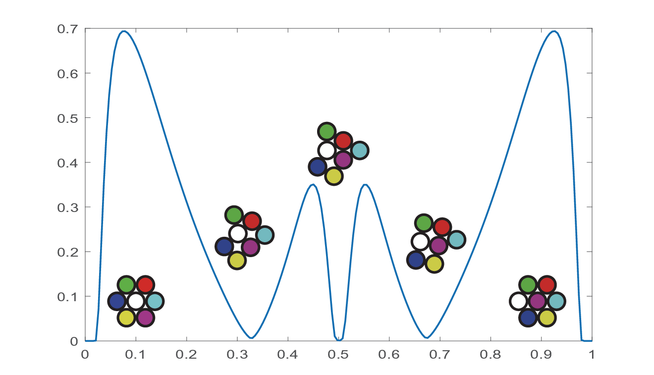
Refer to caption
Figure 6: (Color Online). The indicator λ⁡(α)\lambda(\alpha) for the MPP and the corresponding λ\lambda-critical states when ε=0\varepsilon=0 (i.e. the FW functional). The λ\lambda-critical states are the states where λ\lambda attains local minima.

fig. 7 shows the indicator λ⁡(α)\lambda(\alpha) along the path obtained with ε=0.01\varepsilon=0.01. As we have mentioned, each local minimum of λ\lambda corresponds to a λ\lambda-critical state. These states have different interpretations. The initial and final states, which correspond to the case where one atom is surrounded by the other six, are the minimum of λ\lambda. This means that they are more stable than the other three λ\lambda-critical states. Similarly, the symmetric state (observe with a small tilt angle) in the middle of the path is more stable than another two asymmetric ones aside. Because ε\varepsilon is quite small here, the λ\lambda-critical state we get are similar as those obtained by FW theory.
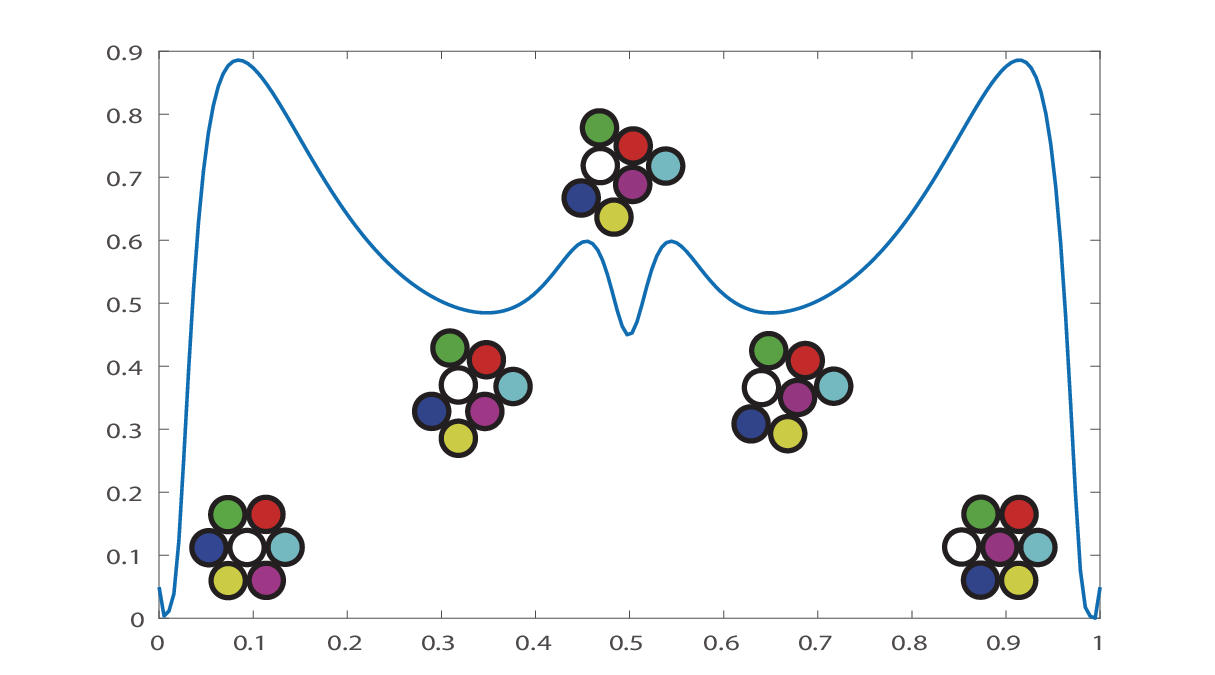
Refer to caption
Figure 7: (Color Online). The indicator λ⁡(α)\lambda(\alpha) for the MPP and the corresponding λ\lambda-critical states when ε=0.01\varepsilon=0.01. The transition behavior resembles the case when ε=0\varepsilon=0.

We also applied EGMA to the cases ε=0.1\varepsilon=0.1 and ε=1\varepsilon=1, and the numerical results are shown in Figs. fig. 8 and fig. 9, respectively. In fig. 8, we observe similar transition pattern as in the case ε=0.01\varepsilon=0.01. Although the critical points of UU that the path goes through are slightly perturbed from the initial and final states, their configurations are qualitatively indistinguishable from those states. The symmetric state in the middle remains to be a λ\lambda-critical state as a local minimum of the indicator λ\lambda. In the case ε=1\varepsilon=1 (shown in Fig, fig. 9)), the two asymmetric states inside replace the initial and final states as the critical states. Furthermore, the middle symmetric state is no longer a λ\lambda-critical state. During the transition, the atoms have slight overlapping due to strong noise perturbations. Similar phenomena was also observed in [30].
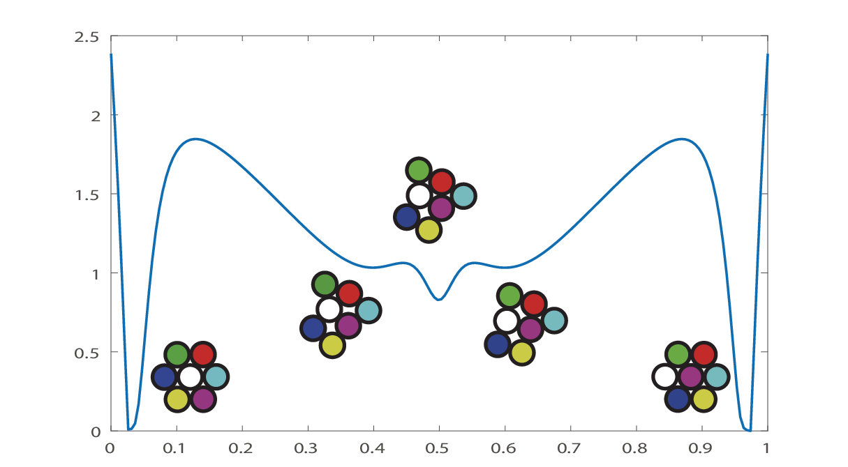
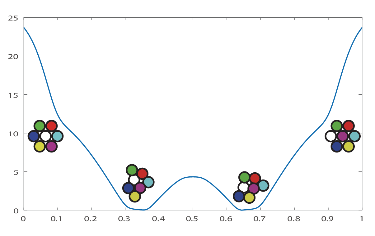
Refer to caption
Figure 8: (Color Online). The indicator λ⁡(α)\lambda(\alpha) for the MPP and the corresponding λ\lambda-critical states when ε=0.1\varepsilon=0.1. The qualitative behavior remains unchanged compared with the case ε=0.01\varepsilon=0.01.
Refer to caption
Figure 9: (Color Online). The indicator λ⁡(α)\lambda(\alpha) for the MPP and the corresponding λ\lambda-critical states when ε=1\varepsilon=1. The two asymmetric states shown in the figure replace the initial and final states as the critical states. The atoms slightly overlap due to the strong noise.

6.3 The Maier-Stein model

In this example, we apply the numerical method to a non-gradient system. The Maier-Stein model is a standard non-gradient diffusion process that has been carefully studied [27]. The drift term 𝒃\bm{b} in Eq. (1) is

𝒃⁡(x,y)=[x−x3−β​x​y2−(1+x2)​y],\bm{b}(x,y)=\begin{bmatrix}x-x^{3}-\beta xy^{2}\\ -(1+x^{2})y\end{bmatrix}, (77)

where β>0\beta>0 is a parameter. The system is of the gradient type only when β=1\beta=1. For any β>0\beta>0, the deterministic dynamics 𝒙˙=𝒃⁡(𝒙)\dot{\bm{x}}=\bm{b}(\bm{x}) has two stable fixed points at (±1,0)(\pm 1,0) and one saddle point at (0,0)(0,0). The path potential U⁡(x,y)U(x,y) is given by

U⁡(x,y)=4​ε​x2+ε​β​y2−12​[(x−x3−β​x​y2)2+(1+x2)2​y2].U(x,y)=4\varepsilon x^{2}+\varepsilon\beta y^{2}-\frac{1}{2}\big[(x-x^{3}-\beta xy^{2})^{2}+(1+x^{2})^{2}y^{2}\big]. (78)

In the limit ε→0\varepsilon\to 0, Maier and Stein studied the transition path from (−1,0)(-1,0) to (1,0)(1,0) for various β\beta, and found two transition patterns [27]. When β<4\beta<4, the path is the line segment connecting (−1,0)(-1,0) and (1,0)(1,0), while when β>4\beta>4, the path is composed of two parts: one from (−1,0)(-1,0) to (0,0)(0,0) following the curved heteroclinic orbit and the other from (0,0)(0,0) to (0,1)(0,1) following the line segment.

Using EGMA, we can study the same transition for ε>0\varepsilon>0. fig. 10 shows the numerical results for ε=0.1\varepsilon=0.1. We also obtain two types of transition paths. However, the critical value of β\beta that separates the two pattens is lowered to a value between 3.4 and 3.5. More interestingly, as predicted by the theoretical result, the paths now pass through a critical point (xc,0)(x_{c},0) which is located to the left of (−1,0)(-1,0).

Refer to caption
Figure 10: (Color Online). The MPP of the OM functional for the Maier-Stein model, where xs=(−1,0)x_{s}=(-1,0), xf=(1,0)x_{f}=(1,0) and ε=0.1\varepsilon=0.1. Left panel: β=3.4\beta=3.4. Right panel: β=3.5\beta=3.5. Blue circles are fixed points of 𝒙˙=𝒃⁡(𝒙)\dot{\bm{x}}=\bm{b}(\bm{x}). Green diamonds are local maximum points of U⁡(x)U(x). The background is the heat map of U⁡(𝒙)U(\bm{x}).

The critical point (xc,0)(x_{c},0) can be calculated explicitly as xc2=(2+1+24​ε)/3x_{c}^{2}=(2+\sqrt{1+24\varepsilon})/3. The corresponding energy is given by Ec=U⁡(xc,0)E_{c}=U(x_{c},0). This helps us study the convergence property of our EGMA. We set ε=0.1\varepsilon=0.1, δ​s=0.01\delta s=0.01, β=10\beta=10 and run 500 iterations with different spatial resolution NN. We compute the difference between EcE_{c} and EnE_{n} in each iteration step. The convergence history of the energy in the first 100 iterations is shown in the upper part of Table 1 when N=1000N=1000. We observe that EnE_{n} increases monotonically towards EcE_{c}. A quantitative fitting shows that |En−Ec|≈O⁡(n−2)+eN|E_{n}-E_{c}|\approx O(n^{-2})+e_{N}, where eNe_{N} is the difference of the limit of EnE_{n}, denoted by EN⋆E^{\star}_{N}, and EcE_{c}. The error eNe_{N} is mainly determined by the spatial resolution NN, which is also shown in Table 1. A fitting shows that |EN⋆−Ec|≈O⁡(h2.314)|E^{\star}_{N}-E_{c}|\approx O(h^{2.314}). This suggests approximately second order convergence of the energy parameter with second order spatial discretization. We will leave the rigorous convergence analysis to the future study.

Table 1: Upper part: Convergence of energy parameter with respect to the iteration number nn. Lower part: Convergence of the limit energy with respect to the spatial resolution NN.
IterNum nn 10 20 30 50 100
Ec−EnE_{c}-E_{n} 2.1×10−32.1\times 10^{-3} 3.9×10−43.9\times 10^{-4} 1.5×10−41.5\times 10^{-4} 8.1×10−58.1\times 10^{-5} 6.2×10−56.2\times 10^{-5}
SpatialRes NN 100 1000 2000 4000 5000
Ec−EN⋆E_{c}-E^{\star}_{N} 6.0×10−56.0\times 10^{-5} 2.0×10−52.0\times 10^{-5} 3.0×10−63.0\times 10^{-6} 1.2×10−71.2\times 10^{-7} 5.3×10−95.3\times 10^{-9}

From Eq. (78) we have

U⁡(0,y)=(ε​β−12)​y2,U(0,y)=(\varepsilon\beta-\frac{1}{2})y^{2},

which shows that U⁡(x,y)U(x,y) is unbound along the yy-axis when ε​β>12\varepsilon\beta>\frac{1}{2}. This violates the Assumption 2. In principle this is beyond our theoretical framework. But it is still interesting to apply EGMA in this case. Based on the result in Proposition 3.6, the energy parameter EE will tend to infinity while the path may diverge along yy-axis. The numerical results confirm this conjecture, although the current theory does not cover this case. The divergent curves are shown in fig. 11.

Refer to caption
Figure 11: (Color Online). Divergence of the yy-component of φn​(α)\varphi^{n}(\alpha) in the iterations when ε​β>12\varepsilon\beta>\frac{1}{2}. Here we choose ε=1\varepsilon=1, β=10\beta=10.

7 Conclusion and discussion

In this paper, we studied the minimization problem of the OM functional STOM​[ψ]S^{{\rm OM}}_{T}[\psi] when TT tends to infinity. Under mild conditions, we rigorously showed that the infimum of STOM​[ψ]S^{{\rm OM}}_{T}[\psi] over ψ\psi and TT is always −∞-\infty and it occurs only when T→+∞T\to+\infty. Moreover, we proved that when T→+∞T\to+\infty, the minimizer of STOM​[ψ]S^{{\rm OM}}_{T}[\psi] has convergent subsequence in the configuration space. With the help of Maupertuis principle, the problem of finding the graph limit of the minimizers of the OM functional is translated into that of finding an extremal of S^E​[φ]\hat{S}_{E}[\varphi] with the energy E⋆=max𝒙⁡U⁡(𝒙)E^{\star}=\max_{\bm{x}}U(\bm{x}), where UU is the path potential.

Based on these theoretical results, we designed an efficient algorithm (EGMA) to find the energy E⋆E^{\star} and solve the Euler-Lagrange equation simultaneously. This algorithm can be viewed as a nontrivial extension of the geometric minimum action method (gMAM), which was proposed for the double minimization problem of the FW functional at zero temperature [22]. In gMAM, the energy EE is fixed at zero, and the corresponding optimal transition time T=∫01(2​E−2​U​(φ))−12​|φ′|​𝑑αT=\int_{0}^{1}(2E-2U(\varphi))^{-\frac{1}{2}}\left|\varphi^{\prime}\right|\,\mathrm{d}\alpha can be either finite or infinite. We note that the method can be extended to the case of non-zero EE, which corresponds to a prescribed value for the transition time. In EGMA, the energy changes step by step to ensure that the time TT always goes to infinity. This algorithm was successfully applied to several typical rare event examples. Although the rigorous proof of the convergence of the algorithm is still absent, our numerical examples in Sections 6.1 and 6.2 demonstrated that it converges to an extremal of S^E⋆​[φ]\hat{S}_{E^{\star}}[\varphi] in practice.

Some possible extensions and unsolved problems arise naturally based on the theoretical analysis of the current paper. Below we list some of them.

  1. (i)

    As mentioned in the remarks, the conclusions that infTinfψSTOM​[ψ]=−∞\inf_{T}\inf_{\psi}S^{{\rm OM}}_{T}[\psi]=-\infty and the minimizer of STOM​[ψ]S^{{\rm OM}}_{T}[\psi] has convergent subsequence in the configuration space can be generalized to non-gradient systems with drift 𝒃⁡(𝒙)\bm{b}(\bm{x}) under suitable assumptions. However, the proof of the key result that φ⋆\varphi^{\star} is an extremal of S^E⋆​[φ]\hat{S}_{E^{\star}}[\varphi] relies on the gradient form of 𝒃⁡(𝒙)\bm{b}(\bm{x}). Indeed, the proof of Lemma A.1 holds because the value of S^E​[φ]\hat{S}_{E}[\varphi] is non-negative. Besides, we used an analog of Hartman-Grobman theorem to transfer the uniform BV property of φk′\varphi_{k}^{\prime} for linearized problem to the non-linear case in the neighborhood of the critical point 𝒙c\bm{x}_{c}. This approach requires that (𝒙c,0)(\bm{x}_{c},0) is a hyperbolic fixed point of the first order system (85). For non-gradient case, the first order system (85) becomes

    Ψ˙1\displaystyle\dot{\Psi}_{1} =Ψ2,\displaystyle=\Psi_{2}, (79)
    Ψ˙2\displaystyle\dot{\Psi}_{2} =−∇2U​(Ψ1)−(∇𝒃T​(Ψ1)−∇𝒃​(Ψ1))​Ψ2.\displaystyle=-\nabla^{2}U(\Psi_{1})-(\nabla\bm{b}^{\mathrm{T}}(\Psi_{1})-\nabla\bm{b}(\Psi_{1}))\Psi_{2}.

    The point (𝒙c,0)(\bm{x}_{c},0) is still a fixed point. However, the eigenvalues of the Jacobian of (79) at (𝒙c,0)(\bm{x}_{c},0) have non-zero imaginary past. To study the behavior of φk′\varphi_{k}^{\prime} near the critical point, we might need more delicate study of the dynamics (79) on center manifold and more advanced result on linearization. So how to extend Theorem 3.13 to the non-gradient case remains an interesting issue.

  2. (ii)

    Presumably, the Freidlin-Wentzell functional can be viewed as a limit of Onsager-Machlup functional when ε→0\varepsilon\to 0. However, we have limε→0infT\lim_{\varepsilon\to 0}\inf_{T} infψSTOM​[ψ]=−∞\inf_{\psi}S^{{\rm OM}}_{T}[\psi]=-\infty by the Proposition 3.8. This suggests that a naive process is not valid to establish such connection. A possible alternative to investigate the limit of OM functional is to relate TT and ε\varepsilon by a function T=T⁡(ε)T=T(\varepsilon) and study the convergence of infψST⁡(ε)OM​[ψ]\inf_{\psi}S^{{\rm OM}}_{T(\varepsilon)}[\psi] as ε→0\varepsilon\to 0. This idea has been partially studied in [31]. They showed that for the scaling T=ε−αT=\varepsilon^{-\alpha}, 0<α⩽10<\alpha\leqslant 1, the OM functional Γ\Gamma-converges to a functional completely characterized by the FW theory. However, for a more general and physical scaling T=T⁡(ε)T=T(\varepsilon), the convergence of OM functional and its minimizer is not clear. The renormalized OM functional (9) might be a good candidate to perform such analysis.

  3. (iii)

    The discretization scheme described in EGMA can be further improved. For example, one may discretize S^E​[φ]\hat{S}_{E}[\varphi] first then use some optimization methods like quasi-Newton or conjugate gradient type methods to search for the extremal. However, the algorithm we proposed here combines the iteration for solving Euler-Lagrange equation and finding the maximum of U⁡(𝒙)U(\bm{x}) simultaneously. It has the advantage that we can compute the optimal energy parameter and the MPP at the same time. This strategy may not apply for the optimization methods. Designing more efficient numerical methods to perform these two tasks together is an issue of practical interests.

In summary, the current work provides new ideas on the FW-OM dilemma. It will be instructive to further study the FW-OM connections with this new perspective.

\Acknowledgements

The authors are grateful to Profs. Shaobo Gan, Eric Vanden-Eijnden, Jiazhong Yang and Shulin Zhou for stimulating discussions. Special thanks are due to Prof. Wenmeng Zhang for his patient explanation about their recent progress on C1,βC^{1,\beta}-linearization problem. The work of T. Li is supported by the NSFC under grants No. 11421101, 91530322 and 11825102. The work of W. Ren is partially supported by Singapore MOE ACRF grants R-146-000-267-114 (Tier-1) and R-146-000-232-112 (Tier-2), and NSFC grant No. 11871365. The work of X. Li is supported by the Construct Program of the Key Discipline in Hunan Province.

References

  • [1] V.I. Arnold. Mathematical methods of classical mechanics. Springer-Verlag, Berlin, 1989.
  • [2] A. Bovier, M. Eckhoff, V. Gayrard, and M. Klein. Metastablility in reversible diffusion processes I. Sharp asymptotics for capacities and exit times. J. Eur. Math. Soc., 6:399–424, 2004.
  • [3] A. Bovier, V. Gayrard, and M. Klein. Metastablility in reversible diffusion processes II. Precise asymptotics for small eigenvalues. J. Eur. Math. Soc., 7:69–99, 2005.
  • [4] M. Cameron, R.V. Kohn, and E. Vanden-Eijnden. The string method as a dynamical system. J. Nonlinear Sci., 21:193–230, 2011.
  • [5] G. Contreras, J. Delgado, and R. Iturriaga. Lagrangian flows: The dynamics of globally minimizing orbits-II. Bull. Braz. Math. Soc., 28(2):155–196, 1997.
  • [6] C.M. Dafermos. Hyperbolic conservation laws in continuum physics. Springer, Berlin and Heidelberg, 3rd edition, 2010.
  • [7] C. Dellago, P.G. Bolhuis, and D. Chandler. Efficient transition path sampling: Application to Lennard-Jones cluster rearrangements. J. Chem. Phys., 108(22):9236–9245, 1998.
  • [8] M.M. Dunlop and A.M. Stuart. MAP estimators for piecewise continuous inversion. Inverse. Probl., 32(10), 2016.
  • [9] D. Dürr and A. Bach. The Onsager-Machlup function as Lagrangian for the most probable path of a diffusion process. Commun. Math. Phys., 60(2):153–170, 1978.
  • [10] W. E, W. Ren, and E. Vanden-Eijnden. String method for the study of rare events. Phys. Rev. B, 66(5):052301, 2002.
  • [11] W. E, W. Ren, and E. Vanden-Eijnden. Minimum action method for the study of rare events. Comm. Pure. Appl. Math., 57:637–656, 2004.
  • [12] W. E, W. Ren, and E. Vanden-Eijnden. Simplified and improved string method for computing the minimum energy paths in barrier-crossing events. J. Chem. Phys., 126(16):164103, 2007.
  • [13] W. E and E. Vanden-Eijnden. Towards a theory of transition paths. J. Stat. Phys., 123(3), 2006.
  • [14] W. E and E. Vanden-Eijnden. Transition-path theory and path-finding algorithms for the study of rare events. Ann. Rev. Phys. Chem., 61:391–420, 2010.
  • [15] P. Faccioli, M. Sega, F. Pederiva, and H. Orland. Dominant pathways in protein folding. Phys. Rev. Lett., 97(10):108101, 2006.
  • [16] H. Fujisaki, M. Shiga, and A. Kidera. Onsager–Machlup action-based path sampling and its combination with replica exchange for diffusive and multiple pathways. J. Chem. Phys., 132(13):134101, 2010.
  • [17] H. Fujisaki, M. Shiga, K. Moritsugu, and A. Kidera. Multiscale enhanced path sampling based on the Onsager-Machlup action: Application to a model polymer. J. Chem. Phys., 139(5):054117, 2013.
  • [18] T. Fujita and S. Kotani. The Onsager-Machlup function for diffusion processes. J. Math. Kyoto Univ., 22:115–130, 1982.
  • [19] M. Giaquinta and S. Hildebrandt. Calculus of variations I. Springer Science & Business Media, Berlin, 2004.
  • [20] R. Graham. Path integral formulation of general diffusion processes. Z. Physik B, 26:281–290, 1977.
  • [21] P. Hänggi, P. Talkner, and M. Borkovec. Reaction-rate theory: Fifty years after Kramers. Rev. Mod. Phys., 62:251–342, 1990.
  • [22] M. Heymann and E. Vanden-Eijnden. The geometric minimum action method: A least action principle on the space of curves. Comm. Pure. Appl. Math., 61(8):1052–1117, 2008.
  • [23] N. Ikeda and S. Watanabe. Stochastic differential equations and diffusion processes. Wiley, New York, 1980.
  • [24] L.D. Landau and E.M. Lifshitz. Mechanics, volume 1 of Course of Theoretical Physics. Butterworth-Heinemann, Oxford, 3rd edition edition, 1999.
  • [25] J. Lee, I. Lee, I. Joung, J. Lee, and B.R. Brooks. Finding dominant reaction pathways via global optimization of action. Biophys. J., 112(3):290a, 2017.
  • [26] C. Lv, X. Li, F. Li, and T. Li. Constructing the energy landscape for genetic switching system driven by intrinsic noise. PLoS One, 9:e88167, 2014.
  • [27] R.S. Maier and D.L. Stein. A scaling theory of bifurcations in the symmetric weak-noise escape problem. J. Stat. Phys., 83(3-4):291–357, 1996.
  • [28] R. Mané. Lagrangian flows: The dynamics of globally minimizing orbits. Bull. Braz. Math. Soc., 28(2):141–153, 1997.
  • [29] L. Onsager and S. Machlup. Fluctuations and irreversible processes. Phys. Rev., 91(6):1505, 1953.
  • [30] F.J. Pinski and A.M. Stuart. Transition paths in molecules at finite temperature. J. Chem. Phys., 132(18):184104, 2010.
  • [31] F.J. Pinski, A.M. Stuart, and F. Theil. Γ\Gamma-limit for transition paths of maximal probability. J. Stat. Phys., 146(5):955–974, 2012.
  • [32] C. Schütte and M. Sarich. Metastability and Markov state models in molecular dynamics: modeling, analysis, algorithmic approaches, volume 24 of Courant Lecture Notes. Amer. Math. Soc., Providence, 2013.
  • [33] Y. Takahashi and S. Watanabe. The probability functionals (Onsager-Machlup functions) of diffusion processes. In Stochastic Integrals, pages 433–463. Springer, 1981.
  • [34] X. Wan. An adaptive high-order minimum action method. J. Comp. Phys., 230:8669–8682, 2011.
  • [35] J. Wang, K. Zhang, and E. Wang. Kinetic paths, time scale, and underlying landscapes: A path integral framework to study global natures of nonequilibrium systems and networks. J. Chem. Phys., 133(12):125103, 2010.
  • [36] O. Zeitouni. On the Onsager-Machlup functional of diffusion processes around non C2C^{2} curves. Ann. Prob., 17(3):1037–1054, 1989.
  • [37] L. Zhang, W. Ren, A. Samanta, and Q. Du. Recent developments in computational modelling of nucleation in phase transformations. NPJ Comput. Mater., 2:16003, 2016.
  • [38] W. Zhang, K. Lu, and W. Zhang. Differentiability of the conjugacy in the Hartman-Grobman theorem. Trans. Amer. Math. Soc., 369:4995–5030, 2017.
  • [39] P. Zhou and T. Li. Construction of the landscape for multi-stable systems: Potential landscape, quasi-potential, A-type integral and beyond. J. Chem. Phys., 144(9):094109, 2016.
  • [40] X. Zhou, W. Ren, and W. E. Adaptive minimum action method for the study of rare events. J. Chem. Phys., 128(10):104111, 2008.

Appendix A Proof of Proposition 3.14

We now prove Proposition 3.14 in this Appendix. This relies on a series of lemmas. Some of them are quite technical. Recall that ψk\psi_{k} is the minimizer of STkOM​[ψ]S^{{\rm OM}}_{T_{k}}[\psi], where Tk→+∞T_{k}\to+\infty as k→∞k\to\infty. The corresponding energy Ek=E⁡(Tk)E_{k}=E(T_{k}) and the extremal of S^Ek​[φ]\hat{S}_{E_{k}}[\varphi] is φk\varphi_{k} for k=1,2,…k=1,2,\dots. By theorem 3.11, we may assume Ek→E⋆E_{k}\to E^{\star} and φk→φ⋆\varphi_{k}\to\varphi^{\star} without loss of generality.

Our main idea is to show that each component of {φk′}\{\varphi_{k}^{\prime}\} has uniformly bounded variations. Denote φk′(i)\varphi_{k}^{\prime(i)} the iith component of φk′\varphi^{\prime}_{k}. We have the total variation

⋁01φk′(i)​(α)\displaystyle\bigvee\limits_{0}^{1}\varphi_{k}^{\prime(i)}(\alpha) =supΔ∑j=0n|φk′(i)​(αj+1)−φk′(i)​(αj)|\displaystyle=\sup\limits_{\Delta}\sum_{j=0}^{n}\big|\varphi_{k}^{\prime(i)}(\alpha_{j+1})-\varphi_{k}^{\prime(i)}(\alpha_{j})\big| (80)
⩽supΔ∑i=1d∑j=0n|φk′(i)​(αj+1)−φk′(i)​(αj)|\displaystyle\leqslant\sup\limits_{\Delta}\sum_{i=1}^{d}\sum_{j=0}^{n}\big|\varphi_{k}^{\prime(i)}(\alpha_{j+1})-\varphi_{k}^{\prime(i)}(\alpha_{j})\big|
⩽supΔ∑j=0nd​(∑i=1d|φk′(i)​(αj+1)−φk′(i)​(αj)|2)12\displaystyle\leqslant\sup\limits_{\Delta}\sum_{j=0}^{n}\sqrt{d}\left(\sum_{i=1}^{d}\big|\varphi_{k}^{\prime(i)}(\alpha_{j+1})-\varphi_{k}^{\prime(i)}(\alpha_{j})\big|^{2}\right)^{\frac{1}{2}}
=supΔ∑j=0nd​|φk′​(αj+1)−φk′​(αj)|,\displaystyle=\sup\limits_{\Delta}\sum_{j=0}^{n}\sqrt{d}\left|\varphi^{\prime}_{k}(\alpha_{j+1})-\varphi^{\prime}_{k}(\alpha_{j})\right|,

where Δ\Delta is a partition of [0,1][0,1] with subdivision points 0=α0<α1<α2​⋯<αn+1=10=\alpha_{0}<\alpha_{1}<\alpha_{2}\dots<\alpha_{n+1}=1. We only need to show that

supΔ∑j=0n|φk′​(αj+1)−φk′​(αj)|\sup\limits_{\Delta}\sum_{j=0}^{n}\left|\varphi^{\prime}_{k}(\alpha_{j+1})-\varphi^{\prime}_{k}(\alpha_{j})\right| (81)

is uniformly bounded.

Next, we divide [0,1][0,1] into intervals in which φk∈C2\varphi_{k}\in C^{2}. We need the following lemma.

Lemma A.1.

There is a constant K>0K>0 which is independent of TT, such that for any T>0T>0, #⁡{t∈[0,T]|U⁡(ψT​(t))=E⁡(T)}⩽K\#\{t\in[0,T]|U(\psi_{T}(t))=E(T)\}\leqslant K.

Proof A.2.

By Assumption 2, we have the decomposition

{𝒙|U⁡(𝒙)=E⁡(T)}=⋃i=1NBi,\Big\{\bm{x}|U(\bm{x})=E(T)\Big\}=\bigcup\limits_{i=1}^{N}B_{i},

where Bi∩Bj=∅B_{i}\cap B_{j}=\emptyset for i≠ji\neq j, BiB_{i} is closed and connected. We are going to show that ψT\psi_{T} passes through each BiB_{i} at most once.

Assume that there exist 0<t1<t2<T0<t_{1}<t_{2}<T such that 𝐱1=ψT​(t1)∈Bi\bm{x}_{1}=\psi_{T}(t_{1})\in B_{i}, 𝐱2=ψT​(t2)∈Bi\bm{x}_{2}=\psi_{T}(t_{2})\in B_{i}. Define ψ~T~​(t)=ψT​(t+t1)\tilde{\psi}_{\tilde{T}}(t)=\psi_{T}(t+t_{1}) for t∈[0,t2−t1]t\in[0,t_{2}-t_{1}], where T~=t2−t1\tilde{T}=t_{2}-t_{1}. ψ~T~\tilde{\psi}_{\tilde{T}} must be the minimizer of ST~​[ψ]S_{\tilde{T}}[\psi] with boundary conditions ψ⁡(0)=𝐱1\psi(0)=\bm{x}_{1}, ψ⁡(T~)=𝐱2\psi(\tilde{T})=\bm{x}_{2}. Since ψ~T~\tilde{\psi}_{\tilde{T}} is the minimizer of ST~​[ψ]S_{\tilde{T}}[\psi], by Maupertuis principle we know that the minimizer ψ~T~\tilde{\psi}_{\tilde{T}} induces a geodesic on BiB_{i} from 𝐱1\bm{x}_{1} to 𝐱2\bm{x}_{2} with Riemannian metric [1](Theorem in page 246)

d​ρE=2​E​(T)−U⁡(φ)​|d​φ|.\,\mathrm{d}\rho_{E}=\sqrt{2E(T)-U(\varphi)}\left|d\varphi\right|.

ψ~T~\tilde{\psi}_{\tilde{T}} must lie on BiB_{i} since it minimizes the distance induced by ρE\rho_{E}. However, we have

T⩾∫𝒙1𝒙2|d​ψ~T~|2​E​(T)−2​U​(ψ~T~)=+∞.T\geqslant\int_{\bm{x}_{1}}^{\bm{x}_{2}}\frac{\left|\,\mathrm{d}\tilde{\psi}_{\tilde{T}}\right|}{\sqrt{2E(T)-2U(\tilde{\psi}_{\tilde{T}})}}=+\infty.

This contradiction implies that ψT\psi_{T} passes through BiB_{i} at most once.

Since there are only finite components BiB_{i} of level set {𝐱|U⁡(𝐱)=E⁡(T)}\{\bm{x}|U(\bm{x})=E(T)\}, there is a positive lower bound of the distance between each two components

mini≠j⁡dist​(Bi,Bj)=l>0.\min\limits_{i\neq j}\mbox{dist}(B_{i},B_{j})=l>0.

By Assumption 2, the length of ψT\psi_{T} is uniformly bounded. So we have for any T>0T>0,

M⩾∫0T|ψ˙T|​𝑑t⩾(K−1)​l.M\geqslant\int_{0}^{T}|\dot{\psi}_{T}|\,\mathrm{d}t\geqslant(K-1)l.

This leads to the conclusion that KK is finite and independent of TT.

Lemma A.1 shows that for any kk, the points α\alpha satisfying U⁡(φk​(α))=EkU(\varphi_{k}(\alpha))=E_{k} are finite. Note that when U⁡(φk​(α))<EkU(\varphi_{k}(\alpha))<E_{k}, φk∈C2\varphi_{k}\in C^{2}. By Euler-Lagrange equation (33), in an interval [β1,β2][\beta_{1},\beta_{2}] such that φk∈C2\varphi_{k}\in C^{2}, the total variation of φk′\varphi_{k}^{\prime} is

⋁β1β2φk(i)⩽∫β1β2|φk′′|​𝑑α=∫β1β2|φk′|​|∇U|2​|φk′|2−⟨∇U,φk′⟩22​Ek−2​U​(φk)​𝑑α.\bigvee_{\beta_{1}}^{\beta_{2}}\varphi_{k}^{(i)}\leqslant\int_{\beta_{1}}^{\beta_{2}}\left|\varphi_{k}^{\prime\prime}\right|\,\mathrm{d}\alpha=\int_{\beta_{1}}^{\beta_{2}}\frac{\left|\varphi_{k}^{\prime}\right|\sqrt{\left|\nabla U\right|^{2}\left|\varphi_{k}^{\prime}\right|^{2}-\left\langle\nabla U,\varphi_{k}^{\prime}\right\rangle^{2}}}{2E_{k}-2U(\varphi_{k})}\,\mathrm{d}\alpha. (82)

We can rewrite Eq. (82) with time parameterization as

∫β1β2|φk′′|​dα=\displaystyle\int_{\beta_{1}}^{\beta_{2}}\left|\varphi_{k}^{\prime\prime}\right|\,\mathrm{d}\alpha= ∫β1β2|φk′|​|∇U|2​|φk′|2−⟨∇U,φk′⟩22​Ek−2​U​(φk)​𝑑α\displaystyle\int_{\beta_{1}}^{\beta_{2}}\frac{\left|\varphi_{k}^{\prime}\right|\sqrt{\left|\nabla U\right|^{2}\left|\varphi_{k}^{\prime}\right|^{2}-\left\langle\nabla U,\varphi_{k}^{\prime}\right\rangle^{2}}}{2E_{k}-2U(\varphi_{k})}\,\mathrm{d}\alpha (83)
=∫β1β2|φk′|2​|∇U|2​|τ^k|2−⟨∇U,τ^k⟩22​Ek−2​U​(φk)​𝑑α\displaystyle=\int_{\beta_{1}}^{\beta_{2}}\frac{\left|\varphi_{k}^{\prime}\right|^{2}\sqrt{\left|\nabla U\right|^{2}\left|\hat{\tau}_{k}\right|^{2}-\left\langle\nabla U,\hat{\tau}_{k}\right\rangle^{2}}}{2E_{k}-2U(\varphi_{k})}\,\mathrm{d}\alpha
=∫t1t2|φk′|2​|∇U|2​|ψ˙k|2−⟨∇U,ψ˙k⟩2|ψ˙k|3​d​αd​t​𝑑t\displaystyle=\int_{t_{1}}^{t_{2}}\frac{\left|\varphi_{k}^{\prime}\right|^{2}\sqrt{\left|\nabla U\right|^{2}|\dot{\psi}_{k}|^{2}-\langle\nabla U,\dot{\psi}_{k}\rangle^{2}}}{|\dot{\psi}_{k}|^{3}}\frac{\,\mathrm{d}\alpha}{\,\mathrm{d}t}\,\mathrm{d}t
=|φk′|​∫t1t2|∇U|2​|ψ˙k|2−⟨∇U,ψ˙k⟩2|ψ˙k|4​dt,\displaystyle=\left|\varphi_{k}^{\prime}\right|\int_{t_{1}}^{t_{2}}\sqrt{\frac{\left|\nabla U\right|^{2}|\dot{\psi}_{k}|^{2}-\langle\nabla U,\dot{\psi}_{k}\rangle^{2}}{|\dot{\psi}_{k}|^{4}}}\,\mathrm{d}t,

where τ^k=φk′/|φk′|\hat{\tau}_{k}=\varphi_{k}^{\prime}/|\varphi_{k}^{\prime}|, t1=ℓ−1​(β1)t_{1}=\ell^{-1}(\beta_{1}) and t2=ℓ−1​(β2)t_{2}=\ell^{-1}(\beta_{2}).

For any T>0T>0, we define

ΘT​(t)=|∇U​(ψT)|2​|ψ˙T|2−⟨∇U​(ψT),ψ˙T⟩2|ψ˙T|4\Theta_{T}(t)=\frac{\left|\nabla U(\psi_{T})\right|^{2}|\dot{\psi}_{T}|^{2}-\langle\nabla U(\psi_{T}),\dot{\psi}_{T}\rangle^{2}}{|\dot{\psi}_{T}|^{4}} (84)

and denote Θk​(t)=ΘTk​(t)\Theta_{k}(t)=\Theta_{T_{k}}(t). It is obvious that ΘT​(t)\Theta_{T}(t) is well-defined for U⁡(ψT​(t))<E⁡(T)U(\psi_{T}(t))<E(T). Recall that the minimizer ψT\psi_{T} satisfies the Euler-Lagrange equation

ψ¨+∇U​(ψ)=0,\ddot{\psi}+\nabla U(\psi)=0,

or equivalently the first order system

Ψ˙1\displaystyle\dot{\Psi}_{1} =Ψ2,\displaystyle=\Psi_{2}, (85)
Ψ˙2\displaystyle\dot{\Psi}_{2} =−∇U​(Ψ1).\displaystyle=-\nabla U(\Psi_{1}).

We have ψ≡Ψ1\psi\equiv\Psi_{1}. We will use Ψ~\tilde{\Psi} to denote the extended variable (Ψ1,Ψ2)∈ℝ2​d(\Psi_{1},\Psi_{2})\in\mathbb{R}^{2d}. The state Ψ~c=(𝒙c,0)\tilde{\Psi}_{c}=(\bm{x}_{c},0) is a fixed point of the system, where 𝒙c\bm{x}_{c} is a critical point. The following lemma shows that the function ΘT​(t)\Theta_{T}(t) can be continuously extended to t∈[0,T]t\in[0,T].

Lemma A.3 (Preliminary properties of ΘT\Theta_{T} and Ψ\Psi).
  1. (1)

    Given 𝒙s≠𝒙c\bm{x}_{s}\neq\bm{x}_{c}, 𝒙f≠𝒙c\bm{x}_{f}\neq\bm{x}_{c} and T>0T>0, lims→tΘT​(s)\lim_{s\to t}\Theta_{T}(s) exists for any t∈[0,T]t\in[0,T].

  2. (2)

    There exists a neighborhood 𝒰\mathcal{U} of critical point 𝒙c\bm{x}_{c} and constant m>0m>0, such that for any given t0>0t_{0}>0, 𝒙s,𝒙f∈∂𝒰\bm{x}_{s},\bm{x}_{f}\in\partial\mathcal{U}, we have |Ψ2|⩾m>0\left|\Psi_{2}\right|\geqslant m>0 for t∈[0,t0]t\in[0,t_{0}] when T→+∞T\to+\infty.

Proof A.4.

(1) Since Ψ1,Ψ2∈C1​[0,T]\Psi_{1},\Psi_{2}\in C^{1}[0,T], ΘT\Theta_{T} is continuous except the points with Ψ2​(tc)=0\Psi_{2}(t_{c})=0. Below we will show these points are removable singularities.

Suppose Ψ2​(tc)=0\Psi_{2}(t_{c})=0. We have the following Taylor expansion near tct_{c}

−∇U​(Ψ1)\displaystyle-\nabla U(\Psi_{1}) =Ψ(2)+12​Ψ(4)​(t−tc)2+124​Ψ(6)​(t−tc)4+o​(t−tc)5,\displaystyle=\Psi^{(2)}+\frac{1}{2}\Psi^{(4)}(t-t_{c})^{2}+\frac{1}{24}\Psi^{(6)}(t-t_{c})^{4}+o(t-t_{c})^{5}, (86)
Ψ2\displaystyle\Psi_{2} =Ψ(2)​(t−tc)+16​Ψ(4)​(t−tc)3+1120​Ψ(6)​(t−tc)5+o​(t−tc)6,\displaystyle=\Psi^{(2)}(t-t_{c})+\frac{1}{6}\Psi^{(4)}(t-t_{c})^{3}+\frac{1}{120}\Psi^{(6)}(t-t_{c})^{5}+o(t-t_{c})^{6},

where Ψ(2)\Psi^{(2)}, Ψ(4)\Psi^{(4)}, Ψ(6)\Psi^{(6)} are corresponding higher derivatives of Ψ1​(t)\Psi_{1}(t) assuming value at tct_{c}. The odd order derivatives of Ψ1\Psi_{1} disappear because Ψ(1)=0\Psi^{(1)}=0,

Ψ(3)=dd​tΨ1(2)=−dd​t∇U(Ψ1)=−∇2U⋅Ψ˙1=0\Psi^{(3)}=\frac{\,\mathrm{d}\,}{\,\mathrm{d}t}\Psi_{1}^{(2)}=-\frac{\,\mathrm{d}\,}{\,\mathrm{d}t}\nabla U(\Psi_{1})=-\nabla^{2}U\cdot\dot{\Psi}_{1}=0

and

Ψ(5)=dd​tΨ1(4)=dd​t∇2U∇U=∇(∇2U∇U)⋅Ψ˙1=0.\Psi^{(5)}=\frac{\,\mathrm{d}\,}{\,\mathrm{d}t}\Psi_{1}^{(4)}=\frac{\,\mathrm{d}\,}{\,\mathrm{d}t}\nabla^{2}U\nabla U=\nabla(\nabla^{2}U\nabla U)\cdot\dot{\Psi}_{1}=0.

Substituting (86) into ΘT​(t)\Theta_{T}(t), we obtain that in a neighborhood of tct_{c},

ΘT​(t)=(|Ψ(2)|2​|Ψ(4)|2−⟨Ψ(2),Ψ(4)⟩2)​(t−tc)2+o​(t−tc)29​|Ψ(4)|2+o⁡(1).\Theta_{T}(t)=\frac{\big(\left|\Psi^{(2)}\right|^{2}\left|\Psi^{(4)}\right|^{2}-\left\langle\Psi^{(2)},\Psi^{(4)}\right\rangle^{2}\big)(t-t_{c})^{2}+o(t-t_{c})^{2}}{9\left|\Psi^{(4)}\right|^{2}+o(1)}. (87)

With the fact that Ψ(2)=−∇U\Psi^{(2)}=-\nabla U, Ψ(4)=∇2U∇U\Psi^{(4)}=\nabla^{2}U\nabla U taking value at Ψ1​(tc)\Psi_{1}(t_{c}), we have

ΘT​(t)=[∇U^​(∇2U)2​∇U^−(∇U^​∇2U​∇U^)2]​(t−tc)2+o​(t−tc)29+o⁡(1),\Theta_{T}(t)=\frac{[\widehat{\nabla U}(\nabla^{2}U)^{2}\widehat{\nabla U}-(\widehat{\nabla U}\nabla^{2}U\widehat{\nabla U})^{2}](t-t_{c})^{2}+o(t-t_{c})^{2}}{9+o(1)},

where ∇U^=∇U/|∇U|\widehat{\nabla U}=\nabla U/\left|\nabla U\right|. Since Ψ1\Psi_{1} is uniformly bounded, limt→tcΘT​(t)=0\lim_{t\to t_{c}}\Theta_{T}(t)=0. This ends the proof of the first statement.

(2) By assumption 2, all eigenvalues of ∇2U​(𝐱c)\nabla^{2}U(\bm{x}_{c}) are negative, so there is a neighborhood 𝒰\mathcal{U} of 𝐱c\bm{x}_{c}, for any 𝐱∈∂𝒰\bm{x}\in\partial\mathcal{U}, 𝐱≠𝐱c\bm{x}\neq\bm{x}_{c}, U⁡(𝐱)<U⁡(𝐱c)U(\bm{x})<U(\bm{x}_{c}). For 𝐱,𝐲∈ℝd\bm{x},\bm{y}\in\mathbb{R}^{d}, let (Φ1​(t,𝐱,𝐲),Φ2​(t,𝐱,𝐲))(\Phi_{1}(t,\bm{x},\bm{y}),\Phi_{2}(t,\bm{x},\bm{y})) be the solution of (85) at time tt with initial condition Ψ1​(0)=𝐱\Psi_{1}(0)=\bm{x}, Ψ2​(0)=𝐲\Psi_{2}(0)=\bm{y}. So Ψ1​(t)=Φ1​(t,𝐱s,𝐲s​(T))\Psi_{1}(t)=\Phi_{1}(t,\bm{x}_{s},\bm{y}_{s}(T)), Ψ2​(t)=Φ2​(t,𝐱s,𝐲s​(T))\Psi_{2}(t)=\Phi_{2}(t,\bm{x}_{s},\bm{y}_{s}(T)) for some proper 𝐲s\bm{y}_{s}. Conservation of energy implies

|𝒚s|2=2​E​(T)−2​U​(𝒙s).\left|\bm{y}_{s}\right|^{2}=2E(T)-2U(\bm{x}_{s}). (88)

From E⁡(T)→E⋆E(T)\to E^{\star}, 𝐱s\bm{x}_{s} assumes value on a compact set ∂𝒰\partial\mathcal{U}, we know |𝐲s|2⩽2​(E⋆+1)+2​max𝐱s∈∂𝒰⁡U⁡(𝐱s)\left|\bm{y}_{s}\right|^{2}\leqslant 2(E^{\star}+1)+2\max_{\bm{x}_{s}\in\partial\mathcal{U}}U(\bm{x}_{s}) for large enough TT.

Because Φ1​(t,𝐱,𝐲)\Phi_{1}(t,\bm{x},\bm{y}), Φ2​(t,𝐱,𝐲)\Phi_{2}(t,\bm{x},\bm{y}) are continuous functions of (t,𝐱,𝐲)(t,\bm{x},\bm{y}), the triple (t,𝐱,𝐲)(t,\bm{x},\bm{y}) assumes value in a compact set [0,t0]×∂𝒰×{|𝐲|⩽2(E⋆+1)+2max𝐱s∈∂𝒰U(𝐱s)}[0,t_{0}]\times\partial\mathcal{U}\times\{\left|\bm{y}\right|\leqslant 2(E^{\star}+1)+2\max_{\bm{x}_{s}\in\partial\mathcal{U}}U(\bm{x}_{s})\}, the continuous function |Φ1−𝐱c|2+|Φ2|2\left|\Phi_{1}-\bm{x}_{c}\right|^{2}+\left|\Phi_{2}\right|^{2} has a minimum mm. Note that (𝐱c,0)(\bm{x}_{c},0) is a fixed point of (85), the minimum mm must be positive, otherwise the uniqueness of initial value problem will be violated. So we have

|Φ1​(t,𝒙s,𝒚s)−𝒙c|2+|Φ2​(t,𝒙s,𝒚s)|2⩾m>0.\left|\Phi_{1}(t,\bm{x}_{s},\bm{y}_{s})-\bm{x}_{c}\right|^{2}+\left|\Phi_{2}(t,\bm{x}_{s},\bm{y}_{s})\right|^{2}\geqslant m>0. (89)

Let tm​(T)=arg⁡mint∈[0,t0]​|Φ2​(t,𝐱s,𝐲s​(T))|t_{m}(T)=\arg\min_{t\in[0,t_{0}]}\left|\Phi_{2}(t,\bm{x}_{s},\bm{y}_{s}(T))\right|, we have

lim infT→+∞|Φ2​(tm​(T),𝒙s,𝒚s​(T))|>0.\liminf_{T\to+\infty}\left|\Phi_{2}(t_{m}(T),\bm{x}_{s},\bm{y}_{s}(T))\right|>0. (90)

Otherwise, there is a subsequence TkT_{k} such that |Φ2​(tm​(Tk),𝐱s,𝐲s​(Tk))|→0\left|\Phi_{2}(t_{m}(T_{k}),\bm{x}_{s},\bm{y}_{s}(T_{k}))\right|\to 0. By the energy conservation (23), we get

lim infk→∞2​E​(Tk)\displaystyle\liminf_{k\to\infty}2E(T_{k}) =2​E⋆=2​U​(𝒙𝒄)\displaystyle=2E^{\star}=2U(\bm{x_{c}})
=lim infk→∞{|Φ2​(tm,𝒙s,𝒚s​(Tk))|2+2​U​(Φ1​(tm​(Tk),𝒙s,𝒚s​(Tk)))}\displaystyle=\liminf_{k\to\infty}\left\{\left|\Phi_{2}(t_{m},\bm{x}_{s},\bm{y}_{s}(T_{k}))\right|^{2}+2U(\Phi_{1}(t_{m}(T_{k}),\bm{x}_{s},\bm{y}_{s}(T_{k})))\right\}
=2​lim infk→∞U⁡(Φ1​(tm​(Tk),𝒙s,𝒚s​(Tk))).\displaystyle=2\liminf_{k\to\infty}U(\Phi_{1}(t_{m}(T_{k}),\bm{x}_{s},\bm{y}_{s}(T_{k}))).

So we can select a subsequence U⁡(Φ1​(tm​(Tkl),𝐱s,𝐲s​(Tkl)))U(\Phi_{1}(t_{m}(T_{k_{l}}),\bm{x}_{s},\bm{y}_{s}(T_{k_{l}}))) such that

liml→∞U⁡(Φ1​(tm​(Tkl),𝒙s,𝒚s​(Tkl)))=U⁡(𝒙c).\lim\limits_{l\to\infty}U(\Phi_{1}(t_{m}(T_{k_{l}}),\bm{x}_{s},\bm{y}_{s}(T_{k_{l}})))=U(\bm{x}_{c}).

Since the set {Φ1​(tm​(Tkl),𝐱s,𝐲s​(Tkl))}\{\Phi_{1}(t_{m}(T_{k_{l}}),\bm{x}_{s},\bm{y}_{s}(T_{k_{l}}))\} is bounded, we can select a subsequence from Φ1​(tm​(Tkl),𝐱s,𝐲s​(Tkl))\Phi_{1}(t_{m}(T_{k_{l}}),\bm{x}_{s},\bm{y}_{s}(T_{k_{l}})) which converges to a point 𝐱m\bm{x}_{m}. For simplicity, we still denote it by Φ1​(tm​(Tkl),𝐱s,𝐲s​(Tkl))\Phi_{1}(t_{m}(T_{k_{l}}),\bm{x}_{s},\bm{y}_{s}(T_{k_{l}})). By continuity, U⁡(𝐱c)=U⁡(𝐱m)U(\bm{x}_{c})=U(\bm{x}_{m}). Because 𝐱c\bm{x}_{c} is the unique maximum of U⁡(𝐱)U(\bm{x}) in 𝒰\mathcal{U}, we must have 𝐱m=𝐱c\bm{x}_{m}=\bm{x}_{c}.

However, we know from (89) that

0=lim infl→∞|Φ1​(tm​(Tkl),𝒙s,𝒚s​(Tkl))−𝒙c|2+|Φ2​(tm​(Tkl),𝒙s,𝒚s​(Tkl))|2⩾m>0.0=\liminf_{l\to\infty}\left|\Phi_{1}(t_{m}(T_{k_{l}}),\bm{x}_{s},\bm{y}_{s}(T_{k_{l}}))-\bm{x}_{c}\right|^{2}+\left|\Phi_{2}(t_{m}(T_{k_{l}}),\bm{x}_{s},\bm{y}_{s}(T_{k_{l}}))\right|^{2}\geqslant m>0.

This contradiction implies that (90) is true. So we have

|Φ2​(t,𝒙s,𝒚s)|⩾|Φ2​(tm,𝒙s,𝒚s)|⩾m>0.\left|\Phi_{2}(t,\bm{x}_{s},\bm{y}_{s})\right|\geqslant\left|\Phi_{2}(t_{m},\bm{x}_{s},\bm{y}_{s})\right|\geqslant m>0.

The proof is completed.

With the help of Lemmas A.1 and A.3, we can show that for any fixed kk, φk′\varphi_{k}^{\prime} has bounded variation.

Lemma A.5.

For fixed Tk>0T_{k}>0, φk′\varphi^{\prime}_{k} has bounded variation.

Proof A.6.

It is sufficient to show

supΔ∑j=0n|φk′​(αj+1)−φk′​(αj)|\sup\limits_{\Delta}\sum_{j=0}^{n}\left|\varphi^{\prime}_{k}(\alpha_{j+1})-\varphi^{\prime}_{k}(\alpha_{j})\right| (91)

is bounded, where Δ\Delta is a partition of [0,1][0,1], i.e.,

Δ:0=α0<α1<α2<⋯<αn+1=1.\Delta:0=\alpha_{0}<\alpha_{1}<\alpha_{2}<\dots<\alpha_{n+1}=1.

By Lemma A.1, the set {α∈[0,1]|U⁡(φk​(α))=Ek}\{\alpha\in[0,1]|U(\varphi_{k}(\alpha))=E_{k}\} is finite. Denote the elements in this set by α1k<α2k<⋯<αNk\alpha^{k}_{1}<\alpha^{k}_{2}<\dots<\alpha^{k}_{N}. The summation in (91) can be divided into two cases.

Case I: αj∈(αik,αi+1k)\alpha_{j}\in(\alpha_{i}^{k},\alpha_{i+1}^{k}) for some 0⩽i⩽N−10\leqslant i\leqslant N-1 and αj+1∉(αik,αi+1k)\alpha_{j+1}\notin(\alpha_{i}^{k},\alpha_{i+1}^{k}). Denote the index set for jj in this case by I.

By Lemma A.1, #{j∈I}⩽N\{j\in\mathrm{I}\}\leqslant N. We have

∑j∈I|φk′​(αj+1)−φk′​(αj)|⩽2​N​M.\sum_{j\in\mathrm{I}}\left|\varphi^{\prime}_{k}(\alpha_{j+1})-\varphi^{\prime}_{k}(\alpha_{j})\right|\leqslant 2NM. (92)

Case II: αj,αj+1∈(αik,αi+1k)\alpha_{j},\alpha_{j+1}\in(\alpha_{i}^{k},\alpha_{i+1}^{k}). Denote the index set for jj in this case by II.

For j∈IIj\in\mathrm{II}, φk∈C2​[αj,αj+1]\varphi_{k}\in C^{2}[\alpha_{j},\alpha_{j+1}]. We have

∑j∈II|φk′​(αj+1)−φk′​(αj)|\displaystyle\sum_{j\in\mathrm{II}}\left|\varphi^{\prime}_{k}(\alpha_{j+1})-\varphi^{\prime}_{k}(\alpha_{j})\right| =∑j∈II|∫αjαj+1φk′′​dα|\displaystyle=\sum_{j\in\mathrm{II}}\left|\int_{\alpha_{j}}^{\alpha_{j+1}}\varphi^{\prime\prime}_{k}\,\mathrm{d}\alpha\right|
⩽∑l=1N∫αlkαl+1k|φk′′|​𝑑α\displaystyle\leqslant\sum_{l=1}^{N}\int_{\alpha^{k}_{l}}^{\alpha^{k}_{l+1}}\left|\varphi^{\prime\prime}_{k}\right|\,\mathrm{d}\alpha
⩽∑l=1N∫tlktl+1kΘk​(t)​𝑑t\displaystyle\leqslant\sum_{l=1}^{N}\int_{t^{k}_{l}}^{t^{k}_{l+1}}\sqrt{\Theta_{k}(t)}\,\mathrm{d}t
=∫0TkΘk​(t)​dt,\displaystyle=\int_{0}^{T_{k}}\sqrt{\Theta_{k}(t)}\,\mathrm{d}t,

where tlk=ℓk−1​(αlk)t^{k}_{l}=\ell_{k}^{-1}(\alpha^{k}_{l}). ℓk\ell_{k} is defined in (53). By Lemma A.3, Θ⁡(t)\Theta(t) is continuous so it is bounded by MΘM_{\Theta} in [0,Tk][0,T_{k}]. This leads to

∑j∈II|φk′​(αj+1)−φk′​(αj)|⩽MΘ​Tk.\sum_{j\in\mathrm{II}}\left|\varphi^{\prime}_{k}(\alpha_{j+1})-\varphi^{\prime}_{k}(\alpha_{j})\right|\leqslant\sqrt{M_{\Theta}}T_{k}.

Combining with (92), φk′\varphi^{\prime}_{k} has bounded variation.

By Proposition 3.11, we know that φk\varphi_{k}, which has the same graph as ψk\psi_{k}, tends to φ⋆\varphi^{\star} passing through a critical point 𝒙c\bm{x}_{c} when T→∞T\rightarrow\infty. We will show that φk′\varphi_{k}^{\prime} has uniformly bounded variation in a neighborhood of 𝒙c\bm{x}_{c}. This will be done through linearization analysis and Hartman-Grobman theorem.

In the neighborhood of (𝒙c,0)(\bm{x}_{c},0), The nonlinear system (85) can be well-approximated by its linearizaion

𝒙˙1\displaystyle\dot{\bm{x}}_{1} =𝒙2,\displaystyle=\bm{x}_{2}, (93)
𝒙˙2\displaystyle\dot{\bm{x}}_{2} =A2​𝒙1,\displaystyle=A^{2}\bm{x}_{1},

where A2=−∇2U​(𝒙c)A^{2}=-\nabla^{2}U(\bm{x}_{c}). Because all eigenvalues of ∇2U​(𝒙c)\nabla^{2}U(\bm{x}_{c}) are negative, we may denote the eigenvalues of AA by 0<μ1⩽μ2⩽⋯⩽μd0<\mu_{1}\leqslant\mu_{2}\leqslant\dots\leqslant\mu_{d}, the corresponding unit orthogonal eigenvectors by ξ1,ξ2​…,ξd\xi_{1},\xi_{2}\dots,\xi_{d}. We also use 𝒙~\tilde{\bm{x}} to denote the extended variable 𝒙~=(𝒙1,𝒙2)\tilde{\bm{x}}=(\bm{x}_{1},\bm{x}_{2}). For the linearized system (93), we have the following lemma.

Lemma A.7.

The solution of (93) with boundary condition 𝐱1​(0)=𝐱s\bm{x}_{1}(0)=\bm{x}_{s}, 𝐱1​(T)=𝐱f\bm{x}_{1}(T)=\bm{x}_{f} is

𝒙1​(t)\displaystyle\bm{x}_{1}(t) =(eA​T−e−A​T)−1​[eA​t​(𝒙f−e−A​T​𝒙s)+eA⁡(T−t)​(𝒙s−e−A​T​𝒙f)],\displaystyle=({\rm e}^{AT}-{\rm e}^{-AT})^{-1}[{\rm e}^{At}(\bm{x}_{f}-{\rm e}^{-AT}\bm{x}_{s})+{\rm e}^{A(T-t)}(\bm{x}_{s}-{\rm e}^{-AT}\bm{x}_{f})], (94)
𝒙2​(t)\displaystyle\bm{x}_{2}(t) =(eA​T−e−A​T)−1​A​[eA​t​(𝒙f−e−A​T​𝒙s)−eA⁡(T−t)​(𝒙s−e−A​T​𝒙f)].\displaystyle=({\rm e}^{AT}-{\rm e}^{-AT})^{-1}A[{\rm e}^{At}(\bm{x}_{f}-{\rm e}^{-AT}\bm{x}_{s})-{\rm e}^{A(T-t)}(\bm{x}_{s}-{\rm e}^{-AT}\bm{x}_{f})].

For any 𝐱s≠0,𝐱f≠0,𝐱s≠𝐱f\bm{x}_{s}\neq 0,\bm{x}_{f}\neq 0,\bm{x}_{s}\neq\bm{x}_{f}, the integral

∫0TΘTL​(t)​𝑑t\int_{0}^{T}\sqrt{\Theta_{T}^{L}(t)}\,\mathrm{d}t

is uniformly bounded with respect to TT, where

ΘTL​(t)=(𝒙1T​A4​𝒙1)​|𝒙2|2−(𝒙1T​A2​𝒙2)2|𝒙2|4\Theta_{T}^{L}(t)=\frac{(\bm{x}_{1}^{\mathrm{T}}A^{4}\bm{x}_{1})|\bm{x}_{2}|^{2}-(\bm{x}_{1}^{\mathrm{T}}A^{2}\bm{x}_{2})^{2}}{\left|\bm{x}_{2}\right|^{4}} (95)
Proof A.8.

It is straightforward to check that (94) is the solution of the boundary value problem. The function ΘTL​(t)\Theta_{T}^{L}(t) is a special case of ΘT​(t)\Theta_{T}(t) defined in (84) by taking U⁡(𝐱)=−𝐱T​A2​𝐱U(\bm{x})=-\bm{x}^{\mathrm{T}}A^{2}\bm{x}. By Lemma A.3, we only need to consider the case that TT is sufficiently large. For simplicity, we denote ΘTL​(t)=F⁡(t)/|𝐱2|4\Theta_{T}^{L}(t)=F(t)/|\bm{x}_{2}|^{4}, where

F⁡(t)=(𝒙1T​A4​𝒙1)​|𝒙2|2−(𝒙1T​A2​𝒙2)2.F(t)=(\bm{x}_{1}^{\mathrm{T}}A^{4}\bm{x}_{1})|\bm{x}_{2}|^{2}-(\bm{x}_{1}^{T}A^{2}\bm{x}_{2})^{2}. (96)

Denote xsi=𝐱sTξi,xfi=𝐱fTξi,i=1,2,…dx_{s}^{i}=\bm{x}_{s}^{\mathrm{T}}\xi_{i},x_{f}^{i}=\bm{x}_{f}^{\mathrm{T}}\xi_{i},i=1,2,\dots d. We have explicit form of F⁡(t)F(t) and |𝐱2|2|\bm{x}_{2}|^{2}

F⁡(t)=\displaystyle F(t)= ∑i<j{μi2μj(eμi​T−e−μi​T)−1(eμj​T−e−μj​T)−1[pieμi​t+qieμi​(T−t)]⋅\displaystyle\sum_{i<j}^{\,}\Big\{\mu_{i}^{2}\mu_{j}({\rm e}^{\mu_{i}T}-{\rm e}^{-\mu_{i}T})^{-1}({\rm e}^{\mu_{j}T}-{\rm e}^{-\mu_{j}T})^{-1}[p_{i}{\rm e}^{\mu_{i}t}+q_{i}{\rm e}^{\mu_{i}(T-t)}]\cdot
[pjeμj​t−qjeμj​(T−t)]−μiμj2(eμi​T−e−μi​T)−1(eμj​T−e−μj​T)−1⋅\displaystyle[p_{j}{\rm e}^{\mu_{j}t}-q_{j}{\rm e}^{\mu_{j}(T-t)}]-\mu_{i}\mu_{j}^{2}({\rm e}^{\mu_{i}T}-{\rm e}^{-\mu_{i}T})^{-1}({\rm e}^{\mu_{j}T}-{\rm e}^{-\mu_{j}T})^{-1}\cdot
[pieμi​t−qieμi​(T−t)][pjeμj​t+qjeμj​(T−t)]}2\displaystyle[p_{i}{\rm e}^{\mu_{i}t}-q_{i}{\rm e}^{\mu_{i}(T-t)}][p_{j}{\rm e}^{\mu_{j}t}+q_{j}{\rm e}^{\mu_{j}(T-t)}]\Big\}^{2}
=:\displaystyle=: ∑i<jfi​j2​(t),\displaystyle\sum_{i<j}f_{ij}^{2}(t),
|𝒙2|2=\displaystyle|\bm{x}_{2}|^{2}= ∑iμi2​(eμi​T−e−μi​T)−2​[pi​eμi​t−qi​eμi​(T−t)]2,\displaystyle\sum_{i}\mu_{i}^{2}({\rm e}^{\mu_{i}T}-{\rm e}^{-\mu_{i}T})^{-2}[p_{i}{\rm e}^{\mu_{i}t}-q_{i}{\rm e}^{\mu_{i}(T-t)}]^{2},

where pi=xfi−e−μi​T​xsip_{i}=x_{f}^{i}-{\rm e}^{-\mu_{i}T}x_{s}^{i}, qi=xsi−e−μi​T​xfiq_{i}=x_{s}^{i}-{\rm e}^{-\mu_{i}T}x_{f}^{i}. Clearly, if xsi,xfi≠0x_{s}^{i},x_{f}^{i}\neq 0, when TT gets large enough, pi,qi≠0p_{i},q_{i}\neq 0 and they are uniformly bounded.

We first show that in [0,T/2][0,T/2], ∫0T/2ΘTL​(t)​𝑑t\int_{0}^{T/2}\sqrt{\Theta_{T}^{L}(t)}\,\mathrm{d}t is uniformly bounded. We have

ΘTL​(t)=∑i<jfi​j2|𝒙2|2⩽C​maxi<j⁡|fi​j||𝒙2|2⩽C​∑i<j|fi​j||𝒙2|2.\sqrt{\Theta_{T}^{L}(t)}=\frac{\sqrt{\sum_{i<j}f_{ij}^{2}}}{|\bm{x}_{2}|^{2}}\leqslant C\frac{\max_{i<j}\left|f_{ij}\right|}{|\bm{x}_{2}|^{2}}\leqslant C\sum_{i<j}\frac{\left|f_{ij}\right|}{|\bm{x}_{2}|^{2}}.

It is sufficient to show for each pair i<ji<j,

∫0T/2|fi​j||𝒙2|2​𝑑t\int_{0}^{T/2}\frac{\left|f_{ij}\right|}{|\bm{x}_{2}|^{2}}\,\mathrm{d}t

is uniformly bounded.

The key idea of the proof is to verify that fi​jf_{ij} and |𝐱2|2|\bm{x}_{2}|^{2} can be dominated by an exponential function. For given 𝐱s\bm{x}_{s}, let us denote the sets

S={i|xsi≠0},S¯={1,2,…,d}\S.S=\{i|x_{s}^{i}\neq 0\},\quad\quad\bar{S}=\{1,2,\dots,d\}\backslash S.

Since 𝐱s≠0\bm{x}_{s}\neq 0, SS is not empty. For different choices of 𝐱s\bm{x}_{s} and 𝐱f\bm{x}_{f}, we divide the proof into 4 cases.

Case 1: i,j∈S¯,i≠ji,j\in\bar{S},i\neq j.

If S¯\bar{S} is not empty, for every i∈S¯i\in\bar{S}, we can always assume xfi≠0x_{f}^{i}\neq 0. Otherwise fi​j=0f_{ij}=0 for any jj. If μi=μj\mu_{i}=\mu_{j}, fi​j=0f_{ij}=0. For μi<μj\mu_{i}<\mu_{j}

|fi​j|⩽C​e(μi+μj)​(t−T),\left|f_{ij}\right|\leqslant C{\rm e}^{(\mu_{i}+\mu_{j})(t-T)},

where CC is a generic positive constant independent of TT. At the same time,

|𝒙2|2⩾C​e2​μi​(t−T).|\bm{x}_{2}|^{2}\geqslant C{\rm e}^{2\mu_{i}(t-T)}.

Thus

∫0T/2|fi​j||𝒙2|2​𝑑t\displaystyle\int_{0}^{T/2}\frac{\left|f_{ij}\right|}{|\bm{x}_{2}|^{2}}\,\mathrm{d}t ⩽C​∫0T/2e(μj−μi)​(t−T)​𝑑t\displaystyle\leqslant C\int_{0}^{T/2}{\rm e}^{(\mu_{j}-\mu_{i})(t-T)}\,\mathrm{d}t (97)
=Cμj−μi​(e−12​(μj−μi)​T−e−(μj−μi)​T)⩽2​Cμj−μi,\displaystyle=\frac{C}{\mu_{j}-\mu_{i}}({\rm e}^{-\frac{1}{2}(\mu_{j}-\mu_{i})T}-{\rm e}^{-(\mu_{j}-\mu_{i})T})\leqslant\frac{2C}{\mu_{j}-\mu_{i}},

which is uniformly bounded.

Case 2.1: i≠j∈Si\neq j\in S, μi<μj\mu_{i}<\mu_{j}.

In this case, fi​jf_{ij} can be bounded by an exponential function

|fi​j|⩽C​e−(μi+μj)​t.\left|f_{ij}\right|\leqslant C{\rm e}^{-(\mu_{i}+\mu_{j})t}. (98)

The denominator |𝐱2|2|\bm{x}_{2}|^{2} can be estimated by

|𝒙2|2⩾μi2​[pi​eμi​(2​t−T)−qi]2​e−2​μi​t+μj2​[pj​eμj​(2​t−T)−qj]2​e−2​μj​t.|\bm{x}_{2}|^{2}\geqslant\mu_{i}^{2}[p_{i}{\rm e}^{\mu_{i}(2t-T)}-q_{i}]^{2}{\rm e}^{-2\mu_{i}t}+\mu_{j}^{2}[p_{j}{\rm e}^{\mu_{j}(2t-T)}-q_{j}]^{2}{\rm e}^{-2\mu_{j}t}. (99)

If for every t∈[0,T/2]t\in[0,T/2], (pi​eμi​(2​t−T)−qi)2>0(p_{i}{\rm e}^{\mu_{i}(2t-T)}-q_{i})^{2}>0, there is a positive lower bounded such that

|𝒙2|2⩾C​e−2​μi​t.|\bm{x}_{2}|^{2}\geqslant C{\rm e}^{-2\mu_{i}t}.

We have

∫0T/2|fi​j||𝒙2|2​𝑑t\displaystyle\int_{0}^{T/2}\frac{\left|f_{ij}\right|}{|\bm{x}_{2}|^{2}}\,\mathrm{d}t ⩽C​∫0T/2e−(μj−μi)​t​𝑑t\displaystyle\leqslant C\int_{0}^{T/2}{\rm e}^{-(\mu_{j}-\mu_{i})t}\,\mathrm{d}t (100)
=Cμj−μi​(1−e−12​(μj−μi)​T)⩽Cμj−μi.\displaystyle=\frac{C}{\mu_{j}-\mu_{i}}(1-{\rm e}^{-\frac{1}{2}(\mu_{j}-\mu_{i})T})\leqslant\frac{C}{\mu_{j}-\mu_{i}}.

If there is a ti∈[0,T/2]t_{i}\in[0,T/2] such that pi​eμi​ti−qi​eμi​(T−ti)=0p_{i}{\rm e}^{\mu_{i}t_{i}}-q_{i}{\rm e}^{\mu_{i}(T-t_{i})}=0, then we define ρi=(qi/pi)1μi\rho_{i}=(q_{i}/p_{i})^{\frac{1}{\mu_{i}}}, ρj=(qj/pj)1μj\rho_{j}=(q_{j}/p_{j})^{\frac{1}{\mu_{j}}} if pj​qj>0p_{j}q_{j}>0. The constants ρi,ρj\rho_{i},\rho_{j} are uniformly bounded with respect to TT. We have e2​ti=ρi​eT{\rm e}^{2t_{i}}=\rho_{i}{\rm e}^{T}. We will show that in a neighborhood of tit_{i}, the integral is uniformly bounded.

If ρi=ρj=ρ\rho_{i}=\rho_{j}=\rho, we can obtain the estimation

|fi​j|⩽4​μi​μj​|pi|​|pj|​ρ12​(μi+μj)​(μj−μi)​(t−ti)2​e−12​(μj+μi)​T+o​(t−ti)2​e−12​(μj+μi)​T.\left|f_{ij}\right|\leqslant 4\mu_{i}\mu_{j}\left|p_{i}\right|\left|p_{j}\right|\rho^{\frac{1}{2}(\mu_{i}+\mu_{j})}(\mu_{j}-\mu_{i})(t-t_{i})^{2}{\rm e}^{-\frac{1}{2}(\mu_{j}+\mu_{i})T}+o(t-t_{i})^{2}{\rm e}^{-\frac{1}{2}(\mu_{j}+\mu_{i})T}. (101)

The denominator

|𝒙2|2⩾C​(t−ti)2​e−2​μi​T+o​(t−ti)2​e−2​μi​T.|\bm{x}_{2}|^{2}\geqslant C(t-t_{i})^{2}{\rm e}^{-2\mu_{i}T}+o(t-t_{i})^{2}{\rm e}^{-2\mu_{i}T}. (102)

So there is a δ>0\delta>0 independent of TT, in [ti−δ,ti+δ][t_{i}-\delta,t_{i}+\delta],

|fi​j||𝒙2|2⩽(C+o⁡(1))​e−12​(μj−μi)​TC+o⁡(1)⩽1.\frac{\left|f_{ij}\right|}{|\bm{x}_{2}|^{2}}\leqslant\frac{(C+o(1)){\rm e}^{-\frac{1}{2}(\mu_{j}-\mu_{i})T}}{C+o(1)}\leqslant 1.

The integration ∫ti−δti+δ|fi​j|/|𝐱2|2​𝑑t\int_{t_{i}-\delta}^{t_{i}+\delta}\left|f_{ij}\right|/|\bm{x}_{2}|^{2}\,\mathrm{d}t is uniformly bounded.

If ρi≠ρj\rho_{i}\neq\rho_{j}, there is a neighborhood of tit_{i} such that (pj​eμj​(2​t−T)−qj)2>0(p_{j}{\rm e}^{\mu_{j}(2t-T)}-q_{j})^{2}>0. With Taylor expansion near tit_{i}, we obtain

|fi​j|⩽C​e−12​(μi+μj)​T.\left|f_{ij}\right|\leqslant C{\rm e}^{-\frac{1}{2}(\mu_{i}+\mu_{j})T}. (103)
|𝒙2|2⩾(C2+o⁡(1))​(t−ti)2​e−μi​T+e−μj​T.|\bm{x}_{2}|^{2}\geqslant(C^{2}+o(1))(t-t_{i})^{2}{\rm e}^{-\mu_{i}T}+{\rm e}^{-\mu_{j}T}. (104)

So there is a δ>0\delta>0 such that in [ti−δ,ti+δ][t_{i}-\delta,t_{i}+\delta],

|𝒙2|2⩾C​(t−ti)2​e−μi​T+C​e−μj​T.|\bm{x}_{2}|^{2}\geqslant C(t-t_{i})^{2}{\rm e}^{-\mu_{i}T}+C{\rm e}^{-\mu_{j}T}.

In all, the integration

∫ti−δti+δ|fi​j||𝒙2|2​dt⩽\displaystyle\int_{t_{i}-\delta}^{t_{i}+\delta}\frac{\left|f_{ij}\right|}{|\bm{x}_{2}|^{2}}\,\mathrm{d}t\leqslant C​∫ti−δti+δe−12​(μj−μi)​TC2​(t−ti)2+e−(μj−μi)​T​𝑑t\displaystyle C\int_{t_{i}-\delta}^{t_{i}+\delta}\frac{{\rm e}^{-\frac{1}{2}(\mu_{j}-\mu_{i})T}}{C^{2}(t-t_{i})^{2}+{\rm e}^{-(\mu_{j}-\mu_{i})T}}\,\mathrm{d}t (105)
=\displaystyle= 2​∫0δC​de12​(μj−μi)​T​s1+(C​e12​(μj−μi)​T​s)2​𝑑t\displaystyle 2\int_{0}^{\delta}\frac{C\,\mathrm{d}{\rm e}^{\frac{1}{2}(\mu_{j}-\mu_{i})T}s}{1+(C{\rm e}^{\frac{1}{2}(\mu_{j}-\mu_{i})T}s)^{2}}\,\mathrm{d}t
=\displaystyle= C​∫0C​δ​e12​(μj−μi)​Td​s1+s2⩽C​π2\displaystyle C\int_{0}^{C\delta{\rm e}^{\frac{1}{2}(\mu_{j}-\mu_{i})T}}\frac{\,\mathrm{d}s}{1+s^{2}}\leqslant C\frac{\pi}{2}

is uniformly bounded.

To summarize, we have shown that there exists a δ>0\delta>0, the integration in the neighborhood [ti−δ,ti+δ][t_{i}-\delta,t_{i}+\delta] is uniformly bounded. Outside this interval, we have

|𝒙2|2⩾C​e−2​μi​t.|\bm{x}_{2}|^{2}\geqslant C{\rm e}^{-2\mu_{i}t}.

Thus

∫0T/2|fi​j||𝒙2|2​𝑑t\displaystyle\int_{0}^{T/2}\frac{\left|f_{ij}\right|}{|\bm{x}_{2}|^{2}}\,\mathrm{d}t =∫0ti−δ+∫ti−δti+δ+∫ti+δT/2|fi​j||𝒙2|2dt\displaystyle=\int_{0}^{t_{i}-\delta}+\int_{t_{i}-\delta}^{t_{i}+\delta}+\int_{t_{i}+\delta}^{T/2}\frac{\left|f_{ij}\right|}{|\bm{x}_{2}|^{2}}\,\mathrm{d}t (106)
⩽C+∫0T/2e−(μj−μi)​t​dt⩽C+1μj−μi.\displaystyle\leqslant C+\int_{0}^{T/2}{\rm e}^{-(\mu_{j}-\mu_{i})t}\,\mathrm{d}t\leqslant C+\frac{1}{\mu_{j}-\mu_{i}}.

Case 2.2: i≠j∈Si\neq j\in S, μi=μj=μ\mu_{i}=\mu_{j}=\mu.

The proof in this case is similar as Case 2.1. The main difference is that the estimation of |fi​j|\left|f_{ij}\right| is replaced by

|fi​j|⩽C​e−μ​T.\left|f_{ij}\right|\leqslant C{\rm e}^{-\mu T}. (107)

If there exists tit_{i} such that pi​eμ​ti−qi​eμ⁡(T−ti)=0p_{i}{\rm e}^{\mu t_{i}}-q_{i}{\rm e}^{\mu(T-t_{i})}=0, the estimation (101), (102), (103) and (104) imply that |fi​j|/|𝐱2|2\left|f_{ij}\right|/|\bm{x}_{2}|^{2} is uniformly bounded in [ti−δ,ti+δ][t_{i}-\delta,t_{i}+\delta]. Outside this interval,

|𝒙2|2⩾C​e−2​μ​t.|\bm{x}_{2}|^{2}\geqslant C{\rm e}^{-2\mu t}.

Thus

∫0T/2|fi​j||𝒙2|2​𝑑t\displaystyle\int_{0}^{T/2}\frac{\left|f_{ij}\right|}{|\bm{x}_{2}|^{2}}\,\mathrm{d}t =∫0ti−δ+∫ti−δti+δ+∫ti+δT/2|fi​j||𝒙2|2dt\displaystyle=\int_{0}^{t_{i}-\delta}+\int_{t_{i}-\delta}^{t_{i}+\delta}+\int_{t_{i}+\delta}^{T/2}\frac{\left|f_{ij}\right|}{|\bm{x}_{2}|^{2}}\,\mathrm{d}t (108)
⩽C+e−μ​T​∫0T/2e2​μ​t​dt⩽C+1μ.\displaystyle\leqslant C+{\rm e}^{-\mu T}\int_{0}^{T/2}{\rm e}^{2\mu t}\,\mathrm{d}t\leqslant C+\frac{1}{\mu}.

Case 3: i∈Si\in S, j∈S¯j\in\bar{S}.

In this case, we can estimate fi​jf_{ij} and |𝐱2|2|\bm{x}_{2}|^{2} by

|fi​j|⩽|μi​xfi\displaystyle\left|f_{ij}\right|\leqslant\Big|\mu_{i}x_{f}^{i} [pi​eμi​(2​t−T)+qi]​[eμj​t−e−μj​t]−μj​xfj​[pi​eμi​(2​t−T)−qi]​[eμj​t+e−μj​t]|⋅\displaystyle[p_{i}{\rm e}^{\mu_{i}(2t-T)}+q_{i}][{\rm e}^{\mu_{j}t}-{\rm e}^{-\mu_{j}t}]-\mu_{j}x_{f}^{j}[p_{i}{\rm e}^{\mu_{i}(2t-T)}-q_{i}][{\rm e}^{\mu_{j}t}+{\rm e}^{-\mu_{j}t}]\Big|\cdot
e−μi​t​e−μj​T⩽C​e−μi​t​eμj​(t−T).\displaystyle\rm{\displaystyle e}^{-\mu_{i}t}{\rm e}^{-\mu_{j}T}\leqslant C{\rm e}^{-\mu_{i}t}{\rm e}^{\mu_{j}(t-T)}.
|𝒙2|2⩾μi2​[pi​eμi​(2​t−T)−qi]2​e−2​μi​t+μj2​|xfj|2​(eμj​t+e−μj​t)2​e−2​μj​T.|\bm{x}_{2}|^{2}\geqslant\mu_{i}^{2}[p_{i}{\rm e}^{\mu_{i}(2t-T)}-q_{i}]^{2}{\rm e}^{-2\mu_{i}t}+\mu_{j}^{2}\left|x_{f}^{j}\right|^{2}({\rm e}^{\mu_{j}t}+{\rm e}^{-\mu_{j}t})^{2}{\rm e}^{-2\mu_{j}T}. (109)

If there exists ti∈[0,T/2]t_{i}\in[0,T/2] such that pi​eμi​(2​t−T)−qi=0p_{i}{\rm e}^{\mu_{i}(2t-T)}-q_{i}=0, we can take similar argument as in Case 2.1. So in a δ\delta-neighborhood of tit_{i}, the integration is uniformly bounded. Outside this neighborhood, we have

|𝒙2|2⩾C⁡(e−2​μi​t+e2​μj​(t−T)).|\bm{x}_{2}|^{2}\geqslant C({\rm e}^{-2\mu_{i}t}+{\rm e}^{2\mu_{j}(t-T)}).

Since μj⩾μi\mu_{j}\geqslant\mu_{i}, t⩽T/2t\leqslant T/2, we have e−2​μi​t⩾e2​μj​(t−T){\rm e}^{-2\mu_{i}t}\geqslant{\rm e}^{2\mu_{j}(t-T)}. Thus

∫0T/2|fi​j||𝒙2|2​𝑑t\displaystyle\int_{0}^{T/2}\frac{\left|f_{ij}\right|}{|\bm{x}_{2}|^{2}}\,\mathrm{d}t =∫0ti−δ+∫ti−δti+δ+∫ti+δT/2|fi​j||𝒙2|2dt\displaystyle=\int_{0}^{t_{i}-\delta}+\int_{t_{i}-\delta}^{t_{i}+\delta}+\int_{t_{i}+\delta}^{T/2}\frac{\left|f_{ij}\right|}{|\bm{x}_{2}|^{2}}\,\mathrm{d}t (110)
⩽C+C​∫0T/2e(μi+μj)​t​e−μj​T​𝑑t\displaystyle\leqslant C+C\int_{0}^{T/2}{\rm e}^{(\mu_{i}+\mu_{j})t}{\rm e}^{-\mu_{j}T}\,\mathrm{d}t
⩽C+Cμi+μj​(e−(μj−μi)​T−e−μj​T)\displaystyle\leqslant C+\frac{C}{\mu_{i}+\mu_{j}}({\rm e}^{-(\mu_{j}-\mu_{i})T}-{\rm e}^{-\mu_{j}T})
⩽C+2​Cμi+μj.\displaystyle\leqslant C+\frac{2C}{\mu_{i}+\mu_{j}}.

Case 4: i∈S¯i\in\bar{S}, j∈Sj\in S.

As in Case 3, we have

|fi​j|\displaystyle\left|f_{ij}\right| ⩽C​e−μj​t​eμi​(t−T),\displaystyle\leqslant C{\rm e}^{-\mu_{j}t}{\rm e}^{\mu_{i}(t-T)}, (111)
|𝒙2|2\displaystyle|\bm{x}_{2}|^{2} ⩾μj2​[pj​eμj​(2​t−T)−qj]2​e−2​μj​t+μi2​|xfi|2​(eμi​t+e−μi​t)2​e−2​μi​T.\displaystyle\geqslant\mu_{j}^{2}[p_{j}{\rm e}^{\mu_{j}(2t-T)}-q_{j}]^{2}{\rm e}^{-2\mu_{j}t}+\mu_{i}^{2}\left|x_{f}^{i}\right|^{2}({\rm e}^{\mu_{i}t}+{\rm e}^{-\mu_{i}t})^{2}{\rm e}^{-2\mu_{i}T}. (112)

If there exists a tj∈[0,T/2]t_{j}\in[0,T/2] such that pj​eμj​(2​tj−T)−qj=0p_{j}{\rm e}^{\mu_{j}(2t_{j}-T)}-q_{j}=0, similar argument as the Case 2.1 holds. We have boundedness of the integrand in a δ\delta-neighborhood of tjt_{j}, and

|𝒙2|2⩾C⁡(e−2​μj​t+e2​μi​(t−T))|\bm{x}_{2}|^{2}\geqslant C({\rm e}^{-2\mu_{j}t}+{\rm e}^{2\mu_{i}(t-T)})

outside the δ\delta-neighborhood.

Denote tc=μi​Tμi+μjt_{c}=\frac{\mu_{i}T}{\mu_{i}+\mu_{j}}. When t⩽tct\leqslant t_{c}, e−2​μj​t⩾e2​μi​(t−T){\rm e}^{-2\mu_{j}t}\geqslant{\rm e}^{2\mu_{i}(t-T)}. When t⩾tct\geqslant t_{c}, e−2​μj​t⩽e2​μi​(t−T){\rm e}^{-2\mu_{j}t}\leqslant{\rm e}^{2\mu_{i}(t-T)}. So we have the estimate

∫0T/2|fi​j||𝒙2|2​𝑑t\displaystyle\int_{0}^{T/2}\frac{\left|f_{ij}\right|}{|\bm{x}_{2}|^{2}}\,\mathrm{d}t ⩽∫tj−δtj+δ|fi​j||𝒙2|2​𝑑t+C​∫0tce(μi+μj)​t​e−μi​T​𝑑t+C​∫tcT/2e−μj​t​e−μi​(t−T)​𝑑t\displaystyle\leqslant\int_{t_{j}-\delta}^{t_{j}+\delta}\frac{\left|f_{ij}\right|}{|\bm{x}_{2}|^{2}}\,\mathrm{d}t+C\int_{0}^{t_{c}}{\rm e}^{(\mu_{i}+\mu_{j})t}{\rm e}^{-\mu_{i}T}\,\mathrm{d}t+C\int_{t_{c}}^{T/2}{\rm e}^{-\mu_{j}t}{\rm e}^{-\mu_{i}(t-T)}\,\mathrm{d}t
⩽C+Cμi+μj​e−μi​T​(eμi​T−1)+Cμi+μj​eμi​T​(e−μi​T−e−12​(μi+μj)​T)\displaystyle\leqslant C+\frac{C}{\mu_{i}+\mu_{j}}{\rm e}^{-\mu_{i}T}({\rm e}^{\mu_{i}T}-1)+\frac{C}{\mu_{i}+\mu_{j}}{\rm e}^{\mu_{i}T}({\rm e}^{-\mu_{i}T}-{\rm e}^{-\frac{1}{2}(\mu_{i}+\mu_{j})T})
⩽C+Cμi+μj.\displaystyle\leqslant C+\frac{C}{\mu_{i}+\mu_{j}}.

So far, we have shown that ∫0T/2ΘTL​(t)​𝑑t\int_{0}^{T/2}\sqrt{\Theta_{T}^{L}(t)}\,\mathrm{d}t is uniformly bounded. As for the interval [T/2,T][T/2,T], we can define s=T−ts=T-t, repeat previous discussions to show that ∫T/2TΘTL​(t)​𝑑t\int_{T/2}^{T}\sqrt{\Theta_{T}^{L}(t)}\,\mathrm{d}t is also uniformly bounded. The proof is done.

In order to show the uniformly bounded variation of φk′\varphi_{k}^{\prime} in the neighborhood of a critical point 𝒙c\bm{x}_{c}, we employ a strengthened version of Hartman-Grobman theorem to control the nonlinearity[38]. Let Tt​(𝒙~0)T^{t}(\tilde{\bm{x}}_{0}), Lt​(𝒙~0)L^{t}(\tilde{\bm{x}}_{0}) be the solution of the nonlinear system (85) or the linear system (93), respectively, at time tt with the initial condition Ψ~​(0)=𝒙~0\tilde{\Psi}(0)=\tilde{\bm{x}}_{0} or 𝒙~​(0)=𝒙~0\tilde{\bm{x}}(0)=\tilde{\bm{x}}_{0}.

Lemma A.9.

There exists a neighborhood 𝒰\mathcal{U} of Ψ~c\tilde{\Psi}_{c} and a homeomorphism H:𝒰→ℝ2​dH:\mathcal{U}\to\mathbb{R}^{2d} such that H​Tt=Lt​HHT^{t}=L^{t}H for any t>0t>0 and

H⁡(Ψ~)=Ψ~−Ψ~c+O⁡(|Ψ~−Ψ~c|1+β),H−1​(𝒙~)=𝒙~+Ψ~c+O⁡(|𝒙~|1+β)H(\tilde{\Psi})=\tilde{\Psi}-\tilde{\Psi}_{c}+O(|\tilde{\Psi}-\tilde{\Psi}_{c}|^{1+\beta}),\quad H^{-1}(\tilde{\bm{x}})=\tilde{\bm{x}}+\tilde{\Psi}_{c}+O(\left|\tilde{\bm{x}}\right|^{1+\beta}) (113)

for some constant β∈(0,1)\beta\in(0,1).

Proof A.10.

This is a corollary of Theorem 7.1 in [38]. Without loss of generality, we assume Ψ~c=0\tilde{\Psi}_{c}=0. Otherwise we can define a shift S:𝒰→ℝ2​dS:\mathcal{U}\to\mathbb{R}^{2d}, S⁡(Ψ~)=Ψ~−Ψ~cS(\tilde{\Psi})=\tilde{\Psi}-\tilde{\Psi}_{c}. Since Ψ~c\tilde{\Psi}_{c} is invariant under TtT^{t}, we have S​Tt​S−1​(0)=0ST^{t}S^{-1}(0)=0. We can consider the homeomorphism H~=H​S\tilde{H}=HS.

We first consider the 1-time solution T1T^{1}. By Theorem 7.1 in [38], there is a homeomorphism H0H_{0} which satisfies H0​(0)=0H_{0}(0)=0, H0​T1=L1​H0H_{0}T^{1}=L^{1}H_{0} and

H0​(𝒙~)=𝒙~+O⁡(|𝒙~|1+β),H0−1​(𝒙~)=𝒙~+O⁡(|𝒙~|1+β).H_{0}(\tilde{\bm{x}})=\tilde{\bm{x}}+O(\left|\tilde{\bm{x}}\right|^{1+\beta}),\quad H_{0}^{-1}(\tilde{\bm{x}})=\tilde{\bm{x}}+O(\left|\tilde{\bm{x}}\right|^{1+\beta}).

Then we define

H=∫01L−s​H0​Ts​𝑑s.H=\int_{0}^{1}L^{-s}H_{0}T^{s}\,\mathrm{d}s. (114)

We first verify H​Tt=Lt​HHT^{t}=L^{t}H for any t>0t>0. Indeed,

LtH=∫01Lt−sH0Ts−tdsTt=(∫−t0+∫01−t)L−sH0TsdsTt.L^{t}H=\int_{0}^{1}L^{t-s}H_{0}T^{s-t}\,\mathrm{d}sT^{t}=\left(\int_{-t}^{0}+\int_{0}^{1-t}\right)L^{-s}H_{0}T^{s}\,\mathrm{d}sT^{t}.

Since H0=L−1​H0​TH_{0}=L^{-1}H_{0}T, the first term is

∫−t0L−s​H0​Ts​𝑑t=∫−t0L−s−1​H0​Ts+1​𝑑s=∫1−t1L−s​H0​Ts​𝑑s.\int_{-t}^{0}L^{-s}H_{0}T^{s}\,\mathrm{d}t=\int_{-t}^{0}L^{-s-1}H_{0}T^{s+1}\,\mathrm{d}s=\int_{1-t}^{1}L^{-s}H_{0}T^{s}\,\mathrm{d}s.

So we obtain

Lt​H=∫01L−s​H0​Ts​𝑑s​Tt=H​Tt.L^{t}H=\int_{0}^{1}L^{-s}H_{0}T^{s}\,\mathrm{d}sT^{t}=HT^{t}.

To show that HH also satisfies condition (113), we utilize Taylor expansion in a neighborhood of Ψ~c\tilde{\Psi}_{c}

Ts​𝒙~=∇Ts​(Ψ~c)​𝒙~+O⁡(|𝒙~|2).T^{s}\tilde{\bm{{x}}}=\nabla T^{s}(\tilde{\Psi}_{c})\tilde{\bm{x}}+O(\left|\tilde{\bm{x}}\right|^{2}).

Note that Tt​(𝐱~)T^{t}(\tilde{\bm{x}}) is the solution of (85), we have

dd​t∇Tt(𝒙~)=∇d​Ttd​t=∇[Ψ2−∇U​(Ψ1)]=[0I−∇U​(Ψ1)0]∇Tt(𝒙~).\frac{\,\mathrm{d}\,}{\,\mathrm{d}t}\nabla T^{t}(\tilde{\bm{x}})=\nabla\frac{\,\mathrm{d}T^{t}}{\,\mathrm{d}t}=\nabla\begin{bmatrix}\Psi_{2}\\ -\nabla U(\Psi_{1})\end{bmatrix}=\begin{bmatrix}0&I\\ -\nabla U(\Psi_{1})&0\end{bmatrix}\nabla T^{t}(\tilde{\bm{x}}).

Taking 𝐱~=Ψ~c\bm{\tilde{x}}=\tilde{\Psi}_{c}, we obtain

dd​t∇Tt(Ψ~c)=J∇Tt(Ψ~c),\frac{\,\mathrm{d}\,}{\,\mathrm{d}t}\nabla T^{t}(\tilde{\Psi}_{c})=J\nabla T^{t}(\tilde{\Psi}_{c}),

where

J=[0IA20].J=\begin{bmatrix}0&I\\ A^{2}&0\end{bmatrix}.

Based on the fact Tt​(Ψ~c)=Ψ~cT^{t}(\tilde{\Psi}_{c})=\tilde{\Psi}_{c}, we get ∇Tt​(Ψ~c)=eJ​t\nabla T^{t}(\tilde{\Psi}_{c})={\rm e}^{Jt} and

Ts​𝒙~=eJ​s​𝒙~+O⁡(|𝒙~|2).T^{s}\tilde{\bm{{x}}}={\rm e}^{Js}\tilde{\bm{x}}+O(\left|\tilde{\bm{x}}\right|^{2}).

We obtain

H0​Ts​x~=Ts​x~+O⁡(|Ts​𝒙~|1+β)=eJ​s​𝒙~+O⁡(|𝒙~|1+β).H_{0}T^{s}\tilde{x}=T^{s}\tilde{x}+O(\left|T^{s}\tilde{\bm{x}}\right|^{1+\beta})={\rm e}^{Js}\tilde{\bm{x}}+O(\left|\tilde{\bm{x}}\right|^{1+\beta}).

Substituting the above into (114) and note that Ls=eJ​sL^{s}={\rm e}^{Js}, we get

H=∫01L−s​H0​Ts​𝑑s=𝒙~+O⁡(|𝒙~|1+β).H=\int_{0}^{1}L^{-s}H_{0}T^{s}\,\mathrm{d}s=\tilde{\bm{x}}+O(\left|\tilde{\bm{x}}\right|^{1+\beta}).

We now turn to H−1H^{-1}. We can check that

H−1=∫01T−s​H0−1​Ls​𝑑s.H^{-1}=\int_{0}^{1}T^{-s}H_{0}^{-1}L^{s}\,\mathrm{d}s. (115)

From (114) we obtain

H​∫01T−s​H0−1​Ls​𝑑s=∫01∫01L−t​H0​Tt−s​H0−1​Ls​𝑑t​𝑑s.H\int_{0}^{1}T^{-s}H_{0}^{-1}L^{s}\,\mathrm{d}s=\int_{0}^{1}\int_{0}^{1}L^{-t}H_{0}T^{t-s}H_{0}^{-1}L^{s}\,\mathrm{d}t\,\mathrm{d}s.

(115) follows by noting that Lt−s=H0​Tt−s​H0−1L^{t-s}=H_{0}T^{t-s}H_{0}^{-1}. Similar procedure can be applied to get the estimate H−1​(𝐱~)=𝐱~+O⁡(|𝐱~|1+β)H^{-1}(\tilde{\bm{x}})=\tilde{\bm{x}}+O(\left|\tilde{\bm{x}}\right|^{1+\beta}).

Lemma A.11.

Let 𝒰\mathcal{U} be the neighborhood of Ψ~c\tilde{\Psi}_{c} ensured by Lemma A.9. Then

∫0TΘT​(t)​𝑑t\int_{0}^{T}\sqrt{\Theta_{T}(t)}\,\mathrm{d}t (116)

is uniformly bounded with respect to TT for any initial 𝐱s∈∂𝒰\bm{x}_{s}\in\partial\mathcal{U} and terminal 𝐱f∈∂𝒰\bm{x}_{f}\in\partial\mathcal{U}.

Proof A.12.

By Lemma A.3, we only need to consider the case T→+∞T\to+\infty. Since ψT\psi_{T} is uniformly bounded, for any finite t0t_{0}, |ψ˙T||\dot{\psi}_{T}| has a positive lower bound and thus

limT→∞∫0t0ΘT​(t)​𝑑t⩽C.\lim_{T\to\infty}\int_{0}^{t_{0}}\sqrt{\Theta_{T}(t)}\,\mathrm{d}t\leqslant C.

So we will only consider the case when TT and tt are both sufficiently large.

In the neighborhood 𝒰\mathcal{U}, we can estimate ΘT​(t)\Theta_{T}(t) using the linearized version ΘTL​(t)\Theta_{T}^{L}(t). By Lemma A.9, there exists β∈(0,1)\beta\in(0,1) such that

Ψ1\displaystyle\Psi_{1} =𝒙1+𝒙c+O⁡(r1+2​β),\displaystyle=\bm{x}_{1}+\bm{x}_{c}+O(r^{1+2\beta}),
Ψ2\displaystyle\Psi_{2} =𝒙2+O⁡(r1+2​β),\displaystyle=\bm{x}_{2}+O(r^{1+2\beta}),

where r=|𝐱1|2+|𝐱2|2r=\sqrt{|\bm{x}_{1}|^{2}+|\bm{x}_{2}|^{2}}. A direct calculation shows

ΘT​(t)=F​(t)+G1​(t)|𝒙2|2+G2​(t).\sqrt{\Theta_{T}(t)}=\frac{\sqrt{F(t)+G_{1}(t)}}{|\bm{x}_{2}|^{2}+G_{2}(t)}.

The functions G1=O⁡(r4+2​β)G_{1}=O(r^{4+2\beta}), G2=O⁡(r2+2​β)G_{2}=O(r^{2+2\beta}). As in the proof of Lemma A.7, we first consider the interval [0,T/2][0,T/2]. r2r^{2} can be explicitly written as

r2=\displaystyle r^{2}= ∑i∈S(1−e−2​μi​T)−2​[(pi​eμi​(2​t−T)+qi)2+μi2​(pi​eμi​(2​t−T)−qi)2]​e−2​μi​t\displaystyle\sum_{i\in S}(1-{\rm e}^{-2\mu_{i}T})^{-2}[(p_{i}{\rm e}^{\mu_{i}(2t-T)}+q_{i})^{2}+\mu_{i}^{2}(p_{i}{\rm e}^{\mu_{i}(2t-T)}-q_{i})^{2}]{\rm e}^{-2\mu_{i}t}
+∑i∈S¯(1−e−2​μi​T)−2[(1−e−2​μi​t)2+μi2(1+e−2​μi​t)2]e2​μi​(t−T).\displaystyle+\sum_{i\in\bar{S}}(1-{\rm e}^{-2\mu_{i}T})^{-2}[(1-{\rm e}^{-2\mu_{i}t})^{2}+\mu_{i}^{2}(1+{\rm e}^{-2\mu_{i}t})^{2}]{\rm e}^{2\mu_{i}(t-T)}.

Note that the coefficients of e−2​μi​t{\rm e}^{-2\mu_{i}t} and e2​μi​(t−T){\rm e}^{2\mu_{i}(t-T)} can not be zero, so there are constants c>0,C>0c>0,C>0 such that

c⁡(∑i∈Se−2​μi​t+∑i∈S¯e2​μi​(t−T))⩽r2⩽C⁡(∑i∈Se−2​μi​t+∑i∈S¯e2​μi​(t−T)).c\left(\sum_{i\in S}{\rm e}^{-2\mu_{i}t}+\sum_{i\in\bar{S}}{\rm e}^{2\mu_{i}(t-T)}\right)\leqslant r^{2}\leqslant C\left(\sum_{i\in S}{\rm e}^{-2\mu_{i}t}+\sum_{i\in\bar{S}}{\rm e}^{2\mu_{i}(t-T)}\right).

If we denote m=min⁡Sm=\min S, n=min⁡S¯n=\min\bar{S}, we have

c⁡(e−2​μm​t+e2​μn​(t−T))⩽r2⩽C⁡(e−2​μm​t+e2​μn​(t−T))c({\rm e}^{-2\mu_{m}t}+{\rm e}^{2\mu_{n}(t-T)})\leqslant r^{2}\leqslant C({\rm e}^{-2\mu_{m}t}+{\rm e}^{2\mu_{n}(t-T)}) (117)

when tt is sufficiently large.

Recall that

|𝒙2|2=\displaystyle|\bm{x}_{2}|^{2}= ∑i∈Sμi2​(1−e−2​μi​T)−2​[pi​eμi​(2​t−T)−qi]2​e−2​μi​t\displaystyle\sum_{i\in S}\mu_{i}^{2}(1-{\rm e}^{-2\mu_{i}T})^{-2}[p_{i}{\rm e}^{\mu_{i}(2t-T)}-q_{i}]^{2}{\rm e}^{-2\mu_{i}t}
+∑i∈S¯μi2(1−e−2​μi​T)−2[1+e−2​μi​t]2e2​μi​(t−T).\displaystyle+\sum_{i\in\bar{S}}\mu_{i}^{2}(1-{\rm e}^{-2\mu_{i}T})^{-2}[1+{\rm e}^{-2\mu_{i}t}]^{2}{\rm e}^{2\mu_{i}(t-T)}.

Case 1: μm>μn\mu_{m}>\mu_{n}. Let

tc=μn​Tμn+μm<T2.t_{c}=\frac{\mu_{n}T}{\mu_{n}+\mu_{m}}<\frac{T}{2}.

It is easy to check that [pi​eμi​(2​t−T)−qi]2[p_{i}{\rm e}^{\mu_{i}(2t-T)}-q_{i}]^{2} has a positive lower bound when t<tct<t_{c}. In [0,tc][0,t_{c}], e−2​μm​t⩾e2​μn​(t−T){\rm e}^{-2\mu_{m}t}\geqslant{\rm e}^{2\mu_{n}(t-T)}. So we have

r2​(1+β)⩽C​e−2​(1+β)​μm​t⩽C​e−2​μm​t⩽12​|𝒙2|2r^{2(1+\beta)}\leqslant C{\rm e}^{-2(1+\beta)\mu_{m}t}\leqslant C{\rm e}^{-2\mu_{m}t}\leqslant\frac{1}{2}|\bm{x}_{2}|^{2}

when tt is sufficiently large. In [tc,T/2][t_{c},T/2], e−2​μm​t⩽e2​μn​(t−T){\rm e}^{-2\mu_{m}t}\leqslant{\rm e}^{2\mu_{n}(t-T)}. Since T−t⩾T/2T-t\geqslant T/2, we have

r2​(1+β)⩽C​e2​(1+β)​μn​(t−T)⩽C​e2​μn​(t−T)⩽12​|𝒙2|2r^{2(1+\beta)}\leqslant C{\rm e}^{2(1+\beta)\mu_{n}(t-T)}\leqslant C{\rm e}^{2\mu_{n}(t-T)}\leqslant\frac{1}{2}|\bm{x}_{2}|^{2}

when TT is large enough. Thus we obtain |G2|⩽12​|𝐱2|2\left|G_{2}\right|\leqslant\frac{1}{2}|\bm{x}_{2}|^{2}, which yields

∫0T/2ΘT​(t)​dt⩽\displaystyle\int_{0}^{T/2}\sqrt{\Theta_{T}(t)}\,\mathrm{d}t\leqslant C​∫0T/2F|𝒙2|2+|G1||𝒙2|2​𝑑t\displaystyle C\int_{0}^{T/2}\frac{\sqrt{F}}{|\bm{x}_{2}|^{2}}+\frac{\sqrt{\left|G_{1}\right|}}{|\bm{x}_{2}|^{2}}\,\mathrm{d}t (118)
⩽\displaystyle\leqslant C​∫0T/2ΘTL​(t)​𝑑t+C​∫0tce−2​μm​(1+β)​t+2​μm​t​𝑑t\displaystyle C\int_{0}^{T/2}\sqrt{\Theta_{T}^{L}(t)}\,\mathrm{d}t+C\int_{0}^{t_{c}}{\rm e}^{-2\mu_{m}(1+\beta)t+2\mu_{m}t}\,\mathrm{d}t
+C∫tcT/2e2​μn​(1+β)​(t−T)−2​μn​(t−T)dt\displaystyle+C\int_{t_{c}}^{T/2}{\rm e}^{2\mu_{n}(1+\beta)(t-T)-2\mu_{n}(t-T)}\,\mathrm{d}t
⩽\displaystyle\leqslant C​∫0T/2ΘTL​(t)​dt+C2​β​μm+C2​β​μn.\displaystyle C\int_{0}^{T/2}\sqrt{\Theta_{T}^{L}(t)}\,\mathrm{d}t+\frac{C}{2\beta\mu_{m}}+\frac{C}{2\beta\mu_{n}}.

By Lemma A.7, we obtain that ∫0T/2ΘT​(t)​𝑑t\int_{0}^{T/2}\sqrt{\Theta_{T}(t)}\,\mathrm{d}t is uniformly bounded.

Case 2: μm⩽μn\mu_{m}\leqslant\mu_{n}. We have e−2​μm​t⩾e2​μn​(t−T){\rm e}^{-2\mu_{m}t}\geqslant{\rm e}^{2\mu_{n}(t-T)}. Eq. (117) yields r2=O⁡(e−2​μm​t)r^{2}=O({\rm e}^{-2\mu_{m}t}). If there exists tmt_{m} such that pm​eμm​(2​t−T)−qm=0p_{m}{\rm e}^{\mu_{m}(2t-T)}-q_{m}=0, then in a δ\delta-neighborhood of tmt_{m},

Θ⁡(t)⩽F⁡(t)+O⁡(e−μm​(1+β)​T)C2​(t−tm)2​e−μm​T+e−μn​T+O⁡(e−μm​(1+β)​T).\sqrt{\Theta(t)}\leqslant\frac{F(t)+O({\rm e}^{-\mu_{m}(1+\beta)T})}{C^{2}(t-t_{m})^{2}{\rm e}^{-\mu_{m}T}+{\rm e}^{-\mu_{n}T}+O({\rm e}^{-\mu_{m}(1+\beta)T})}.

Applying similar argument as in the proof of Case 2.1, Lemma A.7, we can show that ∫tm−δtm+δΘ⁡(t)​𝑑t\int_{t_{m}-\delta}^{t_{m}+\delta}\sqrt{\Theta(t)}\,\mathrm{d}t is uniformly bounded. Outside this δ\delta-neighborhood, we have

r2​(1+β)⩽C​e−2​(1+β)​μm​t⩽C​e−2​μm​t⩽12​|𝒙2|2r^{2(1+\beta)}\leqslant C{\rm e}^{-2(1+\beta)\mu_{m}t}\leqslant C{\rm e}^{-2\mu_{m}t}\leqslant\frac{1}{2}|\bm{x}_{2}|^{2}

for sufficiently large tt. So the integration

∫0T/2ΘT​(t)​𝑑t\displaystyle\int_{0}^{T/2}\sqrt{\Theta_{T}(t)}\,\mathrm{d}t ⩽C​∫0T/2F|𝒙2|2+G1|𝒙2|2​𝑑t\displaystyle\leqslant C\int_{0}^{T/2}\frac{\sqrt{F}}{|\bm{x}_{2}|^{2}}+\frac{\sqrt{G}_{1}}{|\bm{x}_{2}|^{2}}\,\mathrm{d}t
⩽C∫0T/2ΘTL​(t)dt+C∫tm−δtm+δ+C∫0T/2e−2​μm​(1+β)​t+2​μm​tdt\displaystyle\leqslant C\int_{0}^{T/2}\sqrt{\Theta_{T}^{L}(t)}\,\mathrm{d}t+C\int_{t_{m}-\delta}^{t_{m}+\delta}+C\int_{0}^{T/2}{\rm e}^{-2\mu_{m}(1+\beta)t+2\mu_{m}t}\,\mathrm{d}t
⩽C​∫0T/2ΘTL​(t)​𝑑t+C+C2​β​μm\displaystyle\leqslant C\int_{0}^{T/2}\sqrt{\Theta_{T}^{L}(t)}\,\mathrm{d}t+C+\frac{C}{2\beta\mu_{m}}

is also uniformly bounded.

In all, we have shown that ∫0T/2ΘT​(t)​𝑑t\int_{0}^{T/2}\sqrt{\Theta_{T}(t)}\,\mathrm{d}t is uniformly bounded. Similar argument applies to ∫T/2TΘT​(t)​𝑑t\int_{T/2}^{T}\sqrt{\Theta_{T}(t)}\,\mathrm{d}t.

Lemma A.11 shows that in a neighborhood of critical point 𝒙c\bm{x}_{c}, φk′\varphi_{k}^{\prime} has uniformly bounded variation.

Lemma A.13.

Suppose that the graph limit φ⋆\varphi^{\star} passes through a critical point 𝐱c\bm{x}_{c} at αc\alpha_{c}. Then there is an interval [α−,α+][\alpha_{-},\alpha_{+}] which contains αc\alpha_{c} such that {φk′​(α)}\{\varphi^{\prime}_{k}(\alpha)\} has uniformly bounded variation in this interval.

Proof A.14.

Denote 𝒰={𝐱||𝐱−𝐱c|<2​δ}\mathcal{U}=\{\bm{x}|\left|\bm{x}-\bm{x}_{c}\right|<2\delta\} in which Lemma A.11 holds, and 𝒱={𝐱||𝐱−𝐱c|<δ}⊂𝒰\mathcal{V}=\{\bm{x}|\left|\bm{x}-\bm{x}_{c}\right|<\delta\}\subset\mathcal{U}. Define (α−,α+)(\alpha_{-},\alpha_{+}) to be an interval satisfying the following two conditions: (1) αc∈(α−,α+)\alpha_{c}\in(\alpha_{-},\alpha_{+}); (2) ∀α∈(α−,α+)\forall\alpha\in(\alpha_{-},\alpha_{+}), φ⋆​(α)∈𝒱\varphi^{\star}(\alpha)\in\mathcal{V}; (3) α+−α−>0\alpha_{+}-\alpha_{-}>0. Since φk\varphi_{k} uniformly converges to φ⋆\varphi^{\star}, when kk is sufficiently large,

|φk​(α)−𝒙c|⩽|φk​(α)−φ⋆​(α)|+|φ⋆​(α)−𝒙c|<2​δ,α∈(α−,α+).\left|\varphi_{k}(\alpha)-\bm{x}_{c}\right|\leqslant\left|\varphi_{k}(\alpha)-\varphi^{\star}(\alpha)\right|+\left|\varphi^{\star}(\alpha)-\bm{x}_{c}\right|<2\delta,\quad\alpha\in(\alpha_{-},\alpha_{+}).

Denote I=[α−,α+]I=[\alpha_{-},\alpha_{+}], we have φk​(α)∈𝒰\varphi_{k}(\alpha)\in\mathcal{U} for any α∈I\alpha\in I when kk is sufficiently large.

The total variation of φk′\varphi^{\prime}_{k} in II is

⋁α−α+φk′=supΔ∑j=1n|φk′​(αj+1)−φk′​(αj)|,\bigvee\limits_{\alpha_{-}}^{\alpha_{+}}\varphi_{k}^{\prime}=\sup_{\Delta}\sum_{j=1}^{n}\left|\varphi^{\prime}_{k}(\alpha_{j+1})-\varphi^{\prime}_{k}(\alpha_{j})\right|, (119)

where Δ\Delta is a partition of II such that

α−=α0<α1<α2​⋯<αn+1=α+.\alpha_{-}=\alpha_{0}<\alpha_{1}<\alpha_{2}\dots<\alpha_{n+1}=\alpha_{+}.

If for any kk, Ek>U⁡(φk​(α))E_{k}>U(\varphi_{k}(\alpha)) for α∈I\alpha\in I, then φk∈C2​(I)\varphi_{k}\in C^{2}(I). The total variation in this interval can be estimated by

⋁α−α+φk′⩽∫α−α+|φk′′|​𝑑α.\bigvee\limits_{\alpha_{-}}^{\alpha_{+}}\varphi^{\prime}_{k}\leqslant\int_{\alpha_{-}}^{\alpha_{+}}\left|\varphi^{\prime\prime}_{k}\right|\,\mathrm{d}\alpha.

By Lemma A.11, it is uniformly bounded.

If U⁡(φk​(α))=EkU(\varphi_{k}(\alpha))=E_{k} holds for some α\alpha, by Lemma A.1, these points are finite. As in Lemma A.5, we denote the elements of {α|U⁡(φk​(α))=Ek}\{\alpha|U(\varphi_{k}(\alpha))=E_{k}\} by α1k<α2k<⋯<αNk\alpha^{k}_{1}<\alpha^{k}_{2}<\dots<\alpha^{k}_{N}, and divide the summation in (119) into two cases. For Case I, we have

∑j∈I|φk′​(αj+1)−φk′​(αj)|⩽2​M​N.\sum_{j\in\mathrm{I}}\left|\varphi^{\prime}_{k}(\alpha_{j+1})-\varphi^{\prime}_{k}(\alpha_{j})\right|\leqslant 2MN.

For Case II, we have

∑j∈II|φk′​(αj+1)−φk′​(αj)|⩽∑l=1N∫αlkαl+1k|φk′′|​𝑑α⩽∫0TkΘk​(t)​𝑑t\sum_{j\in\mathrm{II}}\left|\varphi^{\prime}_{k}(\alpha_{j+1})-\varphi^{\prime}_{k}(\alpha_{j})\right|\leqslant\sum_{l=1}^{N}\int_{\alpha^{k}_{l}}^{\alpha^{k}_{l+1}}\left|\varphi^{\prime\prime}_{k}\right|\,\mathrm{d}\alpha\leqslant\int_{0}^{T_{k}}\sqrt{\Theta_{k}(t)}\,\mathrm{d}t

by noting the fact φk∈C2​(αlk,αl+1k)\varphi_{k}\in C^{2}(\alpha^{k}_{l},\alpha^{k}_{l+1}). It is also uniformly bounded by Lemma A.11.

Proof of Proposition 3.14. By Assumption 2, the number of critical points are finite. Without loss of generality, we assume that φ⋆\varphi^{\star} passes through only one critical point 𝒙c\bm{x}_{c} at α=αc\alpha=\alpha_{c}. We will show that every component of φk′\varphi^{\prime}_{k} is uniformly bounded and has uniformly bounded variation. Denote φ′k(i)\varphi{{}^{\prime}}_{k}^{(i)} the iith component of φk′\varphi^{\prime}_{k}. |φ′k(i)|⩽|φ′k|⩽M|\varphi{{}^{\prime}}_{k}^{(i)}|\leqslant\left|\varphi^{\prime}_{k}\right|\leqslant M trivially holds.

By Lemma A.13, there is an interval I=(α−,α+)I=(\alpha_{-},\alpha_{+}) which contains αc\alpha_{c} such that {φk′}\{\varphi^{\prime}_{k}\} has uniformly bounded variation in II. Outside the interval II, the function E⋆−U⁡(φ⋆​(α))>2​m>0E^{\star}-U(\varphi^{\star}(\alpha))>2m>0 for some positive constant mm since E⋆=max⁡U⁡(𝒙)E^{\star}=\max U(\bm{x}). From the fact that φk→φ⋆\varphi_{k}\to\varphi^{\star} uniformly, we obtain Ek−U⁡(φk)>mE_{k}-U(\varphi_{k})>m for any α∈[0,1]\(α−,α+)\alpha\in[0,1]\backslash(\alpha_{-},\alpha_{+}) when kk is large enough. This implies φk∈C2​([0,1]\I)\varphi_{k}\in C^{2}([0,1]\backslash I). The total variation of φk′\varphi_{k}^{\prime} on [0,1]\I[0,1]\backslash I can be bounded by

⋁[0,1]\Iφk′=∫[0,1]\I|φk′′|​𝑑α=∫[0,1]\I|φk′|​|∇U|2​|φk′|2−⟨∇U,φk′⟩22​Ek−2​U​(φk)​𝑑α⩽MU​M2m,\bigvee\limits_{[0,1]\backslash I}\varphi^{\prime}_{k}=\int_{[0,1]\backslash I}\left|\varphi_{k}^{\prime\prime}\right|\,\mathrm{d}\alpha=\int_{[0,1]\backslash I}\frac{\left|\varphi_{k}^{\prime}\right|\sqrt{\left|\nabla U\right|^{2}\left|\varphi_{k}^{\prime}\right|^{2}-\left\langle\nabla U,\varphi_{k}^{\prime}\right\rangle^{2}}}{2E_{k}-2U(\varphi_{k})}\,\mathrm{d}\alpha\leqslant\frac{M_{U}M^{2}}{m},

where MUM_{U} is the upper bound of |∇U​(φk)|\left|\nabla U(\varphi_{k})\right|. This shows that the sequence {φk}\{\varphi_{k}\} has uniformly bounded variation.

With Helly’s theorem, we can choose subsequence {φkl′}\{\varphi^{\prime}_{k_{l}}\} such that φkl′\varphi^{\prime}_{k_{l}} converges almost everywhere to some function gg with |g⁡(α)|⩽M\left|g(\alpha)\right|\leqslant M and bounded variation. By applying the dominated convergence theorem to

φkl​(α)=𝒙s+∫0αφkl′​(β)​𝑑β,\varphi_{k_{l}}(\alpha)=\bm{x}_{s}+\int_{0}^{\alpha}\varphi_{k_{l}}^{\prime}(\beta)\,\mathrm{d}\beta,

we get

φ∗​(α)=liml→∞φkl​(α)=𝒙s+liml→∞∫0αφkl′​(α)​𝑑α=𝒙s+∫0αg⁡(β)​𝑑β.\varphi^{*}(\alpha)=\lim_{l\to\infty}\varphi_{k_{l}}(\alpha)=\bm{x}_{s}+\lim_{l\to\infty}\int_{0}^{\alpha}\varphi_{k_{l}}^{\prime}(\alpha)\,\mathrm{d}\alpha=\bm{x}_{s}+\int_{0}^{\alpha}g(\beta)\,\mathrm{d}\beta.

So g(α)=φ⋆(α)′g(\alpha)=\varphi^{\star}{{}^{\prime}}(\alpha) almost everywhere. The proof is done.