Very low overhead fault-tolerant magic state preparation using redundant ancilla encoding and flag qubits
Abstract
The overhead cost of performing universal fault-tolerant quantum computation for large scale quantum algorithms is very high. Despite several attempts at alternative schemes, magic state distillation remains one of the most efficient schemes for simulating non-Clifford gates in a fault-tolerant way. However, since magic state distillation circuits are not fault-tolerant, all Clifford operations must be encoded in a large distance code in order to have comparable failure rates with the magic states being distilled. In this work, we introduce a new concept which we call redundant ancilla encoding. The latter combined with flag qubits allows for circuits to both measure stabilizer generators of some code, while also being able to measure global operators to fault-tolerantly prepare magic states, all using nearest neighbor interactions. In particular, we apply such schemes to a planar architecture of the triangular color code family. In addition to our scheme being suitable for experimental implementations, we show that for physical error rates near and under a full circuit-level noise model, our scheme can produce magic states using an order of magnitude fewer qubits and space-time overhead compared to the most competitive magic state distillation schemes. Further, we can take advantage of the fault-tolerance of our circuits to produce magic states with very low logical failure rates using encoded Clifford gates with noise rates comparable to the magic states being injected. Thus, stabilizer operations are not required to be encoded in a very large distance code. Consequently, we believe our scheme to be suitable for implementing fault-tolerant universal quantum computation with hardware currently under development.
I Introduction
In order to perform long quantum computations, universal fault-tolerant quantum computers will need to be built with the capability of implementing all gates from a universal gate set with very low logical error rates. Further, the overhead cost for achieving such low error rates will need to be low. Transversal gates are a natural way to implement fault-tolerant gates. Unfortunately, from the Eastin-Knill theorem, given any stabilizer code, there will always be at least one gate in a universal gate set that cannot be implemented using transversal operations at the logical level Eastin and Knill 2009.
Several fault-tolerant methods for implementing gates in a universal gate set have been proposed Knill et al. 1996; Paetznick and Reichardt 2013; Jochym-O’Connor and Laflamme 2014; Anderson et al. 2014; Bombín 2015; Bravyi and Cross 2015; Jochym-O’Connor and Bartlett 2016; Yoder et al. 2016; Chamberland et al. 2016; Chamberland et al. 2017; Chamberland and Jochym-O’Connor 2017; Chamberland and Cross 2019; Jochym-O’Connor 2019; Lavasani et al. 2019. Despite these various proposals, magic state distillation remains a leading candidate in the implementation of a universal fault-tolerant quantum computer Bravyi and Kitaev 2005; Reichardt 2005; Meier et al. 2013; Bravyi and Haah 2012; Fowler et al. 2013; O’Gorman and Campbell 2017; Haah et al. 2017; Haah et al. 2018; Hastings and Haah 2018; Haah and Hastings 2018. Indeed, it had long been believed that implementing magic state distillation was the dominant cost of a universal fault-tolerant quantum computer. While recent results have shown that this is not necessarily the case Litinski 2019, the cost of performing magic state distillation still remains high. One of the reasons for the high costs of magic state distillation is that the Clifford circuits used to distill the magic states are often not fault-tolerant. Consequently, the Clifford gates must be encoded in some error correcting code (often the surface code) to ensure that these gates have negligible error rates compared to the magic states being injected.
In Ref. Chamberland and Cross 2019, a fault-tolerant method for directly preparing -type magic states was proposed using the Steane code and flag-qubit circuits Yoder and Kim 2017; Chao and Reichardt 2018a; Chao and Reichardt 2018b; Chamberland and Beverland 2018; Tansuwannont et al. 2020; Reichardt 2018; Shi et al. 2019; Chamberland et al. 2020a; Chao and Reichardt 2019; Chamberland et al. 2020b. For physical error rates and with idle qubits failing with error rates 100 times smaller than single-qubit gate error rates, it was shown that fewer qubits were required to prepare states than the best known distillation schemes. Unfortunately, the scheme requires the ability to perform geometrically non-local gates and is scaled by concatenating the Steane code with itself, making it difficult to implement in a scalable way with realistic quantum hardware.
The Steane code belongs to the family of two-dimensional color codes Bombin and Martin-Delgado 2006; Bombín 2015; Kubica and Beverland 2015; Kubica 2018, which are topological codes. In particular, two-dimensional color codes have a nice property that all logical Clifford gates can be implemented using transversal operations. In particular, for a color code with data qubits, the logical Hadamard gate is simply given by . This features makes color codes particularly well suited for preparing -type magic states. Furthermore, recent work introduced a simple and efficient decoding algorithm for color codes Kubica and Delfosse 2019. Such a decoding scheme was then extended to triangular color codes with boundaries, and a new scalable and efficient decoder which incorporates information from flag qubits was devised, resulting in a competitive threshold of under a full circuit-level depolarizing noise model Chamberland et al. 2020b.
In this work we introduce a new fault-tolerant scheme to directly prepare an -type magic state encoded in the triangular color code family. We propose an architecture to prepare the state on a two-dimensional planar layout using only nearest neighbor interactions. The preparation scheme is fault-tolerant and achieves full code distance. Such an architecture was made possible not only with flag qubits, but also with a new technique which we call redundant ancilla encoding. In particular, a redundant amount of ancillas are used to measure the color code stabilizers, which turn into flag qubits when fault-tolerantly preparing a GHZ state for measuring the global operator . We stress that such a scheme allows one to perform both stabilizer measurements and also measure global operators in a fault-tolerant way without having to change qubit layout.
Due to the fault-tolerance of our proposed architecture, magic states with very low logical error rates can be directly prepared without the need to use very large distance color codes or surface codes to encode the required Clifford operations. Indeed, we find that the encoded Clifford gates can have logical error rates comparable to the magic states being injected, thus significantly reducing the resource requirements to prepare very high fidelity magic states since the stabilizer operations need not be encoded in a large distance code.
For physical error rates and under a full circuit-level depolarizing noise model, we show that our scheme can be used to prepare magic states with logical error rates comparable to the best known magic state distillation protocols, but with at least an order of magnitude fewer qubits. For instance, for , to produce a magic state with a logical error rate of approximately , our scheme requires only 64 qubits and all Clifford gate operations can be performed at the physical level. Since the magic states can be prepared on a two-dimensional architecture with nearest-neighbor interactions, we believe that our scheme is particularly well suited for quantum hardware currently under development.
The remainder of the manuscript is structured as follows. In Section II we provide the necessary background information relating to magic states and to the triangular color code family. In Section III we describe our fault-tolerant magic state preparation protocol using physical Clifford operations. In Section IV we provide the necessary details for computing the resource overhead requirements for our magic state preparation scheme and provide detailed numerical results. In Section V, we described how our scheme can be used with encoded stabilizer operations, and we provide numerical results for preparing states using such encoded operations. In Section VI we conclude and discuss directions for future work.
II Preliminary material
In order to make this paper as self-contained as possible, in this section we present the basic preliminary material required to understand the fault-tolerant magic state preparation scheme presented in Section III. We first introduce -type magic states in Section II.1, followed by the triangular color code family in Section II.2 which we use to fault-tolerantly prepare encoded states.
II.1 -type magic states.
The -qubit Clifford group is defined as
| (1) |
where is the -qubit Pauli group. The Clifford group is generated by
| (2) |
where
Here is the Hadamard gate, and the CNOT gates acts as
| (7) |
on the computational basis states and . The Clifford group, along with the non-Clifford gate11 1 Unless otherwise specified, whenever we refer to gates throughout this paper, they will always correspond to the gate given in Section II.1.
forms a universal gate set (note that is Clifford equivalent to the gate defined in Section II.1). Hence defining , and given a target fidelity , a unitary operator can be approximated with gates in Kitaev 1997; Dawson and Nielsen 2006.
A magic state is a state that can be used as a resource state to simulate non-Clifford gates using only stabilizer operations (i.e. Clifford gates, computational basis states and -basis measurements). Additionally, magic states can also be distilled using only stabilizer operations Bravyi and Kitaev 2005. In this paper we focus entirely on preparing an -type magic state Bravyi and Kitaev 2005; Meier et al. 2013. In particular, an state is given by
| (10) |
which is a eigenstate of . Note that is Clifford equivalent to the state
| (11) |
where is the phase gate. The state can be used to simulate the gate using stabilizer operations.
In Fig. 1, we provide the circuit used to simulate the gate in Section II.1 using one state in addition to stabilizer operations. In many physical implementations however, noisy states are injected into such circuits. To determine if an state is afflicted by an error, one can measure the Hadamard operator using the circuit show in Fig. 2a. Since , if is afflicted by a error, a measurement outcome will be obtained. Further, if is afflicted by an or error, then the measurement outcome are at random. If the outcome is , then no error will be present after the measurement. Note that the controlled-Hadamard gate can be decomposed into products of , and controlled- gates as shown in Fig. 2b.
The goal of this work is to produce encoded states with very low logical failure rates using the fewest possible resources along with an architecture which is suitable for realistic hardware implementations. In particular, we make the Hadamard measurement circuit in Fig. 2a fault-tolerant by using the triangular color code, redundant ancilla encoding, and flag qubits. Along with fault-tolerant implementations of logical Clifford gates, such encoded states could then be used for universal fault-tolerant quantum computation with very low overhead to implement quantum algorithms on near term quantum hardware.
II.2 Triangular color code family

Color codes are topological codes, and thus the data qubits can placed on a lattice where each stabilizer generator can be measured using nearest neighbor interactions. The triangular color code family has code parameters and is a version of the color code defined on a two-dimensional lattice with boundaries. It is a self-dual CSS code with weight-four and weight-six and -type stabilizers (see Fig. 3). The lattice is 3-colorable, meaning that every face can be colored in red, green or blue with any other face sharing an incident edge having a different color. All vertices of (apart from the three corners) are incident to three edges. Further, triangular color codes can implement all logical Clifford gates using transversal operations. In particular, the logical Hadamard operator is simply given by where is the number of data qubits.
In Ref. Kubica and Delfosse 2019, an efficient decoder (which we refer to as the Lift decoder) for two-dimensional color codes was provided. In Ref. Chamberland et al. 2020b it was shown how the Lift decoder can be extended to color codes with boundaries. Further, it was shown how the Lift decoder can incorporate measurement outcomes from flag qubits to maintain the effective distance of the code under a full circuit-level noise model (see below). Using such methods, it was found that triangular color codes exhibit a competitive threshold value of under a full circuit-level depolarizing noise model.
It is clear from Section II.1 that the logical Hadamard operator can be measured by transversally applying a controlled Hadamard gate between ancillas and every data qubit of a triangular color code. In Section III, we focus on providing an architecture for triangular color codes allowing the logical Hadamard operator to be measured in a fault-tolerant way using only nearest neighbor interactions. We then show how an encoded -type magic state can be fault-tolerantly prepared with very low qubit and space-time overhead.
The full circuit-level noise model used throughout all simulations performed in this work with physical stabilizer operations is given as follows:
- 1.
With probability , each single-qubit gate location is followed by a Pauli error drawn uniformly and independently from .
- 2.
With probability , each two-qubit gate is followed by a two-qubit Pauli error drawn uniformly and independently from .
- 3.
With probability , the preparation of the state is replaced by . Similarly, with probability , the preparation of the state is replaced by .
- 4.
With probability , the preparation of the state is replaced by where is a Pauli error drawn uniformly and independently from .
- 5.
With probability , any single qubit measurement has its outcome flipped.
- 6.
With probability , each idle gate location is followed by a Pauli error drawn uniformly and independently from .
III Fault-tolerant state preparation scheme

In order for an -type magic state to be useful for performing long quantum computations, it is important to be able to prepare such states with very high fidelity. Depending on size and duration of a quantum algorithm, the desired probability that an state is afflicted by an error ranges from to less than Fowler et al. 2012a; Kivlichan et al. 2019; Gidney and Ekerå 2019. Efficient magic state distillation protocols have been devised to prepare such states encoded in an error correcting code with very low error rates Bravyi and Haah 2012; Haah et al. 2018; Haah et al. 2017; Haah and Hastings 2018; Hastings and Haah 2018; Gidney and Ekerå 2019; Litinski 2019. However, as mentioned in Section I, magic state distillation circuits are typically not fault-tolerant. Therefore, under a full circuit-level noise model (and since two qubit gates are often the noisiest component of a quantum device), each Clifford operation must be encoded in some large distance error correcting code in order for Clifford gate errors to be negligible.
We now present a fault-tolerant method for preparing an state encoded in a triangular color code using only nearest neighbor interactions22 2 In what follows, a bar above the symbol always correspond to an encoded state.. Our method makes use of flag qubits, in addition to a technique which we refer to as redundant ancilla encoding. Since our scheme is fault-tolerant, it will be shown that high fidelity magic states can be obtained using physical Clifford operations in the presence of the full circuit-level depolarizing noise model described in Section II.2. For even higher fidelity magic states, we show in Section V that when applying our scheme with logical Clifford operations, such gates can have failure rates which are commensurate with the injected magic states used to implemented gates (see Figs. 1 and 2b). Hence only small to intermediate sized codes are necessary to encode the Clifford operations.
Flag qubits are ancilla qubits used to detect and identify high weight errors arising from a small number of faults between gates which entangle the encoded data with ancillary systems used to perform the necessary measurements for error correction Chao and Reichardt 2018a; Chamberland and Beverland 2018. When the measurement outcome of a flag qubit is non-trivial (i.e. instead of , we say that the flag qubit flagged. We now provide an important definition which is an extension of a definition first introduced in Ref. Chamberland and Beverland 2018:
Definition 1.
t-flag circuit
A circuit which, when fault-free, implements a projective measurement of a weight- operator without flagging is a -flag circuit if the following holds: For any set of faults at up to locations in resulting in an error with , the circuit flags.
In other words, a -flag circuit guarantees that at least one flag qubit flags whenever there are faults resulting in a data qubit error of weight greater than .
Our scheme begins by growing a physical state into a logical state encoded in the distance triangular color code. When growing a physical state into an encoded state, faults can result in an output state of the form where is a detectable error by the color code (i.e. where is the error syndrome of ) and is a logical error of the color code. The preparation of can be made fault-tolerant by performing an encoded version of the non-destructive Hadamard measurement (the circuit in Fig. 2a) to detect followed by rounds of error correction (EC) to detect the error Aliferis et al. 2006; Chamberland and Cross 2019. The underlying scheme that we use to perform such operations is illustrated in Fig. 4. The scheme consists of three parts. In the first step, we grow a physical state to an encoded state in a distance triangular color code, where the circuit which performs the growing operation is labelled . Note that the state is obtained using non-fault-tolerant methods. Next, we use -flag circuits (with ) to perform a non-destructive measurement of . The circuit implementing this operations is labelled . In particular, a GHZ state is constructed in such a way that the measurement is fault-tolerant. Lastly, error correction is performed to detect the errors using -flag circuits (labelled ). If any of the flag qubits flag, or the parity of any ancilla measurements in the circuits or is odd, the protocol is aborted and starts anew.
As shown in Appendix B, in order to guarantee fault-tolerance, both the and circuits need to be applied one after the other, and each pair needs to be repeated times. Further, the circuits used for the and operations need to be -flag circuits (with ) to prevent errors from spreading to uncorrectable errors. In Sections III.3 and III.2, such circuits are provided using only nearest neighbor interactions for . A key idea which allows us to use the same two-dimensional qubit layout and nearest-neighbor interactions to perform both the non-destructive Hadamard measurement and the stabilizer measurements of the triangular color code is the use of redundant ancilla encoding and flag qubits (see Section III.2).
Note that although our scheme applies for code distances , in Section IV we show that encoded states can be prepared with similar logical failure rates but with orders of magnitude fewer qubits (for physical error rates ) compared to some of the state of the art magic state distillation schemes (such as those in Ref. Litinski 2019).
III.1 Growing a physical state to an encoded state in a distance triangular color code
(a) (b)
(b)
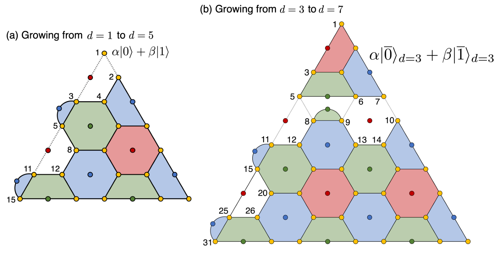
An illustration of the circuit for growing a physical state to a logical state encoded in the triangular color code is given in Fig. 5a. The preparation of in a general distance triangular color code can be done as follows. First, one prepares a stabilizer state (which encodes no logical qubits) that is stabilized by all elements in where is the stabilizer group of a distance triangular color code, is generated by the and -type weight-four operators (white plaquettes) along the boundary of the triangular color code and is generated by the weight-two and -type operators along the boundary (see Fig. 5 for the case where ). The qubit which is in the support of is prepared in the physical state. Note that in the above construction, any of the three boundaries of can be chosen. We chose for convention.
After preparing , the and -type generators of are measured along the boundary . Since the generators of don’t commute with the weight-two generators of , the measurement outcomes of each generator in will be at random. If a outcome is obtained, a Pauli frame update Knill 2005; Terhal 2015; DiVincenzo and Aliferis 2007; Chamberland et al. 2018 needs to be applied to obtain the correct encoded state. In order to perform the correct Pauli frame update based on the random measurement outcomes, we define two one-dimensional graphs and . The vertices of the graph contain the random measurement outcomes of the -type generators in . Each edge corresponds to two qubits which have support on one of the weight-two operators of . Similarly, the vertices of the graph encodes the random measurement outcomes of the -type generators in . An example is provided in Fig. 5 for the triangular color code. Given the set of highlighted vertices of and , Minimum-Weight-Perfect-Matching (MWPM) Edmonds 1965 is applied on both graphs. Each highlighted edge involves performing a weight-two or -type Pauli frame update. For instance, for the graph in Fig. 5b, if the edge is selected during MWPM, the correction is applied to the data. Note that the growing scheme is not fault-tolerant, and thus there is no need to repeat the measurements described above. More details on the implementation of the circuits are provided in Appendix A.
III.2 Performing error correction () using redundant ancilla encoding

In this section we describe the error correction circuits used to detect errors at the output of the circuits. In particular, to guarantee fault-tolerance (see Definition 2 in Appendix B for our definition of fault-tolerance) of our scheme, we require that each circuit is at least a one-flag circuit. For instance, if two faults in two separate -type stabilizers both result in a weight-two data qubit error without any flag qubits flagging, such an error might not be correctable by a triangular color code. Hence such circuits certainly don’t satisfy Definition 2. Note that in Ref. Chamberland et al. 2020b, it was proved that only one flag circuits are required when performing error correction with the triangular color code. The need for only one-flag circuits has to do with the fact that if two-faults occur during a weight-six stabilizer measurement resulting in a weight-three data qubit error, such an error cannot have full support along a minimum-weight logical operator of the triangular color code.
In Fig. 6a we illustrate the full circuit used to measure the stabilizers of a triangular color code along with the CNOT gate scheduling which minimizes the circuit depth for the given qubit layout. The weight-four stabilizers are identical to the ones used in Ref. Chamberland et al. 2020b. However, an important difference can be observed for the weight-six stabilizers, which in addition to using three flag qubits, also uses three ancilla qubits. If an error anti-commutes with a weight-six stabilizer, the measurement outcomes of the three ancillas will have odd parity, otherwise it will have even parity33 3 This is similar to error correction circuits used for Shor error correction Shor 1996; DiVincenzo and Shor 1996. However an important difference is that ancilla verification (i.e. using several ancillas to measure pairs of qubits) is not necessary since the flag qubits ensure that the circuit in Fig. 6b is a two-flag circuit.. The circuit for measuring a weight-six -type stabilizer which respects the CNOT scheduling is given in Fig. 6b. By performing an exhaustive numerical search, we verified that both weight-four and weight-six circuits are two-flag circuits. Since the weights of the stabilizer generators are independent of , having two-flag circuits is sufficient to ensure that the circuits are implemented fault-tolerantly Chamberland and Beverland 2018. Lastly, each weight-four and and weight-six plaquette in a general circuit has the same qubit layout and gate connectivity as those of Fig. 6a.

Now, one might wonder why three ancilla qubits (grey circles of Fig. 6b) instead of a single ancilla are used for measuring the weight-six stabilizers (see for instance the weight-six circuits used in Ref. Chamberland et al. 2020b which only require one ancilla). Indeed, if one is only interested in performing fault-tolerant error correction instead of fault-tolerant quantum computation, then a single ancilla qubit suffices since the additional ancillas don’t provide more information and they also increase the circuit depth. However in Section III.3, we show that to use the same qubit layout for measuring the operator (which is a global operator), the roles of the ancillas and flags in Fig. 6a are reversed. In other words, the ancilla qubits become flag qubits and the flag qubits become ancilla qubits. To ensure that the circuit is a -flag circuit for , we require three flag qubits for every weight-six plaquette and one flag qubit for every weight-four plaquette. Hence if only a single ancilla qubit were used in Fig. 6b, the circuit would not be a three-flag circuit, which would significantly reduce the performance of our protocol (in fact, it would not be possible to achieve the full color code distance for ).
To conclude this section, more ancilla qubits than necessary are used to measure the stabilizer generators of the triangular color code. However using the same qubit layout, the extra ancillas (which become flag qubits when measuring ) ensures that the circuit for measuring the global operator is a -flag circuit (with ) so that at least faults are required to produce a logical failure for the scheme in Fig. 4. We refer to this extra redundancy as redundant ancilla encoding. In Section III.3 we provide explicit circuit constructions to measure .
III.3 -flag circuit construction for the non-destructive measurement of

Here, we describe in detail how to construct a -flag circuit (with ) for the non-destructive measurement of the logical Hadamard operator (i.e., ). The circuits we construct apply to distance triangular color codes with . In Fig. 7a, we present a -flag circuit for measuring of the logical Hadamard operator of the triangular color code. Note that we used the same qubit layout as the one used for the stabilizer measurement circuit ( circuit shown in Fig. 7b) but there is a role reversal between the ancilla qubits (grey circles) and the flag qubits (white circles). That is, the ancilla qubits in the stabilizer measurement circuit are used as flag qubits in the logical Hadamard measurement circuit and vice versa.
We now explain why the circuit in Fig. 7a performs a non-destructive measurement of the logical Hadamard operator . Note that the ancilla qubits (grey circles) in Fig. 7a are prepared in the logical plus state of the -qubit repetition code (or the -qubit GHZ state ) through the CNOT gates between the ancilla qubits (see Fig. 8a). Then, as shown in Fig. 8b, the controlled-Hadamard gates implement a logical controlled-Hadamard gate between the ancilla -qubit repetition code and the data color code. Eventually, the ancilla qubits (in the -qubit repetition code) are measured in the logical X basis via a measurement (see Fig. 8d). Hence, the circuits in Figs. 8a, b, and d implement the simple non-destructive Hadamard measurement circuit in Fig. 2a, except that the ancilla qubits are now encoded in the -qubit repetition code and the data qubits are encoded in the triangular color code.
The most important element of the logical Hadamard measurement circuit in Fig. 7 is the parity check of the ancilla GHZ state by using flag qubits (see Fig. 8c). Note that the flag qubits (white circles) non-destructively measure the parity of the ancilla GHZ state , , and , or the three stabilizers of the -qubit repetition code (we labeled the qubits from the top to the bottom and from the left to the right). These stabilizer measurements will be trivial if all the CNOT gates in Fig. 8a are perfect. However, CNOT gate failures can result in non-trivial flag measurement outcomes. In particular, there are several single CNOT gate failure events that can cause a data qubit error of weight- or higher. For the Hadamard circuit to be -flag, all these failure events should be caught by flag qubits. Indeed, we verify via a comprehensive numerical search that the logical Hadamard circuit in Fig. 7a is a -flag circuit by confirming that if there is a single fault at any location resulting in a data qubit error with , at least one flag qubit flags.

Similarly, we construct a -flag circuit for the logical Hadamard measurement of the triangular color code and a -flag circuit for the triangular color code (see Fig. 9). The design principle is essentially the same. That is, in the case (i.e., ), we first generate a -qubit GHZ state in the ancilla qubits (grey circles), or equivalently, a logical plus state of the -qubit repetition code. The entangled ancilla qubits are then coupled to all of the data qubits (yellow circles) through controlled-Hadamard gates. Finally, the ancilla qubits (in the -qubit repetition code) are measured in the the logical X basis via a measurement. Thus, the circuit in Fig. 9a implements a non-destructive measurement of the logical Hadamard measurement of the color code by using ancilla qubits in the -qubit repetition code.
Precisely because the ancilla qubits are encoded in the -qubit repetition code, we can check if the ancilla qubits are reliably prepared in the logical plus state by measuring (out of ) stabilizers of the ancilla -qubit repetition code using flag qubits (white circles). Performing an exhaustive numerical search, we can confirm that the circuit is a -flag circuit. A -flag circuit for the logical Hadamard measurement of the triangular color code is constructed in the same way by using ancilla qubits prepared in the logical plus state of the -qubit repetition code, and using flag qubits checking the (out of ) stabilizers of the -qubit repetition code (see Fig. 9b). We point out that the order and time steps at which the CNOT gates, used to measure the stabilizers of the repetition code with flag qubits, are implemented is very important and must be carefully chosen.
Recall that we used a redundant ancilla encoding scheme in the stabilizer measurement circuits (see Fig. 6). Specifically, we redundantly used three ancilla qubits to measure the weight- stabilizers of the triangular color code. Note that these ancilla qubits are used as flag qubits in the logical Hadamard measurement circuits with . Thus, the redundant ancilla encoding in the stabilizer measurement circuits allows the logical Hadamard measurement circuits to have sufficiently many flag qubits while maintaining the same two-dimensional qubit layout. In particular, the logical Hadamard measurement circuits and have and flag qubits that check (out of ) and (out of ) stabilizers of the ancilla GHZ state, respectively. Without the redundant ancilla encoding, we would have had flag qubits in the case and flag qubits in the case, as opposed to and flag qubits, respectively. We remark that the logical Hadamard measurement circuits and that are constructed with such fewer flag qubits are not -flag and -flag circuits. Thus, the redundant ancilla encoding scheme plays a crucial role in guaranteeing the desired fault-tolerance property of the logical Hadamard measurement circuits.
IV Resource overhead for preparing encoded states with physical Clifford gates
| (physical Clifford’s) | |||||
| 17 | 16 | 594 | |||
| 68 | 55 | 5,694 | |||
| 231 | 118 | 27,431 | |||
| 17 | 16 | 611 | |||
| 84 | 55 | 7,010 | |||
| 449 | 118 | 53,359 | |||
| 18 | 16 | 630 | |||
| 103 | 55 | 8,648 | |||
| 870 | 118 | 103,500 | |||
| 18 | 16 | 650 | |||
| 127 | 55 | 10,656 | |||
| 1,700 | 118 | 202,268 | |||
| 19 | 16 | 670 | |||
| 156 | 55 | 13,115 | |||
| 3,312 | 118 | 394,177 |
In this section we provide the logical failure rates of the states prepared using the scheme presented in Section III and the noise model described in Section II.2. We also provide the average number of qubits required to produce such states.
Since the entire sequence of operations in Fig. 4 fault-tolerantly prepares for , for a physical error rate (see the description of the circuit-level noise model used in Section II.2), the output state is afflicted by a logical fault with probability
| (12) |
where counts all the combinations of faults which lead to acceptance of our scheme while resulting in a logical , or error. Hence
| (13) |
where is the total number of locations which can fail in the combined circuits of Fig. 4. Note that Eq. 13 is a strict inequality since there are a lot of benign locations in the circuits used to prepare . For values of , the higher order terms in Eq. 12 were found to have a negligible impact on .

Given the acceptance probability for preparing a distance encoded state with physical error rate , the average number of qubits is given by
| (14) |
where is the number of data qubits, and is the total number of ancilla and flag qubits used in the circuits and . Since each weight-six stabilizer generator requires six qubits, and each weight-four stabilizer three qubits, we have
| (15) |
where and are the number of weight-four and weight-six stabilizers. Putting everything together, we obtain
| (16) |
Note that if we repeat the protocol for preparing until the output state is accepted (at the expense of having a higher time cost), the number of qubits required to prepare is simply
| (17) |
We now consider the space-time overhead for implementing the scheme in Section III where additional qubits (as in Eq. 16) are used to minimize the time cost. In particular, the space-time overhead is given as
| (18) |
where and are the total number of time steps required to implement one round of the circuits and respectively. The factor of 14 in Eq. 18 comes from the 14 times steps required to implement the circuit . Note that we pessimistically assume that all time steps are reached when implementing the circuits in Fig. 4. This is pessimistic since when the magic state preparation scheme does not pass the verification steps, fewer than time steps are used.
It is important to point out that due to the presence of gates (which are non-Clifford) used to implement the controlled-Hadamard gates (see Fig. 2b), an efficient Monte-Carlo simulation of the circuits using Gottesman-Knill error propagation Gottesman 1999; Aaronson and Gottesman 2004 is not possible. Consequently, we divided the Monte-Carlo simulation to calculate and into two parts. First, we perform a Monte-Carlo simulation of the circuit used to prepare . If the output error has a non-trivial syndrome or is a logical operator, the protocol of Section III is aborted, otherwise, we proceed to simulate the and circuits. We define to be the probability of proceeding to the and circuits. Note that there could be other faults in the and circuits that would cause the protocol to be accepted even though had a non-trivial syndrome or was a logical operator. However such an event would require at least faults, and since the large majority of malignant error locations are found in and , such an approximation only affects in Eq. 12 by a small constant factor.
Now, to simulate the circuit , we use the fact that and . Hence if an or error is input to a or gate, we pessimistically apply an or error to the output, each with probability. Such an approximation would be exact if twirling operations were performed both before and after the and gates (see Appendix C). To be clear, we do not propose applying twirling operations when implementing our scheme as this could reduce the performance. The approximations stated here are performed to allow us to simulate our scheme on a classical computer.
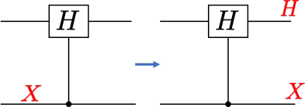
We also note that an error propagating through the control qubit of a controlled-Hadamard gate results in a Hadamard error applied to the data (see Fig. 10). Therefore, an error on the first CNOT between the ancillas and in the circuit implementing results in the error (which acts trivially on ) without any flag qubits flagging (see Fig. 11 for an illustration). However, since the controlled-Hadamard is decomposed as in Fig. 2b, an error on the control qubit of the controlled- gate results in a error on the data. Therefore, if we propagate (arising from the error at the CNOT mentioned above) through the gates as described above, the output will not be a benign error. As such, prior to the application of the gates, let be the component of the data qubit errors. For instance, if the data qubit errors are , then . The component which is propagated through the gates is chosen to be . This prevents a single fault from causing a logical error without any flag qubits flagging in our simulations.
If all flag qubit and ancilla qubit measurement outcomes in the applications of the and circuits are trivial, the output state is accepted. We define to be the probability of acceptance for the second part of the simulation (i.e. the simulation of the and circuits) . Hence the total acceptance probability is . To determine if the output error of an accepted state is correctable, we perform one round of perfect error correction using the the Lift decoder.

The values of , , and for are given in Table 1 and were obtained by performing Monte-Carlo simulations on AWS clusters. For values of resulting in very low logical failure rates, extrapolation of the best fit curve (using Eq. 12) was used to compute the logical error rate of . Note that using the version of the protocol in Section III, an state can be prepared with logical failure rate with using only 68 qubits on average when . Alternatively, one may use qubits and repeat the protocol until it is accepted (with an acceptance probability ). Further, one can use the version of the protocol to produce an state with logical failure rate with only 231 qubits on average. Similarly as above, one may use qubits and repeat the protocol until it is accepted (with an acceptance probability ). In comparison, when , the non fault-tolerant magic state distillation scheme in Ref. Litinski 2019 requires 810 and 1150 qubits to prepare magic states with failure rates and , respectively. We note that recent works suggests that is the appropriate regime to have small enough decoding hardware requirements Delfosse 2020.
An important remark is that the space-time overhead values obtained in Ref. Litinski 2019 cannot directly be compared with those of Table 1. Roughly speaking, one would need to multiply the numbers obtained in Ref. Litinski 2019 by at least (where the factor of 6 comes from the fact that 6 time steps are required to measure all the surface code stabilizers). To be clear, Eq. 18 takes into account the total number of time steps required for each measurement cycle. As such, our scheme provides a space-time overhead improvement, say to obtain a magic state with , by at least an order of magnitude. One of the main reasons for the reduction in overhead is that we did not need to use encoded Clifford operations due to the fault-tolerant properties of our circuits. In Ref. Litinski 2019, the magic state being distilled needed to be encoded in the surface code (so that the logical error rates of the encoded Clifford gates are approximately ) to obtain an output state with failure probability . On the other hand, our scheme does not require encoded Clifford gates with very low error rates, and instead works with physical Clifford gates with an error rate .
(a) (b)
(b)
V Preparing with encoded stabilizer operations
In Section IV we showed that using physical Clifford operations which fail with probability , states with logical error rates near and can be prepared with 68 and 231 qubits on average. However, for many quantum algorithms, states with even lower logical error rates are required. This can be accomplished by encoding all stabilizer operations in a triangular color code since such encoded operations have much lower error rates compared to physical unencoded stabilizer operations. We now describe the implementation of our preparation scheme presented in Section III with encoded stabilizer operations. In what follows, we denote as the state produced when implementing the scheme of Section III with encoded stabilizer operations. Further, the circuits , and will be denoted as , and when implemented with encoded stabilizer operations (see Fig. 12).
Suppose that in order to prepare an state with some target logical error rate, we require all stabilizer operations to be encoded in a triangular color code of distance . First, states are prepared using the scheme described in Section III (with and with physical stabilizer operations). The distance is chosen such that the states have smaller logical failure rates compared with those of the distance encoded stabilizer operations. The states are used to implement the logical gates (see Fig. 1) and for injection in the circuit . If , the states must first be grown into states using a technique analogous to the one illustrated in Fig. 13. The circuits performing such growing operations are denoted since all operations are implemented with physical gates. Using encoded states ensures that stabilizer operations encoded in a distance triangular color code can be used with the prepared magic states.
The circuits are implemented as follows. As in Section III.1, a stabilizer state is prepared, and operators supported on the white plaquettes seperating and are measured (this step can be viewed as gauge fixing of an underlying subsystem code Vuillot et al. 2019a). Measurements of all operators supported on each plaquette of the distance triangular color code are repeated times to correct errors and to distinguish measurement errors from the random outcomes obtained when measuring the white plaquettes. An example for implementing is provided in Fig. 13.
Once enough states have been prepared (see below), such states are injected into the circuits of Fig. 1 to perform the logical gates, in addition to being injected in the circuit (see for instance the circuit used in Fig. 5, but with distance encoded stabilizer operations). The final state used for computation is then prepared repeating the same steps as in Section III (i.e. applying pairs of the and circuits) with each stabilizer operation encoded in the distance triangular color code. In Fig. 12 we provide a schematic illustration of the full scheme described above.
To compute the overhead for preparing the state , we consider the case where all the gates are simultaneously implemented during the second time step of the circuit. We can thus prepare states which are used for implementing the gates in addition to injecting one of these states into the circuit . The probability that at least states pass the verification test is given by
| (19) |
where is the probability of acceptance for preparing the state . An accepted state then grows into an encoded state since the Clifford operations are chosen to be encoded in the distance triangular color code. Since the weight-six stabilizers of the stabilizer state (and all encoded Clifford gates) are obtained from the circuit in Fig. 14, the total number of qubits required for the stabilizer state is
| (20) |
and the number of qubits for each state is
| (21) |
Lastly, since the qubits in the implementation for preparing using the protocol of Section III are encoded in the triangular color code with distance , we require an additional
| (22) |
qubits. Hence, the total average number of qubits required to prepare is
| (23) |
where is the acceptance probability for preparing with Clifford operations encoded in a distance triangular color code. For a fixed value of , is chosen to minimize Eq. 23. Note that we assume that all the qubits used to prepare the states can be reused to implement the gates at the end of the circuit. In doing so, it is assumed that the time scale required to prepare the states is less than or equal to the time scale required to implemented all the encoded operations prior to applying the gates at the end of the circuit. Also, the denominator of Eq. 23 has the factor for the following reasons: In the first time step, an extra magic state is used in the circuit (see Fig. 12). Second, only states are required when implementing the sequence of gates (which are implemented after the gates). The term is taken to the power of since the circuit is repeated times (and each circuit requires the injection of magic states for both the and gates).
If one is willing to significantly increase the time-overhead required for preparing all the magic states used in the preparation scheme of , the number of qubits required to prepare can be reduced compared to the requirements given by Eq. 23. In particular, one can repeat the protocol until magic states are simultaneously accepted and ready to be grown to states. Such qubits are then reused to prepare states prior to implementing the and gates every time the circuit is repeated. If any of the states do not pass the verification test described in Section III, the protocol is aborted. In this case, the minimum number of qubits required to prepare is simply
| (24) |
We now describe how to compute the space-time overhead for preparing . We first need to consider the space-time overhead of preparing the states, and then growing them to states. The space-time overhead for preparing a single state is obtain in a similar way to Eq. 18 and is given by
| (25) |
where and correspond to the number of time steps for implementing the and circuits. When growing a state to , the measurements of the plaquettes are repeated times, with the maximum number of time steps for each round of measurement being (which come from measuring the stabilizers for the state using the circuits of Fig. 6). Therefore, the space-time overhead for growing an to state is given by
| (26) |
Since we prepare such states, the space-time overhead for preparing all of the states which are injected in the gates and the circuit is
| (27) |
The last step consists of implementing the pairs of and circuits. Each implementation of an encoded Clifford gate requires rounds of error correction, and an encoded block consists of qubits. Furthermore, if , the total number of time steps for one round of error correction is 16. Thus the space-time overhead for preparing with encoded Clifford gates is
| (28) |
Note that in Eq. 28, we choose a large enough time window for the implementation of the circuits , and to ensure that at least time steps occur allowing one to decode to the full color code distance. Since all logical gates in this time window are Clifford (for , this is true for gates applied in between the and gates) and performed using lattice surgery Horsman et al. 2012; Landahl and Ryan-Anderson 2014; Litinski and Oppen 2018; G. Fowler and Gidney 2018, one can perform the appropriate Pauli frame updates to incorporate the correct decoding scheme over the full triangular color code cycle. In our numerical simulations, we pessimistically added an error at each logical Clifford gate location using the failure probabilities obtained in Ref. Chamberland et al. 2020b instead of using such probabilities for adding failures over a full distance triangular color code cycle. Hence the values reported in Table 2 are upper bounds on the exact values that would be obtained using our scheme.
| Color code distance () | |||||||
| 10,917 | 6,288 | ||||||
| 14,955 | 12,795 | ||||||
| 25,265 | 19,320 | ||||||
| 53,449 | 36,420 | ||||||
| 16,262 | 15,600 | ||||||
| 28,141 | 26,364 | ||||||
| 43,329 | 39,936 | ||||||
| 62,540 | 56,316 | ||||||
| 84,200 | 75,504 |
| Surface code distance () | ||||||
| 10,025 | 9,506 | |||||
| 60,886 | 47,324 |
In Table 2 we provide the average number of qubits, minimum number of qubits and space-time overhead required to prepare states with logical failure rates . To obtain such results, we assume that each Clifford gate encoded in the triangular color code fails according to the logical error rate polynomials obtained in Ref. Chamberland et al. 2020b (which we call ). Hence, when preparing the stabilizer state and for all encoded Clifford operations, the ancilla qubit layout for the weight-six checks are chosen as in Fig. 14 (note that the weight-four checks remain unchanged). Further, the distance is chosen to be the smallest which ensures that has a lower logical error rate than . Lastly, due to the low failure rates of the encoded components, to obtain we repeat the simulation described in Section IV for physical values of , and extrapolate the best fit curves to the regime where .
The numerical values obtained in Table 2 shows that the least costly scheme to prepare the state with when is to first prepare the states with , and to grow these states to encoded states. Using distance encoded stabilizer operations, the final magic state is prepared using the distance scheme of Section III. On average, the amount of qubits required to prepare such a state is 10,917 and the space-time overhead is . If the time cost for preparing the states is of a lesser concern, the minimum number of qubits required to prepare with is 6,288. To compare with other schemes, in Ref. Litinski 2019, a magic state with a logical error failure rate of required a minimum of 16,400 qubits.
To obtain a state with when using a small amount of resources requires encoded stabilizer operations with much lower logical failure rates than what is achieved with the triangular color code family. One viable option is to use stabilizer operations encoded in the surface code due to the low error rates that can be achieved when Fowler et al. 2012b. However, in such a setting, after the states have been prepared, they must be teleported to the surface code before they can be injected in the circuit of Fig. 1 and in the circuit implementing . In particular, one can convert the color code encoded state to the surface code using lattice surgery techniques as was done in Ref. Nautrup et al. 2017. In Table 3 we provide estimates of the qubit overhead for preparing when the stabilizer operations are encoded in the surface code. The cost of first encoding the states in the color code and then using extra qubits to convert such states into the surface code is taken into account. However, we assume that the quality of the encoded states does not change when performing lattice surgery. Although such an omission is optimistic, we verified numerically that when only the and gate locations are allowed to fail, the protocol of Section III produces states with logical error rates two to four orders of magnitude (depending on the value of ) less than when all stabilizer operations fail according to the noise model described in Section II.2. As such, the simulation provides evidence that the logical error rates obtained in Table 3 are good estimates of the error rates that would be obtained when considering errors introduced when performing lattice surgery to obtain surface code encoded states.
Instead of performing lattice surgery to convert a color code encoded state to one encoded in the surface code, another option would be to initially prepare an encoded state in a small distance surface code using some other method, such as a magic state distillation protocol. The states would then be injected in the gate circuits of Fig. 1 in addition to the circuit in order to prepare an state using the methods presented in Section III. To obtain comparable logical failure rates to the ones shown in Table 2 (say ) at , the surface code distance would need to be if the scheme was chosen, if the scheme was chosen and if the scheme were chosen. Note that the logical error rate of the surface code is given by for , for , and for Fowler et al. 2012b. In contrast, would be required if conventional non fault-tolerant magic state distillation schemes are used, since in this case the stabilizer operations should have a logical error rate as low as . A careful analysis of the overhead would require choosing the appropriate magic state distillation protocol (or some other scheme which uses fault-tolerant circuits to prepare encoded magic states) and therefore such an analysis is left for future work.
Lastly, one could also directly prepare an encoded state in a distance surface code using the non-fault-tolerant state injection methods of Ref. Li 2015. Such states would then be injected in the scheme for preparing (see Fig. 12) with encoded stabilizer operations in a distance surface code. In this case, the injected states would have much higher failure rates compared to the encoded stabilizer operations. In such a setting, extending our scheme to could potentially be very beneficial. However, to avoid preparing a state with , one could consider a two level approach. As a first step, one could inject states to first prepare an state with . Afterwords, the obtained could be further injected to prepare a new state with .
VI Conclusion and outlook
In this work we showed how to prepare an -type magic state in a fault-tolerant way using a two-dimensional color code architecture requiring only nearest-neighbor interactions. The proposed architecture can be used to both measure local stabilizers of the color code in addition to a global operator, without the need for changing the qubit layout. Such an architecture was made possible with the use of flag qubits, in addition to a new concept which we call redundant ancilla encoding. Estimating the performance of our scheme, we showed that when , only 68 and 231 qubits are required to prepare an encoded state with logical error rates and respectively. In addition, we also showed how our scheme can be used with encoded stabilizer operations to achieve significantly lower logical failure rates, both in the regime where and . We stress that our results were obtained by considering a full circuit-level depolarizing noise model, where all stabilizer operations could fail.
We also point out key differences between magic state distillation schemes and our fault-tolerant methods for preparing magic states. Magic state distillation is a top-down approach, where error detection circuits are designed to prepare magic states without regard to their fault-tolerant properties. It is assumed that appropriate code distances for the encoded Clifford operations will be chosen to ensure that consecutive rounds of distillation will produce higher fidelity magic states. Our scheme, which uses flag-qubits and redundant ancilla encoding, is a bottom-up approach. The fault-tolerant properties of the magic state preparation circuits are prioritized and emphasis is given towards constructing -flag circuits for large . As such, to obtain magic states with very low failure rates, if encoded stabilizer operations are required, such operations can fail with error rates commensurate to the magic states being injected.
The underlying codes that are used for our work belong to the triangular color code family. One avenue of exploration would be to consider the 4.8.8 color code family (see for instance Refs. Landahl et al. 2011; Kesselring et al. 2018) for potentially better performance. In addition, the color codes used to encode the Clifford operations required two and three ancillas for the weight-four and weight-six stabilizers respectively. Using similar edge weight renormalization schemes to those described in Ref. Chamberland et al. 2020b, one could use fewer ancillas for measuring each stabilizer while maintaining the full effective code distance of the Lift decoder. Due to the smaller number of fault locations and reduced ancilla requirements, such an implementation could potentially significantly reduce the overhead for preparing encoded states.
When considering the implementation of our scheme with encoded stabilizer operations using the surface code, the version of our scheme was optimal for both and . A clear direction of future work would be to find a -flag circuit (with ) allowing a fault-tolerant implementation of a scheme. Such a scheme could potentially further reduce the overhead for preparing states with very low error rates.
The schemes considered in this work to prepare states are error detection schemes. In particular, for and , the acceptance probability for preparing an state is very low (for instance, only when ). One way to improve the acceptance probability could be to use qubits encoded in a bosonic code Albert et al. 2018 (such as a GKP code Gottesman et al. 2001) and concatenate such qubits with the color code (the GKP code concatenated with the surface code was considered in Refs. Fukui et al. 2018; Vuillot et al. 2019b; Noh and Chamberland 2020 for quantum memories). By using bosonic qubits, repeated rounds of error correction at the bosonic level prior to measuring the logical Hadamard operator and stabilizers of the color code could be performed to reduce some of the errors afflicting the data and ancilla qubits. Another possibility would be to develop an error correction scheme for preparing an state which applies directly to the color code family. Such a scheme would have higher logical error rates compared to an error detection scheme, and the scheduling of the controlled-Hadamard gates would have to be considered more carefully. However, since an error correction scheme would not require any post selection, there could be an interval of physical error rates where it achieved better performance compared to the error detection scheme considered in this work.
With a plethora of possible research directions for preparing magic states in a fault-tolerant way which build upon our work, and given the realistic hardware constraints that are built directly into our schemes, we believe our work paves the way for achieving very low overhead universal quantum computation with both near-term and long-term quantum devices.
Acknowledgments
C.C. acknowledges Yihe Tang and Milan Cvitkovic for their help in setting up the computing resources with the AWS clusters which were used for performing all the numerical simulations in this work. We would like to thank Earl Campbell, Aleksander Kubica and Fernando Brandao for useful discussions. We thank Simone Severini, Bill Vass and Dominique L’Eplattenier for their guidance and help with submitting the paper. We also thank Kevin Dothager for his help with IP.
Appendix A Non fault-tolerant state preparation scheme
In this section, we show how measuring the white plaquettes when implementing the growing schemes in Figs. 5 and 13 and applying the corrections from the matching graphs results in the correct encoded state. Let us first consider the growing scheme shown in Fig. 15a that converts a physical input state into a logical state encoded in the distance- triangular color code. In this scheme, we first prepare a stabilizer state that is stabilized by out of the stabilizer generators of the distance- triangular color code
| (30) |
as well as the following four weight-2 stabilizers
| (31) |
We define to be the group generated by the operators in Eqs. 30 and 31. Note that can be prepared by first preparing all qubits in the state, and then measuring only the -type generators in . As such, we have
| (32) |
One can readily check that is stabilized by all the stabilizers in Eqs. 30 and 31 as desired.
Once is prepared, we measure the four missing stabilizer generators of the distance- triangular code given by
| (33) |
Such operators are the white plaquettes shown in Fig. 15a. We define to the group generated by the operators in Eq. 33.
Initially, the system is in the state
| (34) |
After measuring the -type stabilizers of , we get the following state
| (35) |
conditioned on obtaining where when measuring and . In any case, we can always convert the state to by applying a correction operator
| (36) |
since anti-commutes with and , and anti-commutes with . Note that the correction operators in Eq. 36 can be determined by implementing MWPM on the matching graph shown in Fig. 5b. Thus after the correction, we are always left with the state
| (37) |
where we used .
Next, we measure the two -type stabilizers of . After the measurement, the state becomes
| (38) |
conditioned on the measurement outcomes . Performing the same steps as above, the state can be converted to by applying an appropriate correction operator which is determined by implementing MWPM on the matching graph shown in Fig. 5b. Afterwords, we are left with
| (39) |
where is the logical zero state of the distance triangular color code. Note that
| (40) |
Since is the logical X operator of the distance- triangular color code, we can conclude that the output state is given by
| (41) |
Hence, the output state is the is the desired state encoded in the triangular color code.
We now move on to the growing scheme shown in Fig. 15b that converts an input state (encoded in the triangular color code) into a logical state encoded in the triangular color code. As in the previous scheme, we first prepare a stabilizer state that is stabilized by out of the generators of the triangular color code as well as weight- stabilizers which are given by
| (42) |
To initiate the growing scheme, we measure the following stabilizers of the triangular color code, which are represented by the white plaquettes of Fig. 15b
| (43) |
Note that the operators in Eq. 43 are not stabilizers of the stabilizer state and the triangular color code (which is being merged with ).
Once the stabilizer state is prepared, and prior to measuring the operators in Eq. 43, the system is in the state
| (44) |
After measuring the three -type stabilizers in Eq. 43, we get the following state
| (45) |
where the values of depend on the measurement outcomes of , and . As in the case where a physical state was grown to an encoded state of the triangular color code, we can convert any output state to by applying a correction operator
| (46) |
Note that correction operators of Eq. 46 can be determined by implementing MWPM on the matching graph shown in Fig. 13b. After the applying such corrections, we are always left with the state
| (47) |
The final step consists of measuring the three -type stabilizers in Eq. 43. The state in Eq. 47 then becomes
| (48) |
where the values of depend on the measurement outcomes of , and . The states can be mapped to the state again by applying an appropriate correction operator as was done in Eq. 46, but with -type operators. Thus, at the end of the growing scheme, we have
| (49) |
Repeating a similar analysis as in Eq. 40, we get the following desired result
| (50) |
Appendix B Proof of fault-tolerance for the state preparation scheme in Section III.
In this section we show that in order for the magic state preparation protocol of Section III to be fault-tolerant, the pair of and circuits need to be repeated a minimum of times. In what follows, we say that a state preparation protocol is -fault-tolerant if the following two conditions are satisfied (see for instance Refs.Gottesman 2010; Chamberland and Cross 2019):
Definition 2.
Fault-tolerant state preparation
For , a state-preparation protocol using a distance- stabilizer code is -fault-tolerant if the following two conditions are satisfied:
- 1.
If there are faults during the state-preparation protocol with , the resulting state differs from a codeword by an error of at most weight .
- 2.
If there are faults during the state-preparation protocol with , then ideally decoding the output state results in the same state that would be obtained from the fault-free state-preparation scheme.
Here ideally decoding refers to performing a round of fault-free error correction. In what follows, the code belongs to the triangular color code family. Further, since the circuits are valid for , the following arguments apply for code distances of the triangular color code that are no greater than seven.
We have already verified numerically that the and circuits are -flag circuits (with ). Hence if there are faults in the or circuits resulting in an error with either or (for any of the stabilizers ), at least one flag qubit will flag and the protocol aborts.

First, we consider all the possible output errors of the fault-free implementation of the circuits given an input error (see Fig. 16). The input error arises from faults which occur during the implementation of the circuit (see for instance Figs. 4 and 5). We illustrate all possible cases for and for each case we show the resulting output errors. Note that in what follows, the state (where is the number of ancilla qubits) can be replaced by the single-qubit state without changing the final result. We also write the controlled-Hadamard gate as . Lastly, given an error , will correspond to the error syndrome of obtained by measuring all the stabilizer generators of the underlying stabilizer code used to encode the data.
Case 1: or .
Suppose . Prior to performing the gate, we have
| (51) |
Applying the gate and using the identity , transforms to which is given by
| (52) |
Similarly, if , performing the same steps shows that
| (53) |
From Eqs. 52 and 53, we see that performing the -basis measurement and discarding the ancilla, the final output state is if a outcome is obtained (which is the desired state), and if a outcome is obtained (each occurring with a probability).
Case 2: .
Prior to performing the gate, we have
| (54) |
Applying the gate and using the identity , we have
| (55) |
Hence the ancilla measurement outcome will always be with the final output state .
Case 3: .
In this case, we assume that where 0 is the all zeros bit string of length (where is the number of data qubits of the underlying stabilizer code encoding the data). Further, we define . Performing an analogous calculation to the one leading to Eq. 55, we have
| (56) |
Hence, if the ancilla is measured as , the output state will be whereas a outcome will yield . Both measurement outcomes occur with probability. Further, note that and are detectable errors.
Case 4: or .
Again, we assume that . Performing the same calculations as above, we find
| (57) |
Again, the ancilla measurement outcomes will be , each occurring with probability. A outcome yields the output state and a outcome yields . In both cases, the errors afflicting the state will be detected by a fault-free circuit. The case where yields identical output states, up to a global sign. We will now explain why the and circuits need to come in pairs.
In the example provided leading to Eq. 57, if the measurement outcome is obtained, there can be an fault resulting in the error at the very beginning of the subsequent circuit cancelling the term multiplying and thus resulting in the error . As such, there is a chance that a trivial syndrome is obtained when implementing the circuit, resulting in the output error . However, by applying the circuit a second time (assuming it is fault-free), Case 1 shows that a outcome cannot result in an output state with a logical fault. Since the pair of and circuits are repeated times, at least one such pair must be fault-free if the total number of faults has . This example illustrates the importance of applying the and circuits in pairs. For instance, if all the circuits were repeated times, followed by the repetition of the circuits times, an error of the form would always result in a outcome of the circuits and the output error would be unchanged. Then as shown above, a single fault at the beginning of the first circuit could result in a trivial syndrome with probability (with an output error ) and all subsequent rounds of syndrome measurement would yield the trivial syndrome.

Now suppose there are faults spread throughout all the circuits illustrated in Fig. 4. We consider the worst case scenario, where a single fault results in an error (which should be detected by our protocol), and the remaining faults all result in measurement errors (and such faults can potentially add additional data qubit errors, say if it arises from a CNOT gate) preventing from being detected in either the or circuits. Since the pair of and circuits are repeated times, at least one pair of and circuits will be fault-free and thus not afflicted by measurement errors. From the above, if the and circuits are fault-free, then measurement outcomes in both circuits cannot yield an uncorrectable output error. Further, since all the and circuits are -flag circuits (with ), the final output error must have and as such, it must be a correctable error.
We note that in the general case, where a state is used instead of the state, we can replace and measurement outcomes with even and odd parity measurement outcomes, and the same conclusions would follow.
Appendix C Twirling approximation
In this section, we show that a non-Pauli error after a or gate can be converted via a noise twirling operation into an incoherent mixture of Pauli errors. To be clear, we do not propose to physically perform the noise twirling after the and gates as part of the protocol as this can reduce the performance of our scheme. Instead, we aim to show that the approximations we performed in our numerical simulations are justified.
Suppose for instance there is an input error to a gate. Recall that the input Pauli error is converted through the gate into a non-Pauli error . We make this non-Pauli error into an incoherent mixture of Pauli errors by applying and before and after the noisy gate where the rotation angle is drawn uniformly from the range . Note that
| (58) |
where we used the fact that commutes with for any . Then, since
| (59) |
we have
| (60) |
and thus
| (61) |
That is, the output Hadamard error is converted via the noise twirling to an incoherent mixture of the Pauli and errors, each with probability (see Fig. 17). The same reasoning holds for any output error for any . On the other hand, since a Pauli error commutes with the gate and the gates, it is unaffected by the noise twirling and remains to be a Pauli error.
References
- Eastin and Knill [2009] Bryan Eastin and Emanuel Knill. Restrictions on transversal encoded quantum gate sets. Phys. Rev. Lett., 102:110502, Mar 2009. doi:10.1103/PhysRevLett.102.110502. URL https://link.aps.org/doi/10.1103/PhysRevLett.102.110502.
- Knill et al. [1996] Emanuel Knill, Raymond Laflamme, and Wojciech H. Zurek. Threshold accuracy for quantum computation. arXiv: quant-ph/9610011, 1996.
- Paetznick and Reichardt [2013] Adam Paetznick and Ben W. Reichardt. Universal fault-tolerant quantum computation with only transversal gates and error correction. Phys. Rev. Lett., 111:090505, Aug 2013. doi:10.1103/PhysRevLett.111.090505. URL https://link.aps.org/doi/10.1103/PhysRevLett.111.090505.
- Jochym-O’Connor and Laflamme [2014] Tomas Jochym-O’Connor and Raymond Laflamme. Using concatenated quantum codes for universal fault-tolerant quantum gates. Phys. Rev. Lett., 112:010505, 2014. doi:10.1103/PhysRevLett.112.010505. URL http://link.aps.org/doi/10.1103/PhysRevLett.112.010505.
- Anderson et al. [2014] Jonas T. Anderson, Guillaume Duclos-Cianci, and David Poulin. Phys. Rev. Lett., 113:080501, Aug 2014. doi:10.1103/PhysRevLett.113.080501. URL https://link.aps.org/doi/10.1103/PhysRevLett.113.080501.
- Bombín [2015] Héctor Bombín. Gauge color codes: optimal transversal gates and gauge fixing in topological stabilizer codes. New J. Phys., 17(8):083002, 2015. URL https://iopscience.iop.org/article/10.1088/1367-2630/17/8/083002/meta.
- Bravyi and Cross [2015] Sergey Bravyi and Andrew Cross. Doubled Color Codes. arXiv e-prints, art. arXiv:1509.03239, Sep 2015. URL https://arxiv.org/abs/1509.03239.
- Jochym-O’Connor and Bartlett [2016] Tomas Jochym-O’Connor and Stephen D. Bartlett. Stacked codes: Universal fault-tolerant quantum computation in a two-dimensional layout. Phys. Rev. A, 93:022323, 2016. doi:10.1103/PhysRevA.93.022323. URL http://link.aps.org/doi/10.1103/PhysRevA.93.022323.
- Yoder et al. [2016] Theodore J. Yoder, Ryuji Takagi, and Isaac L. Chuang. Universal fault-tolerant gates on concatenated stabilizer codes. Phys. Rev. X, 6:031039, Sep 2016. doi:10.1103/PhysRevX.6.031039. URL https://link.aps.org/doi/10.1103/PhysRevX.6.031039.
- Chamberland et al. [2016] Christopher Chamberland, Tomas Jochym-O’Connor, and Raymond Laflamme. Thresholds for universal concatenated quantum codes. Phys. Rev. Lett., 117:010501, Jun 2016. doi:10.1103/PhysRevLett.117.010501. URL https://link.aps.org/doi/10.1103/PhysRevLett.117.010501.
- Chamberland et al. [2017] Christopher Chamberland, Tomas Jochym-O’Connor, and Raymond Laflamme. Overhead analysis of universal concatenated quantum codes. Phys. Rev. A, 95:022313, Feb 2017. doi:10.1103/PhysRevA.95.022313. URL https://link.aps.org/doi/10.1103/PhysRevA.95.022313.
- Chamberland and Jochym-O’Connor [2017] Christopher Chamberland and Tomas Jochym-O’Connor. Error suppression via complementary gauge choices in reed-muller codes. Quantum Science and Technology, 2(3):035008, 2017. URL http://stacks.iop.org/2058-9565/2/i=3/a=035008.
- Chamberland and Cross [2019] Christopher Chamberland and Andrew W. Cross. Fault-tolerant magic state preparation with flag qubits. Quantum, 3:143, May 2019. ISSN 2521-327X. doi:10.22331/q-2019-05-20-143. URL https://doi.org/10.22331/q-2019-05-20-143.
- Jochym-O’Connor [2019] Tomas Jochym-O’Connor. Fault-tolerant gates via homological product codes. Quantum, 3:120, February 2019. ISSN 2521-327X. doi:10.22331/q-2019-02-04-120. URL https://doi.org/10.22331/q-2019-02-04-120.
- Lavasani et al. [2019] Ali Lavasani, Guanyu Zhu, and Maissam Barkeshli. Universal logical gates with constant overhead: instantaneous Dehn twists for hyperbolic quantum codes. Quantum, 3:180, August 2019. ISSN 2521-327X. doi:10.22331/q-2019-08-26-180. URL https://doi.org/10.22331/q-2019-08-26-180.
- Bravyi and Kitaev [2005] Sergey Bravyi and Alexei Kitaev. Universal quantum computation with ideal clifford gates and noisy ancillas. Phys. Rev. A, 71:022316, Feb 2005. doi:10.1103/PhysRevA.71.022316. URL https://link.aps.org/doi/10.1103/PhysRevA.71.022316.
- Reichardt [2005] Ben W. Reichardt. Quantum universality from magic states distillation applied to css codes. Quantum Information Processing, 4(3):251–264, Aug 2005. ISSN 1573-1332. doi:10.1007/s11128-005-7654-8. URL https://doi.org/10.1007/s11128-005-7654-8.
- Meier et al. [2013] Adam M. Meier, Bryan Eastin, and Emanuel Knill. Magic-state distillation with the four-qubit code. Quantum Info. Comput., 13(3-4):0195–0209, 2013.
- Bravyi and Haah [2012] Sergey Bravyi and Jeongwan Haah. Magic-state distillation with low overhead. Phys. Rev. A, 86:052329, Nov 2012. doi:10.1103/PhysRevA.86.052329. URL https://link.aps.org/doi/10.1103/PhysRevA.86.052329.
- Fowler et al. [2013] Austin G. Fowler, Simon J. Devitt, and Cody Jones. Surface code implementation of block code state distillation. Scientific Reports, (3):1939, 2013. doi:10.1038/srep01939.
- O’Gorman and Campbell [2017] Joe O’Gorman and Earl T. Campbell. Quantum computation with realistic magic-state factories. Phys. Rev. A, 95:032338, Mar 2017. doi:10.1103/PhysRevA.95.032338. URL https://link.aps.org/doi/10.1103/PhysRevA.95.032338.
- Haah et al. [2017] Jeongwan Haah, Matthew B. Hastings, D. Poulin, and D. Wecker. Magic state distillation with low space overhead and optimal asymptotic input count. Quantum, 1:31, October 2017. ISSN 2521-327X. doi:10.22331/q-2017-10-03-31. URL https://doi.org/10.22331/q-2017-10-03-31.
- Haah et al. [2018] Jeongwan Haah, Matthew B. Hastings, David Poulin, and Dave Wecker. Magic state distillation at intermediate size. Quantum Info. Comput., 18(1):97–165, 2018. ISSN 0114-0140.
- Hastings and Haah [2018] Matthew B. Hastings and Jeongwan Haah. Distillation with sublogarithmic overhead. Phys. Rev. Lett., 120:050504, Jan 2018. doi:10.1103/PhysRevLett.120.050504. URL https://link.aps.org/doi/10.1103/PhysRevLett.120.050504.
- Haah and Hastings [2018] Jeongwan Haah and Matthew B. Hastings. Codes and Protocols for Distilling , controlled-, and Toffoli Gates. Quantum, 2:71, June 2018. ISSN 2521-327X. doi:10.22331/q-2018-06-07-71. URL https://doi.org/10.22331/q-2018-06-07-71.
- Litinski [2019] Daniel Litinski. Magic State Distillation: Not as Costly as You Think. Quantum, 3:205, December 2019. ISSN 2521-327X. doi:10.22331/q-2019-12-02-205. URL https://doi.org/10.22331/q-2019-12-02-205.
- Yoder and Kim [2017] Theodore J. Yoder and Isaac H. Kim. The surface code with a twist. Quantum, 1:2, April 2017. ISSN 2521-327X. doi:10.22331/q-2017-04-25-2. URL https://doi.org/10.22331/q-2017-04-25-2.
- Chao and Reichardt [2018a] Rui Chao and Ben W. Reichardt. Quantum error correction with only two extra qubits. Phys. Rev. Lett., 121:050502, Aug 2018a. doi:10.1103/PhysRevLett.121.050502. URL https://link.aps.org/doi/10.1103/PhysRevLett.121.050502.
- Chao and Reichardt [2018b] Rui Chao and Ben W. Reichardt. Fault-tolerant quantum computation with few qubits. npj Quantum Information, 4(1):42, 2018b. doi:10.1038/s41534-018-0085-z. URL https://doi.org/10.1038/s41534-018-0085-z.
- Chamberland and Beverland [2018] Christopher Chamberland and Michael E. Beverland. Flag fault-tolerant error correction with arbitrary distance codes. Quantum, 2:53, February 2018. ISSN 2521-327X. doi:10.22331/q-2018-02-08-53. URL https://doi.org/10.22331/q-2018-02-08-53.
- Tansuwannont et al. [2020] Theerapat Tansuwannont, Christopher Chamberland, and Debbie Leung. Flag fault-tolerant error correction, measurement, and quantum computation for cyclic calderbank-shor-steane codes. Phys. Rev. A, 101:012342, Jan 2020. doi:10.1103/PhysRevA.101.012342. URL https://link.aps.org/doi/10.1103/PhysRevA.101.012342.
- Reichardt [2018] Ben W. Reichardt. Fault-tolerant quantum error correction for steane’s seven-qubit color code with few or no extra qubits. arXiv:quant-ph/1804.06995, 2018. URL https://arxiv.org/abs/1804.06995.
- Shi et al. [2019] Yunong Shi, Christopher Chamberland, and Andrew Cross. Fault-tolerant preparation of approximate GKP states. New Journal of Physics, 21(9):093007, sep 2019. doi:10.1088/1367-2630/ab3a62. URL https://doi.org/10.1088%2F1367-2630%2Fab3a62.
- Chamberland et al. [2020a] Christopher Chamberland, Guanyu Zhu, Theodore J. Yoder, Jared B. Hertzberg, and Andrew W. Cross. Topological and subsystem codes on low-degree graphs with flag qubits. Phys. Rev. X, 10:011022, Jan 2020a. doi:10.1103/PhysRevX.10.011022. URL https://link.aps.org/doi/10.1103/PhysRevX.10.011022.
- Chao and Reichardt [2019] Rui Chao and Ben W. Reichardt. Flag fault-tolerant error correction for any stabilizer code. arXiv e-prints, art. arXiv:1912.09549, Dec 2019.
- Chamberland et al. [2020b] Christopher Chamberland, Aleksander Kubica, Theodore J Yoder, and Guanyu Zhu. Triangular color codes on trivalent graphs with flag qubits. New Journal of Physics, 22(2):023019, feb 2020b. doi:10.1088/1367-2630/ab68fd. URL https://doi.org/10.1088%2F1367-2630%2Fab68fd.
- Bombin and Martin-Delgado [2006] H. Bombin and M. A. Martin-Delgado. Topological quantum distillation. Phys. Rev. Lett., 97:180501, Oct 2006. doi:10.1103/PhysRevLett.97.180501. URL https://link.aps.org/doi/10.1103/PhysRevLett.97.180501.
- Kubica and Beverland [2015] Aleksander Kubica and Michael E. Beverland. Universal transversal gates with color codes: A simplified approach. Phys. Rev. A, 91:032330, 2015. doi:10.1103/PhysRevA.91.032330. URL http://link.aps.org/doi/10.1103/PhysRevA.91.032330.
- Kubica [2018] Aleksander Kubica. The ABCs of the color code: A study of topological quantum codes as toy models for fault-tolerant quantum computation and quantum phases of matter. PhD thesis, 2018. URL https://thesis.library.caltech.edu/10955/.
- Kubica and Delfosse [2019] Aleksander Kubica and Nicolas Delfosse. Efficient color code decoders in dimensions from toric code decoders. arXiv e-prints, art. arXiv:1905.07393, May 2019. URL https://arxiv.org/abs/1905.07393.
- Kitaev [1997] Alexei Y. Kitaev. Quantum computations: algorithms and error correction. Russian Mathematical Surveys, 52(6):1191–1249, 1997.
- Dawson and Nielsen [2006] Christopher M. Dawson and Michael Nielsen. The solovay-kitaev algorithm. Quant. Inf. Comput., 6:81–95, 2006.
- Fowler et al. [2012a] Austin G. Fowler, Matteo Mariantoni, John M. Martinis, and Andrew N. Cleland. Surface codes: Towards practical large-scale quantum computation. Phys. Rev. A, 86:032324, Sep 2012a. doi:10.1103/PhysRevA.86.032324. URL https://link.aps.org/doi/10.1103/PhysRevA.86.032324.
- Kivlichan et al. [2019] Ian D. Kivlichan, Craig Gidney, Dominic W. Berry, Nathan Wiebe, Jarrod McClean, Wei Sun, Zhang Jiang, Nicholas Rubin, Austin Fowler, Alán Aspuru-Guzik, Hartmut Neven, and Ryan Babbush. Improved Fault-Tolerant Quantum Simulation of Condensed-Phase Correlated Electrons via Trotterization. arXiv e-prints, art. arXiv:1902.10673, Feb 2019. URL https://arxiv.org/abs/1902.10673.
- Gidney and Ekerå [2019] Craig Gidney and Martin Ekerå. How to factor 2048 bit RSA integers in 8 hours using 20 million noisy qubits. arXiv e-prints, art. arXiv:1905.09749, May 2019. URL https://arxiv.org/abs/1905.09749.
- Aliferis et al. [2006] Panos Aliferis, Daniel Gottesman, and John Preskill. Quantum accuracy threshold for concatenated distance-3 codes. Quantum Info. Comput., 6(2):97–165, March 2006. ISSN 1533-7146. URL http://dl.acm.org/citation.cfm?id=2011665.2011666.
- Knill [2005] Emanuel Knill. Quantum computing with realistically noisy devices. Nature, 434(7029):39–44, 2005. doi:10.1038/nature03350. URL https://www.nature.com/articles/nature03350.
- Terhal [2015] Barbara M. Terhal. Quantum error correction for quantum memories. Rev. Mod. Phys., 87:307–346, Apr 2015. doi:10.1103/RevModPhys.87.307. URL https://link.aps.org/doi/10.1103/RevModPhys.87.307.
- DiVincenzo and Aliferis [2007] David P. DiVincenzo and Panos Aliferis. Effective fault-tolerant quantum computation with slow measurements. Phys. Rev. Lett., 98:020501, Jan 2007. doi:10.1103/PhysRevLett.98.020501. URL https://link.aps.org/doi/10.1103/PhysRevLett.98.020501.
- Chamberland et al. [2018] Christopher Chamberland, Pavithran Iyer, and David Poulin. Fault-Tolerant Quantum Computing in the Pauli or Clifford Frame with Slow Error Diagnostics. Quantum, 2:43, January 2018. ISSN 2521-327X. doi:10.22331/q-2018-01-04-43. URL https://doi.org/10.22331/q-2018-01-04-43.
- Edmonds [1965] Jack Edmonds. Paths, trees, and flowers. Canadian Journal of mathematics, 17(3):449–467, 1965. doi:10.4153/CJM-1965-045-4. URL https://www.cambridge.org/core/journals/canadian-journal-of-mathematics/article/paths-trees-and-flowers/08B492B72322C4130AE800C0610E0E21.
- Shor [1996] Peter W. Shor. Fault-tolerant quantum computation. Proceedings., 37th Annual Symposium on Foundations of Computer Science, pages 56–65, 1996. URL http://dl.acm.org/citation.cfm?id=874062.875509.
- DiVincenzo and Shor [1996] David P. DiVincenzo and Peter W. Shor. Fault-tolerant error correction with efficient quantum codes. Phys. Rev. Lett., 77:3260–3263, Oct 1996. doi:10.1103/PhysRevLett.77.3260. URL https://link.aps.org/doi/10.1103/PhysRevLett.77.3260.
- Gottesman [1999] Daniel Gottesman. The Heisenberg representation of quantum computers. Proceedings, XXII International Colloquium on Group Theoretical Methods in Physics, pages 32–43, 1999.
- Aaronson and Gottesman [2004] Scott Aaronson and Daniel Gottesman. Improved simulation of stabilizer circuits. Phys. Rev. A, 70:052328, Nov 2004. doi:10.1103/PhysRevA.70.052328. URL https://link.aps.org/doi/10.1103/PhysRevA.70.052328.
- Delfosse [2020] Nicolas Delfosse. Hierarchical decoding to reduce hardware requirements for quantum computing. arXiv e-prints, art. arXiv:2001.11427, January 2020. URL https://arxiv.org/abs/2001.11427.
- Vuillot et al. [2019a] Christophe Vuillot, Lingling Lao, Ben Criger, Carmen García Almudéver, Koen Bertels, and Barbara M Terhal. Code deformation and lattice surgery are gauge fixing. New Journal of Physics, 21(3):033028, mar 2019a. doi:10.1088/1367-2630/ab0199. URL https://doi.org/10.1088%2F1367-2630%2Fab0199.
- Horsman et al. [2012] Clare Horsman, Austin G Fowler, Simon Devitt, and Rodney Van Meter. Surface code quantum computing by lattice surgery. New Journal of Physics, 14(12):123011, dec 2012. doi:10.1088/1367-2630/14/12/123011. URL https://doi.org/10.1088%2F1367-2630%2F14%2F12%2F123011.
- Landahl and Ryan-Anderson [2014] Andrew J. Landahl and Ciaran Ryan-Anderson. Quantum computing by color-code lattice surgery. arXiv e-prints, art. arXiv:1407.5103, Jul 2014. URL https://arxiv.org/abs/1407.5103.
- Litinski and Oppen [2018] Daniel Litinski and Felix von Oppen. Lattice Surgery with a Twist: Simplifying Clifford Gates of Surface Codes. Quantum, 2:62, May 2018. ISSN 2521-327X. doi:10.22331/q-2018-05-04-62. URL https://doi.org/10.22331/q-2018-05-04-62.
- G. Fowler and Gidney [2018] Austin G. Fowler and Craig Gidney. Low overhead quantum computation using lattice surgery. arXiv:1808.06709, 2018.
- Nautrup et al. [2017] Hendrik Poulsen Nautrup, Nicolai Friis, and Hans J. Briegel. Fault-tolerant interface between quantum memories and quantum processors. Nature Communications, 8:1321, NOV 2017. doi:10.1038/s41467-017-01418-2. URL https://doi.org/10.1038/s41467-017-01418-2.
- Fowler et al. [2012b] Austin G. Fowler, Adam C. Whiteside, Angus L. McInnes, and Alimohammad Rabbani. Topological code autotune. Phys. Rev. X, 2:041003, Oct 2012b. doi:10.1103/PhysRevX.2.041003. URL https://link.aps.org/doi/10.1103/PhysRevX.2.041003.
- Li [2015] Ying Li. A magic state’s fidelity can be superior to the operations that created it. New Journal of Physics, 17(2):023037, feb 2015. doi:10.1088/1367-2630/17/2/023037. URL https://doi.org/10.1088%2F1367-2630%2F17%2F2%2F023037.
- Landahl et al. [2011] Andrew J. Landahl, Jonas T. Anderson, and Patrick R. Rice. Fault-tolerant quantum computing with color codes. arXiv:1108.5738, 2011. URL https://arxiv.org/abs/1108.5738.
- Kesselring et al. [2018] Markus S. Kesselring, Fernando Pastawski, Jens Eisert, and Benjamin J. Brown. The boundaries and twist defects of the color code and their applications to topological quantum computation. Quantum, 2:101, October 2018. ISSN 2521-327X. doi:10.22331/q-2018-10-19-101. URL https://doi.org/10.22331/q-2018-10-19-101.
- Albert et al. [2018] Victor V. Albert, Kyungjoo Noh, Kasper Duivenvoorden, Dylan J. Young, R. T. Brierley, Philip Reinhold, Christophe Vuillot, Linshu Li, Chao Shen, S. M. Girvin, Barbara M. Terhal, and Liang Jiang. Performance and structure of single-mode bosonic codes. Phys. Rev. A, 97:032346, Mar 2018. doi:10.1103/PhysRevA.97.032346. URL https://link.aps.org/doi/10.1103/PhysRevA.97.032346.
- Gottesman et al. [2001] Daniel Gottesman, Alexei Kitaev, and John Preskill. Encoding a qubit in an oscillator. Phys. Rev. A, 64:012310, Jun 2001. doi:10.1103/PhysRevA.64.012310. URL https://link.aps.org/doi/10.1103/PhysRevA.64.012310.
- Fukui et al. [2018] Kosuke Fukui, Akihisa Tomita, Atsushi Okamoto, and Keisuke Fujii. High-threshold fault-tolerant quantum computation with analog quantum error correction. Phys. Rev. X, 8:021054, May 2018. doi:10.1103/PhysRevX.8.021054. URL https://link.aps.org/doi/10.1103/PhysRevX.8.021054.
- Vuillot et al. [2019b] Christophe Vuillot, Hamed Asasi, Yang Wang, Leonid P. Pryadko, and Barbara M. Terhal. Quantum error correction with the toric gottesman-kitaev-preskill code. Phys. Rev. A, 99:032344, Mar 2019b. doi:10.1103/PhysRevA.99.032344. URL https://link.aps.org/doi/10.1103/PhysRevA.99.032344.
- Noh and Chamberland [2020] Kyungjoo Noh and Christopher Chamberland. Fault-tolerant bosonic quantum error correction with the surface–gottesman-kitaev-preskill code. Phys. Rev. A, 101:012316, Jan 2020. doi:10.1103/PhysRevA.101.012316. URL https://link.aps.org/doi/10.1103/PhysRevA.101.012316.
- Gottesman [2010] Daniel Gottesman. An introduction to quantum error correction and fault-tolerant quantum computation. Proceedings of Symposia in Applied Mathematics, 68:13–58, 2010. URL https://arxiv.org/abs/0904.2557.