Membranes for spontaneous separation of pedestrian counter flowsPreprint: Submitted to Physical Review **
Abstract
Designing efficient traffic lanes for pedestrians is a critical aspect of urban planning as walking remains the most common form of mobility among the increasingly diverse methods of transportation. Herein, we investigate pedestrian counter flows in a straight corridor, in which two groups of people are walking in opposite directions. We demonstrate, using a molecular dynamics approach applying the social force model, that a simple array of obstacles improves flow rates by producing flow separations even in crowded situations. We also report on a developed model describing the separation behavior that regards an array of obstacles as a membrane and induces spontaneous separation of pedestrians groups. When appropriately designed, those obstacles are fully capable of controlling the filtering direction so that pedestrians tend to keep moving to their left (or right) spontaneously. These results have the potential to provide useful guidelines for industrial designs aimed at improving ubiquitous human mobility.
I Introduction
Modern transportation systems are becoming increasingly complex and often require different time and spatial scales, as represented by the rapid growth of the diverse transportation methods and mobility technologies Barbosa et al. 2018; Barthelemy 2019. Since there are still numerous phenomena that are not fully understood within each of such transportation systems, both experimental and theoretical studies aimed at understanding such phenomena have been performed continuously Lv et al. 2014; Varga et al. 2016. Among the different transportation methods, walking remains the most fundamental, so pedestrian flows have been widely studied Scott 1974; Polus et al. 1983; Gipps and Marksjö 1985; Virkler and Elayadath 1994. In typical experimental studies, pedestrian trajectories are observed and analyzed by recording their motions with video cameras or using laser measurements Seyfried et al. 2005; Helbing et al. 2007; Johansson et al. 2008; Chattaraj et al. 2009; Moussaïd et al. 2009; Zanlungo et al. 2011; Zhang et al. 2011; Zhang et al. 2012. On the other hand, theoretical approaches have also been used to gain a systematic understanding of observed pedestrian behaviors and/or for predicting the pedestrian flows under various circumstances Helbing 1992; Burstedde et al. 2001; Bonabeau 2002; Hughes 2002; Seyfried et al. 2006. For example, the so-called social force model, first proposed by Helbing and Molnár Helbing and Molnár 1995, is one of the most widely used theoretical approaches used to model pedestrian movements, which enables us to simulate flows using molecular dynamics Helbing et al. 2000a; Lakoba et al. 2005; Oliveira et al. 2016; Sticco et al. 2017; Kang et al. 2019.
In the present study, we also employ the social force model to investigate pedestrian behaviors in a straight corridor in which two groups of people are walking in opposite directions. Similar situations with two groups of particles moving in the other directions have been extensively studied in the context of lane and pattern formations not only of pedestrians Ikeda and Kim 2017; Feliciani et al. 2018 but also of various physical particles, such as charged colloids Vissers et al. 2011a; Vissers et al. 2011b; Tarama et al. 2019, microswimmers Kogler and Klapp 2015, and plasmas Sütterlin et al. 2009; Sarma et al. 2020. These studies are focused mainly on a bulk system without obstacles.Here we demonstrate that separation-membrane-like obstacles placed along the centerline of a corridor improve flow efficiency even in crowded situations. This is because the presence of those obstacles triggers a spontaneous separation of the pedestrians groups, thereby resulting in an unconscious “keep-left” pedestrian mentality, as illustrated in Fig. 1. Although relevant studies have been reported, such as effects of placing columns asymmetrically near an exit Helbing et al. 2000a; Shiwakoti et al. 2019, and a partition line effect controlling the critical density in the jamming transition Takimoto et al. 2002, the enhancement of a pedestrian counter flow by means of particular choices of obstacles is, to our knowledge, new. We also report on the development of a model describing the separation behavior, which is inspired by a reminiscent membrane separating multi-component fluids. These findings related to pedestrian group filtering could potentially provide useful guidelines for improving daily pedestrian flows.
II Problem
Here we consider a throng of pedestrians walking in a straight corridor of width and length , as shown in Fig. 2(a). In this context, out of pedestrians are walking in the direction, and the remaining pedestrians are traveling in the direction. Here, we assume . We also assume that the periodic boundary condition in the direction, which is set so that the global average density of , is constant. Such situations, in which a self-organizing lane-formation and clogging phenomenon occurs at high-density points (which is often called jamming-transition), have been extensively studied Helbing et al. 2000b; Nagatani 2009; Zhang et al. 2012; Feliciani and Nishinari 2016; Feliciani et al. 2018.
According to the experiments examining the impacts of congestion in a corridor, pedestrian flow velocities tend to decrease as density increases (see, e.g., Ref. Zhang et al. 2012 and Fig. S1 in the Supplemental Information (SI)). In the present study, we consider situations in which an obstacle array is placed along the median line of a corridor to suppress velocity reductions and to control pedestrian flow patterns. To be more specific, we consider elliptic obstacles with major and minor axes of lengths and , respectively, which are placed on the median line of the corridor () at intervals of . The obstacles are commonly angled, such that the angle between the axis and the major axis is .
III Molecular dynamics simulation
Before showing simulation results, we will first summarize the model equations used in the molecular dynamics. Each pedestrian is modeled by a spherical particle, the dynamics of which is governed by the following equation of motion:
| (1) |
where , , and are the mass, radius, and velocity of the th particle, respectively. The first term on the right-hand side represents the force driving the pedestrian in the desired direction with velocity and relaxation time . The second term is the sum of the pairwise interaction force between pedestrian particles and . In the third term, the walls and obstacles are expressed in terms of groups of fixed particles, indexed by wall, with being the interaction force between particle and those fixed particles (see Fig. S2 in the SI). Finally, indicates the Gaussian white noise satisfying , , where is the Kronecker delta, is the identity matrix, and is the noise intensity parameter.
The explicit form of is given by
| (2) |
where , , , and are the model parameters, and , with being the distance between particle and , and is the Heaviside function, the value of which is unity for and zero otherwise. The normal unit vector is pointing from the position of particle to that of , and the unit vector is in the tangential direction perpendicular to . is the projection of the relative velocity between and on . The interaction force has the same form as Eq. (2) with the parameters and simply replaced by and .
All the simulations are implemented using the open source code LAMMPS lam. The source codes in the original package are modified to incorporate the pairwise interactions corresponding to Eq. (2) (see Sec. S1 of the SI for details). The specific values of parameters used in our simulations are summarized as shown below. The mass of each pedestrian is kg and the diameter of a pedestrian is m. We choose m as the diameter of fixed particles. The model parameters for the pairwise interaction force given in Eq. (2) are fixed at N, m, N/m, Pas, and s, following Ref. Helbing et al. 2000a. The repulsive force is taken into account only for m, and is otherwise cut off. The value of pedestrians’ desired velocity or terminal velocity is set as m/s, which is based on the experimental result in Ref. Zhang et al. 2012, and the noise intensity is chosen as N2 to reproduce the experimental density-velocity relationship discussed below (see Fig. S3 in the SI). The initial configuration is constructed with randomly distributed pedestrians, and each simulation runs over steps with time step s. Note that the simulations set with these parameters reproduce the experimental results well, as shown in Fig. S1 in the SI. In the following simulation results, the geometrical parameters are fixed at m, m, m, m, and m unless otherwise stated.
We show in Fig. 2(b) the fundamental diagram, namely the density-velocity relation for our system. More precisely, we plot the velocity averaged over the pedestrians walking in the direction versus the average density (). Here, and in what follows, the time average is taken over steps for each run, and no fewer than five runs with different initial configurations are used to obtain each averaged quantity. In general, pedestrian counter flows under ordinary situations in the absence of obstacles exhibit congestion as density increases, resulting in monotonically decreasing velocity (see, e.g., Ref. Zhang et al. 2012). This feature is properly captured by our simulation for the no-obstacle case results, which are shown as a reference in Fig. 2(b). In the same figure, the case in the presence of obstacles with , i.e., the symmetric obstacles, which have no impact on this fundamental diagram, is also shown. On the other hand, the corridor with emplaced asymmetric obstacles ( and ) maintains a much higher velocity than that in the previous two cases. The simulation snapshots (see Fig. S4 in the SI) imply that this significant velocity enhancement (thus, flux) is a result of lane formations that reduce friction between particles passing in opposite directions. We also note here that the formed lanes are stable. In other words, once a lane is formed, it tends to occupy the same side of the corridor for a long time. In our simulations, the lanes with emplaced asymmetric obstacles do not change sides during the simulation runs (see Fig. S5 in the SI). At this point, we see that the flow structure, i.e., whether or not lanes are formed, plays an essential role in improving traffic flow efficiency.
Next, we investigate the structure of the pedestrian counter flows in the presence of the obstacles in greater detail. In order to quantify the flow structure discussed above, we introduce the order parameter , which is defined as
| (3) |
where and are the component of the velocity and the component of the position of particle , respectively Oliveira et al. 2016. Since is the median line of the corridor, the value of is positive when particle moves in the direction in the region . Therefore, when most pedestrians keep to their left, and similarly if they keep to their right. The value of vanishes when the pedestrians walking in the opposite directions are uniformly distributed or when the keep-left and keep-right patterns appear with equal probability. This order parameter is normalized such that when the pedestrian flow is perfectly separated into two streams (see Fig. 1).
In Fig. 3(a), we show the order parameter as a function of the average density for the situations considered in Fig. 2(b), supplemented by the cases of and . In the absence of obstacles, the system is purely symmetric about . Hence, we see in the entire range of . Again, the symmetric obstacles with do not influence the flow structure. On the other hand, when the obstacles are angled by , for the wide range up to m-2, and is larger than even for the high densities. In the case of shallower angles, the absolute value of is smaller, but remains significant. In other words, the pedestrian flow exhibits clear self-organization by separating into two groups that keep to their left or to their right as they travel in opposite directions.
In view of the fact that the separation does not occur in the absence of obstacles, the lane formation obtained here is in contrast to that observed in a bulk situation, i.e., in a system without obstacles, for certain parameter ranges (see, e.g., Ikeda and Kim 2017; Glanz and Löwen 2012; Ikeda et al. 2012; Reichhardt et al. 2018). In the present case, the asymmetry of obstacles is the main contribution to the lane formation and stabilization. This is confirmed by the symmetric obstacle results, which still do not lead to the stable lane formation. The local interaction with a tilted obstacle transfers a part of momentum in the direction into a momentum in the direction. Depending on the direction (along ) from which a particle collides, the gained momentum in the direction in fact differs. This local imbalance diffuses to the entire region of the corridor, which results in the complete separation with observed in Fig. 3(a).
In order to examine the effect of the geometrical parameter in greater detail, we show the relationship between and at several values of in Fig. 3(b). The order parameter sign is determined by the angle , such that for and for , which confirms that tuning the geometrical parameter enables us not only to induce self-organized lane formations but also to control the flow patterns precisely, i.e., keep them left or keep them right. Figure 3(b) also shows that the control sensitivity to depends on the density. More specifically, is rather sensitive for the high density value of m-2, whereas it is robust for the lower density value of m-2.

IV Membrane model for separation
We next present a model reproducing the separation behavior of the pedestrian counter flows discussed above. We begin with noting that the role played by the obstacles is reminiscent of the effects of filtering membranes used to separate different fluid components. Therefore, inspired by the modeling of such filtering membranes Marbach and Bocquet 2017; Marbach and Bocquet 2019, we now construct a differential equation describing the dynamics of pedestrian concentrations. For simplicity, we assume that the pedestrian density and velocity values are uniform on each side of the membrane. The density of pedestrians walking in the or direction in the region is written as . Then, the density in the region is because the density of people going in each direction in the whole area of is . Furthermore, assuming the density of all pedestrians is uniformly distributed, we have . Hence, the system density distribution is fully determined once a governing equation for is solved. In the following, is simply written as , and the order parameter is expressed as .
Using the same idea as the model describing concentration variations between two reservoirs separated by a membrane Zwanzig 1990; Marbach and Bocquet 2017, we model the behavior of as follows:
| (4) |
where, is the thickness of the membrane, is the area of interest (now the region ). In contrast to the models describing ordinary membranes Zwanzig 1990; Marbach and Bocquet 2017, the equation above contains two terms driving the density change characterized by and ;the parameter controls the driving force that mixes the pedestrians such that the values of in and approach. On the other hand, is the parameter for the driving force that separates the pedestrians moving in the and directions such that approaches . The solution of Eq. (5) is readily obtained as , where and are the constants determined from the initial conditions and is the stationary solution.
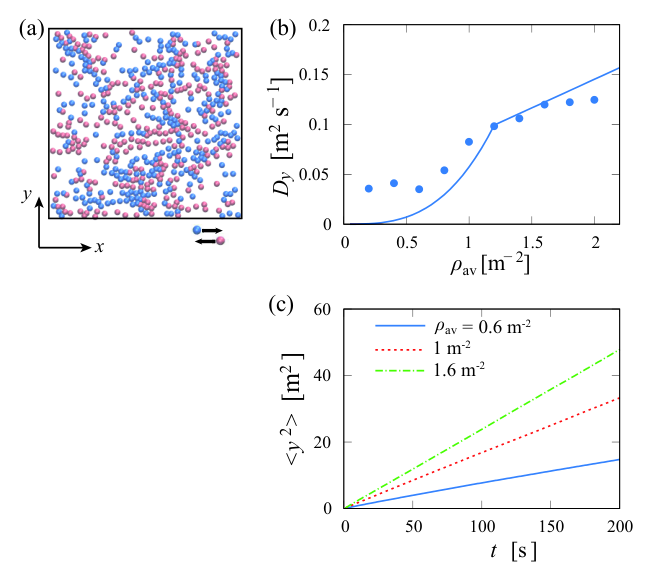
Diffusion phenomena should dominate the physical mechanisms of mixing. Since the analysis of counter flows in the bulk region shows generally increasing diffusion coefficient with increasing density, we assume a functional form for which increases with density. The diffusion coefficient in the direction obtained under wall-free bulk conditions, in comparison with our model for , is found in Fig. S6 of the SI, where the linear time dependent of the mean square displacement shows the ordinary diffusion process in the direction.On the other hand, in modeling the separating force , we take into account the fact that a certain separation effect is observed even in the low-density region. Hence we assume a constant value for with respect to . However, since the separation ability should depend on the the geometrical details of the obstacles forming the membrane, we assume that depends on the angle . We note that a common function of is assigned to for all the results shown below (see Fig. S7 in the SI,) of which the functional form reflects the shape of obstacles constituting the membrane. The values of obtained from the steady solution of Eq. (5) are shown in Figs. 3(a) and (b). The results of molecular dynamics simulations, including the variation of decreasing in Fig. 3(a), are well captured. In addition, the molecular dynamics results examining the effect of the interval between obstacles are well predicted by the present model with the same parameter set (see Fig. S8 in the SI).
From the above comparison, we conclude that the minimum model given in Eq. (5), based on the membrane dynamics (with the driving forces chosen appropriately), is capable of predicting the spontaneous separation effect of the pedestrian flow. In addition to the steady-state behavior focused on in the above discussion, the present model was also examined for transient response, and its consistency with the molecular dynamics simulations was confirmed to be within the parameter range where the approximation of Eq. (5) is valid. In other words, situations where the corridor area is not too wide and the density to each side of the membrane varies uniformly. More specifically, for the molecular dynamics simulation, we measure the relaxation time taken to reach the steady-state exhibiting , starting from the initial condition with , in which the pedestrians traveling in both directions distribute uniformly in the whole corridor. These results are then compared with the corresponding relaxation time predicted by the model given in Eq. (5). The resulting model predictions agree well with the molecular dynamics results under conditions in which is not too large (see Fig. S9 in the SI).
V Conclusion
To summarize, we have shown that simple asymmetric obstacles emplaced in a corridor enable us to control pedestrian flow patterns by inducing self-organizing lane formations. As demonstrated in Fig. 2, the structured pedestrian flows are more efficient than those of ordinary unstructured crowds. Thus, the present results could contribute to developing new concepts for engineering corridor designs in ways that create efficient traffic lanes. Here, the asymmetry is generated by designing the geometrical shape of obstacles. However, this is merely an example for realizing the spontaneous separation of pedestrians. The original concept of the “social force” employed in our molecular dynamics simulations includes psychological interactions forces acting effectively on the pedestrians. Therefore, designing psychological obstacles, constructed by means of visual effects such as photo-regulation, electronic signage, or some other methods, could provide alternative approaches, and will be included among our future research topics.
Our membrane model for separation has shown good agreements with the molecular dynamics simulation results, as shown in Fig. 3. This is an example of the analogies found in multidisciplinary studies, in which a theory established for microscopic physics is used to explain macroscopic phenomena at a length scale that is orders of magnitude higher than the original micro-scale. We believe that our finding suggests a way forward for the field of mobility and transportation, particularly when viewed in tandem with ideas on various unobvious phenomena present in microscopic transportation systems.
Acknowledgments
The authors would like to thank Dr. K. Kidono of Toyota Central R&D Labs., Inc. and M. Shimada of the University of Tokyo for the useful discussions.
References
- Barbosa et al. (2018) Hugo Barbosa, Marc Barthelemy, Gourab Ghoshal, Charlotte R James, Maxime Lenormand, Thomas Louail, Ronaldo Menezes, José J Ramasco, Filippo Simini, and Marcello Tomasini, “Human mobility: Models and applications,” Phys. Rep. 734, 1–74 (2018).
- Barthelemy (2019) Marc Barthelemy, “The statistical physics of cities,” Nature Rev. Phys. , 1 (2019).
- Lv et al. (2014) Yisheng Lv, Yanjie Duan, Wenwen Kang, Zhengxi Li, and Fei-Yue Wang, “Traffic flow prediction with big data: a deep learning approach,” IEEE T. Intell. Transp. 16, 865–873 (2014).
- Varga et al. (2016) Levente Varga, András Kovács, Geza Tóth, István Papp, and Zoltán Néda, “Further we travel the faster we go,” PloS One 11, e0148913 (2016).
- Scott (1974) Allen J Scott, “A theoretical model of pedestrian flow,” Socio-Econ. Plan. Sci. 8, 317–322 (1974).
- Polus et al. (1983) Abishai Polus, Joseph L Schofer, and Ariela Ushpiz, “Pedestrian flow and level of service,” J. Transp. Eng. 109, 46–56 (1983).
- Gipps and Marksjö (1985) Peter G Gipps and B Marksjö, “A micro-simulation model for pedestrian flows,” Math. Comput. Simulat. 27, 95–105 (1985).
- Virkler and Elayadath (1994) Mark R Virkler and Sathish Elayadath, “Pedestrian speed-flow-density relationships,” Transp. Res. Rec. 1438, 51–18 (1994).
- Seyfried et al. (2005) Armin Seyfried, Bernhard Steffen, Wolfram Klingsch, and Maik Boltes, “The fundamental diagram of pedestrian movement revisited,” J. Stat. Mech. 2005, P10002 (2005).
- Helbing et al. (2007) Dirk Helbing, Anders Johansson, and Habib Zein Al-Abideen, “Dynamics of crowd disasters: An empirical study,” Phys. Rev. E 75, 046109 (2007).
- Johansson et al. (2008) Anders Johansson, Dirk Helbing, Habib Z Al-Abideen, and Salim Al-Bosta, “From crowd dynamics to crowd safety: a video-based analysis,” Adv. Complex Sys. 11, 497–527 (2008).
- Chattaraj et al. (2009) Ujjal Chattaraj, Armin Seyfried, and Partha Chakroborty, “Comparison of pedestrian fundamental diagram across cultures,” Adv. Complex Sys. 12, 393–405 (2009).
- Moussaïd et al. (2009) Mehdi Moussaïd, Dirk Helbing, Simon Garnier, Anders Johansson, Maud Combe, and Guy Theraulaz, “Experimental study of the behavioural mechanisms underlying self-organization in human crowds,” Proc. R. Soc. Lond. B 276, 2755–2762 (2009).
- Zanlungo et al. (2011) Francesco Zanlungo, Tetsushi Ikeda, and Takayuki Kanda, “Social force model with explicit collision prediction,” Europhys. Lett. 93, 68005 (2011).
- Zhang et al. (2011) Jun Zhang, Wolfram Klingsch, Andreas Schadschneider, and Armin Seyfried, “Transitions in pedestrian fundamental diagrams of straight corridors and T-junctions,” J. Stat. Mech. Theory E. 2011, P06004 (2011).
- Zhang et al. (2012) Jun Zhang, Wolfram Klingsch, Andreas Schadschneider, and Armin Seyfried, “Ordering in bidirectional pedestrian flows and its influence on the fundamental diagram,” J. Stat. Mech. Theory E. 2012, P02002 (2012).
- Helbing (1992) Dirk Helbing, “A fluid dynamic model for the movement of pedestrians,” Complex Systems 6, 391–415 (1992).
- Burstedde et al. (2001) Carsten Burstedde, Kai Klauck, Andreas Schadschneider, and Johannes Zittartz, “Simulation of pedestrian dynamics using a two-dimensional cellular automaton,” Physica A 295, 507–525 (2001).
- Bonabeau (2002) Eric Bonabeau, “Agent-based modeling: Methods and techniques for simulating human systems,” Proc. Natl. Acad. Sci. 99, 7280–7287 (2002).
- Hughes (2002) Roger L Hughes, “A continuum theory for the flow of pedestrians,” Transport Res. B-Meth 36, 507–535 (2002).
- Seyfried et al. (2006) Armin Seyfried, Bernhard Steffen, and Thomas Lippert, “Basics of modelling the pedestrian flow,” Physica A 368, 232–238 (2006).
- Helbing and Molnár (1995) Dirk Helbing and Peter Molnár, “Social force model for pedestrian dynamics,” Phys. Rev. E 51, 4282 (1995).
- Helbing et al. (2000a) Dirk Helbing, Illés Farkas, and Tamas Vicsek, “Simulating dynamical features of escape panic,” Nature 407, 487 (2000a).
- Lakoba et al. (2005) Taras I Lakoba, David J Kaup, and Neal M Finkelstein, “Modifications of the helbing-molnar-farkas-vicsek social force model for pedestrian evolution,” Simulation 81, 339–352 (2005).
- Oliveira et al. (2016) C. L. N. Oliveira, A. P. Vieira, Dirk Helbing, J. S. Andrade Jr, and Hans J. Herrmann, “Keep-left behavior induced by asymmetrically profiled walls,” Phys. Rev. X 6, 011003 (2016).
- Sticco et al. (2017) Ignacio Mariano Sticco, Fernando Ezequiel Cornes, Guillermo Alberto Frank, and Claudio Oscar Dorso, “Beyond the faster-is-slower effect,” Phys. Rev. E 96, 052303 (2017).
- Kang et al. (2019) Zengxin Kang, Lei Zhang, and Kun Li, “An improved social force model for pedestrian dynamics in shipwrecks,” Appl. Math. Comput. 348, 355–362 (2019).
- Ikeda and Kim (2017) Kosuke Ikeda and Kang Kim, “Lane formation dynamics of oppositely self-driven binary particles: Effects of density and finite system size,” J. Phys. Soc. Jpn. 86, 044004 (2017).
- Feliciani et al. (2018) Claudio Feliciani, Hisashi Murakami, and Katsuhiro Nishinari, “A universal function for capacity of bidirectional pedestrian streams: Filling the gaps in the literature,” PLoS One 13, e0208496 (2018).
- Vissers et al. (2011a) Teun Vissers, Alfons van Blaaderen, and Arnout Imhof, “Band formation in mixtures of oppositely charged colloids driven by an ac electric field,” Phys. Rev. Lett. 106, 228303 (2011a).
- Vissers et al. (2011b) Teun Vissers, Adam Wysocki, Martin Rex, Hartmut Löwen, C Patrick Royall, Arnout Imhof, and Alfons van Blaaderen, “Lane formation in driven mixtures of oppositely charged colloids,” Soft Matter 7, 2352–2356 (2011b).
- Tarama et al. (2019) Sonja Tarama, Stefan U Egelhaaf, and Hartmut Löwen, “Traveling band formation in feedback-driven colloids,” Phys. Rev. E 100, 022609 (2019).
- Kogler and Klapp (2015) Florian Kogler and Sabine H. L. Klapp, “Lane formation in a system of dipolar microswimmers,” Europhys. Lett. 110, 10004 (2015).
- Sütterlin et al. (2009) KR Sütterlin, A Wysocki, A. V. Ivlev, C Räth, H. M. Thomas, M Rubin-Zuzic, W. J. Goedheer, V. E. Fortov, A. M. Lipaev, V. I. Molotkov, O. F. Petrov, G. E. Morfill, and H. Löwen, “Dynamics of lane formation in driven binary complex plasmas,” Phys. Rev. Lett. 102, 085003 (2009).
- Sarma et al. (2020) Upasha Sarma, Swati Baruah, and R Ganesh, “Lane formation in driven pair-ion plasmas,” Phys. Plasmas 27, 012106 (2020).
- Shiwakoti et al. (2019) Nirajan Shiwakoti, Xiaomeng Shi, and Zhirui Ye, “A review on the performance of an obstacle near an exit on pedestrian crowd evacuation,” Safety Sci. 113, 54–67 (2019).
- Takimoto et al. (2002) Kouhei Takimoto, Yusuke Tajima, and Takashi Nagatani, “Effect of partition line on jamming transition in pedestrian counter flow,” Physica A 308, 460–470 (2002).
- Helbing et al. (2000b) Dirk Helbing, Illés J Farkas, and Tamás Vicsek, “Freezing by heating in a driven mesoscopic system,” Phys. Rev. Lett. 84, 1240 (2000b).
- Nagatani (2009) Takashi Nagatani, “Freezing transition in the mean-field approximation model of pedestrian counter flow,” Physica A 388, 4973–4978 (2009).
- Feliciani and Nishinari (2016) Claudio Feliciani and Katsuhiro Nishinari, “Empirical analysis of the lane formation process in bidirectional pedestrian flow,” Phys. Rev. E 94, 032304 (2016).
- (41) See http://lammps.sandia.gov for the code.
- Glanz and Löwen (2012) T Glanz and H Löwen, “The nature of the laning transition in two dimensions,” J. Phys.: Condens. Matter 24, 464114 (2012).
- Ikeda et al. (2012) Masahiro Ikeda, Hirofumi Wada, and Hisao Hayakawa, “Instabilities and turbulence-like dynamics in an oppositely driven binary particle mixture,” Europhys. Lett. 99, 68005 (2012).
- Reichhardt et al. (2018) Charles Reichhardt, Joshua Thibault, S. Papanikolaou, and C. J. O. Reichhardt, “Laning and clustering transitions in driven binary active matter systems,” Phys. Rev. E 98, 022603 (2018).
- Marbach and Bocquet (2017) Sophie Marbach and Lydéric Bocquet, “Active sieving across driven nanopores for tunable selectivity,” J. Chem. Phys. 147, 154701 (2017).
- Marbach and Bocquet (2019) Sophie Marbach and Lyderic Bocquet, “Osmosis, from molecular insights to large-scale applications,” Chem. Soc. Rev. 48, 3102–3144 (2019).
- Zwanzig (1990) Robert Zwanzig, “Rate processes with dynamical disorder,” Acc. Chem. Res. 23, 148–152 (1990).
S1 Supplementary material
S3 S3. Molecular dynamics simulations
In the molecular dynamics simulations, we consider a system in which pedestrians are walking in a straight corridor, as shown in Fig. 2(a). The half pedestrians are moving in the direction (i.e., in Eq. (1) is defined as the unit vector pointing in the direction) and the remaining half in the direction (i.e., is the unit vector pointing in the direction).
All the simulations are implemented using the open source code LAMMPS lam.
We employ the velocity Verlet algorithm to time-integrate the equation of motion given in Eq. (1).
For the interaction forces, the social force model defined in Eq. (2) is applied.
However, the original LAMMPS package does not include pairwise interactions corresponding to Eq. (2).
Therefore, in order to realize the social force model with LAMMPS, we modify the subroutine source codes, which are named pair_buck.cpp and pair_gran_hooke.cpp
in the original package.
The values of model parameters are taken from Ref. Helbing et al. 2000a unless otherwise is stated, which is the most widely used parameter set in pedestrian simulations. In order to validate the model employed and the modified source codes, we compare our simulation results with experimental data reported in Ref. Zhang et al. 2012. The fundamental diagrams, i.e. the velocity-density and flux-density relations are given in Fig. S1. Here the corridor of our simulations has no obstacles and the corridor width is m, matching the situation with the experiment.
The corridor walls and obstacles are modeled by groups of fixed particles. We express each wall in terms of a particle lattice as shown in Fig. S2(a). On the other hand, one elliptic obstacle is expressed by particles located at the points where intersects with (), then it is rotated by angle about the ellipse’s center. As shown in Fig. S3, the intensity of noise, which is not mentioned in Ref. Helbing et al. 2000a, is determined such that the velocity of pedestrians obtained by the simulations well drops in the range of experimental values, including Ref. Zhang et al. 2012, with fixing the rest of parameters at the values reported in Ref. Helbing et al. 2000a.
S5 S5. Pedestrian flow patterns
We show typical snapshots obtained with the molecular dynamics simulations in Fig. S4 for the cases in which there are no obstacle, obstacles of , and obstacles of ,. In the case of obstacles, pedestrians are separated into two groups moving in the opposite directions, at any densities, i.e., they always keep left. We remark in the main text that the observed flow patterns with separation are stable. This is checked by examining the time-evolution of the order parameter , as plotted in Fig. S5. When obstacles are placed, the pedestrians do not change their sides while the simulation runs over time steps ( s). Another point in Fig. S5 is that the fluctuation is larger for the case of than the case of . This signifies that the pedestrians frequently cross over the median line, to interact with those moving in the other direction, resulting in active changes of their sides.


S7 S7. Parameters for the membrane model
First we repeat the developed membrane model equation for separation, given in Eq. (4) in the main text:
| (5) |
where the unknown variable is the density of the particles moving in the direction in the region of our corridor. Under the assumption that the density of all pedestrians (whichever directions they move to) are uniform in the corridor, the variable has the relation with the order parameter as . The constant is the thickness of the membrane, and is the area of the region of interest (here the region ). The mobility controls the driving force that mixes the pedestrians such that the value of approaches , and the mobility corresponds to the driving force that separates the pedestrians such that approaches . In this study, we use the following models for these mobilities:
| (6) | ||||
| (7) |
where and are constants and is a parameter dependent on the shape of the obstacles constituting the separation membrane. Here, the driving force for mixing is assumed to increase with density. This is based on the fact that the increase in density augments the opportunity to move in the direction perpendicular to the traveling direction, i.e., the -direction, avoiding collisions with other pedestrians, and hence the mean displacement in the -direction increases. We quantitatively confirm this by means of simulations under wall-free bulk conditions, to calculate the diffusion coefficient from measured mean square displacement in the -direction. We show in Fig. S6(a) a snapshot of bulk simulation, and plot in (b) the diffusion coefficient in the -direction as a function of the mean density . The time dependent of the mean square displacement in the , from which the diffusion coefficient is also shown in (c).
With choosing as m-2 and with setting the model parameters as , , m/s, we obtain the results shown in Fig. 3 in the main text. We also compare the value of obtained with these parameters with the diffusion coefficient . In all the model predictions, a common angle dependence of the parameter , which reflects the geometrical details of the obstacles, is used, which is plotted in Fig. S7 with the normalizing factor m3/s.

S9 S9. Supplemental results
Here we provide some supplemental results examining the effect of some parameters. First we investigate the extended comparison with the membrane model. We plot the order parameter as a function of in Fig. S8. The average density is m-2, the angle of obstacles is , and the corridor width is m. The wider becomes, the more opportunities the pedestrians have, to mix with those passing in the other side of the corridor. Also, a wide interval reduces the chance for the pedestrians to interact with the obstacles that yield the driving force for separation. Our simulation results thus show clear decrease in with increasing . In our separation membrane model, this effect is accounted for by means of the factor in the expressions for and , as in Eqs. (6) and (7). With the factor, the model prediction of the model well reproduces the molecular dynamics results as shown in Fig. S8.
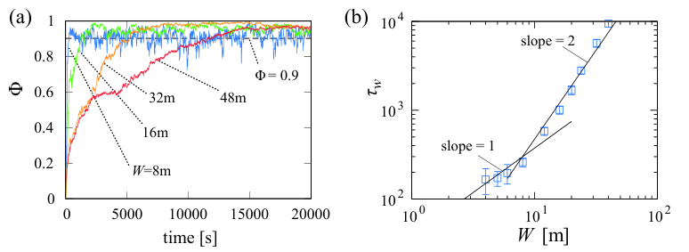
We next show in Fig. S9(a) the time evolution of obtained from simulations, starting from initial conditions in which pedestrians are randomly distributed (). The values of are plotted for various , fixing the obstacle angle and the average densities at and m-2, respectively. The systems show after reaching steady states, even for large values of (up to m, though not shown in the figure.) Then we examine the time taken to reach the steady states. In order to make a quantitative discussion, we define the relaxation time , the time interval taken from the initial state to reach . As we confirmed in Sec. S7, the long-time behavior of the pedestrians’ displacement in the -direction exhibits diffusion dynamics. Thus we expect for the range , i.e. for sufficiently wide corridors, and indeed this trend is observed in Fig. S9(b). On the other hand, our membrane model assumes that the density in each side of the corridor varies uniformely. In other words, we simplify the model by omitting the diffusion dynamics. The solution of the model is then obtained as follows:
| (8) |
where and are constants and is the stationary solution of the model. Here , because the steady solution corresponds the situation of , i.e., the pedestrians keep left and thus . Taking into account this with assuming as the value of the density corresponding , we find
| (9) |
This result implies . This analytical result is consistent with the behavior observed for relatively narrow corridor ( m) in Fig. S9(b).

In Fig. S10, we show the results for higher average density than that investigated in the main text: the mean velocity in (a) and the order parameter in (b). The parameter set is the same as Figs. 2 and 3 of the main text. The separation effect of is observed up to relatively high density m-2, although the effect tends to decay as increases. Accordingly the enhancement in velocity is obtained in this range of density. Next we show the effect of the screening parameter appearing in the social force model given in Eq. (2). Precisely the order parameter versus the angle is shown in Fig. S11 for different values of , in the case of m-2. The value of used thoroughly in the main text is m, which is the standard value used in the literature. Whereas the small value m shows the relatively weak impact on the results with slight enhancement of the separation effect, the value of higher than the standard one, m, weaken the separation effect giving smaller values of . This is because higher values of result in wider interaction ranges, and the size of the particles is thus larger. This variation of the particle size changes the effective average density. Indeed the model prediction matches the simulation results with adjusting the average density, m-2 for the case of m and m-2 for the case of m.