Mathematical Relativity
José Natário
Lisbon, 2020
Preface
These lecture notes were written for a one-semester course in mathematical relativity aimed at mathematics and physics students, which has been taught at Instituto Superior Técnico (Universidade de Lisboa) since 2010. They are not meant as an introduction to general relativity, but rather as a complementary, more advanced text, much like Part II of Wald’s textbook [Wal84], on which they are loosely based. It is assumed that the reader is familiar at least with special relativity, and has taken a course either in Riemannian geometry (typically the mathematics students) or in general relativity (typically the physics students). In other words, the reader is expected to be proficient in (some version of) differential geometry and to be acquainted with the basic principles of relativity.
I thank the many colleagues and students who read this text, or parts of it, for their valuable comments and suggestions. Special thanks are due to my colleague and friend Pedro Girão.
Chapter 1 Preliminaries
In this initial chapter we give a very short introduction to special and general relativity for mathematicians. In particular, we relate the index-free differential geometry notation used in Mathematics (e.g. [O’N83, dC93, Boo03, GN14]) to the index notation used in Physics (e.g. [MTW73, Wal84, HE95]). As an exercise in index gymnastics, we derive the contracted Bianchi identities.
1.1. Special relativity
Consider an inertial frame moving with velocity with respect to another inertial frame along their common -axis (Figure 1.1). According to classical mechanics, coordinate of a point on the frame is related to its coordinate on the frame by
Moreover, a clock in initially synchronized with a clock in is assumed to keep the same time:
Thus the spacetime coordinates of events are related by a so-called Galileo transformation

If the point is moving, its velocity in is related to its velocity in by
This is in conflict with the experimental fact that the speed of light is the same in every inertial frame, indicating that classical mechanics is not correct. Einstein solved this problem in 1905 by replacing the Galileo transformation by the so-called Lorentz transformation:
Here
and we are using units such that the speed of light is (for example measuring time in years and distance in light-years). Note that if is much smaller than the speed of light, , then , and we retrieve the Galileo transformation (assuming ).
Under the Lorentz transformation velocities transform as
In particular,
that is, the speed of light is the same in the two inertial frames.
In 1908, Minkowski noticed that
that is, the Lorentz transformations could be seen as isometries of with the indefinite metric
Definition 1.1.1.
The pseudo-Riemannian manifold is called the Minkowski spacetime.
Note that the set of vectors with zero square form a cone (the so-called light cone):
Definition 1.1.2.
A vector is said to be:
- (1)
timelike if ;
- (2)
spacelike if ;
- (3)
lightlike, or null, if .
- (4)
causal if it is timelike or null;
- (5)
future-pointing if it is causal and .
The same classification applies to (smooth) curves according to its tangent vector.

The length of a timelike (resp. spacelike) vector represents the time (resp. distance) measured between two events and in the inertial frame where these events happen in the same location (resp. are simultaneous). If is a timelike curve then its length
represents the proper time measured by the particle between events and . We have:
Proposition 1.1.3.
(Twin paradox) Of all timelike curves connecting two events , the curve with maximal length is the line segment (representing inertial motion).
Proof.
We may assume and on some inertial frame, and parameterize any timelike curve connecting to by the time coordinate:
Therefore
∎
Most problems in special relativity can be recast as questions about the geometry of the Minkowski spacetime.
Proposition 1.1.4.
(Doppler effect) An observer moving with velocity away from a source of light of period measures the period to be
Proof.
Figure 1.3 represents two light signals emitted by an observer at rest at with a time difference . These signals are detected by an observer moving with velocity , who measures a time difference between them. Now, if the first signal is emitted at , its history is the line . Consequently, the moving observer detects the signal at the event with coordinates

Similarly, the second light signal is emitted at , its history is the line , and it is detected by the moving observer at the event with coordinates
Therefore the time difference between the signals as measured by the moving observer is
∎
In particular, two observers at rest in an inertial frame measure the same frequency for a light signal (Figure 1.4). However, because the gravitational field couples to all forms of energy (as ), one expects that a photon climbing in a gravitational field to lose energy, hence frequency. In 1912, Einstein realized that this could be modelled by considering curved spacetime geometries, so that equal line segments in a (flat) spacetime diagram do not necessarily correspond to the same length.

1.2. Differential geometry: Mathematicians vs physicists
Einstein’s idea to incorporate gravitation into relativity was to replace the Minkowski spacetime by a curved four-dimensional Lorentzian manifold . Here is a Lorentzian metric, that is, a symmetric -tensor field such that at each tangent space in an appropriate basis. Just like in Riemannian geometry, determines a Levi-Civita connection, the unique connection which is symmetric and compatible with :
for all vector fields . The curvature of this connection is then given by the operator
The formulas above were written using the abstract notation usually employed by mathematicians. It is often very useful (especially when dealing with contractions) to use the more explicit notation usually adopted by physicists, which emphasizes the indices of the various objects when written in local coordinates:
| Object | Mathematicians | Physicists | ||
|---|---|---|---|---|
| Vector field | ||||
| Tensor product | ||||
| Metric | ||||
| Inner product | ||||
| Associated covector | ||||
| Covariant derivative | ||||
| Covariant derivative tensor |
Here are the Christoffel symbols of the Levi-Civita connection; they can be computed from the components of the metric tensor by the formula
and in turn be used to compute the components of the Riemann curvature tensor:
The covariant derivative tensor of a vector field , not always emphasized in differential geometry courses for mathematicians, is simply the -tensor field defined by
Also not always emphasized in differential geometry courses for mathematicians is the fact that any connection can be naturally extended to act on tensor fields (via the Leibnitz rule). For instance, if is a covector field (-form) then one defines
In local coordinates, this is
that is,
The generalization for higher rank tensors is obvious: for instance, if is a -tensor then
Note that the condition of compatibility of the Levi-Civita connection with the metric is simply
In particular, the operations of raising and lowering indices commute with covariant differentiation.
As an exercise in index gymnastics, we will now derive a series of identities involving the Riemann curvature tensor. We start by rewriting its definition in the notation of the physicists:
In other words,
or, equivalently,
| (1.1) |
where the square brackets indicate anti-symmetrization11 1 Thus , , etc.. This is readily generalized for arbitrary tensors: from
one readily concludes that
Let us choose
in equation (1.1). We obtain
because
Since we can choose arbitrarily at a given point, it follows that
This is the so-called first Bianchi identity, and is key for obtaining the full set of symmetries of the Riemann curvature tensor:
In the notation of the mathematicians, it is written as
for all vector fields .
Let us now take the covariant derivative of equation (1.1):
At any given point we can choose such that
Assuming this, we then obtain22 2 In the formula below the indices between vertical bars are not anti-symmetrized.
Since we can choose arbitrarily at a given point, it follows that
| (1.2) |
This is the so-called second Bianchi identity. In the notation of the mathematicians, it is written as
for all vector fields .
Recall that the Riemann curvature tensor has only one independent contraction, called the Ricci tensor:
The trace of the Ricci tensor, in turn, is known as the scalar curvature:
These quantities satisfy the so-called contracted Bianchi identity, which is obtained from (1.2) by contracting the pairs of indices and :
The contracted Bianchi identity is equivalent to the statement that the Einstein tensor
is divergenceless:
1.3. General relativity
Newtonian gravity is described by a scalar function , called the gravitational potential. The equation of motion for a free-falling particle of mass in Cartesian coordinates is
Note that all free-falling particles describe the same trajectories (an observation dating back to Galileo). The gravitational potential is determined from the matter mass density by the Poisson equation
(using units such that Newton’s gravitational constant is ; this choice, together with , defines the so-called geometrized units, where lengths, time intervals and masses all have the same dimensions).
To implement his idea of describing gravity via a curved four-dimensional Lorentzian manifold , Einstein had to specify how free-falling particles would move on this manifold, and how to determine the curved metric . Since free particles move along straight lines in the Minkowski spacetime, Einstein proposed that free falling particles should move along timelike geodesics. In other words, he suggested replacing the Newtonian equation of motion by the geodesic equation
Moreover, Einstein knew that it is possible to define the energy-momentum tensor of the matter content of the Minkowski spacetime, so that the conservation of energy and momentum is equivalent to the vanishing of its divergence:
This inspired Einstein to propose that should satisfy the so-called Einstein field equations:
Here is a constant, known as the cosmological constant. Note that the Einstein field equations imply, via the contracted Bianchi identity, that the energy-momentum tensor is divergenceless.
As a simple example, we consider a pressureless perfect fluid, known as dust. Its energy-momentum tensor is
where is the dust rest density and is a unit timelike vector field tangent to the histories of the dust particles. The equations of motion for the dust can be found from
Since and are orthogonal (because ), we find
in the support of . These are, respectively, the equation of conservation of mass and the geodesic equation. Thus the fact that free-falling particles move along geodesics can be seen as a consequence of the Einstein field equations (at least in this model).
1.4. Exercises
- (1)
Twin paradox: Two twins, Alice and Bob, are separated on their birthday. While Alice remains on Earth (which is an inertial frame to a very good approximation), Bob departs at of the speed of light towards Planet X, light-years away from Earth. Therefore Bob reaches his destination years later (as measured on the Earth’s frame). After a short stay, he returns to Earth, again at of the speed of light. Consequently Alice is years old when she sees Bob again.
- (a)
How old is Bob when they meet again?
- (b)
How can the asymmetry in the twins’ ages be explained? Notice that from Bob’s point of view he is at rest in his spaceship and it is the Earth which moves away and then back again.
- (c)
Imagine that each twin watches the other trough a very powerful telescope. What do they see? In particular, how much time do they experience as they see one year elapse for their twin?
- (a)
- (2)
A particularly simple matter model is that of a smooth massless scalar field , whose energy-momentum tensor is
Show that if the Lorentzian manifold satisfies the Einstein equations with this matter model then satisfies the wave equation
- (3)
The energy-momentum tensor for perfect fluid is
where is the fluid’s rest density, is the fluid’s rest pressure, and is a unit timelike vector field tangent to the histories of the fluid particles. Show that:
- (a)
in any orthonormal frame including ;
- (b)
the motion equations for the perfect fluid are
where ⟂ represents the orthogonal projection on the spacelike hyperplane orthogonal to .
- (a)
Chapter 2 Exact solutions
In this chapter we present a number of exact solutions of the Einstein field equations, as well as their Penrose diagrams. These solutions will be used as examples or counter-examples to the theorems in the subsequent chapters. We also discuss the matching of two different solutions across a timelike hypersurface. A different perspective on Penrose diagrams can be found in [HE95].
2.1. Minkowski spacetime
The simplest solution of the Einstein field equations with zero cosmological constant in vacuum (i.e. with vanishing energy-momentum tensor) is the Minkowski spacetime, that is, with the metric
Since this metric is flat, its curvature vanishes, and so do its Ricci and Einstein tensors. It represents a universe where there is no gravity whatsoever. Transforming the Cartesian coordinates to spherical coordinates yields
Performing the additional change of coordinates
we obtain
where
The coordinates are called null coordinates: their level sets are null cones formed by outgoing/ingoing null geodesics emanating from the center. Note that they are subject to the constraint
Finally, the coordinate change
| (2.1) |
brings the metric into the form
where now
and
| (2.2) |
Because are also null coordinates, it is common to represent their axes tilted by . The plane region defined by (2.2) is then represented in Figure 2.1.

This region is usually called the Penrose diagram for the Minkowski spacetime. If we take each point in the diagram to represent a sphere of radius , the diagram itself represents the full spacetime manifold, in a way that makes causality relations apparent: any causal curve is represented in the diagram by a curve with tangent at most from the vertical. In Figure 2.2 we represent some level hypersurfaces of and in the Penrose diagram. The former approach the point in the boundary of the diagram, called the spacelike infinity, whereas the later go from the boundary point (past timelike infinity) to the boundary point (future timelike infinity). Finally, null geodesics start at the null boundary line (past null infinity) and end at the null boundary line (future null infinity). These boundary points and lines represent ideal points at infinity, and do not correspond to actual points in the Minkowski spacetime.

2.2. Penrose diagrams
The concept of Penrose diagram can be easily generalized for any spherically symmetric space-time. Such spacetimes have metric
where is a Lorentzian metric on a -dimensional quotient manifold with boundary (which we assume to be diffeomorphic to a region of the plane). It turns out that any such metric is conformal to the Minkowski metric:
| (2.3) |
This can be seen locally as follows: choose a spacelike line , a coordinate along it, and a coordinate along a family of null geodesics emanating from , so that corresponds to (Figure 2.3). Then near we have
and

Therefore the -dimensional metric is written in these coordinates
As for any -form in a -dimensional manifold, we have
for suitable functions and . Note that cannot vanish, because are local coordinates. Moreover, we can assume by replacing with if necessary. Choosing then yields (2.3).
We then see that any spherically symmetric metric can be written as
| (2.4) |
with and . By rescaling and if necessary, we can assume that the range of is bounded, and hence obtain a Penrose diagram depicting the causal geometry. As we will see, this is extremely helpful in more complicated spherical symmetric solutions of the Einstein field equations.
Remark 2.2.1.
From
it is easily seen that
and similarly for . In other words, the null coordinates and are solutions of the wave equation in the -dimensional Lorentzian manifold:
This is the Lorentzian analogue of the so-called isothermal coordinates for Riemannian surfaces. The proof that the later exist locally is however slightly more complicated: given a point on the surface, one chooses a local harmonic function with nonvanishing derivative,
and considers the equation
| (2.5) |
Here is the Hodge star, which for generic orientable -dimensional pseudo-Riemannian manifolds is defined as follows: if is any positively oriented orthonormal coframe then
By the Poincaré Lemma, equation (2.5) can be locally solved, since
Moreover, is itself harmonic, because
Finally,
for some local function , and so the metric is written is these coordinates as
2.3. The Schwarzschild solution
If we try to solve the vacuum Einstein field equations with zero cosmological constant for a spherically symmetric Lorentzian metric, we obtain, after suitably rescaling the time coordinate, the Schwarzschild metric
(where is a constant). Note that for we retrieve the Minkowski metric in spherical coordinates. Note also that if then the metric is defined in two disconnected domains of coordinates, corresponding to and .
The physical interpretation of the Schwarzschild solution can be found by considering the proper time of a timelike curve parameterized by the time coordinate:
where , etc. The integrand is the Lagrangian for geodesic motion in the Schwarzschild spacetime when parameterized by the time coordinate. Now for motions with speeds much smaller than the speed of light we have , etc. Assuming as well we have
where
is precisely the Newtonian Lagrangian for the motion of a particle in the gravitational field of a point mass . The Schwarzschild solution should therefore be considered the relativistic analogue of this field.
To write the Schwarzschild metric in the form (2.4) we note that the quotient metric is
where we define
and
In the domain of coordinates we have , and so the quotient metric is already in the required form. Note however that, unlike what happened in the Minkowski spacetime, we now have
Consequently, by applying the coordinate rescaling (2.1) we obtain the full square, instead of a triangle (Figure 2.4). Besides the infinity points and null boundaries also present in the Penrose diagram for the Minkowski spacetime, there are two new null boundaries, (past event horizon) and (future event horizon), where .

It seems reasonable to expect that the metric can be extended across the horizons, since does not tend to zero nor to infinity there; this expectation is confirmed by calculating the so-called Kretschmann scalar:
This is perfectly well behaved as , and seems to indicate that the horizons are mere singularities of the coordinate system . To show that this is indeed the case, note that in the coordinate system the quotient metric is written
Since
we see that the metric is well defined across in this coordinate system. Moreover, we know that it solves the Einstein equations in the coordinate domains and ; by continuity, it must solve it in the whole domain . Note that the coordinate domains and are glued along so that the outgoing null geodesics go from to ; in other words, the gluing is along the past event horizon .
To obtain the Penrose diagram for the coordinate domain we note that the quotient metric can be written as
where . Since in this coordinate domain , the quotient metric is in the required form. Note however that we now have
and by setting
we obtain
Consequently, by applying the coordinate rescaling (2.1) we obtain a triangle (Figure 2.5). There is now a spacelike boundary, where , and two null boundaries , where . The Penrose diagram for the domain of the coordinates can be obtained gluing the Penrose diagrams in Figures 2.4 and 2.5 along , so that the null geodesics match (Figure 2.6).


If instead we use the coordinate system, the quotient metric is written
Again the metric is well defined across in this coordinate system, since
and solves the Einstein equations in the whole coordinate domain . The coordinate domains and are now glued along so that the ingoing null geodesics go from to ; in other words, the gluing is along the future event horizon .
To obtain the Penrose diagram for the coordinate domain we note that the quotient metric can be written as
where . Since in this coordinate domain , the quotient metric is in the required form. We have
and by setting
we obtain
Consequently, by applying the coordinate rescaling (2.1) we obtain a triangle (Figure 2.7). Again there is a spacelike boundary, where , and two null boundaries , where . The Penrose diagram for the domain of the coordinates can be obtained gluing the Penrose diagrams in Figures 2.4 and 2.7 along , so that the null geodesics match (Figure 2.8).


Both regions can of course be glued to the region simultaneously. Since they are invariant under reflections with respect to (the vertical line through their common vertex), it is then clear that a mirror-reversed copy of the region can be glued to the surviving null boundaries and (Figure 2.9). The resulting spacetime, known as the maximal analytical extension of the Schwarzschild solution, is a solution of the Einstein equations which cannot be extended any further, since or on the boundary of its Penrose diagram. Note that by continuity the Einstein equations hold at the point where the four Penrose diagrams intersect (known as the bifurcate sphere).

Let us now analyze in detail the Penrose diagram for the maximal analytic extension of the Schwarzschild spacetime. There are two asymptotically flat regions , corresponding to two causally disconnected universes, joined by a wormhole. There are also two regions where : a black hole region, bounded by the future event horizons , from which no causal curve can escape; and a white hole region, bounded by the past event horizons , from which every causal curve must escape. Note that the horizons themselves correspond to spheres which are propagating at the speed of light, but whose radius remains constant, .
The black hole in the maximal analytic extension of the Schwarzschild spacetime is an eternal black hole, that is, a black hole which has always existed (as opposed to having formed by some physical process). We will see shortly how to use the Schwarzschild solution to model physically realistic black holes.
2.4. Friedmann-Lemaître-Robertson-Walker models
The simplest models of cosmology, the study of the Universe as a whole, are obtained from the assumption that space is homogeneous and isotropic (which is true on average at very large scales). It is well known that the only isotropic -dimensional Riemannian metrics are, up to scale, given by
where
Allowing for a time-dependent scale factor (also known as the “radius of the Universe”), we arrive at the Friedmann-Lemaître-Robertson-Walker (FLRW) family of Lorentzian metrics:
| (2.6) |
To interpret these metrics, we consider a general Lorentzian metric of the form
The Riemannian metric is readily interpreted as giving the distances measured between nearby observers with fixed space coordinates in radar experiments: indeed, such observers measure proper time given by
The null geodesics representing a radar signal bounced by a given observer from a nearby observer (Figure 2.10) satisfy

Since the speed of light is , the distance traveled between the observers will be half the time between the emission and the reception of the signal:
Moreover, the unit timelike covector field tangent to the trajectories of the the observers with fixed space coordinates is
Therefore
since . In other words,
where ⟂ represents the orthogonal projection on the spacelike hyperplane orthogonal to .
Therefore the observers with fixed space coordinates in the FLRW models have zero acceleration, that is, they are free-falling (by opposition to the corresponding observers in the Schwarzschild spacetime, who must accelerate to remain at fixed ). Moreover, the distance between two such observers varies as
This relation, known as the Hubble law, is often written as
where is the relative velocity and
is the so-called Hubble constant (for historical reasons, since it actually varies in time).
We will model the matter content of the universe as an uniform dust of galaxies placed at fixed space coordinates (hence free-falling):
| (2.7) |
Plugging the metric (2.6) and the energy-momentum tensor (2.7) into the Einstein equations, and integrating once, results in the so-called Friedmann equations
(where is an integration constant). The first Friedmann equation is a first order ODE for ; it can be seen as the equation of conservation of energy for a particle moving in the -dimensional effective potential
with energy . Once this equation has been solved, the second Friedmann equation yields from . We now examine in detail the FLRW models arising from the solutions of these equations.
2.4.1. Milne universe
If we set then the first Friedmann equation becomes
Therefore either and , which corresponds to the Minkowski spacetime, or and , that is
where represents the metric of the unit hyperbolic -space; this is the so-called Milne universe. It turns out that the Milne universe is isometric to an open region of the Minkowski spacetime, namely the region limited by the future (or past) light cone of the origin. This region is foliated by hyperboloids of the form
whose induced metric is that of a hyperbolic space of radius (Figure 2.11). Note that the light cone corresponds to , that is, the Big Bang of the Milne universe.

2.4.2. de Sitter universe
If and we can choose units such that . The first Friedmann equation then becomes
In this case all three values , and are possible; the corresponding metrics are, respectively,
where , and represent the metric of the unit -sphere, the Euclidean -space and the the unit hyperbolic -space.
It turns out that the last two models correspond to open regions of the first, which is then called the de Sitter universe. It represents a spherical universe which contracts to a minimum radius ( in our units) and then re-expands. It is easily seen to be isometric to the unit hyperboloid
in the Minkowski -dimensional spacetime (Figure 2.12).

To obtain the Penrose diagram for the de Sitter universe we write its metric as
where ,
and
Since
we see that the quotient metric is conformal to the square of the Minkowski -dimensional spacetime, and so the Penrose diagram is as depicted in Figure 2.12. Note that there are two lines where , corresponding to two antipodal points of the -sphere. A light ray emitted from one of these points at has just enough time to reach the other point at (dashed line in the diagram). Note also that in this case and (defined as the past and future boundary points approached by null geodesics along which ) are spacelike boundaries.

2.4.3. Anti-de Sitter universe
If and we can choose units such that . The the first Friedmann equation then becomes
In this case only is possible; the corresponding metric is
It turns out (see Exercise 5 in Chapter 5) that this model is an open region of the spacetime with metric
(where ), called the anti-de Sitter universe. It represents a static hyperbolic universe (with radius in our units).
To obtain the Penrose diagram for the anti-de Sitter universe we write its metric as
where
and
Since
we see that the quotient metric is conformal to the strip of the Minkowski -dimensional spacetime, and so the Penrose diagram is as depicted in Figure 2.14. The FLRW model above corresponds to the triangular region in the diagram. Note also that in this case is a timelike boundary.

2.4.4. Universes with matter and
If and , the first Friedmann equation becomes
In this case all three values , and are possible. Although it is possible to obtain explicit formulas for the solutions of these equations, it is simpler to analyze the graph of the effective potential (Figure 2.15). Possibly by reversing and translating , we can assume that all solutions are defined for , with , implying . Therefore all three models have a true singularity at , known as the Big Bang, where the scalar curvature also blows up; this is not true for the Milne universe or the open region in the anti-de Sitter universe, which can be extended across the Big Bang. The spherical universe () reaches a maximum radius and re-collapses, forming a second singularity (the Big Crunch); the radius of the flat () and hyperbolic () universes increases monotonically.

To obtain the Penrose diagram for the spherical universe we write its metric as
where ,
and
Since
we see that the quotient metric is conformal to the rectangle of the Minkowski -dimensional spacetime, and so the Penrose diagram is as depicted in Figure 2.16. Note that there are two lines where , corresponding to two antipodal points of the -sphere. A light ray emitted from one of these points at has just enough time to circle once around the universe an return at (dashed line in the diagram). Note also that the Big Bang and the Big Crunch are spacelike boundaries.

To obtain the Penrose diagram for the flat universe we write its metric as
where and . Since
we see that the quotient metric is conformal to the region of the Minkowski -dimensional spacetime, and so the Penrose diagram is as depicted in Figure 2.17. Note that the Big Bang is a spacelike boundary.

The Penrose diagram for the hyperbolic universe turns out to be the same as for the flat universe. To see this we write its metric as
where and , and note that
2.4.5. Universes with matter and
If and we can choose units such that . The first Friedmann equation then becomes
In this case all three values , and are possible. As before, we analyze the graph of the effective potential (Figure 2.18). The hyperbolic and flat universes behave qualitatively like when , although is now unbounded as , instead of approaching some constant. The spherical universe has a richer spectrum of possible behaviors, depending on , represented in Figure 2.18 by drawing the line of constant energy at three different heights. The higher line (corresponding to ) yields a behaviour similar to that of the hyperbolic and flat universes. The intermediate line (corresponding to ) gives rise to an unstable equilibrium point , where the attraction force of the matter is balanced by the repulsion force of the cosmological constant; it corresponds to the so-called Einstein universe, the first cosmological model ever proposed. The intermediate line also yields two solutions asymptotic to the Einstein universe, one containing a Big Bang and the other endless expansion. Finally, the lower line (corresponding to ) yields two different types of behaviour (depending on the initial conditions): either similar to the spherical model with , or to the de Sitter universe.

It is currently believed that the best model for our physical Universe is the the flat universe with . If we write the first Friedmann equation as
then the terms on the right-hand side are in the proportion at the present time.
2.4.6. Universes with matter and
If and we can choose units such that . The first Friedmann equation then becomes
In this case all three values , and are possible. As before, we analyze the graph of the effective potential (Figure 2.19). The qualitative behaviour of the hyperbolic, flat and spherical universes is the same as the spherical universe with , namely starting at a Big Bang and ending at a Big Crunch.

2.5. Matching
Let and be solutions of the Einstein field equations containing open sets and whose boundaries and are timelike hypersurfaces, that is, hypersurfaces whose induced metric is Lorentzian (or, equivalently, whose normal vector is spacelike). If is diffeomorphic to then we can identify them to obtain a new manifold gluing to along (Figure 2.20).

Let be the unit normal vector to pointing out of , which we identify with the unit normal vector to pointing into . If are local coordinates on , we can construct a system of local coordinates in a neighbourhood of by moving a distance along the geodesics with initial condition . Note that , and correspond to , and in these coordinates. Since is the unit tangent vector to the geodesics, we have
(), where we used
Since for we have
we see that remains orthogonal to the surfaces of constant . This result will be used repeatedly.
Lemma 2.5.1.
(Gauss Lemma I) Let be a Riemannian or a Lorentzian manifold, and a hypersurface whose normal vector field satisfies . The hypersurfaces obtained from by moving a distance along the geodesics orthogonal to remain orthogonal to the geodesics.
The same ideas can be used to prove a closely related result.
Lemma 2.5.2.
(Gauss Lemma II) Let be a Riemannian or a Lorentzian manifold and . The hypersurfaces obtained from by moving a distance along the geodesics through remain orthogonal to the geodesics.
In this coordinate system the metrics and are given on and , respectively, by
(). Therefore we can define a continuous metric on if
that is, if
This also guarantees continuity of all tangential derivatives of the metric, but not of the normal derivatives. In order to have a metric we must have
that is,
Note that in this case the curvature tensor (hence the energy-momentum tensor) is at most discontinuous across . More importantly, as shown in Exercise 8, the components and of the energy-momentum tensor are continuous across (that is, the flow of energy and momentum across is equal on both sides), implying that the energy-momentum tensor satisfies the integral version of the conservation equation . Therefore we can consider a solution of the Einstein equations.
Recall that
is known as the extrinsic curvature, or second fundamental form, of . We can summarize the discussion above in the following statement.
Proposition 2.5.3.
Two solutions and of the Einstein field equations can be matched along diffeomorphic timelike boundaries and if and only if the induced metrics and second fundamental forms coincide:
2.6. Oppenheimer-Snyder collapse
We can use the matching technique to construct a solution of the Einstein field equations which describes a spherical cloud of dust collapsing to a black hole. This is a physically plausible model for a black hole, as opposed to the eternal black hole.
Let us take to be a flat collapsing FLRW universe:
We choose to be the hypersurface , with normal vector
The induced metric then is
and the second fundamental form
Here we used Cartan’s magic formula: if is a differential form and is a vector field then
Thus, for example,
Note that the function is constrained by the first Friedmann equation:
| (2.8) |
(we assume ).
We now take to be the Schwarzschild solution,
where
and choose to be a spherically symmetric timelike hypersurface given by the parameterization
The exact form of the functions and will be fixed by the matching conditions; for the time being they are constrained only by the condition that is the proper time along :
The induced metric is then
and so the two induced metrics coincide if and only if
| (2.9) |
To simplify the calculation of the second fundamental form, we note that since is ruled by timelike geodesics, so is , because the induced metrics and extrinsic curvatures are the same (therefore so are the Christoffel symbols). Therefore and must be a solution of the radial geodesic equations, which are equivalent to
| (2.10) |
(where is a constant). Equations (2.8), (2.9) and (2.10) are compatible if and only if
that is, if and only if represents a spherical shell dropped from infinity with zero velocity and the mass parameter of the Schwarzschild spacetime is related to the density of the collapsing dust by
To compute the second fundamental form of we can then consider a family of free-falling spherical shells which includes . If is the parameter indexing the shells (with corresponding to, say, ) then by the Gauss Lemma we can write the Schwarzschild metric in the form
(consider, for instance, the change of coordinates determined by the solution , of the radial geodesic equations with initial conditions determined by , , ). The unit normal vector field to the hypersurfaces of constant is then
and so we have
On the other hand, in Schwarzschild coordinates
since must be unit and orthogonal to
Therefore we have
or, using ,
In other words, follows from the previous conditions, and so we indeed have a solution of the Einstein equations.

To construct the Penrose diagram for this solution we represent and in the Penrose diagrams of the collapsing flat FLRW universe (obtained by reversing the time direction in the expanding flat FLRW universe) and the Schwarzschild solution (Figure 2.21). Identifying these hypersurfaces results in the Penrose diagram depicted in Figure 2.22.

2.7. Exercises
- (1)
In this exercise we will solve the vacuum Einstein equations (without cosmological constant) for the spherically symmetric Lorentzian metric given by
where and are positive smooth functions.
- (a)
Use Cartan’s first structure equations,
to show that the nonvanishing connection forms for the orthonormal frame dual to
are (using the notation and )
- (b)
Use Cartan’s second structure equations,
to show that the curvature forms on this frame are
- (c)
Using
determine the components of the curvature tensor in this orthonormal frame, and show that the nonvanishing components of the Ricci tensor in this frame are
Conclude that the nonvanishing components of the Einstein tensor in this frame are
- (d)
Show that if we write
for some smooth function then
Conclude that the Einstein equations are equivalent to
where is an integration constant.
- (e)
Show that the Einstein equation is equivalent to for some positive smooth function .
- (f)
Check that if and are as above then the remaining Einstein equations are automatically satisfied.
- (g)
Argue that it is always possible to rescale the time coordinate so that the metric is written
(the statement that any spherically symmetric solution of the vacuum Einstein equations without cosmological constant is of this form is known as Birkhoff’s theorem).
- (a)
- (2)
Show that the Riemannian manifold obtained by gluing the hypersurfaces of the two exterior regions in the maximally extended Schwarzschild solution along the horizon is isometric to the Flamm paraboloid, that is, the hypersurface in with equation
(Figure 2.23).

Figure 2.23. Two-dimensional analogue of the Flamm paraboloid. - (3)
Recall that the nonvanishing components of the Einstein tensor of the spherically symmetric Lorentzian metric
in the orthonormal frame dual to
are given by (using the notation and )
where
- (a)
Assuming
- •
(so that , and hence , do not depend on );
- •
(so that for some positive smooth function );
- •
(which can always be achieved by rescaling ),
show that
- •
- (b)
Prove that the general spherically symmetric solution of the vacuum Einstein field equations with a cosmological constant is the Kottler metric
- (c)
Obtain the Penrose diagram for the maximal extension of the Kottler solution with and .
- (d)
Consider now the spherically symmetric electromagnetic field
Show that this field satisfies the vacuum Maxwell equations
(where is the Hodge star) if and only if
for some constant (the electric charge in units for which ).
- (e)
As we shall see in Chapter 6, this electromagnetic field corresponds to the energy-momentum tensor
Prove that the general spherically symmetric solution of the Einstein field equations with an electromagnetic field of this kind is the Reissner-Nordström metric
- (f)
Obtain the Penrose diagram for the maximal extension of the Reissner-Nordström solution with and .
- (a)
- (4)
Consider the spherically symmetric Lorentzian metric
where is a positive smooth function.
- (a)
Use Cartan’s first structure equations,
to show that the nonvanishing connection forms for the orthonormal frame dual to
are
- (b)
Use Cartan’s second structure equations,
to show that the curvature forms on this frame are
- (c)
Using
determine the components of the curvature tensor on this orthonormal frame, and show that the nonvanishing components of the Ricci tensor on this frame are
Conclude that the nonvanishing components of the Einstein tensor on this frame are
- (d)
Show that the Einstein equations with a cosmological constant for a comoving pressureless perfect fluid of nonnegative density , , are equivalent to the system
Show that this system can be integrated to
where is a nonnegative integration constant.
- (e)
Draw the Penrose diagram of the solutions with , and (currently believed to model our physical Universe).
- (a)
- (5)
Compute the metrics of the following manifolds in the local coordinates indicated, and sketch the corresponding Penrose diagrams:
- (a)
The region of the -dimensional Minkowski spacetime using the parameterization
- (b)
The hyperboloid in the -dimensional Minkowski spacetime using the parameterization
- (c)
The region of the same hyperboloid using the parameterization
- (d)
The region of the same hyperboloid using the parameterization defined implicitly by
- (e)
The hyperboloid in with the pseudo-Riemannian metric
using the parameterization
- (a)
- (6)
Show that the anti-de Sitter metric
is a solution of the vacuum Einstein field equations with cosmological constant .
- (7)
The -dimensional anti-de Sitter space can be obtained by “unwrapping” the hyperboloid in with the pseudo-Riemannian metric
In this exercise we identify with the space of matrices by the map
- (a)
Show that the hyperboloid corresponds to the Lie group of matrices with unit determinant.
- (b)
Check that the squared norm of a vector in the metric above is , where is the matrix associated to . Conclude that the metric induced on the hyperboloid is bi-invariant (that is, invariant under left and right multiplication).
- (c)
Use the Penrose diagram in Figure 2.24 and the fact that the one-parameter subgroups of a Lie group with a bi-invariant metric are geodesics of that metric to conclude that the exponential map is not surjective.
- (d)
Write explicitly the matrices in which are not in the image of by using the parameterization

Figure 2.24. Exponential map on . - (a)
- (8)
Consider a Riemannian or Lorentzian metric given in the Gauss Lemma form
so that the level sets of are Riemannian or Lorentzian manifolds with induced metric and second fundamental form
Show that in these coordinates:
- (a)
The Christoffel symbols are
where are the Christoffel symbols of .
- (b)
The components of the Riemann tensor are
where is the Levi-Civita connection of and are the components of the Riemann tensor of .
- (c)
The time derivative of the inverse metric is given by the formula
- (d)
The components of the Ricci tensor are
where are the components of the Ricci tensor of .
- (e)
The scalar curvature is
where is the scalar curvature of .
- (f)
The component of the Einstein tensor is
This shows that the matching conditions guarantee the continuity of and .
- (a)
- (9)
Recall that the nonvanishing components of the Einstein tensor of the static, spherically symmetric Lorentzian metric
in the orthonormal frame dual to
are given by
where
In this exercise we will solve the Einstein equations (without cosmological constant) for a static perfect fluid of constant rest density and rest pressure , and match it to a Schwarzschild exterior.
- (a)
Show that
where . Conclude that the spatial metric is that of a sphere with radius .
- (b)
Solve the ordinary differential equation to obtain
where are integration constants.
- (c)
Show that the matching conditions to a Schwarzschild exterior of mass across a surface are
- (d)
Conclude that
- (e)
Show that
What is the value of ?
- (f)
Show that and must satisfy Buchdahl’s limit:
What happens to as ?
- (a)
Chapter 3 Causality
In this chapter we briefly discuss the causality theory of a Lorentzian manifold, following [GN14]. We take a minimal approach; more details can be found in [O’N83, Wal84, Pen87, Nab88, HE95, Rin09].
3.1. Past and future
A spacetime is said to be time-orientable if there exists a timelike vector field, that is, a vector field satisfying . In this case, we can define a time orientation on each tangent space by declaring causal vectors to be future-pointing if . It can be shown that any non-time-orientable spacetime admits a time-orientable double covering (just like any non-orientable manifold admits an orientable double covering).
Assume that is time-oriented (i.e. time-orientable with a definite choice of time orientation). A timelike or causal curve is said to be future-directed if is future-pointing. The chronological future of is the set of all points to which can be connected by a future-directed timelike curve. The causal future of is the set of all points to which can be connected by a future-directed causal curve. Notice that is simply the set of all events which are accessible to a particle with nonzero mass at , whereas is the set of events which can be causally influenced by (as this causal influence cannot propagate faster than the speed of light). Analogously, the chronological past of is the set of all points which can be connected to by a future-directed timelike curve, and the causal past of is the set of all points which can be connected to by a future-directed causal curve.
In general, the chronological and causal pasts and futures can be quite complicated sets, because of global features of the spacetime. Locally, however, causal properties are similar to those of Minkowski spacetime. More precisely, we have the following statement:
Proposition 3.1.1.
Let be a time-oriented spacetime. Then each point has an open neighborhood such that the spacetime obtained by restricting to satisfies:
- (1)
is geodesically convex, that is, is a normal neighborhood of each of its points such that given there exists a unique geodesic (up to reparameterization) connecting to ;
- (2)
if and only if there exists a future-directed timelike geodesic connecting to ;
- (3)
;
- (4)
if and only if there exists a future-directed null geodesic connecting to .
Proof.
Recall that the exponential map is the map given by
where is the geodesic with initial conditions , ; equivalently, (since ). Recall also that is a normal neighborhood of if is a diffeomorphism. The existence of geodesically convex neighborhoods is true for any affine connection and is proved for instance in [KN96].
To prove assertion (2), we start by noticing that if there exists a future-directed timelike geodesic connecting to then it is obvious that . Suppose now that ; then there exists a future-directed timelike curve such that and . Choose normal coordinates , given by the parameterization
where is an orthonormal basis of with timelike and future-pointing. These are global coordinates in , since is a diffeomorphism. Defining
with , we have to show that . Let . Since , we have . Setting , we obtain
and consequently
Therefore there exists such that for .
By the Gauss Lemma, the level surfaces of are orthogonal to the geodesics through . Therefore, if is the geodesic with initial condition , we have
Now
and hence
On the other hand,
We conclude that , and therefore
Consequently, is tangent to geodesics through , being future-pointing on future-directed geodesics.
Suppose that . Then is timelike future-pointing, and so
as is also timelike future-pointing. We conclude that we must have for all . In particular, , and hence there exists a future-directed timelike geodesic connecting to .
To prove assertion (3), let us see first that . If , then is the limit of a sequence of points . By (2), with timelike future-pointing. Since is a diffeomorphism, converges to a causal future-pointing vector , and so can be reached from by a future-directed causal geodesic. The converse inclusion holds in general (cf. Proposition 3.1.2).
Finally, (4) is obvious from (3) and the fact that is a diffeomorphism onto . ∎
This local behavior can be used to prove the following global result.
Proposition 3.1.2.
Let be a time oriented spacetime and . Then:
- (1)
is open;
- (2)
;
- (3)
- (4)
if and then ;
- (5)
if and then .
Proof.
Exercise. ∎
The twin paradox also holds locally for general spacetimes. More precisely, we have the following statement:
Proposition 3.1.3.
Let be a time-oriented spacetime, and a geodesically convex open neighborhood of . The spacetime obtained by restricting to satisfies the following property: if with , is the timelike geodesic connecting to and is any timelike curve connecting to , then , with equality if and only if is a reparameterization of .
Proof.
Any timelike curve satisfying , can be written as
for , where and . We have
Since , we have , and consequently is tangent to the level surfaces of the function . We conclude that
where is the unit tangent vector field to timelike geodesics through and is tangent to the level surfaces of (hence orthogonal to ). Consequently,
where we have used the facts that is timelike, for all (as is future-pointing) and (as ). It should be clear that if and only if ( is spacelike or zero) for all , implying that is constant. In this case, is, up to reparameterization, the geodesic through with initial condition . ∎
There is also a local property characterizing null geodesics.
Proposition 3.1.4.
Let be a time-oriented spacetime, and a geodesically convex open neighborhood of . The spacetime obtained by restricting to satisfies the following property: if for there exists a future-directed null geodesic connecting to and is a causal curve connecting to then is a reparameterization of .
Proof.
Since and are connected by a null geodesic, we conclude from Proposition 3.1.1 that . Let be a causal curve connecting to . Then we must have for all , since implies for all (see Proposition 3.1.2). Consequently, we have
where was defined in the proof of Proposition 3.1.1. The formula
which was proved for timelike geodesics with initial condition , must also hold for null geodesics (by continuity). Hence is tangent to the null geodesics ruling and future-pointing. Since is also future-pointing, we conclude that is proportional to , and therefore is a reparameterization of a null geodesic, which must be . ∎
Corollary 3.1.5.
Let be a time-oriented spacetime and . If then any future-directed causal curve connecting to must be a reparameterized null geodesic.
3.2. Causality conditions
For physical applications, it is important to require that the spacetime satisfies reasonable causality conditions. The simplest of these conditions excludes time travel, i.e. the possibility of a particle returning to an event in its past history.
Definition 3.2.1.
A spacetime is said to satisfy the chronology condition if it does not contain closed timelike curves.
This condition is violated by compact spacetimes:
Proposition 3.2.2.
Any compact spacetime contains closed timelike curves.
Proof.
Taking if necessary the time-orientable double covering, we can assume that is time-oriented. Since is an open set for any , it is clear that is an open cover of . If is compact, we can obtain a finite subcover . Now if for then , and we can exclude from the subcover. Therefore, we can assume without loss of generality that , and hence there exists a closed timelike curve starting and ending at . ∎
A stronger restriction on the causal behavior of the spacetime is the following:
Definition 3.2.3.
A spacetime is said to be stably causal if there exists a global time function, i.e. a smooth function such that is timelike.
In particular, a stably causal spacetime is time-orientable. We choose the time orientation defined by , so that increases along future-directed timelike curves. Notice that this implies that no closed timelike curves can exist, i.e. any stably causal spacetime satisfies the chronology condition. In fact, any small perturbation of a stably causal spacetime still satisfies the chronology condition (Exercise 4).
Let be a time-oriented spacetime. A smooth future-directed causal curve (with possibly or ) is said to be future-inextendible if does not exist. The definition of a past-inextendible causal curve is analogous. The future domain of dependence of is the set of all events such that any past-inextendible causal curve starting at intersects . Therefore any causal influence on an event had to register somewhere in , and one can expect that what happens at can be predicted from data on . Similarly, the past domain of dependence of is the set of all events such that any future-inextendible causal curve starting at intersects . Therefore any causal influence of an event will register somewhere in , and one can expect that what happened at can be retrodicted from data on . The domain of dependence of is simply the set .
Let be a stably causal spacetime with time function . The level sets are said to be Cauchy hypersurfaces if . Spacetimes for which this happens have particularly good causal properties.
Definition 3.2.4.
A stably causal spacetime possessing a time function whose level sets are Cauchy hypersurfaces is said to be globally hyperbolic.
Notice that the future and past domains of dependence of the Cauchy hypersurfaces are and .
3.3. Exercises
- (1)
Let be the quotient of the -dimensional Minkowski spacetime by the discrete group of isometries generated by the map . Show that is not time orientable.
- (2)
Let be a time oriented spacetime and . Show that:
- (a)
is open;
- (b)
is not necessarily closed;
- (c)
;
- (d)
- (e)
if and then ;
- (f)
if and then .
- (a)
- (3)
Consider the -dimensional Minkowski spacetime , where
Let be the curve . Show that although is null for all we have for all . What kind of motion does this curve represent?
- (4)
Let be a stably causal spacetime and an arbitrary symmetric -tensor field with compact support. Show that for sufficiently small the tensor field is still a Lorentzian metric on , and satisfies the chronology condition.
- (5)
Let be the quotient of the -dimensional Minkowski spacetime by the discrete group of isometries generated by the map . Show that satisfies the chronology condition, but there exist arbitrarily small perturbations of (in the sense of Exercise 4) which do not.
- (6)
Let be a time oriented spacetime and . Show that:
- (a)
;
- (b)
is not necessarily open;
- (c)
is not necessarily closed.
- (a)
- (7)
Let be the -dimensional spacetime obtained by removing the positive -semi-axis of Minkowski -dimensional spacetime (cf. Figure 3.1). Show that:
- (a)
is stably causal but not globally hyperbolic;
- (b)
there exist points such that is not compact;
- (c)
there exist points with such that the supremum of the lengths of timelike curves connecting to is not attained by any timelike curve.

Figure 3.1. Stably causal but not globally hyperbolic spacetime. - (a)
- (8)
Let be a -dimensional Riemannian manifold. Show that the spacetime is globally hyperbolic if and only if is complete.
- (9)
Show that the following spacetimes are globally hyperbolic:
- (a)
the Minkowski spacetime;
- (b)
the FLRW spacetimes;
- (c)
the region of the Schwarzschild spacetime;
- (d)
the region of the Schwarzschild spacetime;
- (e)
the maximal analytical extension of the Schwarzschild spacetime.
- (a)
- (10)
Let be a global hyperbolic spacetime with Cauchy hypersurface . Show that is diffeomorphic to .
Chapter 4 Singularity theorems
As we have seen in Chapter 2, both the Schwarzschild solution and the FLRW cosmological models display singularities, beyond which timelike and null geodesics cannot be continued. It was once thought that these solutions were singular due to their high degree of symmetry, and that more realistic spacetimes would be non-singular. In this chapter we show that this is not the case: any sufficiently small perturbation of these solutions will still be singular. We follow [Wal84] when discussing conjugate points and [GN14] for the details of the proofs. See also [O’N83, Pen87, Nab88, HE95].
4.1. Geodesic congruences
Let be a Lorentzian manifold. A congruence of curves in an open set is the family of integral curves of a nonvanishing vector field in . We will assume that is unit timelike and geodesic, that is,
The properties of the congruence determined by are best analyzed by considering its second fundamental form
This tensor is purely spatial, that is,
Indeed, since is unit,
On the other hand, because is geodesic,
Proposition 4.1.1.
The second fundamental form satisfies
Proof.
We have
∎
Let be a one-parameter family of geodesics of the congruence, parameterized such that
(Figure 4.1). The geodesic deviation vector associated to is
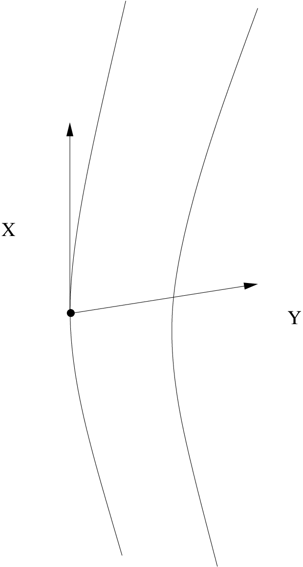
Proposition 4.1.2.
The geodesic deviation vector satisfies
Proof.
The definition of implies that
Consequently, we have
∎
The equation for then yields the following famous result.
Proposition 4.1.3.
The geodesic deviation vector satisfies the Jacobi equation
Proof.
We have
Alternatively, we can simply notice that
∎
We now define the kinematic quantities associated to the congruence.
Definition 4.1.4.
The spatial metric associated to the congruence is
The expansion, shear and vorticity are defined as11 1 Curved brackets indicate symmetrization: .
so that we have the decomposition
Note that all the tensors above are purely spatial:
Moreover, the trace of is
and so the shear is traceless:
Fix a geodesic , and let be a geodesic deviation vector along . If is initially orthogonal to then it will remain orthogonal:
In an orthonormal frame parallel along we then have
(). If we consider a small spacelike sphere in the hypersurface orthogonal to and let it be carried by the geodesics of the congruence, we see that measures the rate at which the sphere’s volume grows, describes the sphere’s volume-preserving shape deformations, and gives the sphere’s angular velocity.
Proposition 4.1.5.
The expansion of the congruence satisfies the Raychaudhuri equation
Proof.
Taking the trace of the equation for (that is, contracting with ) yields
∎
4.2. Energy conditions
Definition 4.2.1.
A given energy-momentum tensor , with trace , is said to satisfy:
- (1)
the strong energy condition (SEC) if for all unit timelike vectors ;
- (2)
the weak energy condition (WEC) if for all timelike vectors ;
- (3)
the null energy condition (NEC) if for all null vectors ;
- (4)
the dominant energy condition (DEC) if is causal and future-pointing for all causal future-pointing vectors .
The weak energy condition is the reasonable requirement that any observer should measure a non-negative energy density, and the null energy condition can be thought of as the same requirement for observers moving at the speed of light. The dominant energy condition, on the other hand, demands that any observer should measure the flow of energy and momentum to be causal. To understand the strong energy condition, we write the Einstein equations as
(possibly including the cosmological constant in the energy-momentum tensor). Note that the trace of this equation yields
and so the Einstein equations can also be written as
Therefore the strong energy condition simply requires that the Ricci tensor satisfies for all timelike vectors (given that the Einstein equations are written as above).
Generically, the energy-momentum tensor is diagonalizable, that is, there exists an orthonormal frame in which the energy-momentum tensor is diagonal,
The timelike eigenvalue and is called the rest energy density, and the spacelike eigenvalues are known as the principal pressures. In terms of these eigenvalues, we have:
- (1)
SEC and ().
- (2)
WEC and ().
- (3)
NEC ().
- (4)
DEC ().
Using this characterization, it is easy to see that the NEC is the weakest energy condition, that is, it is implied by any of the other conditions. The remaining three energy conditions are largely independent, except that the DEC implies the WEC. Notice that in particular the SEC does not imply the WEC.
4.3. Conjugate points
Definition 4.3.1.
Let be a Lorentzian manifold. A point is said to be conjugate to along a timelike geodesic if there exists a nonvanishing solution of the Jacobi equation such that .
Informally, two points and are conjugate along if there exists a nearby timelike geodesic intersecting at both and (Figure 4.2).

Chose an orthonormal frame parallel along , where is the unit tangent vector. Let be a geodesic deviation vector which vanishes at . If we write
then the Jacobi equation becomes
Since is an affine function of the proper time , it must vanish identically if vanishes again along . We will therefore assume that , that is, that is orthogonal to . Since the remaining components of satisfy a linear ODE, we know that
where is the fundamental matrix solution vanishing at :
Although is singular, is not singular for sufficiently small, because . If becomes singular for some then is conjugate to (we just have to choose to be a nonvanishing column vector in the kernel of ).
Consider the congruence of timelike geodesics through . Since on the one hand
and on the other
we conclude that
and so
Therefore the expansion of the congruence blows up if and only if the geodesic approaches the first conjugate point .
Theorem 4.3.2.
Let be a -dimensional Lorentzian manifold satisfying the SEC, a timelike geodesic and . Suppose that the expansion of the congruence of timelike geodesics through takes a negative value at some point , with . Then there exists a point conjugate to along at a distance at most from .
Proof.
By the Gauss Lemma, we can find local coordinates such that , and so
In other words, the congruence has no vorticity, and the Raychaudhuri equation becomes
Because is purely spatial and satisfies the SEC, we have
We conclude that vanishes, and so blows up, at proper time at most . ∎
Let be a one-parameter family of timelike curves connecting two points and :
for all . Then the connecting vector
which in general is not a Jacobi field, satisfies
We assume that has been parameterized in such a way that does not vanish identically.
The tangent vector
is timelike, and if we define
then the length of each curve is
We have
where we used the Fundamental Theorem of Calculus and the fact that . This shows that the timelike curve defined as has extremal length among all timelike curves in such one-parameter families if and only if
that is, if and only if it is a timelike geodesic. Assume this to be the case. Then
Assuming that (that is, is parameterized by its proper time) and for (which is always possible by reparameterizing ) leads to
Finally, using
we obtain
Theorem 4.3.3.
A timelike curve connecting the points locally maximizes the proper time (along any one-parameter family of timelike curves connecting the same points) if and only if it is a timelike geodesic without conjugate points to between and .
Proof.
It is clear from what was done above that being a geodesic is a necessary condition.
Let us assume that has no conjugate points (to , say) between and . In an orthonormal frame parallel along we have
Because there are no conjugate points, the fundamental matrix solution is nondegenerate for , and we can set
We have
and so
Above we used the Fundamental Theorem of Calculus and the fact that vanishes at and (although blows up as , vanishes as or faster by Taylor’s formula). From we have
because the vorticity matrix vanishes for the congruence of timelike geodesics through . Therefore
with equality if and only if
(note that if is constant then it must be zero because and is nonsingular). We conclude that is indeed a maximum of the proper time along any one-parameter family of timelike curves connecting and .
On the other hand, if there exists a conjugate point along between and , say , then let be a nonvanishing Jacobi field such that (in particular is orthogonal to ), and let be the vector field along that coincides with between and and is zero between and . Similarly, let be the (necessarily spacelike) vector field parallel along such that , and let , where is a smooth function satisfying and . Finally, let be the vector field along defined by , and consider a one-parameter family of curves such that and . Since is not , we must write the formula for the second derivative of the length as
where the bilinear form is clearly symmetric. Therefore
Since is a Jacobi field between and , and zero between and , we have . On the other hand,
Therefore for sufficiently small the one-parameter family contains curves whose length is greater than the length of .
Figure 4.3 illustrates the geometric idea behind the proof above: represents a generic curve of a one-parameter family corresponding to , and has the same length as ; adding changes between points and , say, making it longer by the twin paradox.
∎

The results above can be generalized for timelike geodesics orthogonal to a spacelike hypersurface . If one considers the congruence of such geodesics then at
Definition 4.3.4.
Let be a Lorentzian manifold and let be a spacelike hypersurface with second fundamental form . A point is said to be conjugate to along a timelike geodesic orthogonal to at some point if there exists a nonvanishing solution of the Jacobi equation such that , and .
In an orthonormal frame parallel along , again we can assume that , and have for the remaining components
where is the fundamental matrix solution:
Arguing as above, we have the following result.
Theorem 4.3.5.
Let be a -dimensional Lorentzian manifold satisfying the SEC, a spacelike hypersurface and a timelike geodesic orthogonal to at some point . Suppose that the expansion of the congruence of timelike geodesics orthogonal to takes a negative value at . Then there exists a point conjugate to along at a distance at most from .
Theorem 4.3.6.
A timelike curve connecting the spacelike hypersurface to the point locally maximizes the proper time (along any one-parameter family of timelike curves connecting to ) if and only if it is a timelike geodesic orthogonal to without conjugate points to between and .
Proof.
The proof is basically the same as for curves connecting two points. The main differences are the in formula
which requires to be orthogonal to at ; the fact that does not vanish, but instead
at ; and the integrated formula
which vanishes when is a Jacobi field. ∎
4.4. Existence of maximizing geodesics
Proposition 4.4.1.
Let be a globally hyperbolic spacetime, a Cauchy hypersurface and . Then is compact.
Proof.
Let us define a simple neighborhood to be a geodesically convex open set diffeomorphic to an open ball whose boundary is a compact submanifold of a larger geodesically convex open set (therefore is diffeomorphic to and is compact). It is clear that simple neighborhoods form a basis for the topology of . Also, it is easy to show that any open cover has a countable, locally finite refinement by simple neighborhoods.
If were not compact, there would exist a countable, locally finite open cover of by simple neighborhoods not admitting any finite subcover. Take such that for . The sequence cannot have accumulation points, since any point in has a neighborhood intersecting only finite simple neighborhoods . In particular, each simple neighborhood contains only a finite number of points in the sequence (as is compact).
Set . Since , we have for some . Let . Since , there exists a future-directed causal curve connecting to . This curve will necessarily intersect . Let be an intersection point. Since contains only a finite number of points in the sequence , there will exist infinite intersection points . As is compact, these will accumulate to some point (cf. Figure 4.4).
Because is contained in a geodesically convex open set , which can be chosen so that is a diffeomorphism onto , we have : if is the unique causal geodesic connecting to , parameterized by the global time function , then the subsequence of corresponding to a convergent subsequence of will converge to a causal geodesic connecting to . If then we have , implying that and hence . Since , there must exist such that .
Since contains only a finite number of points in the sequence , an infinite number of curves must intersect to the past of . Let be the intersection points. As is compact, must accumulate to some point . Because is contained in a geodesically convex open set, : if is the unique causal geodesic connecting to , parameterized by the global time function, then the subsequence of corresponding to convergent subsequences of both and will converge to a causal geodesic connecting to . Since and , we have .
Iterating the procedure above, we can construct a sequence of points in satisfying with if , such that is connected to by a causal geodesic . It is clear that cannot intersect , for . On the other hand, the piecewise smooth causal curve obtained by joining the curves can easily be smoothed into a past-directed causal curve starting at which does not intersect . Finally, such curve is inextendible: it cannot converge to any point, as cannot accumulate. But since , this curve would have to intersect . Therefore must be compact. ∎

Corollary 4.4.2.
Let be a globally hyperbolic spacetime and . Then
- (i)
is closed;
- (ii)
is compact.
Proof.
Exercise. ∎
Proposition 4.4.1 is a key ingredient in establishing the following fundamental result.
Theorem 4.4.3.
Let be a globally hyperbolic spacetime with Cauchy hypersurface , and . Then, among all timelike curves connecting to , there exists a timelike curve with maximal length. This curve is a timelike geodesic, orthogonal to .
Proof.
Consider the set of all timelike curves connecting to . Since we can always use the global time function as a parameter, these curves are determined by their images, which are compact subsets of the compact set . As it is well known (see for instance [Mun00]), the set of all compact subsets of is a compact metric space for the Hausdorff metric , defined as follows: if is a metric yielding the topology of ,
where is a -neighborhood of for the metric . Therefore, the closure is a compact subset of . It is not difficult to show that can be identified with the set of continuous causal curves connecting to (a continuous curve is said to be causal if whenever ).
The length function is defined by
This function is upper semicontinuous, i.e. continuous for the topology
in . Indeed, let be parameterized by its arclength . For a sufficiently small , the function can be extended to the -neighborhood in such a way that its level hypersurfaces are spacelike and orthogonal to , that is, is timelike and coincides with on (cf. Figure 4.5). If is in the open ball for the Hausdorff metric then we can use as a parameter, thus obtaining
Therefore can be decomposed as
where is spacelike and orthogonal to , and so
Given , we can choose sufficiently small so that
on the -neighborhood (as along ). We have
where we have to allow for the fact that is not necessarily orthogonal to , and so the initial point of is not necessarily at (cf. Figure 4.5). Consequently,
Choosing sufficiently small so that
on , we obtain , proving upper semicontinuity in . As a consequence, the length function can be extended to through
(as for sufficiently small the supremum will be finite). Also, it is clear that if then the upper semicontinuity of the length forces the two definitions of to coincide. The extension of the length function to is trivially upper semicontinuous: given and , let be such that for any . Then it is clear that for any .
Finally, we notice that the compact sets of for the topology are the sets with a maximum. Therefore, the length function attains a maximum at some point . All that remains to be seen is that the maximum is also attained at a smooth timelike curve . To do so, cover with finitely many geodesically convex neighborhoods and choose points in such that , and the portion of between and is contained in a geodesically convex neighborhood for all . It is clear that there exists a sequence such that and . Let and be the intersection of with . Replace by the sectionally geodesic curve obtained by joining to in the corresponding geodesically convex neighborhood. Then , and therefore . Since each sequence converges to , converges to the sectionally geodesic curve obtained by joining to (), and it is clear that . Therefore is a point of maximum for the length. Finally, we notice that must be smooth at the points , for otherwise we could increase its length by using the twin paradox. Therefore must be a timelike geodesic. It is also clear that must be orthogonal to , for otherwise it would be possible to increase its length by small deformations. ∎

4.5. Hawking’s singularity theorem
We have now all the necessary ingredients to prove the Hawking singularity theorem.
Definition 4.5.1.
A spacetime is said to be singular if it is not geodesically complete.
Theorem 4.5.2.
(Hawking [Haw66]) Let be a globally hyperbolic spacetime satisfying the strong energy condition, and suppose that the expansion of the congruence of future-pointing timelike geodesics orthogonal to satisfies on a Cauchy hypersurface . Then is singular.
Proof.
We will show that no future-directed timelike geodesic orthogonal to can be extended to proper time greater than to the future of . Suppose that this was not so. Then there would exist a future-directed timelike geodesic orthogonal to , parameterized by proper time, defined in an interval for some . Let . According to Theorem 4.4.3, there would exist a timelike geodesic with maximal length connecting to , orthogonal to . Because , we would necessarily have . Theorem 4.3.5 guarantees that would develop a conjugate point at a distance of at most to the future of , and Theorem 4.3.6 states that would cease to be maximizing beyond this point. Therefore we arrive at a contradiction. ∎
Remark 4.5.3.
It should be clear that is singular if the condition on a Cauchy hypersurface is replaced by the condition on . In this case, no past-directed timelike geodesic orthogonal to can be extended to proper time greater than to the past of .
Example 4.5.4.
- (1)
The FLRW models with and are globally hyperbolic, and satisfy the strong energy condition (as ). Moreover, the expansion of the congruence tangent to is . Assume that the model is expanding at time . Then on the Cauchy hypersurface , and hence Theorem 4.5.2 guarantees that this model is singular to the past of (i.e. there exists a big bang). Moreover, Theorem 4.5.2 implies that this singularity is generic: any sufficiently small perturbation of an expanding FLRW model satisfying the strong energy condition will also be singular. Loosely speaking, any expanding universe must have begun at a big bang.
- (2)
The region of the Schwarzschild solution is globally hyperbolic, and satisfies the strong energy condition (as ). The metric can be written in this region as
where
Therefore the inside of the black hole can be pictured as a cylinder whose shape is evolving in time. As , the contracts to a singularity, with the -direction expanding. Since
we have
Therefore we have on any Cauchy hypersurface with , and hence Theorem 4.5.2 guarantees that the Schwarzschild solution is singular to the future of . Moreover, Theorem 4.5.2 implies that this singularity is generic: any sufficiently small perturbation of the Schwarzschild solution satisfying the strong energy condition will also be singular. Loosely speaking, once the collapse has advanced long enough, nothing can prevent the formation of a singularity.
- (3)
It should be noted that Theorem 4.5.2 proves geodesic incompleteness, not the existence of curvature singularities. For instance, it applies to the Milne universe, or a globally hyperbolic region of the anti-de Sitter universe, whose curvature is bounded (they are simply globally hyperbolic regions in larger, inextendible Lorentzian manifolds).
4.6. Penrose’s singularity theorem
Let be a globally hyperbolic spacetime, a Cauchy hypersurface with future-pointing unit normal vector field , and a compact -dimensional submanifold with unit normal vector field in . Let be the null geodesic with initial condition for each point . We define a smooth map for some as .
Definition 4.6.1.
The critical values of are said to be conjugate points to .
Loosely speaking, conjugate points are points where geodesics starting orthogonally at nearby points of intersect.
Let be a point not conjugate to . If is a local parameterization of around , then we can construct a system of local coordinates on some open set by using the map
where is the flow along the timelike geodesics orthogonal to and the map is defined as above.
Since is tangent to null geodesics, we have . On the other hand, we have
for . Since and on , we have and on . Therefore the metric is written in this coordinate system as
Since
we see that the functions
form a positive definite matrix, and so induces a Riemannian metric on the -dimensional surfaces , which are then spacelike. Since the vector fields can always be defined along , the matrix is also well defined along , even at points where the coordinate system breaks down, i.e. at points which are conjugate to . These are the points for which vanishes, since only then will fail to be linearly independent. In fact the vector fields are Jacobi fields along .
It is easy to see that
where and . Consequently,
The quantity
appearing in this expression is called the expansion of the null geodesics, and has an important geometric meaning:
Therefore the expansion yields the variation of the area element of the spacelike -dimensional surfaces . More importantly for our purposes, we see that a singularity of the expansion indicates a zero of , i.e. a conjugate point to .
Proposition 4.6.2.
Let be a globally hyperbolic spacetime satisfying the null energy condition, a Cauchy hypersurface with future-pointing unit normal vector field , a compact -dimensional submanifold with unit normal vector field in and a point where . Then the null geodesic with initial condition contains at least a point conjugate to , at an affine parameter distance of at most to the future of (assuming that it can be extended that far).
Proof.
Since satisfies the null energy condition, we have . Consequently,
Choosing an orthonormal basis (where ), and using the inequality
for square matrices, it is easy to show that
Consequently must satisfy
Integrating this inequality yields
and hence must blow up at a value of no greater than . ∎
We define the chronological future and the causal future of the compact surface as
(with similar definitions for the chronological past and the causal past of ). It is clear that , being the union of open sets, is itself open, and also that and . On the other hand, it is easy to generalize Proposition 4.4.1 (and consequently Corollary 4.4.2) to the corresponding statements with compact surfaces replacing points. In particular, is closed. Therefore
and so, by a straightforward generalization of Corollary 3.1.5 in Chapter 3, every point in this boundary can be reached from a point in by a future-directed null geodesic. Moreover, this geodesic must be orthogonal to . Indeed, at we have
and so the metric takes the form
If is a future-directed null geodesic with , its initial tangent vector
must satisfy
Since is future-directed we must have . On the other hand, by choosing the unit normal to on to be either or , we can assume . If is not orthogonal to we then have
Now the region where and is clearly a subset of , since its points can be reached from by a sectionally smooth curve composed of an arc of timelike geodesic and an arc of null geodesic. Therefore, we see that if is not orthogonal to then for all .
Even future-directed null geodesics orthogonal to may eventually enter . A sufficient condition for this to happen is given in the following result.
Proposition 4.6.3.
Let be a globally hyperbolic spacetime, a Cauchy hypersurface with future-pointing unit normal vector field , a compact -dimensional submanifold with unit normal vector field in , , the null geodesic through with initial condition and for some . If has a conjugate point between and then .
Proof.
We will offer only a sketch of the proof. Let be the first conjugate point along between and . Since is conjugate to , there exists another null geodesic starting at which (approximately) intersects at . The piecewise smooth null curve obtained by following between and , and between and is a causal curve but not a null geodesic. This curve can be easily smoothed while remaining causal and nongeodesic, and so by the generalization of Corollary 3.1.5 in Chapter 3 we have . ∎

Definition 4.6.4.
Let be a globally hyperbolic spacetime and a Cauchy hypersurface with future-pointing unit normal vector field . A compact -dimensional submanifold with unit normal vector field in is said to be trapped if the expansions and of the null geodesics with initial conditions and are both negative everywhere on .
We have now all the necessary ingredients to prove the Penrose singularity theorem.
Theorem 4.6.5.
(Penrose [Pen65]) Let be a connected globally hyperbolic spacetime with a noncompact Cauchy hypersurface , satisfying the null energy condition. If contains a trapped surface then is singular.
Proof.
Let be a global time function such that . The integral curves of , being timelike, intersect exactly once, and at most once. This defines a continuous injective map , whose image is open. Indeed, if , then all points is some neighborhood of are images of points in , as otherwise there would be a sequence with such that the integral curves of through would not intersect . Letting be the intersections of these curves with the Cauchy hypersurface , for some point to the future of along the integral line of , we would have , and so for sufficiently large (as is open), leading to a contradiction.
Since is trapped (and compact), there exists such that the expansions and of the null geodesics orthogonal to both satisfy . We will show that there exists a future-directed null geodesic orthogonal to which cannot be extended to an affine parameter greater than to the future of . Suppose that this was not so. Then, according to Proposition 4.6.2, any null geodesic orthogonal to would have a conjugate point at an affine parameter distance of at most to the future of , after which it would be in , by Proposition 4.6.3. Consequently, would be a (closed) subset of the compact set
(where and refer to the exponential map constructed using the unit normals and ), hence compact. Therefore the image of would also be compact, hence closed as well as open. Since , and therefore , are connected, the image of would be , which would then be homeomorphic to . But is noncompact by hypothesis, and we reach a contradiction. ∎
Remark 4.6.6.
It should be clear that is singular if the condition of existence of a trapped surface is replaced by the condition of existence of an anti-trapped surface, that is, a compact surface such that the expansions of null geodesics orthogonal to are both positive. In this case, there exists a past-directed null geodesic orthogonal to which cannot be extended to an affine parameter time greater than to the past of .
Example 4.6.7.
- (1)
The region of the Schwarzschild solution is globally hyperbolic, and satisfies the null energy condition (as ). Since (or ) is clearly a time function (depending on the choice of time orientation), it must increase (or decrease) along any future-pointing null geodesic, and therefore any sphere of constant is anti-trapped (or trapped). Since any Cauchy hypersurface is diffeomorphic to , hence noncompact, we conclude from Theorem 4.6.5 that the Schwarzschild solution is singular to past (or future) of . Moreover, Theorem 4.6.5 implies that this singularity is generic: any sufficiently small perturbation of the Schwarzschild solution satisfying the null energy condition will also be singular. Loosely speaking, once the collapse has advanced long enough, nothing can prevent the formation of a singularity.
- (2)
The FLRW models with and are globally hyperbolic, and satisfy the null energy condition. Moreover, radial null geodesics satisfy
Therefore, if we start with a sphere of constant and follow the orthogonal null geodesics along the direction of increasing or decreasing , we obtain spheres whose radii satisfy
Assume that the model is expanding, with the big bang at , and spatially noncompact (in particular ). Then, for sufficiently small , the sphere is anti-trapped, and hence Theorem 4.6.5 guarantees that this model is singular to the past of (i.e. there exists a big bang). Moreover, Theorem 4.6.5 implies that this singularity is generic: any sufficiently small perturbation of an expanding, spatially noncompact FLRW model satisfying the null energy condition will also be singular. Loosely speaking, any expanding universe must have begun at a big bang.
4.7. Exercises
- (1)
Let be a Lorentzian metric given in the Gauss Lemma form,
and consider the geodesic congruence tangent to .
- (a)
Show that
that is,
where is the second fundamental form of the hypersurfaces of constant .
- (b)
Conclude that the expansion of the congruence of the galaxies in a FLRW model is
- (a)
- (2)
Let be a Lorentzian manifold.
- (a)
Use the formula for the Lie derivative of a tensor,
to show that
- (b)
Show that this formula can be written as
- (c)
Suppose that is a Killing vector field, i.e. . Use the Killing equation
to show that is a solution of the Jacobi equation. Give a geometric interpretation of this fact.
- (a)
- (3)
Let be a diagonalizable energy-momentum tensor, that is, on some orthonormal frame . Show that:
- (a)
satisfies the SEC if and only if and ().
- (b)
satisfies the WEC if and only if and ().
- (c)
satisfies the DEC if and only if ().
- (d)
satisfies the NEC if and only if ().
- (e)
The first three conditions are independent except that the DEC implies the WEC.
- (f)
The first three conditions imply the NEC.
- (a)
- (4)
Let be the globally hyperbolic Lorentzian manifold corresponding to the exterior region of the Schwarzschild solution, that is, and
(with ).
- (a)
Show that for any the curve
is a timelike, null or spacelike geodesic, according to whether , or .
- (b)
Argue that the point is conjugate to the point along (note that this can be done without solving the Jacobi equation).
- (c)
Show explicitly that if then stops being maximizing for .
- (a)
- (5)
Let be a globally hyperbolic spacetime and with . Show that among all timelike curves connecting to there exists a timelike curve with maximal length, which is a timelike geodesic.
- (6)
Use ideas similar to those leading to the proof Hawking’s singularity theorem to prove Myers’s theorem: if is a complete Riemannian manifold whose Ricci curvature satisfies for some then is compact. Can these ideas be used to prove a singularity theorem in Riemannian geometry?
- (7)
Explain why Hawking’s singularity theorem does not apply to each of the following geodesically complete Lorentzian manifolds:
- (a)
Minkowski’s spacetime;
- (b)
Einstein’s universe;
- (c)
de Sitter’s universe;
- (d)
Anti-de Sitter spacetime.
- (a)
- (8)
Consider the metric
- (a)
Show that the Christoffel symbols satisfy
where and .
- (b)
Conclude that
- (a)
- (9)
Let be a globally hyperbolic spacetime with Cauchy hypersurfaces and satisfying , and a compact surface. Show that:
- (a)
is compact;
- (b)
is closed.
- (a)
- (10)
Explain why Penrose’s singularity theorem does not apply to each of the following geodesically complete Lorentzian manifolds:
- (a)
Minkowski’s spacetime;
- (b)
Einstein’s universe;
- (c)
de Sitter’s universe;
- (d)
Anti-de Sitter spacetime.
- (a)
Chapter 5 Cauchy problem
In this chapter we discuss the Cauchy problem for the Einstein field equations, following [Wal84]. We start by studying the Klein-Gordon equation, as a prototypical wave equation, and the the Maxwell equations, where the issues of constraints on the inital data and gauge freedom also arise. We then sketch the proof of the Choquet-Bruhat theorem and discuss the Lichnerowicz method for solving the constraint equations. See [Rin09] for a more complete discussion.
5.1. Divergence theorem
It is possible to define the divergence of a vector field on any orientable manifold where a volume form has been chosen.
Definition 5.1.1.
Let be an orientable -dimensional manifold with volume form , and let be a vector field on . The divergence of is the function such that
The following result in a straightforward application of the Stokes theorem.
Theorem 5.1.2.
(Divergence theorem) If is a compact orientable -dimensional manifold with boundary then
Proposition 5.1.3.
If is a pseudo-Riemannian manifold with Levi-Civita connection then
Proof.
Take local coordinates such that around each point where does not vanish. Since
we have
where we used . Since
for any matrix-valued function in , we have
This formula can be easily extended to the set of zeros of : by continuity on the boundary, and trivially in the interior. ∎
Assume now that is a compact orientable -dimensional Lorentzian manifold with boundary , and let be a positive orthonormal frame with the outward unit normal vector on . The volume element is
and the volume element of with the induced orientation is
(according to whether is timelike or spacelike). Therefore we have on
implying that the divergence theorem can be written as
where is the outward unit normal vector in the points where it is spacelike, and is the inward unit normal vector in the points where it is timelike (Figure 5.1).

It may happen that has points where the normal is null, hence tangent to . In that case we choose the orthonormal frame such that
is a null normal, with timelike and pointing outwards, and spacelike and (necessarily) pointing inwards. Then
and so
where
is a volume element on (compatible with the induced orientation, as points outwards). So we must choose in this case , that is, we must use the normal whose timelike component points inwards and whose spacelike component points outwards (Figure 5.1). Note that the magnitude (but not the sign) of the volume element will depend on the choice of .
5.2. Klein-Gordon equation
Let be a Lorentzian manifold. A smooth function is a solution of the Klein-Gordon equation if it satisfies
For reasons that will become clear in Chapter 6, we define the energy-momentum tensor associated to this equation as
If is a solution of the Klein-Gordon equation then
Moreover, if is time-oriented then it is possible to prove that satisfies the dominant energy condition, that is, corresponds to a past-pointing causal vector whenever is a future-pointing causal vector. Assume that is a future-pointing timelike Killing vector field, and define . Then is a past-pointing causal vector field satisfying
(where we used the Killing equation and the symmetry of ).
Let us now focus on the case when is flat Minkowski spacetime and . Consider the Cauchy hypersurface , and let be the ball of radius in that hypersurface:
Let be another Cauchy hypersurface, and consider the ball in that hypersurface (Figure 5.2). By the divergence theorem we have
where is the null portion of between and and is a past-pointing normal. Since is a past-pointing causal vector we have , and so
| (5.1) |

Note that
We conclude immediately that if is a solution of the Klein-Gordon equation and in then in , and indeed in (since is arbitrary). Because the Klein-Gordon equation is linear we can then deduce the following result.
Proposition 5.2.1.
Given two smooth functions , there exists at most a solution of the Klein-Gordon equation satisfying and on .
Given a smooth function and some set we define the Sobolev norm
In this definition can either be an open set or a submanifold (in which case we use the induced volume form in the integral).
More generally, for each we define the Sobolev norms
where , , and . Similarly, given a smooth function we define
where now . Inequality (5.1) can then be written as
where is a generic positive constant (not always the same). Integrating this inequality in from to we obtain
On , all spatial partial derivatives of and are given by partial derivatives of and . On the other hand, from the Klein-Gordon equation we have
and so, by partial differentiation, we can obtain all spatial partial derivatives of on from partial derivatives of . Differentiating the Klein-Gordon equation with respect to yields
and it should be clear that all partial derivatives of on are given by partial derivatives of and . Note from the general partial derivative of the Klein-Gordon equation,
that also satisfies the Klein-Gordon equation, and so
whence
Another important norm is the supremum norm,
More generally, we define the norms
Definition 5.2.2.
A set is said to satisfy the interior cone condition if there exists a (closed) cone of height and solid angle at the vertex such that for each point it is possible to map the cone isometrically into in such a way that the vertex is mapped to .
Theorem 5.2.3.
(Sobolev inequality) If satisfies the interior cone condition and then for any smooth function
Proof.
Exercise. ∎
For a solution of the Klein-Gordon equation we then have
More generally,
where . We conclude that
whence
Theorem 5.2.4.
Given initial data for the Klein-Gordon equation, there exists a unique smooth solution satisfying and on . Moreover, if is a ball then the solution in depends only on the initial data in , and the map
is continuous.
Proof.
We just have to prove existence of solution. To do that, we note that if is a solution then we know all its partial derivatives on . Therefore, we can construct a power series for around each point of . If and are analytic then the Cauchy-Kowalewski theorem guarantees that these series converge, and so there exists an analytic solution . If and are smooth then there exist sequences and of analytic functions which converge to and in all spaces . The corresponding analytic solutions of the Klein-Gordon equation thus form a Cauchy sequence in all spaces , and hence must converge in all these spaces to some function . This function is therefore smooth, and, passing to the limit, must satisfy the Klein-Gordon equation in all sets . ∎
Using similar tecnhiques, it is possible to prove a much stronger result.
Theorem 5.2.5.
Let be a globally hyperbolic spacetime with a Cauchy hypersurface and future unit normal . Then the linear, diagonal second order hyperbolic system
where , and are smooth and is any connection, yields a well-posed Cauchy problem with initial data in . More precisely, given smooth initial data on there exists a unique smooth solution of the system, defined in . Moreover, the solutions depend continuously on the initial data, and if two initial data sets coincide on some closed subset then the corresponding solutions coincide in .
To solve the Cauchy problem for the Einstein equations, we will need to solve more complicated systems of hyperbolic equations.
Theorem 5.2.6.
Consider the quasi-linear, diagonal second order hyperbolic system
where and are smooth and is any connection on some manifold . Let be a solution of this system, and define . Assume that is globally hyperbolic, and let be a Cauchy hypersurface. Then the system above yields a well-posed Cauchy problem with initial data in , in the following sense: given initial data in sufficiently close to the initial data for there exists an open neighborhood of such that the system has a unique solution in , and is globally hyperbolic. Moreover, the solutions depend continuously on the initial data, and if two initial data sets coincide on some closed subset then the corresponding solutions coincide in .
Proof.
The idea of the proof is to start with the linear hyperbolic system
which by the previous theorem has a unique solution close to . Because of this, there exists a neighborhood of such that is globally hyperbolic with Cauchy hypersurface , and so the system
again has a unique solution close to . Iterating this procedure we obtain a sequence which can then be shown to converge to the unique solution of the quasi-linear hyperbolic system. ∎
5.3. Maxwell’s equations: constraints and gauge
As a warm-up problem to solving the Einstein field equations we consider the considerably easier problem of solving the Maxwell equations without sources in flat Minkowski spacetime. These equations can be split into what we shall call constraint equations,
and evolution equations:
One expects that the evolution equations completely determine and from initial data
This initial data, however, is not completely free: it must satisfy the constraint equations
This suffices to guarantee that the constraint equations are satisfied by and , since they are preserved by the evolution: for instance,
As we will see, solving the Einstein field equations will also require splitting them into constraint equations and evolution equations. Another issue that will have to be dealt with, gauge freedom, also occurs when solving the Maxwell equations by using the electromagnetic gauge potentials. To do so, we note that two of the Maxwell equations (those which do not admit sources) are equivalent to the existence of a vector potential and a scalar potential in terms of which and can be written:
These potentials, however, are nonunique: given any smooth function , the potentials
yield the same fields and ( and are said to be related to and by a gauge transformation). The remaining Maxwell equations can now be written as
Therefore, if there exist gauge potentials satisfying
(the so-called Lorentz gauge) then these equations reduce to uncoupled wave equations:
To solve the Maxwell equations using the gauge potentials we then solve these wave equations with initial data , and , satisfying:
- (1)
(possible because );
- (2)
(by choice);
- (3)
(giving the correct initial electric field);
- (4)
(so that the Lorentz gauge condition holds).
These potentials will determine a solution of the Maxwell equations with the correct initial data if the Lorentz gauge condition holds for all time. Now
and
Moreover,
and so
By uniqueness of solution of the wave equation, we conclude that the Lorentz gauge condition does hold for all time, and so the potentials obtained by solving the wave equation with the initial conditions above do determine the solution of the Maxwell equations with initial data , .
Remark 5.3.1.
The electromagnetic potentials can be seen as the components of the electromagnetic potential one-form
Note that a gauge transformation can be written as
The electric and magnetic fields can in turn be seen as the components of the Faraday tensor
It should be obvious that remains invariant under a gauge transformation. The Maxwell equations can be written as
and
since
(that is, the Hodge star replaces with and with ).
5.4. Einstein’s equations
Let be a globally hyperbolic spacetime and a Cauchy hypersurface. Let us write in the Gauss Lemma form near ,
so that the level sets of are Riemannian manifolds with induced metric and second fundamental form
For this choice of coordinates (gauge), finding the metric is equivalent to finding a time-dependent Riemannian metric on . The vacuum Einstein field equations can be split into constraint equations
and evolution equations
where , and are the Levi-Civita connection, the scalar curvature and the Ricci tensor of . Note that the evolution equations allow us to evolve and , whereas the constraint equations restrict their initial values and . If the initial data satisfy the constraint equations, so does the solution of the evolution equations. Indeed, the contracted Bianchi identities give us for free the equations
If the evolution equations hold, we have , and so the contracted Bianchi identities become
This is a system of linear first order partial differential equations on ; integrating the last three equations, and then the first, it is easy to see that, since the initial data vanishes at , the solution vanishes for all .
Remark 5.4.1.
In general, any time function whose level sets are Cauchy hypersurfaces can be completed into a system of local coordinates . If
is the future-pointing unit normal to , we have the orthogonal decomposition
where the positive function is known as the lapse function and the vector field , tangent to , is known as the shift vector (Figure 5.3). In these coordinates, the metric is written

Note that the Riemannian metric of the Cauchy hypersurfaces is still ; the lapse function and the shift vector merely specify how points with the same coodinates in different Cauchy hypersurfaces are related, which is a matter of choice, that is, a gauge freedom. The Gauss Lemma form of the metric, for instance, corresponds and , but this is not necessarily the best choice.
To prove the existence and uniqueness result for the vacuum Einstein field equations it is best to choose so-called harmonic coordinates, that is, coordinates satisfying the wave equation, . This equation can be written as
We define the reduced Ricci tensor to be
and the reduced Einstein equations to be
Note that if the coordinates are harmonic; in this case, the reduced Einstein equations coincide with the Einstein equations. Moreover, the reduced Einstein equations are a quasi-linear, diagonal second order hyperbolic system for the components of the metric. Given initial data satisfying the constraint equations, consider the following initial data for the reduced Einstein equations:
- (1)
(forced);
- (2)
(by choice);
- (3)
(by choice);
- (4)
(forced);
- (5)
such that in .
If is close to the trivial data for the Minkowski spacetime, Theorem 5.2.6 guarantees that we can solve the reduced Einstein equations in some open neighborhood of . From
it is easily seen that if satisfies the reduced Einstein equations then the contracted Bianchi identities yield
Moreover, we have from the constraint equations
on . Therefore is the solution of a linear, diagonal second order hyperbolic system with vanishing initial conditions. We conclude that in , and therefore solves the Einstein equations in .
We can always assume that our initial data is close to the trivial data by rescaling: if are local coordinates such that at some point , where is the Minkowski metric, we define new coordinates by the formula
where is a constant. In these new coordinates the metric is
If this metric is a solution of the vacuum Einstein field equations, then so is
Note that this metric satisfies
Therefore for sufficiently small the initial data will be close to .
In this way we can obtain a local solution of the Einstein field equations in a neighborhood of each point . By uniqueness of solution of a quasi-linear, diagonal second order hyperbolic system we can glue these local solutions to obtain a global solution defined on an open neighborhood of . In other words, given initial data satisfying the constraint equations, there exists a globally hyperbolic spacetime satisfying the Einstein field equations such that is a Cauchy surface with induced metric and second fundamental form .
Finally, now that we have proved the existence of such solutions, it is possible to prove the existence of a maximal solution. The proof is as follows: if and are two solutions of the Einstein field equations containing with the same initial data , we say that if there is an isometric embedding preserving . Note that it is possible that neither nor . A set of solutions with the property that any two are related by is called a chain; it is clear that every chain has an upper bound (the union up to isometric embeddings). Under these conditions, Zorn’s Lemma guarantees that there is a maximal element in the set of all solutions, that is, a solution which cannot be isometric embedded into any other solution. It is possible to prove that this element is unique (if there were two such maximal solutions it would be possible to patch them together to construct a larger solution). We then have the following fundamental result.
Theorem 5.4.2.
(Choquet-Bruhat [FB55, CBG69]) Let be a -dimensional Riemannian manifold and a symmetric tensor field in satisfying the constraint equations
where and are the Levi-Civita connection and the scalar curvature of . Then there exists a unique (up to isometry) -dimensional Lorentzian manifold , called the maximal Cauchy development of , satisfying:
- (i)
is a solution of the vacuum Einstein equations;
- (ii)
is globally hyperbolic with Cauchy surface ;
- (iii)
The induced metric and second fundamental forms of are and ;
- (iv)
Any -dimensional Lorentzian manifold satisfying can be isometrically embedded into .
Moreover, if and coincide on some closed subset then and are isometric. Finally, depends continuously on the initial data (for appropriate topologies).
5.5. Constraint equations
To obtain initial data for the Einstein equations it is necessary to solve the nonlinear constraint equations
The Lichnerowicz method for solving these equations is as follows: one starts by choosic an arbitrary Riemannian metric and an arbitrary symmetric tensor satisfying
(that is, is traceless and divergenceless). These choices satisfy the second, but not the first, constraint equations. On then defines the conformally rescaled metric
and the rescaled symmetric tensor
Clearly is still traceless, and it is easily seen that it is also divergenceless:
where is the Levi-Civita connection of . The first constraint equation for the metric and the symmetric tensor , on the other hand, becomes
This is a nonlinear elliptic equation on one variable, much simpler than the original system. If one chooses the so-called time symmetric case (the reason for this designation being that in the Gauss Lemma coordinates is clearly an isometry of the solution), this equation becomes linear:
As an example, choose to be the Euclidean metric, ; then and the equation above is simply the Laplace equation
A simple solution, related to the gravitational field of a point mass, is
This solution leads exactly to the Schwarzschild solution, which in isotropic coordinates is written
Since the Laplace equation is linear, one can superimpose solutions. Thus an initial data set for a set of black holes initially at rest can be obtained by choosing
where and is the Euclidean distance to a fixed point ().
5.6. Einstein equations with matter
So far we have analyzed only the vacuum Einstein field equations. To include matter (and also a cosmological constant ) we must introduce matter fields, generically represented by , and consider a system of the form
If the equations for form a hyperbolic system then Choquet-Bruhat’s theorem still applies, with the constraint equations
Here and are computed from and the initial data for . As an example, the Einstein-Klein-Gordon system is given by
and we have
where and are the initial data for .
5.7. Exercises
- (1)
Let be a time oriented Lorentzian manifold and a future-pointing timelike vector field. Given a smooth function let
be the energy-momentum tensor associated to the Klein-Gordon equation for , and let be the vector field defined by
Show that:
- (a)
;
- (b)
is causal.
- (c)
is past-pointing.
- (a)
- (2)
(Sobolev inequality) Let be a closed solid cone in with height , solid angle and vertex at the origin. Let be a smooth nonincreasing function with for and for . Show that:
- (a)
For any smooth function and any we have
where are the usual spherical coordinates in and is the equation for the base of the cone (here represents the function written in spherical coordinates).
- (b)
There exists a constant , depending on and , such that
- (c)
For we have , where the constant depends on , and only (you will need to use the Cauchy-Schwarz inequality for multiple integrals).
- (a)
- (3)
Consider a Lorentzian metric given in the Gauss Lemma form
so that the level sets of are Riemannian manifolds with induced metric and second fundamental form
Show that in these coordinates:
- (a)
The Christoffel symbols are
where are the Christoffel symbols of .
- (b)
The components of the Riemann tensor are
where is the Levi-Civita connection of and are the components of the Riemann tensor of .
- (c)
The time derivative of the inverse metric is given by the formula
- (d)
The components of the Ricci tensor are
where are the components of the Ricci tensor of .
- (e)
The scalar curvature is
where is the scalar curvature of .
- (f)
The component of the Einstein tensor is
- (a)
- (4)
Let be an -dimensional Lorentzian manifold and local coordinates on . Show that:
- (a)
The condition for these coordinates to be harmonic is written
().
- (b)
The reduced Ricci tensor is
- (a)
- (5)
Denoting by the standard constant curvature metric on , or , compute the cosmological constant and determine the maximal globally hyperbolic developments of the following sets of initial data for the vacuum Einstein equations (with cosmological constant):
- (a)
;
- (b)
;
- (c)
;
- (d)
;
- (e)
;
- (f)
with .
- (a)
- (6)
Let be an initial data set for the vacuum Einstein equations, with traceless and divergenceless. Given a smooth positive function , consider the conformally rescaled metric and the symmetric tensor . By using normal coordinates when convenient, show that:
- (a)
The Christoffel symbols of are related to the Christoffel symbols of by
- (b)
is divergenceless for the Levi-Civita connection of .
- (c)
The Ricci tensor of is related to the Ricci tensor of by
- (d)
The scalar curvature of is related to the scalar curvature of by
- (a)
- (7)
Check that the metric
is indeed the Schwarzschild metric by making the coordinate change
Chapter 6 Positive mass theorem
In this chapter we present the positive mass theorem. Following [Wal84], we start by defining the Komar mass for stationary spacetimes. We then discuss field theory and introduce the Einstein-Hilbert action as a means of motivating the definition of the ADM mass. Finally, we prove the (Riemannian) positive mass theorem and the (Riemannian) Penrose inequality for graphs, following [Lam10]. For more details see [Mar09, Bra11].
6.1. Komar mass
Recall that the Newtonian gravitational field satisfies
where is the mass density of the matter generating the field. Therefore the total mass of a given system is given by
where is any surface enclosing all the matter and is the outward unit normal. The fact that does not depend on is equivalent to the statement that in the region between any two such surfaces.
For a static Lorentzian metric, that is, a metric of the form
with and not depending on , the analogue of the gravitational field is minus the acceleration of the observers with constant space coordinates , that is, (see Chapter 2). On the other hand, since the metric is static, we expect that the energy computed at a given surface should be multiplied by the redshift factor to obtain its reference value at infinity. The relativistic analogue of the formula above is then
We have
where is the timelike Killing vector field and is the unit timelike vector with the same direction, that is, the future-pointing unit normal to the hypersurfaces of constant (see Figure 6.1). Therefore, we can write

Because is a Killing vector field, is a -form; more precisely,
If and are two unit vector fields tangent to such that is a positive orthonormal frame (see Figure 6.1), and so is a positive orthonormal coframe, then we can expand
and so
that is
This expression is the so-called Komar mass. Although we arrived at this expression by considering a static space, it actually works for any stationary spacetime. In other words, the timelike Killing vector field does not have to be hypersurface-orthogonal.
To show that the Komar mass is well defined, that is, that is a closed -form in vacuum, we start by noticing that if is any vector field then
whence
In particular, for any smooth function
In local coordinates, we have
Therefore
and we obtain the useful formula
It is natural to try and generalize this formula for arbitrary -forms.
Definition 6.1.1.
If is a -form then its Hodge d’Alembertian is the -form
It turns out that in general the Hodge d’Alembertian does not coincide with the usual d’Alembertian
(sometimes called the rough d’Alembertian). The relation between these two operators for -forms is given by the following result.
Theorem 6.1.2.
(Weitzenbock formula) If is a -form then
Proof.
We have
and
Therefore
The Weitzenbock formula now follows from
∎
Now let be the timelike Killing vector field in a stationary spacetime. Then
since the metric coefficients do not depend on . From the Weitzenbock formula we then have
Now, adding cyclic permutations of the fundamental identity for the Riemann tensor,
and using the Killing equation and the first Bianchi identity, we have
whence
We conclude that
implying that is indeed closed in vacuum, that is, the Komar mass is well defined: any two homologous compact orientable surfaces and which enclose the matter content of the stationary spacetime can be used to compute it (Figure 6.2).

If is the boundary of a spacelike -dimensional manifold whose future-pointing unit normal is then the Komar mass can be written as
(we used in the second line, where is the volume element for ). Note that the Komar mass is not, as one might have guessed, the integral
This integral is also well defined in a stationary spacetime, since
due to the contracted Bianchi identity and the Killing equation. However, we also have
because is constant along , which has zero divergence (by contracting the Killing equation). Therefore we also have
To have an idea of what exactly is measured by the Komar mass, consider a static spacetime, where it is possible to choose such that . In this case, for a perfect fluid (whose flow lines are necessarily the integral curves of ), we have
Thus we see that the Komar mass also includes the pressure; this is reminiscent of the Newtonian formula for the internal energy of a monoatomic gas,
6.2. Field theory
Let us consider the problem of how to define the energy of a field in flat Minkowski space. The field equations for the field are usually the equations for the critical points of an action
obtained by integrating a Lagrangian density (where we assume that the field decays fast enough so that is well defined). The field equations are then
Indeed, if is a one-parameter family of fields such that is a critical point of the action, and , then
For field variations with compact support we then have
The canonical energy-momentum tensor is defined as
and satisfies
Defining the Hamiltonian density to be
it is then clear from the divergence theorem that the Hamiltonian
is independent of the hypersurface of constant chosen to compute the integral (assuming that the field decays fast enough so that is well defined and the boundary integral corresponding to the divergence term vanishes). The Hamiltonian can be identified with the total energy of the field , which is therefore constant in time.
If we have fields instead of a single field , then it is easily seen that the field equations are
the canonical energy-momentum tensor is
(summed over ), and the Hamiltonian density is
Note carefully that up until this point the metric was not used to raise or lower indices, or even to apply the divergence theorem. This will be important in Section 6.5.
If we use Cartesian coordinates then the tensor
satisfies the conservation equation
This provides a method for obtaining the energy-momentum tensor that is used in the Einstein field equations for the various matter models. We now list some simple examples.
6.2.1. Klein-Gordon field
The Lagrangian density for the Klein-Gordon field is
Consequently the canonical energy-momentum tensor for the Klein-Gordon field is
as claimed in Chapter 5.
6.2.2. Electromagnetic field
In this case we can take as our fields the electromagnetic potentials . The Lagrangian density (in units where ) is
where
Using
it is easily seen that
which are indeed the Maxwell equations , as
Note that the equations follow automatically from the definition . The canonical energy-momentum tensor for the electromagnetic field is
This tensor is neither symmetric nor gauge-invariant. However,
where the first term is symmetric and gauge-invariant, and the second term is divergenceless:
(because is antisymmetric and the partial derivatives commute). Therefore the tensor
is symmetric, gauge-invariant and divergenceless. This is the true energy-momentum tensor for the electromagnetic field.
6.2.3. Relativistic elasticity
A continuous medium can be described by a Riemannian 3-manifold (the relaxed configuration) and projection map whose level sets are timelike curves (the worldlines of the medium particles), as shown in Figure 6.3.

If we choose local coordinates on then we can think of as a set of three scalar fields . For a given worldline, we can complete this set of scalar fields into local coordinates for such that is the proper time along that worldline and its level sets are orthogonal to it:
Notice that the orthogonal metric
can be thought of as a time-dependent Riemannian metric on , describing the local deformations of the medium along each worldline, that is, the deviations from the natural metric
We can compute the (inverse) metric from
which does not depend on the choice of . In other words, the metric is a quadratic function of the partial derivatives of the fields . An elastic Lagrangian density for these fields is obtained by assuming that . The canonical energy-momentum tensor is
and so in the coordinate system we have
that is, the elastic Lagrangian density is just the rest energy density measured by each particle in the medium. The choice of is called the elastic law of the continuous medium.
We define homogeneous and isotropic materials to be those for which depends only on the eigenvalues of with respect to (that is, the eigenvalues of the matrix in a frame where ). Note that are the stretch factors along the principal directions given by the eigenvectors of , that is, the distance between two nearby points along a principal direction in the current configuration, as measured by the metric , divided by the distance between the same points in the relaxed configuration, as measured by the metric .
Assume that , that is, that is the Euclidean space. We define the more convenient variables
Note that
is the volume occupied in the deformed state by a unit volume of material in the relaxed configuration. Equivalently,
is the number density of particles of the medium in the deformed state, if we normalize the number density in the relaxed configuration to be particle per unit volume. Elastic media whose elastic law depends only on ,
are simply perfect fluids. To check this, we note that from the formula for the inverse of a matrix we have
where is the -cofactor of . On the other hand, from the Laplace expansion for determinants we have
and so
Therefore
Since
is simply the metric on the hyperplanes orthogonal to the worldlines, that is,
where is the unit tangent vector to the worldlines, we obtain
with
which is indeed the energy-momentum tensor of a perfect fluid. For example, dust corresponds to the elastic law (for some positive constant ), yielding , and a stiff fluid, with equation of state , is given by the choice . The “hard phase” rigid fluid introduced by Christodoulou, with equation of state , corresponds to .
To obtain elastic materials that are not fluids we must choose elastic laws that also depend on and . For instance, an elastic law is said to be quasi-Hookean if it is of the form
where is a shear scalar, that is, a non-negative function of the stretch factors such that if and only if . The functions and are called the unsheared energy density and the rigidity modulus of the elastic material. Examples of these are the John quasi-Hookean material, corresponding to the shear scalar
and the the Karlovini-Samuelsson quasi-Hookean material, corresponding to the shear scalar
It is easily seen that the first elastic law is of the form
whereas the second is of the form
Other examples are the stiff ultra-rigid material of Karlovini and Samuelsson, given by
and the Brotas rigid solid, given by
(where is a positive constant).
6.3. Einstein-Hilbert action
The variational formulation of field theories is coordinate-free, and so it gives a simple method to write the field equations on an arbitrary coordinate system. We must be careful, however, to note that the action written in the new coordinate system must include the Jacobian of the coordinate transformation:
This suggests that to generalize the field equations to an arbitrary curved spacetime one should consider actions of this form, where should be invariant under coordinate changes. In particular, one may wonder if there is a Lagrangian action for the metric itself which yields the Einstein field equations. The answer to this question is affirmative, and the corresponding action is known as the Einstein-Hilbert action:
where and are the scalar curvature and the volume element of the metric , and the integral is over an arbitrary (oriented) manifold . Note that depends on and its first and second partial derivatives, unlike the Lagrangian densities that we encountered before. Instead of deriving the Euler-Lagrange equations for this case, we will proceed in a more geometric way. We note here, however, that this action is exceptional in that it leads to second-order equations for the metric, as opposed to the fourth order equations that are typical of Lagrangian densities depending on second partial derivatives.
To obtain the Euler-Lagrange equations for the Einstein-Hilbert action we start by considering two affine connections and on . Because
there exists a tensor such that
If both and are symmetric then
that is, is symmetric:
Using the Leibnitz rule, it is easy to determine the relation between the covariant derivatives of any tensor using the two connections: for example,
Assume now that is the Levi-Civita connection for the metric . Then we have
By subtracting this identity from its cyclic permutations,
we readily obtain
| (6.1) |
Moreover, we have
whence
that is,
| (6.2) |
Note that we retrieve the usual formulae for the Christoffel symbols and the Riemann tensor from equations (6.1) and (6.2) in the case when .
Let be a one-parameter family of Lorentzian metrics on , and choose and to be the Levi-Civita connections of and . The difference between these connections is a tensor with . Again setting , we have from (6.1)
where means and all indices are raised or lowered with this metric. Note carefully that means the tensor , possible with some indices raised. Thus for instance
From (6.2) we have
whence
Note that
is a divergence with respect to the metric , and will vanish when integrated for variations of the metric with compact support.
The variation of the Einstein-Hilbert action is
We have
and, using the identity
for any matrix-valued function ,
We conclude that
for variations of the metric with compact support. We conclude that the Euler-Lagrange equations for the Einstein-Hilbert action are the Einstein equations .
Remark 6.3.1.
It is easy to see that the Einstein tensor of a compact surface vanishes identically. Therefore we have
automatically. If and are any two Riemannian metrics on then is a Riemannian metric which interpolates between and . We then have
that is, the integral of the scalar curvature does not depend on the metric. This statement is known as the Gauss-Bonnet theorem.
To include matter fields and a cosmological constant in the Einstein equations we consider the action
It is clear that
where we have defined
The Euler-Lagrange equations are then the Einstein equations with sources plus the field equations for :
The energy-momentum tensor is then
where the second term comes from the variation of the volume element and we have set
It is interesting to note that the energy-momentum tensor as defined here often agrees with what one would expect from the canonical energy-momentum tensor associated to the Lagrangian density in Minkowski’s spacetime.
6.4. Gravitational waves
Since we have computed the variation of the Ricci tensor, we make a short digression to discuss the linearized Einstein vacuum equations, which describe the propagation of gravitational waves on a fixed solution of the full nonlinear vacuum equations . The linearized equations are simply
that is,
| (6.3) |
Note that some variations of the metric are trivial, in that they arise from the diffeomorphism invariance of the Einstein equations: if is a one-parameter family of diffeomorphisms, then the variation
yields metrics which are isometric to , but expressed in different coordinates. In this case we have
that is
where is the vector field defined at each point by
Therefore, the linearized Einstein equations have gauge freedom: we can always add a Lie derivative of to any given variation of the metric without altering its physical meaning. This corresponds to gauge transformations of the form
We will now construct a gauge where equations (6.3) look particularly simple. To do that, we consider the trace-reversed metric perturbation
which transforms under a gauge transformation as
so that its divergence transforms as
Assume that is globally hyperbolic. By solving the wave equation
we can then change to a gauge where
that is,
Taking the trace of equation (6.3) we then obtain
| (6.4) |
Note that we still have a residual gauge freedom, corresponding to vector fields such that
Choosing and its derivatives on some Cauchy hypersurface such that
where is the future-pointing unit normal to , and solving the wave equation for above, we guarantee the existence of a gauge where
on . The wave equation (6.4) then guarantees that
on , and so
This is the so-called transverse traceless gauge. In this gauge, the linearized Einstein equation (6.3) can be written as
Using
we finally obtain
6.5. ADM mass
If we write the metric in the Gauss Lemma form,
then from the exercises in Chapter 5 we have
Setting
we have
that is,
We conclude that
and so the Einstein-Hilbert action corresponds to the Lagrangian density
Therefore the Hamiltonian density is
for any solution of the vacuum Einstein field equations. That is, the total energy associated to the fields is simply zero.

To try to obtain a nonzero quantity we reconsider the boundary terms that were discarded when varying the Einstein-Hilbert action:
where we take to be a manifold with a timelike boundary at infinity, tangent to , with unit normal and volume element (Figure 6.4). Note that it is not necessary to consider the flux of the vector field which we discarded above as it is orthogonal to . The boundary integral can be written as
where we take to be the flow by of a spacelike surface and . Suppose that approaches the Euclidean metric at infinity, so that in an appropriate coordinate system we have
as , with and . Then the boundary integral can be written as
where is a coordinate sphere of radius . Note that can be brought outside the integral because we have replaced the metric-dependent terms , and .
If is the Einstein-Hilbert action, we then have
and so the Einstein equations hold if and only if
One can think of as the integral of a singular Lagrangian density . The Einstein-Hilbert Lagrangian density should therefore be replaced by , and so, since does not depend on , the corresponding Hamiltonian density should be replaced by . The Hamiltonian should then be
This Hamiltonian suggests a definition of the total energy of the gravitational field at a given time slice, provided that approaches the Euclidean metric at infinity.
Definition 6.5.1.
A -dimensional Riemannian manifold is said to be asymptotically flat if there exist:
- (i)
A compact set such that is diffeomorphic to ;
- (ii)
A chart on (called a chart at infinity) such that
for some and , where and is the scalar curvature of .

Definition 6.5.2.
(Arnowitt-Deser-Misner [ADM61]) The ADM mass of an asymptotically flat Riemannian manifold is
where is a sphere of radius in the chart at infinity .
Note that in this definition the Hamiltonian has been multiplied by the factor that is used when coupling to matter fields.
Theorem 6.5.3.
(Ashtekar [AMA79]) If is asymptotically flat and the maximal Cauchy development of is stationary then the Komar mass of the maximal Cauchy development coincides with the ADM mass of .
Theorem 6.5.4.
(Bartnik [Bar86]) The ADM mass is well defined, that is, it does not depend on the choice of the chart at infinity.
6.6. Positive mass theorem
Since the gravitational field is attractive, its energy is presumably negative, at least for bound states. On the other hand, we expect gravitational waves to carry positive energy. It is therefore an important question to decide whether there is a lower bound for the ADM mass (the inexistence of which would signal an instability). In the simplest case of time-symmetric initial data () the restriction equations reduce to
and we expect for reasonable matter fields. In this case, we have the following famous result.
Theorem 6.6.1.
(Schoen and Yau [SY81]) Let be a complete asymptotically flat Riemannian -manifold with scalar curvature . Then:
- (i)
Its ADM mass is nonnegative, .
- (ii)
If then and is the Euclidean metric.
Proof.
Following [Lam10], we give a proof of only for asymptotically flat Riemannian -manifolds that are graphs of smooth functions with the metric induced by the Euclidean metric of . Using the Cartesian coordinates of as global coordinates on the graph we have
From that expression one can show that the scalar curvature of the graph is the divergence of a vector field on :
On the other hand,
Since is asymptotically flat, the derivatives of approach zero with certain decays as . One can then easily show that
We do not prove the rigidity statement . It is interesting to note that this statement, together with the formula above for the ADM mass, implies that any graph with zero scalar curvature is flat. ∎
The volume element of the graph is
since the eigenvalues of the matrix are for the eigenvector and for the eigenvectors orthogonal to . Consequently the ADM mass is
The difference
can be thought of as the (negative) gravitational binding energy.
6.7. Penrose inequality
The positive mass theorem admits a refinement in the case when black holes are present, known as the Penrose inequality. The idea is that black hole horizons correspond to minimal surfaces on the Riemannian manifold , each contributing with a mass at least as big as the mass of a Schwarzschild black hole with the same event horizon area :
To understand the motivation for this inequality, recall that in the proof of the Penrose singularity theorem we defined the outward null expansion of a -surface on a Cauchy hypersurface as
If is the future-pointing unit normal to and is the outward unit normal to on we then have
where we used the fact that on , and also that if are tangent to then
depends only on along . For time-symmetric initial data () this becomes
where is the metric induced by on and is the second fundamental form of on . We conclude that is marginally trapped, that is, has zero outward null expansion, if and only , which is precisely the condition for to be a minimal surface. Now a marginally trapped surface anticipates the formation of trapped surfaces, which will lead to geodesic incompleteness of the resulting spacetime, presumably due to singularities. If one believes the weak cosmic censorship conjecture, these singularities should only occur inside black holes, and so there should be a black hole horizon envelloping any marginally trapped surface.
Theorem 6.7.1.
(Huisken and Ilmanen [HI01], Bray [Bra01]) Let be a complete asymptotically flat Riemannian manifold with scalar curvature . Then:
- (i)
Its ADM mass satisfies , where is the sum of the areas of the outer minimal surfaces.
- (ii)
If then the restriction of to the exterior of the outer minimal surfaces coincides with the initial data for the Schwarzschild solution of mass outside the event horizon.
Proof.
Following [Lam10], we give a proof of only for asymptotically flat Riemannian -manifolds that are graphs of smooth functions , with the metric induced by the Euclidean metric of . Here
where are disjoint convex compact sets with smooth boundaries to which extends as a constant and where (so that they are minimal surfaces of the graph). Applying the divergence theorem as in the proof of the positive mass theorem for graphs we now obtain
where is the outward unit normal to . Now as is well known the Laplacian of in is related to the Laplacian of in by
where is the Hessian of and is the second fundamental form of in . Since is constant on we have and so
where we used . Therefore
Now Minkowski’s inequality for the smooth boundaries of compact convex sets states that
where is the area of . Since we conclude that
where we used for .
We do not prove the rigidity statement . It is interesting to note that this statement, together with the formula above for the ADM mass, implies that any graph of the type considered above with zero scalar curvature is a Flamm paraboloid. ∎

6.8. Exercises
- (1)
Let be a static spherically symmetric Lorentzian metric on whose matter fields have spatially compact support and satisfy the dominant energy condition. There exist smooth functions and such that
Show that:
- (a)
The Einstein equations imply
where and are the energy density and the radial pressure as measured by the static observers.
- (b)
There exist constants and such that
- (c)
If we choose the coordinate such that then is the Komar mass of with respect to the timelike Killing vector field .
- (d)
The constant satisfies , where
with equality exactly when is the Minkowski metric.
- (a)
- (2)
Starting with the appropriate Lagrangian density, show that the Klein-Gordon equation can be written as
- (3)
Starting with the Einstein-Hilbert-Klein-Gordon action
obtain the energy-momentum tensor for :
Note that this agrees with what one would expect from the canonical energy-momentum tensor.
- (4)
Show that the Einstein-Hilbert action is equivalent to the (first order, non-geometric) Einstein action
by showing that they differ by a term of the form , where
The following formulae will be useful:
and
- (5)
Let be a smooth function and consider the metric induced on its graph by the Euclidean metric in ,
Show that:
- (a)
The inverse metric is
- (b)
The Christoffel symbols are
- (c)
The Ricci tensor is
- (d)
The scalar curvature is
- (e)
The scalar curvature can be written as
- (a)
- (6)
Let be the spherically symmetric Riemannian metric defined in by
where is a smooth function whose derivative has compact support.
- (a)
Check that in Cartesian coordinates we have
- (b)
Show that if the limit
exists then is asymptotically flat with ADM mass (which in particular coincides with the Komar mass when appropriate).
- (c)
Check that has scalar curvature
and use this to prove the Riemannian positive mass theorem for .
- (d)
Show that is a minimal surface if and only if (in which case is a well-defined coordinate only for ), and use this to prove the Riemannian Penrose inequality for .
- (a)
- (7)
Consider a Riemannian metric given in the Gauss Lemma form
so that the hypersurface is a Riemannian manifold with induced metric and second fundamental form
Show that:
- (a)
The Laplacian operators and of and are related by
where is the Hessian of .
- (b)
The metric induced on the hypersurface is
- (c)
The first variation of this metric is
- (d)
The first variation of the volume element is
- (e)
The second variation of the volume element is
where and are the scalar curvatures of and .
- (f)
There is no metric on the -torus with positive scalar curvature. (You will need to use the fact that any metric in the -torus admits a minimizing -torus; this type of idea is used in the proof of the rigidity statement in the positive mass theorem.)
- (a)
- (8)
Consider the surfaces obtained from the boundary of a compact convex set by flowing a distance along the unit normal. Let and be the area of and the volume bounded by .
- (a)
Show that
where is the second fundamental form of .
- (b)
Prove that , implying .
- (c)
Conclude that .
- (d)
Use the isoperimentric inequality to prove Minkowski’s inequality:
- (a)
Chapter 7 Black holes
In this chapter we study black holes and the laws of black hole thermodynamics, following [Tow97] (see also [BCH73, Poi07]). An elementary discussion of quantum field theory in curved spacetime and the Hawking radiation can be found in [Car03].
7.1. The Kerr solution
General rotating black holes are described by the Kerr metric, given in the so-called Boyer-Lindquist coordinates by
where
and are constants. Note that the Schwarzschild metric is a particular case, corresponding to . It is possible to prove that the Kerr metric solves the vacuum Einstein field equations (see for instance [O’N95]).
The Kerr metric is not spherically symmetric, but admits a two-dimensional group of isometries, generated by the Killing vector fields and . The Komar mass associated to is
where is a -surface of constant , and can be computed to be
The expression for the Komar mass in terms of the energy-momentum tensor, given in Chapter 6, suggests the definition of the Komar angular momentum as
(note the change in sign and absolute value of the constant, due to the fact that is now spacelike and essentially orthogonal to the timelike unit normal ). The same exact argument as was done for the Komar mass shows that does not depend on the choice of . Performing the calculation for the Kerr metric yields
and so the parameter can be interpreted as the angular momentum per unit mass.
The Killing vector becomes null on the hypersurface given by the equation
known as the ergosphere. However, it is easy to show that the metric induced on this hypersurface is Lorentzian, and so it cannot be the black hole event horizon (since it can be crossed both ways by timelike curves). The event horizon corresponds to the hypersurface , where
Indeed, the function changes sign on this hypersurface, and so becomes timelike (meaning that must decrease along causal curves). Note that the ergosphere encloses the event horizon, touching it only at the poles, as shown in Figure 7.1. The region in between, where is spacelike, is called the ergoregion, because matter fields satisfying the dominant energy condition can have negative energy there, and so extract energy from the black hole when absorbed (a mechanism known as the Penrose process in the case of particles or superradiance in the case of fields). Note also that the existence of an event horizon requires that . If the black hole is said to be subextremal, and if it is called extremal.

A time-oriented spacetime is said to be asymptotically flat if it contains an open set where the metric is well approximated (in a certain sense which we will not make precise) by the Minkowski metric in the region , for sufficiently large . For such spacetimes we can define the black hole region as , so that consists of the events which cannot send signals to . If , the spacetime is called a black hole spacetime, and is called the event horizon. Finally, an asymptotically flat spacetime is called stationary if it admits a Killing vector field which is timelike on .
The importance of the Kerr solution stems from the following result.
7.2. Killing horizons and the zeroth law
Definition 7.2.1.
A Killing horizon is a null surface which is orthogonal to a nonvanishing Killing vector field.
Note that the Killing vector field is therefore null on the corresponding Killing horizon, and tangent to it. Killing horizons are important due to the following result.
Theorem 7.2.2.
(Hawking [Haw72]) The event horizon of a stationary black hole spacetime whose matter fields satisfy hyperbolic equations and the weak energy condition is a Killing horizon.
Proposition 7.2.3.
The integral curves of a nonvanishing normal to a null hypersurface (e.g. the Killing vector field orthogonal to a Killing horizon) are reparameterized null geodesics.
Proof.
Let be nonvanishing and normal to a null hypersurface , and let . For any tangent vector it is easy to construct a local vector field which is tangent to , commutes with and satisfies . We have
Since and are arbitrary, we conclude that is orthogonal to , i.e.
for some function . ∎
Definition 7.2.4.
If is a Killing horizon associated to the Killing vector field then the function such that
on is called the surface gravity of relative to .
Theorem 7.2.5.
(Zeroth law of black hole thermodynamics) The surface gravity of a Killing horizon on a spacetime satisfying the dominant energy condition is a constant function.
Proof.
Let be a Killing vector field associated to a Killing horizon . Since is orthogonal to , we have from the Frobenius theorem that
on . Because is nonvanishing, and can therefore be completed to a coframe, we necessarily have
on , for some vector field . If the vector fields and are tangent to then
| (7.1) |
and consequently
| (7.2) |
on . Taking the derivative of (7.1) along any vector field tangent to yields
in view of (7.2). On the other hand, we saw in Chapter 6 that any Killing vector field satisfies
| (7.3) |
whence
| (7.4) |
for any three vector fields tangent to . If and are orthonormal then they can always be completed to a local frame such is null, orthogonal to and , and normalized against ,
In this frame the metric is written
and so we obtain, for any vector field tangent to ,
| (7.5) | ||||
We have
| (7.6) |
Differentiating (7.6) along a vector field tangent yields
The first term in the right-hand side of this equation is
whereas the second term is
Therefore these terms cancel out, and, using (7.5), we obtain
From (7.5) it is clear that
implying that the vector field
is tangent to . By Einstein’s equation, we have
where is the scalar curvature, is the cosmological constant and is the energy-momentum tensor. Therefore the vector field
is also tangent to . Since satisfies the dominant energy condition, the vector field must be causal, and since it is tangent to it can only be null and parallel to . We conclude that the vector field is also proportional to , and so
that is, is constant along . ∎
Let be a local coordinate that is an affine parameter for the null geodesics along , that is,
on . Then it is easy to see that
on , where may depend on the null geodesic. In other words, vanishes on some cross-section of . If and are future-pointing then vanishes to the past when is positive (that is, ), and to the future if is negative (that is, ).
If is a local coordinate in a neighborhood of such that
then we have on
implying that
where may depend on the null geodesic. By rescaling conveniently we may assume that
on .
Now consider a timelike congruence crossing , with tangent unit timelike vector field satisfying
This can be accomplished by taking a timelike hypersurface transverse to , ruled by timelike curves, and moving each curve by the flow of . The quantity
represents the energy of a given null geodesic as measured by an observer of the congruence when crossing the Killing horizon, and is related to the frequency of the associated wave. Since is a Killing field, we have
implying that
In other words, the energy of the null geodesic as measured by the observers of the congruence decreases exponentially if (redshift effect), and increases exponentially if (blueshift effect).
7.3. Smarr’s formula and the first law
Unlike the case of the Schwarzschild black hole, where the event horizon is the Killing horizon corresponding to , the event horizon of the Kerr black hole is a Killing horizon for the Killing vector field
where and is an appropriate constant.
Definition 7.3.1.
is called the angular velocity of the event horizon.
To find , we write the quadratic equation in for the vector to be null at some point with (so that we can use Boyer-Lindquist coordinates):
The discriminant of this equation has the simple form , and consequently vanishes when we take , in which case the quadratic equation has the single solution
This solution is the limit as of the values of such that is null, and so it must coincide with the angular velocity of the event horizon.
From the expressions of the Komar mass and angular momentum, it is clear that
for any compact orientable -surface enclosing the event horizon . Let us consider the case when is a spacelike cross-section of (Figure 7.2). We can uniquely define a future-pointing unit timelike vector field and an unit spacelike vector field , both orthogonal to , such that . Because is a Killing vector field, is a -form; more precisely,
If and are two unit vector fields tangent to such that is a positive orthonormal frame, and so is a positive orthonormal coframe, then we can expand
Therefore,
Since
we finally obtain the Smarr formula:
where is the area of the cross-section (which in particular is the same for all cross-sections of ).

A cross section of the event horizon can be obtained by taking the limit as of a surface of constant . The induced metric is then
and its area is
whence
Noting that is homogeneous of degree , we know from Euler’s homogeneous function theorem that
On the other hand, it is easy to check that
Smarr’s formula then implies the following result:
Theorem 7.3.2.
(First law of black hole thermodynamics) The function giving the mass of a Kerr black hole as a function of the area of (spacelike cross-sections of) its horizon and its angular momentum satisfies
This formula provides an easy way to compute the surface gravity of a Kerr black hole horizon:
In particular, for an extremal black hole () we have
7.4. Second law
We consider arbitrary test fields propagating on a Kerr background. Apart from ignoring their gravitational backreaction, we make no further hypotheses on the fields: they could be any combination of scalar or electromagnetic fields, fluids, elastic media, or other types of matter. By the Einstein equation, their combined energy-momentum tensor must satisfy
Using the symmetry of and the Killing equation,
we have
This conservation law suggests that the total field energy on a given spacelike hypersurface extending from the black hole event horizon to infinity (Figure 7.3) should be
where is the future-pointing unit normal to .

Analogously, the total field angular momentum on a spacelike hypersurface extending from the event horizon to infinity is
| (7.7) |
where the minus sign accounts for the timelike unit normal.
Consider now two such spacelike hypersurfaces, and , with to the future of (Figure 7.3). The energy absorbed by the black hole across the subset of between and is then
whereas the angular momentum absorbed by the black hole across is
Therefore, we have
Because is also a Killing vector field,
and so the divergence theorem, applied to the region bounded by , and , yields
(we use as the null normal on ). Therefore we have the following result.
Theorem 7.4.1.
(Second law of black hole thermodynamics, test field version) If the energy-momentum tensor corresponding to any collection of test fields propagating on a Kerr background satisfies the null energy condition at the event horizon then the energy and the angular momentum absorbed by the black hole satisfy
If we think of Kerr black holes as stationary states and imagine that the interaction of a Kerr black hole with test fields results in a new Kerr black hole, then, in view of the first law of black hole thermodynamics, we can rewrite the result above as
that is, the area of the event horizon of a Kerr black hole can only increase as a result of its interaction with test fields.
In fact, it is possible to prove a general result about the area of the event horizon of a black hole spacetime.
Proposition 7.4.2.
The event horizon of a black hole spacetime is ruled by null geodesics.
Proof.
Given the causal structure of Minkowski’s spacetime, it is clear that coincides with , an open set. Let be any point in the event horizon and let be a simple neighborhood (see Proposition 4.4.1 in Chapter 4). Given a sequence converging to , let be a future-pointing causal curve connecting to , let be the first intersection of with , and let be the future-pointing causal geodesic connecting to in (see Figure 7.4). Since the exponential map centered on any point in is a diffeomorphism, these geodesics converge to a future-pointing causal geodesic in with initial point . Note that cannot enter , because then we would have , in contradiction with . Moreover, every point in is the limit of points in , hence points in . We conclude that is a curve on . Finally, cannot be a timelike geodesic, because then the sequence would enter the open set , and we would again have . We conclude that is a null geodesic. If we extend maximally towards the future we obtain a future-inextendible null geodesic; covering this curve with simple neighborhoods and applying similar arguments to the above, one can easily show that it never leaves . ∎

Theorem 7.4.3.
(Second law of black hole thermodynamics, Hawking’s version [Haw72]) If the energy-momentum tensor of a black hole spacetime satisfies the null energy condition at the event horizon and the null geodesics ruling the event horizon are complete towards the future then their expansion is never negative. In particular, the area of any spacelike cross-section of the event horizon cannot decrease towards the future.
Proof.
Note that the null geodesics ruling the event horizon are orthogonal to any spacelike cross-section , so that the discussion preceding the proof of Penrose’s singularity theorem in Chapter 4 applies. Suppose that the expansion of some null geodesic were negative at some point . Then, by the analogue of Proposition 4.6.2 in Chapter 4, that null geodesic would have a conjugate point to the future of , after which, by the analogue of Proposition 4.6.3 in Chapter 4, it would leave . Since this would contradict Proposition 7.4.2, the expansion can never be negative. ∎
7.5. Hawking radiation and black hole thermodynamics
Recall the three laws of thermodynamics for, say, a gas:
- •
Zeroth law: The temperature is constant throughout the gas when thermal equilibrium has been reached.
- •
First law: The internal energy as a function of the gas entropy and volume satisfies
where is the temperature and is the pressure.
- •
Second law: The entropy of the gas cannot decrease towards the future.
These are remarkably similar to the three laws of black hole thermodynamics, if we identify the black hole mass with the internal energy, (some multiple of) the horizon’s surface gravity with the black hole’s temperature and (some multiple of) the horizon’s area with the black hole’s entropy. Inspired by this analogy, Bekenstein [Bek72] proposed in 1972 that black holes are indeed thermodynamic systems. Hawking initially resisted this suggestion, since objects in thermal equilibrium at a given temperature must emit black body radiation, which black holes cannot (classically) do. In 1974, however, Hawking [Haw74] applied methods of quantum field theory in curved spacetime to show that black holes do indeed emit particles with a thermal spectrum corresponding to the temperature
In particular, this fixed the black hole entropy as
7.6. Exercises
- (1)
To compute the Komar mass and angular momentum of the Kerr solution we consider the region .
- (a)
Show that a positive orthonormal coframe is approximately given in this region by
- (b)
Establish the following asymptotic formulas:
- (c)
Prove that and .
- (a)
- (2)
Show that the metric induced on the ergoshpere is
where . Prove that this metric is Lorentzian.
- (3)
The symmetry semiaxis is a totally geodesic submanifold of the Kerr solution, with metric
Obtain the maximal analytical extension of this submanifold. Note that is not a singularity, and so the metric can be continued for negative values of .
- (4)
Consider the static and spherically symmetric metric given in local coordinates by
- (a)
Show that this metric can be written in the form
where
- (b)
Assume that there has an isolated zero at , so that this hypersurface is a Killing horizon. Show that the corresponding surface gravity relative to is
- (a)
- (5)
Consider a one-parameter family of null geodesics connecting two timelike curves and . Show that
and use this to prove that if is the proper time for the curve and
is the proper time for the curve then
where
are the energies of the null geodesic as measured by the observers corresponding to and .
- (6)
Compute the area, the angular velocity and the surface gravity of a Kerr black hole horizon (you may find the relation to be useful here).
- (7)
Prove that test fields satisfying the null energy condition at the event horizon cannot destroy an extremal Kerr black hole. More precisely, prove that if an extremal black hole is characterized by the physical quantities , and absorbs energy and angular momentum by interacting with the test fields, then the metric corresponding to the physical quantities represents, to first order in and , either a subextremal or an extremal Kerr black hole.
- (8)
Show that if a test field satisfying the null energy condition at the event horizon extracts energy from a Kerr black hole then always decreases. What fraction of the black hole’s mass can be extracted?
- (9)
Check that the second law holds for the black hole resulting from an Oppenheimer-Snyder collapse.
- (10)
Use the second law of black hole thermodynamics to:
- (a)
Prove that a Schwarzschild black hole cannot split into two Kerr black holes;
- (b)
Give an upper bound to the energy released in the form of gravitational waves when two Kerr black holes coalesce to form a Schwarzschild black hole. Can the efficiency of this process ever exceed ?
- (a)
Appendix: Mathematical concepts for physicists
In this appendix we list some mathematical concepts which will be used in the main text, for the benefit of readers whose background is in Physics.
Topology
Definition 7.6.1.
A topological space is a set with a topology, that is, a list of the open subsets of , satisfying:
- (1)
Both and are open;
- (2)
Any union of open sets is open;
- (3)
Any finite intersection of open sets is open.
All the usual topological notions can now be defined. For instance, a closed set is a set whose complement is open. The interior of a subset is the largest open set contained in , its closure is the smallest closed set containing , and its boundary is .
The main object of topology is the study of limits and continuity.
Definition 7.6.2.
A sequence is said to converge to if for any open set there exists such that for all .
Definition 7.6.3.
A map between two topological spaces is said to be continuous if for each open set the preimage is an open subset of . A bijection is called a homeomorphism if both and its inverse are continuous.
A system of local coordinates on a manifold is an example of a homeomorphism between the coordinate neighborhood and an open set of .
Two fundamental concepts in topology are compactness and connectedness.
Definition 7.6.4.
A subset is said to be compact if every cover of by open sets admits a finite subcover. It is said to be connected it is impossible to write with disjoint open sets and .
The following result generalizes the theorems of Weierstrass and Bolzano.
Theorem 7.6.5.
Continuous maps carry compact sets to compact sets, and connected sets to connected sets.
Metric spaces
Definition 7.6.6.
A metric space is a set and a distance function satisfying:
- (1)
Positivity: and if and only if ;
- (2)
Symmetry: ;
- (3)
Triangle inequality: ,
for all .
The open ball with center and radius is the set
Any metric space has a natural topology, whose open sets are unions of open balls. In this topology if and only if , is closed if and only if every convergent sequence in has limit in , and is compact if and only if every sequence in has a sublimit in .
A fundamental notion for metric spaces is completeness.
Definition 7.6.7.
A sequence in is said to be a Cauchy sequence if for all there exists such that for all . A metric space is said to be complete if all its Cauchy sequences converge.
In particular any compact metric space is complete.
Hopf-Rinow theorem
Definition 7.6.8.
A Riemannian manifold is said to be geodesically complete if any geodesic is defined for every value of its parameter.
Definition 7.6.9.
Let be a connected Riemannian manifold and . The distance between and is defined as
It is easily seen that is a metric space. Remarkably, the completeness of this metric space is equivalent to geodesic completeness.
Theorem 7.6.10.
(Hopf-Rinow) A connected Riemannian manifold is geodesically complete if and only if is a complete metric space.
Differential forms
Definition 7.6.11.
A differential-form of degree is simply a completely anti-symmetric -tensor: .
For instance, covector fields are differential forms of degree . Differential forms are useful because of their rich algebraic and differential structure.
Definition 7.6.12.
If is a -form and is an -form then their exterior product is the -form
and the exterior derivative of is the -form
where is any symmetric connection.
It is easy to see that any -form is given in local coordinates by
| (7.8) |
and therefore has independent components on an -dimensional manifold.
Proposition 7.6.13.
If , and are differential forms then:
- (1)
;
- (2)
;
- (3)
;
- (4)
;
- (5)
;
- (6)
.
It is clear from these properties that if the -form is given in local coordinates by (7.8) above then
The last property in Proposition 7.6.13 has a converse, known as the Poincaré Lemma.
Lemma 7.6.14.
(Poincaré) If then locally .
A related result is the Frobenius Theorem. Here we present a particular case of this result.
Theorem 7.6.15.
(Frobenius) The nonvanishing -form is locally orthogonal to a family of hypersurfaces if and only if .
To prove the easy direction in this equivalence it suffices to note that is locally orthogonal to a family of hypersurfaces if and only if for some nonvanishing function . Note that in particular this is always true for -forms in -dimensional manifolds.
We will now assume that our -dimensional manifold is oriented, that is, that an orientation can be, and has been, consistently chosen on every tangent space. Any -form is written in local coordinates as
If the coordinate system is positive, that is, if the coordinate basis has positive orientation at all points, we define
where is the coordinate neighborhood. This formula does not depend on the choice of local coordinates because transforms by the determinant of the change of variables.
Theorem 7.6.16.
(Stokes) If is an oriented -dimensional manifold with boundary and is an -form then
In this theorem the orientations of and are related as follows: if is a level set of in a positive coordinate system and points outwards then the coordinate system on is positive.
If has a metric then its volume element is the -form which is when contracted with a positive orthonormal frame. In positive local coordinates we have
It is easily seen that , where is the Levi-Civita connection. If is a -form then its Hodge dual is the -form given by
The operator , called the Hodge star, can alternatively be defined as follows: if is any positively oriented orthonormal coframe (so that the volume element is ) then
Lie derivative
A vector field can be identified with the differential operator that corresponds to taking derivatives along . In local coordinates, this operator is given by
It turns out that the commutator of two vector fields and , regarded as differential operators, is also a vector field:
Definition 7.6.17.
The Lie bracket of two vector fields and is the vector field
This operation is intimately related with the exterior derivative.
Proposition 7.6.18.
If is a -form then
for all vector fields and .
Proof.
In local coordinates we have
∎
If the vector field is nonzero at some point then there exists a coordinate system defined in a neighborhood of such that . In fact, we just have to fix local coordinates on a hypersurface transverse to at and let be the parameter for the flow of starting at . If is any tensor, we define its Lie derivative along as the tensor with components
This can be extended to points where vanishes by continuity. Although this definition seems to depend on the coordinate system, it is actually invariant. To check this, we just have to find an invariant expression for the Lie derivative of functions, vector fields and -forms and then notice that the Leibnitz rule applies.
Proposition 7.6.19.
If is a vector field then:
- (1)
for functions ;
- (2)
for vector fields ;
- (3)
for -forms
(where means contraction in the first index).
Proof.
The formula for functions is immediate. In the coordinate system where ,
Finally, we have
where we used the Leibnitz rule. This formula is sometimes called Cartan’s magic formula. ∎
Cartan structure equations
Let be an orthonormal frame, and the corresponding orthonormal coframe, so that
Note that the metric can be written as
where is the flat space metric (which we will use to raise and lower indices).
Definition 7.6.20.
The connection forms associated to the orthonormal frame are the -forms such that
for all vector fields . The curvature forms associated this frame are the -forms such that
for all vector fields .
Note that the components of the Riemann tensor in the orthonormal frame can be retrieved from the curvature forms by noticing that
These forms can be computed by using the so-called Cartan structure equations. This is by far the most efficient way to compute the curvature.
Theorem 7.6.21.
The connection forms are the unique solution of Cartan’s first structure equations
and the curvature forms are given by Cartan’s second structure equations
Proof.
The first condition is equivalent to
for all vector fields , which in turn is equivalent to the compatibility of the connection with the metric. Using
for all vector fields and , it is easy to see that the second condition is equivalent to
which in turn is equivalent to the symmetry of the connection. Since the Levi-Civita connection is the only connection which is symmetric and compatible with the metric, we conclude that Cartan’s first structure equations have a unique solution.
Finally, the third condition can be derived by writing
in terms of the connection forms. ∎
Bibliography
- [ADM61] R. Arnowitt, S. Deser, and C. Misner, Coordinate invariance and energy expressions in general relativity, Phys. Rev. 122 (1961), 997–1006.
- [AMA79] A. Ashtekar and A. Magnon-Ashtekar, On conserved quantities in general relativity, J. Math. Phys. 20 (1979), 793–800.
- [Bar86] R. Bartnik, The mass of an asymptotically flat manifold, Commun. Pure Appl. Math. 39 (1986), 661–693.
- [BCH73] J. Bardeen, B. Carter, and S. Hawking, The four laws of black hole mechanics, Commun. Math. Phys. 31 (1973), 161–170.
- [Bek72] J. Bekenstein, Black holes and the second law, Nuovo Cim. Lett. 4 (1972), 737–740.
- [Boo03] W. Boothby, An introduction to differentiable manifolds and Riemannian geometry, Academic Press, 2003.
- [Bra01] H. Bray, Proof of the Riemannian Penrose inequality using the positive mass theorem, J. Diff. Geom. 59 (2001), 177–267.
- [Bra11] by same author, On the positive mass, Penrose, and ZAS inequalities in general dimension, arXiv:1101.2230 (2011).
- [Car71] B. Carter, Axisymmetric black hole has only two degrees of freedom, Phys. Rev. Lett. 26 (1971), 331–.
- [Car03] S. Carroll, Spacetime and geometry: An introduction to general relativity, Pearson, 2003.
- [CBG69] Y. Choquet-Bruhat and R. Geroch, Global aspects of the Cauchy problem in general relativity, Commun. Math. Phys. 14 (1969), 329–335.
- [CC08] P. Chruściel and J. Costa, On uniqueness of stationary vacuum black holes, Astérisque 321 (2008), 195–265.
- [dC93] M. do Carmo, Riemannian geometry, Birkhäuser, 1993.
- [FB55] Y. Fourès-Bruhat, Théorème d’existence pour certains systèmes d’équations aux derivées partielles non linéaires, Acta Math. 88 (1955), 141–225.
- [GN14] L. Godinho and J. Natário, An introduction to Riemannian geometry: With applications to mechanics and relativity, Springer, 2014.
- [Haw66] S. Hawking, The occurrence of singularities in cosmology, Proc. Roy. Soc. Lon. A 294 (1966), 511–521.
- [Haw72] by same author, Black holes in general relativity, Commun. Math. Phys. 25 (1972), 152–166.
- [Haw74] by same author, Black holes explosions?, Nature 248 (1974), 30–31.
- [HE95] S. Hawking and G. Ellis, The large scale structure of space-time, Cambridge University Press, 1995.
- [HI01] G. Huisken and T. Ilmanen, The inverse mean curvature flow and the Riemannian Penrose inequality, J. Diff. Geom. 59 (2001), 353–437.
- [Isr67] W. Israel, Event horizons in static vacuum space-times, Phys. Rev. 164 (1967), 1776–1779.
- [KN96] S. Kobayashi and K. Nomizu, Foundations of differential geometry, vol. I and II, Wiley, 1996.
- [Lam10] M.-K. Lam, The graphs cases of the Riemannian positive mass and Penrose inequalities in all dimensions, arXiv:1010.4256 (2010).
- [Mar09] M. Mars, Present status of the Penrose inequality, Class. Quant. Grav. 26 (2009), 193001.
- [MTW73] C. Misner, K. Thorne, and J. A. Wheeler, Gravitation, Freeman, 1973.
- [Mun00] J. Munkres, Topology, Prentice-Hall, 2000.
- [Nab88] G. Naber, Spacetime and singularities – an introduction, Cambridge University Press, 1988.
- [O’N83] B. O’Neill, Semi-Riemannian geometry, Academic Press, 1983.
- [O’N95] by same author, The geometry of Kerr black holes, A K Peters, 1995.
- [Pen65] R. Penrose, Gravitational collapse and space-time singularities, Phys. Rev. Lett. 14 (1965), 57–59.
- [Pen87] by same author, Techniques of differential topology in relativity, Society for Industrial and Applied Mathematics, 1987.
- [Poi07] E. Poisson, A relativist’s toolkit: The mathematics of black-hole mechanics, Cambridge University Press, 2007.
- [Rin09] H. Ringström, The Cauchy problem in general relativity, European Mathematical Society, 2009.
- [Rob75] D. Robinson, Uniqueness of the Kerr black hole, Phys. Rev. Lett. 34 (1975), 905–906.
- [SY81] R. Shoen and S.-T. Yau, Proof of the positive mass theorem ii, Commun. Math. Phys. 79 (1981), 231–260.
- [Tow97] P. Townsend, Black holes, arXiv:gr-qc/9707012 (1997).
- [Wal84] R. Wald, General relativity, University of Chicago Press, 1984.