The Evolution of Primordial Black Holes and their Final Observable Spins
Abstract
Primordial black holes in the mass range of ground-based gravitational-wave detectors can comprise a significant fraction of the dark matter. Mass and spin measurements from coalescences can be used to distinguish between an astrophysical or a primordial origin of the binary black holes. In standard scenarios the spin of primordial black holes is very small at formation. However, the mass and spin can evolve through the cosmic history due to accretion. We show that the mass and spin of primordial black holes are correlated in a redshift-dependent fashion, in particular primordial black holes with masses below are likely non-spinning at any redshift, whereas heavier black holes can be nearly extremal up to redshift . The dependence of the mass and spin distributions on the redshift can be probed with future detectors such as the Einstein Telescope. The mass and spin evolution affect the gravitational waveform parameters, in particular the distribution of the final mass and spin of the merger remnant, and that of the effective spin of the binary. We argue that, compared to the astrophysical-formation scenario, a primordial origin of black hole binaries might better explain the spin distribution of merger events detected by LIGO-Virgo, in which the effective spin parameter of the binary is compatible to zero except possibly for few high-mass events. Upcoming results from LIGO-Virgo third observation run might reinforce or weaken these predictions.
1 Introduction
The LIGO-Virgo detection of gravitational waves (GWs) generated by the coalescence of rather massive binary black holes (BHs) [1, 2, 3, 4] has renewed the interest in understanding the physical origin (either astrophysical or primordial [5]) of these binaries. This has also motivated the idea that a fraction (or all) of the dark matter (DM) in the universe may be composed by Primordial Black Holes (PBHs) whose formation takes place at primordial epochs [6, 7, 8, 9] (see also Refs. [10, 11, 12] for some reviews). For instance, one of the most common scenarios for PBH formation is through the collapse of sufficiently sizeable overdensities in the early universe originated by an enhancement in the comoving curvature perturbation power spectrum at small scales during the inflationary era [13, 14, 15]. In the absence of primordial non-Gaussianity, PBHs are also not initially clustered [16, 17, 18, 19].
Besides their mass, a particularly relevant property of BHs is their spin. Larger spins imply smaller orbital separations at merger, longer inspiral phases, and therefore larger integrated fluxes of GWs. Furthermore, the mass and spin distributions carry the footprint of the BH formation channels and allow performing “BH archaeology” by tracing back the physical origin of BHs from their observed properties. For the GW events so far detected [4] it is possible to measure the individual masses, the final mass and spin of the merger remnant, as well as the effective spin of the BH binary (we use henceforth)
| (1.1) |
where and are the individual BH masses, and are the corresponding angular-momentum vectors, and is the direction of the orbital angular momentum.
From the observational point of view, there is a general tendency for the effective spin parameter of merger events detected so far to be compatible with zero [3, 4], with possible few exceptions [4, 21, 20, 22] of high-mass events (total mass larger than ). The available data indicates that the dispersion of around zero grows with the mass [23]. Several attempts have been made in order to explain such a tendency. As far as BHs of astrophysical origin are concerned, there is still not a firm prediction for their spin distributions. There are currently two major models which try to address how astrophysical BHs spins are distributed. The first considers the formation of binaries in a shared envelope evolution within galactic fields, for which the final spin and the orbital angular momentum are nearly aligned [24], although some astrophysical models predict spin misalignment (see, e.g., Refs. [25, 26]). The second mechanism concerns binaries originated in globular or stellar clusters by dynamical capture in the proximity of active galactic nuclei and leads to an isotropic spin distribution centered around zero. However, in both scenarios the spin magnitude is not necessarily small (see Ref. [23] for a discussion). The information on the effective spin parameter of the binary can be used to disentangle between these two astrophysical regimes [27, 28, 29, 30]. In particular it has been claimed that, as long as the spins of the binary BHs are not small, the aligned angular distribution is disfavoured [31], but see Ref. [32] for some caveats. Other attempts have also been made to distinguish between the isotropic and aligned distributions even regardless of the distribution of the intrinsic spins [33].
As far as a primordial origin is concerned, PBHs produced during a radiation-dominated epoch through the collapse of large overdensities are born with dimensionless spins at the percentage level [34, 35], even though other formation mechanisms may lead to larger initial spins, see for instance Refs. [36, 37]. The fact that PBHs are likely produced with small initial spins might suggest a natural explanation for the small observed values of the effective spin parameters in binary mergers. However, this would be true only if PBHs do not change their spin considerably during their cosmological evolution.
The goal of this paper is to investigate the evolution of the spins and masses of PBHs which have merged to provide a GW signal and therefore have formed a binary either in the early or late universe. We will therefore provide the probability distributions for the binary parameters, including , and the final mass and spin of the BH merger remnant.
Several phenomena might affect the spin evolution of PBHs [38]11 1 Notice that the spin evolution is not accounted for in Ref. [39].. First, PBHs might accrete efficiently during the cosmic history [40]. The accretion rate depends strongly on the velocity of the accreting system relative to the surrounding gas: it therefore depends on whether the PBH accretes when isolated (i.e., with relative velocities smaller than or comparable to the speed of sound in the gas) or in a binary (i.e., with much larger relative velocities), and hence on whether the PBH binary forms [10] (see Appendix A) before or after the peak of the accretion history, which occurs at [40, 41]. Furthermore, if PBHs do not comprise the whole DM (as recent bounds suggest [10]) they might accrete an ordinary DM halo which increases their gravitational potential, enhancing ordinary gas accretion [41]. This latter effect has been neglected in previous studies, but it might be important since the accretion rate can be super-Eddington at redshift , depending on the PBH mass [40, 41]. Second, PBHs might undergo multiple mergers during their cosmic history, so that the spin distribution of the detected events might be determined by the spin of second-generation mergers rather than being natal [28]. Finally, the spin of PBHs might decrease due to plasma-driven superradiant instabilities [42, 43, 44]. This effect depends strongly on the geometry of the plasma around the BH and is negligible for realistic systems [45]. For this reason we shall neglect plasma-driven superradiant instabilities, whereas in Appendix C we show that second-generation mergers constitute a negligible fraction of the total PBH binaries in the relevant mass and redshift ranges. Thus, the main effect driving mass and spin evolution of PBHs is gas accretion, which is reviewed and discussed in Sec. 2. Based on the results of Refs. [40, 41] we discuss how mass accretion can occur at super-Eddington rates at redshifts , depending on the PBH mass. This implies that the mass distribution of PBHs at low redshift might be significantly different from that at high redshift, and it implies that constraints on the PBH abundance based on local measurements should take accretion into account. We investigate this point in a forthcoming work [46], whereas here we focus on the evolution of the spin.
Our main result is the computation of a redshift-dependent, sharp, mass-spin distribution for PBHs. In particular, we show that PBHs with masses below are likely non-spinning at any redshift, whereas heavier BHs can be extremal up to redshift . In Sec. 4 we discuss how this affects the distribution of the final mass and spin of the BH remnant and the effective spin parameter of the binary. Finally, in Sec. 5 we draw our conclusions and discuss future work.
2 Accretion onto PBHs
Once a PBH is formed in the early universe, one needs to keep track of the mass and angular momentum accretion during the cosmological history to describe how the spin evolves up to the present epoch. Indeed, depending on the angular momentum of the infalling material, not only the mass, but also the spin changes.
In simple terms, a spherical accretion onto the PBH, where the accreting gas possesses small or negligible angular momentum, does not change the initial spin of the PBH significantly, while the (dimensionless) Kerr parameter
| (2.1) |
decreases due to the increase of the PBH mass . In the opposite case in which the formation of a disk leads to an efficient non-spherical accretion flow, the angular momentum of the infalling material induces an enhancement of the PBH spin. It is therefore crucial to quantify the mass accretion rate together with the geometry of the accretion flow. In order to do so we follow the description of the accretion process provided in Ref. [41] (and references therein) and in Ref. [47]. The knowledgeable reader can skip this section. Notice that the radiation emitted during accretion and its impact on the CMB is used to constrain the PBHs abundance at higher redshifts and higher masses than the ones we consider in this paper [48, 49, 50, 51].
Since the accretion rate depends strongly on the velocity of the accreting system relative to the surrounding gas, we need to distinguish two cases: (i) accretion onto an isolated PBH, where the relative velocity is smaller than or comparable to the speed of sound in the gas; (ii) accretion onto a PBH binary, in which the orbital velocities are typically much larger than the speed of sound. Since the accretion rate peaks at [40, 41], the former case is relevant for those PBH binaries formed at smaller redshifts, whereas the latter case is relevant in the more likely scenario in which PBH binaries formed at . In Appendix A we review these two formation scenarios for PBH binaries [10]. In the following we shall discuss accretion onto isolated and binary PBHs, separately.
2.1 Accretion onto isolated PBHs
In the case in which binaries form in the present-day halos after accretion is over, one has to consider the evolution of isolated PBHs. PBHs immersed in the intergalactic medium can experience accretion processes which can change their mass considerably. An isolated PBH with mass , moving with a relative velocity with respect to the surrounding matter, described as an hydrogen gas with number density and sound speed , will accrete at the Bondi-Hoyle rate given by [52, 40, 41]
| (2.2) |
in terms of the effective velocity , the Bondi-Hoyle radius
| (2.3) |
and the cosmic gas density
| (2.4) |
The sound speed of the gas in equilibrium at the temperature of the intergalactic medium is given by
| (2.5) |
with , and being the redshift at which the baryonic matter decouples from the radiation fluid. The accretion eigenvalue keeps into account the effects of the Hubble expansion, the coupling of the CMB radiation to the gas through Compton scattering, and the gas viscosity. Its analytical expression can be found in Ref. [40] and, for the reader’s convenience, is reported in Appendix B.
As we shall see in the following, the accretion effects become noticeable for masses larger than . In such a mass range, there are already stringent bounds on the fraction of DM composed by PBHs, see for example [12]. Thus one is forced to consider the accretion onto PBHs in the presence of an additional DM component which forms a dark halo of mass , truncated at a radius given by (assuming a power law density profile , with approximately ) [53, 54]
| (2.6) |
The mass grows with time as long as the PBHs are isolated and eventually stops when all the available DM has been accreted, i.e. approximately when . This DM clothing basically acts as a catalyst enhancing the gas accretion rate. On the other hand, the amount of mass accreted due to the infall of the surrounding DM component is negligible [40, 55].
One can define a dimensionless accretion rate normalised to the Eddington one
| (2.7) |
which is plotted in Fig. 1 and obtained following the procedure reported in Appendix B, including the relevant estimate of the relative velocity . Later on we will discuss in more detail the implications of having phases of super-Eddington accretion () for the formation of a thin accretion disk.
From Eq. (2.7), the mass accretion can be written as, see for example Ref. [56],
| (2.8) |
The typical time scale for the accretion process is of the order of the Salpeter time, defined as where is the Thompson cross section and is the proton mass, and it is given by . This is compared to the age of the universe at a given redshift in Fig. 2.
We focus our attention on redshifts smaller than , since at earlier times the typical age of the universe is orders of magnitude smaller than even for the largest accretion rates, see Fig. 2. At smaller intermediate redshifts, changes in the ionization fraction do not impact significantly on the accretion rate and we can neglect the local thermal feedback induced by the X-ray emission on the gas temperature and ionization [41].
The relative velocity between the PBHs and the baryonic matter starts increasing significantly with the beginning of structure formation. A large part of the population of PBHs starts falling in the gravitational potential well of large-scale structures after redshift around and experiences an increase of the relative velocity up to one order of magnitude, with a consequent potentially large suppression of the accretion rate [41, 47, 57]. Given the fact that a detailed description of the dynamics of the PBHs population is still lacking (see however Ref. [58] for a recent attempt in this direction), and due to the uncertainties in modelling the global thermal feedback and the change in the relative velocity due to the structure formation22 2 We thank M. Ricotti for several discussions about this point., we have decided to consider two opposite and extreme scenarios. In one case (dubbed as Model I) the accretion drastically decreases after redshift , to model the fact that structure formation as well as reionization may strongly suppress the accretion rate. In the other case (dubbed as Model II) we assume a different scenario, and maybe somewhat extreme, where the impact of structure formation and reionization is limited: a moderate accretion is maintained up to very low redshifts. In this case we compute down to redshift by neglecting structure formation and following the procedure of Ref. [41] (see Appendix B) until the evolution is monotonic, and then extrapolate the behaviour of down to lower redshifts, see Fig. 1. In the following, we will evaluate the PBH spin evolution in both models, although we remark that Model I is more realistic.
2.1.1 Formation of an accretion disk around an isolated PBH
The infalling accreting gas onto a PBH can carry angular momentum which crucially determines the geometry of the accreting flow, the possible formation of an accreting disk, and eventually the PBH spin evolution.
One can start from the expression for the baryon velocity variance provided in Ref. [41] as
| (2.9) |
where and describes the effect of a (relatively small) PBH proper motion in reducing the Bondi radius. Then, if the typical gas velocity is smaller than the Keplerian velocity close to the PBH, the accretion geometry is quasi-spherical. In other words, a disk can form only in the opposite regime, i.e. if
| (2.10) |
The constant takes into account relativistic corrections. Using the above condition and Eq. (2.6), we can estimate the minimum PBH mass for which the accreting gas acquires a disk geometry,
| (2.11) |
The angular momentum of the accreting DM is typically much smaller than the one of the gas and thus does not lead to the formation of a DM disk, while it has an impact on the density profile of the dark halo which envelops the PBH.
The condition in Eq. (2.11) is still not sufficient to describe the formation of a thin disk. Indeed, such a formation happens in the case accretion is sufficiently efficient. Following Ref. [41], we assume that a thin disk forms when Eq. (2.11) is satisfied and
| (2.12) |
The formation of a disk, while enhancing the mass accretion, leads also to an efficient spin-up of the PBH, as we will discuss in the following.
2.2 Accretion onto binary PBHs
In the case in which binaries form in the early universe before accretion starts, one has to consider the evolution of PBHs within a binary. In such a case, one has to take into account both global accretion processes (i.e., of the binary as a whole) and local accretion processes (i.e., onto the individual components of the binary).
The center of mass of the binary moves with typical velocity as defined in the previous section. Therefore, the Bondi-Hoyle radius of the binary is the same as that defined in Eq. (2.3) simply replacing with , where is the total mass of the binary.
When the orbital separation is larger than the Bondi-Hoyle radius of the binary, accretion onto the binary is negligible. However, when the binary is contained in its own Bondi-Hoyle radius, it will accrete at a rate given by Eq. (2.2) (with the replacement in the definition of ), namely
| (2.13) |
Within the Bondi-Hoyle radius the matter falling in the gravitational potential of the object per unit time is constant [47], i.e. locally each PBH accretes at the rate given in Eq. (2.13).
Therefore, in this case the normalized accretion rate is the same as that defined in Eq. (2.7), modulo a factor which accounts for the fact that the accretion flow is driven by the binary. For equal mass binaries, this correction would increase the accretion rate by a factor . For unequal mass binaries, it would increase much more the accretion rate onto the smaller binary component relative to the larger one. In order to perform a common analysis of the cases of accretion onto isolated and binary PBHs, in the following we shall neglect this correction factor and assume that each PBH (either isolated or in a binary) accretes at the rate given in Eq. (2.7). This is a conservative assumption, since in the binary case the accretion rate can be larger and in any case within the uncertainties of the physics of the accretion.
2.2.1 Formation of an accretion disk around a PBH in a binary
Locally, each PBH in a binary has a typical velocity given by orbital one, . For orbital separations smaller than the Bondi-Hoyle radius of the binary, the orbital velocity is always much larger than and . This has an important impact in the angular momentum transferred during the accretion.
Indeed, let us consider an element of gas at the Bondy-Hoyle radius of one of the individual PBHs of the binary. This is given by Eq. (2.3) with the substitution , i.e.
| (2.14) |
since now the relative velocity is . For the same reason, in the reference frame of the accreting BH, the typical velocity of the gas element is of the order of the Keplerian velocity at , i.e. . Thus, the angular momentum per unit mass of the gas element is , and is conserved along the accretion flow. As previously discussed, a necessary condition for the formation of the accretion disk is that the specific angular momentum of the gas element be larger than the specific angular momentum at the innermost stable circular orbit (ISCO) of the PBH [52]. The latter is . Since the necessary condition for the formation of a disk is always satisfied in this case.
Thus, compared to the case of an isolated PBH discussed above, in this case condition (2.11) is absent, and the only condition for the formation of a thin accretion disk is Eq. (2.12).
To summarize, for both isolated and binary PBHs we can assume that a thin accretion disk forms whenever along the cosmic history.
3 The spin evolution
In order to estimate the PBH spin at the present epoch, we need to consider the spin inherited by the formation dynamics and how it evolves throughout the cosmological history. In this section we first briefly review the initial conditions in a standard formation scenario during the radiation-dominated era in which the PBH is formed through the collapse of the perturbations generated during an inflationary epoch upon horizon re-entry [13, 14, 15]. We will also review the spin evolution in the presence of a thin accretion disk. Indeed, once a thin disk of accreting gas is formed around the PBH, the accreted baryonic material significantly affects the spin of the object over a time scale .
3.1 Initial conditions
In this subsection we review the physics underlying the formation of the spin of the PBHs from collapse of density perturbations in the radiation-dominated epoch33 3 During the radiation-dominated phase, the relation between the PBH mass and the radiation temperature is where MeV and is the temperature measured in GeV. [13, 14, 15], following the results of Refs. [34, 35]. The PBHs mass fraction is bounded by the requirement that the cosmological abundance is less than the DM abundance. This requires the collapse of density perturbations generating a PBH to be a rare event. Using the peak theory formalism [59] one finds that high (and rare) peaks in the density contrast, which eventually collapse to form PBHs, tend to possess a spherical shape. However, at first order in perturbation theory, the presence of small asphericities allows for the action of torques induced by the surrounding matter perturbations, which leads to the generation of a small angular momentum before collapse. The action of the torque moments is indeed limited in time due to the small time scales characterising the overdensity collapse.
The estimated PBH spin at formation is [35]
| (3.1) |
where represents the DM abundance, indicates the variance of the density perturbations at the horizon crossing time, and parametrises the shape of the power spectrum of the density perturbations in terms of its variances (being for a monochromatic power spectrum). The initial spin of the PBHs is therefore expected to be below the percent level. PBH formation in non-standard scenarios, like during an early matter-dominated epoch [37] following inflation or from Q-balls [36], may lead to larger values of the initial spin.
3.2 The spin dynamics
When the conditions for formation of a thin accretion disk are satisfied – namely, the inequalities (2.11) and (2.12)– mass accretion is accompanied by an increase of the PBH spin. The accreting disk is responsible for the angular momentum acquired by the initially slowly rotating PBH and thus the PBH spin can be safely assumed to be rapidly aligned perpendicularly to the disk plane. In such a configuration, one can use a geodesic model to describe the disk [60]. The gas of rest mass falling in the PBH from the last stable orbit gives rise to an increase in total gravitational mass , together with an increase in the magnitude of the angular momentum , where the energy and angular momentum for unit mass are given by [60]
| (3.2) |
where the ISCO radius is written in terms of the mass and dimensionless Kerr parameter as
| (3.3) |
with
| (3.4) |
Finally, for circular disk motion the rate of change of is related to the mass accretion rate by the relation (see also Refs. [61, 62, 63])
| (3.5) |
which can be re-arranged to describe the time evolution of the Kerr parameter
| (3.6) |
where we have defined the combination
| (3.7) |
which is only a function of the dimensionless Kerr parameter.
As one can see from Fig. 3, the evolution of is quite rapid in terms of the typical accretion time scales and reaches the maximum value (allowed if one considers radiation effects [61]) of in less than an -folding time 44 4 Magnetohydrodynamic simulations of accretion disks around Kerr BHs suggest that the maximum spin might be slightly smaller, [64]. However, this limit may not apply to geometrically thin disks and – in any case – the spin evolution time scale does not change significantly in more realistic models [64]..
Thus, whenever a thin accretion disk is formed, the dimensionless Kerr parameter grows efficiently from a small initial value until it reaches (almost) extremality. As we shall discuss, this gives rise to a rapid transition between the two regimes (of small and large values of , respectively), depending on whether the conditions for thin-disk accretion are satisfied during the cosmological evolution of the PBH.
3.3 Imprints of second-generation mergers
Before turning our attention to the quantitative results which will be outlined in the following section, we point out the irrelevance of second-generation mergers for the PBH spin evolution. Secondary mergers are those in which at least one of the two components of the binary results from the merger of a previous binary system [28]. In this case the spin of the secondary binary is determined by the masses and spins of the older binary (one can think about the simple case in which the merger of two PBHs with zero spin produces a PBH with , which eventually forms another binary that merges in the LIGO-Virgo band). In such a case, the spin of the PBHs participating to the observed merger is mostly determined by the previous merger, rather than by the dynamics studied in this paper. However, as explicitly investigated in Appendix C, the probability of occurrence of such a secondary merger process is almost negligible for the range of masses and redshifts of interest (the probability of third- or higher-generation mergers is even smaller), and therefore we can safely ignore the impact of secondary mergers on the spin of PBHs.
4 Results
With the theoretical framework described in the previous sections in hands, we can now discuss the evolution of the masses and spins of PBHs and their impact for GW astronomy. We will first address the spin evolution from its initial value up to the present epoch and we will subsequently compute the probability distributions of the effective spin parameter of the binary, as well as the distribution of the mass and spin of the merger remnant.
At this point we stress that when presenting the results, the mass of the PBHs will always refer to the mass at detection – which is the only measurable quantity – not to the initial mass at formation.
4.1 The spin of PBHs as a function of mass and redshift
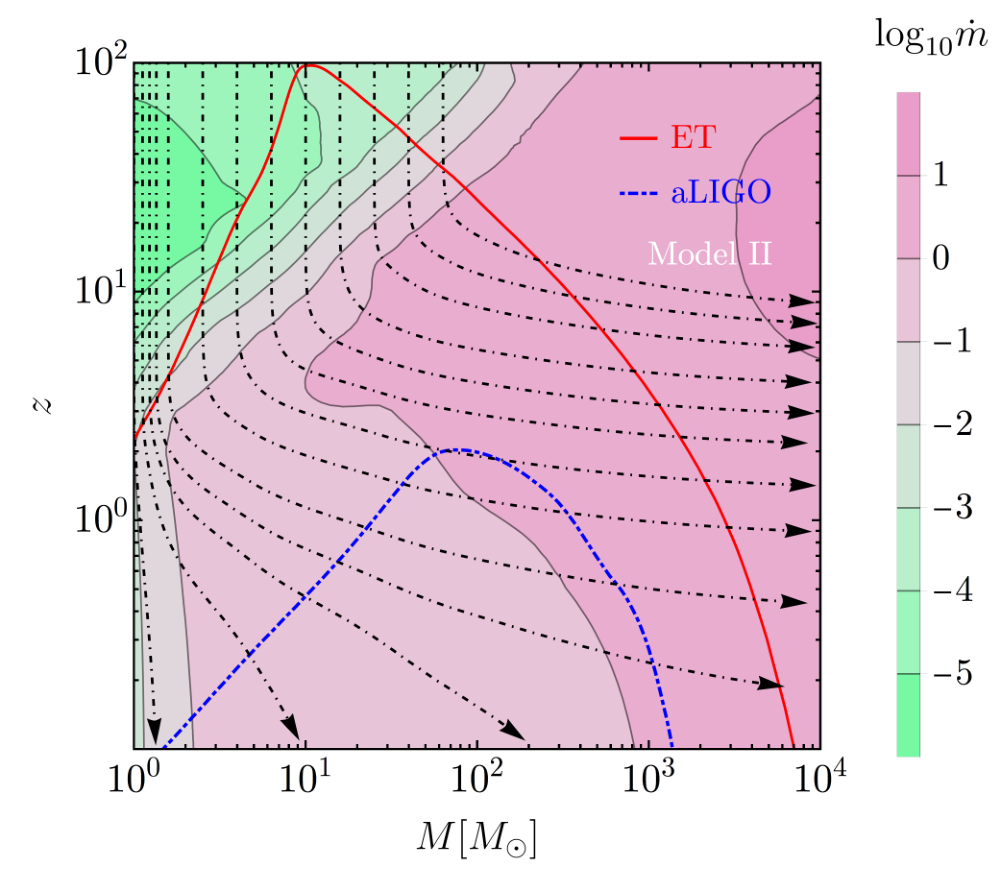
In Figs. 4 and 5 we present the evolution of the mass accretion rate (left panels) and spin (right panels) in the plane, starting from the initial conditions set at high redshifts (we assume initial conditions at ) for Model I and Model II, respectively. On the contour plots we also superimpose the curves representing the maximum distance current and future GW experiments like aLIGO and Einstein Telescope (ET) [65] may reach at a given redshift. We take such maximum distance to be the corresponding visible horizon.
In the mass range of interest no significant evolution of the mass (and, correspondingly, of the spin) takes place before redshift . This is due to the long time scales characterising the accretion compared to the age of the universe up to that epoch. After , PBHs masses start evolving rapidly for . In the left panels of Figs. 4 and 5 we show the trajectories (black dashed lines) that a PBH with a certain initial mass would follow during the cosmic history. Correspondingly, we observe that the spins of PBHs with masses , even if they start from an initial value at the percent level, make a rapid transition to extremality if, during its evolution, the system enters a region where . It is worth noting that the transition region is sensitive to the magnitude of and to the actual value of the redshift at which structure formation and reionization take place. In particular, increasing or delaying the reionization epoch would push the transition region to lower masses.
In the following, we describe in details the evolution of mass and spin after redshift separately for Model I and Model II. The implications regarding such a prediction for GW detections with aLIGO and ET are discussed in Sec. 4.2.
4.1.1 Model I
This model assumes a sharp decrease of the mass accretion rate after . As one can appreciate from Fig. 4 (left panel), each individual PBH starts following vertical trajectories in the plane after that redshift. This shows that the mass evolution is negligible in that region. Correspondingly, the spin stops evolving after that epoch, see right panel of Fig. 4. We note a correlation between low (high) values of the masses and low (high) spins, with a sharp transition around . More specifically, PBHs with masses below are non-spinning, whereas heavier PBHs can be nearly extremal up to redshift for , and even to higher redshifts for heavier PBHs, although that region will be outside the horizon of ET. One can notice that in this region high values of the spin are not reached for values of redshift higher than due to the large accretion time scales with respect to the age of the universe at that epoch.


4.1.2 Model II
This model assumes a sustained accretion after redshift . At variance with Model I, the evolution of the mass and spin proceeds after that redshift, with a significant increase also of the smaller masses.
The transition region between small and high values of the spin after redshift is pushed to higher masses respect to model I as now PBHs with those masses have never experienced a period of thin disk accretion. Also, for masses smaller than , the spherical accretion, while leaving unaffected, decreases the Kerr parameter , thus erasing any memory of the initial spin. We finally note that – in the region in which is bigger than unity – an extremal value of the spin is always rapidly attained. One can also appreciate that in this model PBHs within the aLIGO horizon are expected to be slowly spinning with small values of

4.2 Implications for GW events
Ultimately, we are interested in giving the prediction for the key observables which can be measured in GW coalescence events with current (LIGO/Virgo) and future (e.g., ET) detectors55 5 We are neglecting the possible effect of accretion during the coalescence as we expect the increase in velocity to happen only during the last stages of inspiral and thus at much smaller characteristic time scales..
In a merger event of two PBHs with masses and with a binary mass ratio defined as , and dimensionless spin vectors and , one can estimate the final spin of the PBH resulting from the merger as [66, 68, 67, 69]
| (4.1) |
with
| (4.2) |
in terms of the numerical parameters , , , and . Here is the symmetric mass ratio and
| (4.3) |
are the angles (at large separation) between the two spins and between each individual spin and the direction of the orbital angular momentum , respectively. The mass of the final PBH is [70]
| (4.4) |
where and are numerical coefficients.
The effect of the spin of the binary components mostly affects the gravitational waveform to leading post-Newtonian order through the effective spin parameter, defined as the mass weighted projection of the effective spin of the binary to the orbital angular momentum (see Eq. (1.1)),
| (4.5) |
where, being , the possible range of values is .66 6 The occurrence of merging events with highly-spinning components may also increase the stochastic GW background signal resulting from the coalescences, with a consequent change in the deduced bounds from its non-observation [71], see Ref. [72] for details about the radiated energy from a merging event in terms of the BHs spin.
The effective spins measured so far with GWs are affected by large uncertainties and are compatible to zero for almost all sources [3]. Only few high-mass events have been detected so far for which [4, 21, 20], although for two low-significance events – namely GW151216 and GW170403 – the measured value of is significantly affected by the prior on the spin angles [22]. Furthermore, future detections will provide measurements of the individual spins with accuracy [2], also alleviating the degeneracy between the individual spins and other binary parameters such as the mass ratio.
To obtain the probability distribution functions (PDFs) of the spin (4.1) and mass (4.4) of the merger remnant, along with the effective spin of the binary (4.5), one has to perform a statistical ensemble over the masses of the binary components and the relevant angles of the spin vectors. We have assumed a uniform distribution for the spin vectors orientations on a unit two-sphere [4, 28] and several shapes of the mass functions (see Appendix C) at the redshift of observation . Such shapes are assumed to result from the evolution of an initial mass function due to mass accretion, see Appendix D for details about this time evolution.
Results are shown in Fig. 6, where for simplicity we have assumed that both components of the binary have the same spin before merger, . We stress that the colour code used to plot the probability distributions corresponding to a particular spin , as shown in the legend, has been chosen to match the one used in Figs. 4 and 5 (right panels). In other words, one can identify the expected PDFs for the relevant parameters in each point of the parameter space of the contour plots by looking at the corresponding colour in Fig. 6. In particular, the distributions shown in Fig. 6 only depend on the value of the binary component spins at coalescence. They are therefore similar to those computed in other astrophysical scenarios [63, 28, 29]. However, there are crucial differences in our case. One is the effect that the value of the individual spins is correlated with the mass of the binary components and with the redshift at coalescence. Another one is the presence of a given PBH mass function.
The first column shows the PDFs for a monochromatic shape of the mass function, for which the mass ratio of the binary is , while the second and third columns show the result for more realistic and broader shapes of the mass distribution, namely a critical mass and lognormal with width , respectively, for which the mass ratio distribution is peaked at smaller values (see Appendices C and D for details about the mass functions).
Since the individual spins are isotropically oriented, the PDF for the effective spin parameter of the binary (first row) is peaked around the central value for small initial spins, maintaining the peak also for broader mass functions. However, for higher initial spins the distribution of is much broader for all choices of the mass function.
The PDF of the final spin (second row) is peaked at the value for low initial spins of the binary (since in this case the distribution is almost independent on the values of the spins angles), and the distribution becomes broader for bigger values of the PBH spins before the merger. For broader mass functions the PDF tends to become broader (see panels of Fig. 6 from left to right).
Finally, the probability distribution for the final mass peaks at the value for low initial spins; the peak values decrease for broader mass functions, and has a flatter shape for higher spins. One can also notice how the distribution tends to be asymmetric with respect to the centre for broader mass functions.
In Figs. 7, 8, and 9 we provide the confidence intervals for given mass at 68% (), 95% () and 99% () CL for the final mass, spin, and for the effective spin parameter of the merging binary. We construct these distributions by fixing the mass ratio77 7 The distribution of the mass ratio for different mass functions is discussed in Appendix D, see Fig. 12. ( in Fig. 7, in Fig. 8, and in Fig. 9, respectively) and, for each value of redshift and of the mass of the primary component of the binary, we draw the individual spin directions from an isotropic distribution whereas the spin magnitudes are obtained as from the right panels of Figs. 4 and 5 for Model I and Model II, respectively. The probabilities are evaluated at a fixed redshift for both Model I and Model II for the left panels and at for Model II for the right panels. We have also reported the data (with error bars) corresponding to the GW events detected so far in the first two observation runs of LIGO and Virgo (only for the plots with and which are consistent with the observed mass ratios). In particular, the blue data points refer to events with high statistical significance [4], whereas green and red data points refer to the events discovered in Refs. [21, 20], which have a lower statistical significance. The red data points refer to GW151216 and GW170403, for which the measured value of is significantly affected by the priors, in particular whether one assumes a uniform prior on or an isotropic distribution for the directions of the individual spins with uniform magnitude of the latter [22]. The red and green data points in Fig. 7 refer to the former assumption.
For Model I the results in Fig. 7 show the general tendency of having peaked distributions for masses smaller than and broader ones for bigger masses once the transition from low to high spins has been reached, see Figs. 4 and 5 for details on the transition. Even though we have chosen (left panels), such a tendency is maintained for all redshifts smaller than . Interestingly, especially for (for only low mass data and the corresponding values of the final spin are excluded as one can see from Fig. 8), the predicted distributions in case of accreting PBHs are consistent with the observed distribution of the GW events detected so far [73], especially when including those obtained in Refs. [21, 20], which tend to have large effective spin for some high-mass binaries. It is harder to predict such distribution in the case of binaries of astrophysical origin, although binaries formed in stellar clusters by dynamical capture might have larger for larger total masses [23, 74]. For example, the predicted distribution in this case is in tension with a measurement and such as that reported in Ref. [21].
For Model II one observes a similar behaviour for all the probabilities of the three parameters, but at higher redshift (we stress that the left and right panels of Figs. (7-9) refer to and , respectively). As previously discussed, for Model II the effect of accretion on the spin in the present epoch for the range of masses of interest is small, which explains why in the left panels of Figs. (7-9) () the distributions for Model II appear as thin curves on the scale of the plots. In the right panels we have instead chosen the representative redshift , which corresponds to a transition mass , in order to highlight the tendency in the probability. In Fig. 8 the same tendency shows up with an additional transition point at higher values of due to the crossing point from low to high spins of the second mass .
For low mass ratios, in Fig. 9, there is a general tendency for which the mass and the spin of the lighter component of the binary play a minor role in the determination of the spin parameters. In particular, is mainly affected by and attains values close to zero and for the lightest and largest mass, respectively (the sign depending upon the spin orientation). This tendency manifests itself by having a much broader confidence interval in the high mass portion of Fig. 9. The final spin of the remnant BH is mainly inherited by the primary constituent of mass of the binary, and for small initial spins we find in the limit of small from Eq. (4.1). This explains the shift of towards zero for smaller mass ratios. On the other hand, the distribution shifts towards higher values of in the case of a highly spinning primary, for small . Finally, the rescaled final mass tends towards unity as .
Overall, the effect of having higher binary-component spins is to make the distributions of , , and broader (see Fig. 6). Thus, our main results are robust against the value of the maximum spin reached through accretion, in particular they would be qualitatively the same also if the maximum value is , as suggested by magnetohydrodynamic simulations of relatively thick disks [64]. In this case we expect the distributions to be slightly less broad.
5 Conclusions
In this paper we have discussed the cosmological evolution of the mass and spin of PBHs. Our results can be relevant in two contexts:
- •
For the merger events detected so far by LIGO-Virgo, the effective spin parameter of the binary is compatible to zero, except possibly for few high-mass events [3, 4, 21, 20, 22]. We have shown that a primordial origin of these BH binaries could naturally explain this distribution, especially in the likely scenario in which accretion is quenched at due to structure formation [41]. Indeed, due to the redshift dependence of the accretion rate, PBHs with masses below are likely non-spinning at any redshift, whereas heavier BHs can be nearly extremal up to redshift , resulting in a broader distribution of the effective spin parameter, which is compatible with the observed distribution of the GW events detected so far. On the contrary, it is more challenging to explain such distribution and - correlation in the case of binaries of astrophysical origin [23].
- •
Current bounds on PBH abundance assume that the mass distribution at the present epoch is the same as that at formation in the early universe. We have shown that accretion might significantly modify the mass and spin distributions in a redshift-dependent fashion. The implications of this effect for current constraints on PBHs will be discussed in a forthcoming work [46].
Upcoming results from LIGO-Virgo third observation run might reinforce or weaken these predictions, in particular whether light binaries (mass of the binary components ) can have large effective spin parameter or not.
Future detections will provide measurements not only of the effective spin of the binary, but also of the individual spins, with accuracy [2]. This will allow to constrain the primordial formation scenario more accurately and possibly distinguish between different formation mechanisms and different accretion models. Indeed, the physics of accretion in the early universe is very rich [40, 41]. A natural extension of our work would be to refine the accretion model, for example considering also (relatively) thick accretion disks and other models of the accretion flow. Overall, our results suggest that it would be crucial to correlate the mass and spin distributions with the redshift of the source, since the transition between non-spinning and highly-spinning BHs occurs at redshift . This will be possible with future GW detectors, such as ET, that will detect binary BHs up [65].
Acknowledgments
We thank E. Barausse, V. Desjacques, F. Khnel, M. Maggiore, M. Ricotti, H. Veerme and A. Zimmerman for interesting discussions, and E. Berti for useful comments on the draft. V.DL., G.F. and A.R. are supported by the Swiss National Science Foundation (SNSF), project The Non-Gaussian Universe and Cosmological Symmetries, project number: 200020-178787. P.P. acknowledges financial support provided under the European Union’s H2020 ERC, Starting Grant agreement no. DarkGRA–757480, under the MIUR PRIN and FARE programmes (GW-NEXT, CUP: B84I20000100001), and support from the Amaldi Research Center funded by the MIUR program ‘Dipartimento di Eccellenza” (CUP: B81I18001170001).
Appendix A Binary merger rates
In this Appendix we review the formation of PBH binaries and their related merging rate, see Ref. [10] for a review. There are two main formation mechanisms for PBH binaries, one taking place in the early universe, especially before matter-radiation equality, and the other taking place in the late time universe in the present-day halos. For simplicity, we provide the estimates for equal masses binaries.
A.1 Early-time PBH binaries
A pair of neighboring PBHs of masses separated by a physical distance can decouple from the Hubble flow provided that their gravitational interaction is strong enough, i.e. , where represents the background cosmic energy density. Expressing the quantities with respect to the ones at the matter-radiation equality , one finds that the decoupling occurs at if
| (A.1) |
where we denoted with the fraction of PBHs in DM at that time, and the PBH physical mean separation reads
| (A.2) |
Eq. (A.1) shows that the characteristic formation redshift is of the order for the masses and considered [47].
The initial infall motion of the PBHs can be affected by the surrounding, and especially the closest, PBHs, which can exert tidal forces and give angular momentum to the system, forming therefore a binary. The semi-major axis and the eccentricity of the binary are given by
| (A.3) |
where is the physical distance to the third PBH at . In the following we will assume [75, 76] (for a more precise quantitative estimate of these coefficients see Ref. [77]). Imposing the geometrical condition one gets an upper bound on the eccentricity as
| (A.4) |
Assuming a uniform probability distribution for both and in three dimensional space and converting it in terms of and , one obtains
| (A.5) |
Once the PBHs form a binary, their distance gradually shrinks due to the energy loss through GWs radiation and eventually merge with a coalescence time given by [78, 79]
| (A.6) |
We can convert the probability distribution above in terms of the coalescence time and eccentricity, and then integrate over for fixed time . The probability that the coalescence occurs in the time interval can be then connected to the merger rate through the PBH number density as (see also [71, 80, 81])
| (A.7) |
where and . The corresponding merging rate is shown in Fig. 10.
A.2 Late-time PBH binaries
A second mechanism of formation of PBH binaries can take place in the present-day halos [82, 5]. If a PBH moving at a given velocity passes close to another PBH, the energy loss due to the sudden GW emission can make the former loose its kinetic energy becoming bound to the latter. The energy loss during the encounter can be estimated to be
| (A.8) |
where is the periastron. Using the Newtonian approximation, for which the impact parameter is , one finds the cross section for a binary formation
| (A.9) |
Once formed, such a binary can merge in less than the age of the universe. The merger rate for a halo of mass can be computed as
| (A.10) |
where identifies the virial radius, is the PBH local density profile (typically taken to be the Navarro-Frenk-White profile) and the brackets stand for the mean value of the combination computed using the Maxwell-Boltzmann velocity distribution. Finally, the total merger rate is found to be
| (A.11) |
where is the minimum halo mass [10]. The result is sensitive to the mass function which can be estimated using Press-Schechter formalism [83] or based on numerical simulations as in Refs. [84, 85]. As shown in Fig. 10, the final merger rate is orders of magnitude lower than its early universe counterpart, but one should take into account various uncertainties. Furthermore, for future experiments like ET which will have a much larger statistics, late-time universe binary mergers will be relevant.
Appendix B Mass accretion rate
In the case of a dark halo clothing, we need to take into account the dark halo mass given in Eq. (2.6) and, if the typical size of the halo is smaller than the Bondi radius, then the accretion rate is the same as the one for a PBH of point mass . We can define the parameter
| (B.1) |
Different behaviors occurs when or . In the former case the dark halo behaves the same as a point mass in terms of accretion rate, sonic radius and viscosity, with accretion rate given by [41]
| (B.2) |
where
| (B.3) |
in terms of the sonic radius
| (B.4) |
and the gas viscosity parameter given by
| (B.5) |
as a function of the redshift, the PBH mass, effective velocity, and ionization fraction of the cosmic gas .
If one has instead to correct the quantities with respect to the naked case as
| (B.6) |
where and
| (B.7) |
The proper motion of PBHs strongly affects the dynamics of the accretion process and depends on the amplitude of the inhomogeneities of the DM and baryon fluids. Following Ref. [41], one can estimate the relative velocity of PBHs with respect to the accreting baryonic matter assuming PBHs to behave like DM particles and identifying two main regimes of interest, the linear and non-linear regime.
In the linear regime before the decoupling redshift , the Silk damping acts suppressing the growth of inhomogeneities on small scales, such that the PBH peculiar velocity is of order of the gas sound speed; for , the gas flow lags behind the DM with a relative velocity , such that the PBH peculiar velocity follows a Maxwellian distribution with variance and has expectation value given by [41]
| (B.8) |
in terms of the Mach number . Here the scenario A refers to a low efficient accretion rate, , characterised by a spherical geometry, while scenario B refers to an efficient accretion rate, , which supports the presence of an accretion disk, see Sec. 2.
In the non-linear regime, the non-linear perturbations (halos) can prevent PBHs to accrete gas from the intergalactic medium, since they make PBHs fall in their potential wells with an enhanced velocity, which leads to a huge suppression of the gas accretion rate for an increasingly large fraction of the PBH population. To account for this possibility, in the main text we assumed two opposite and extreme models, dubbed as Model I (in which accretion at is suppressed) and Model II (in which accretion is sustained also when ).
Appendix C Effects of second-generation mergers and PBH mass functions
The analysis presented in the main text ignores the possibility of second-generation mergers. Namely, a PBH binary might merge into a new BH which, at a later time, might undergo a further coalescence with another PBH, forming a new PBH binary which is eventually detected. We report here the formalism to compute the secondary mergers rates following the approach in Ref. [86, 87]88 8 The analysis we adopt neglects the suppression factor on the merging rates due to the disruption of the binaries from the surrounding PBHs, which is found to be effective only for [80, 88]. Taking into account this effect would make the conclusion of this Appendix slightly stronger..
In the following we will assume that the fraction of PBHs as DM, , is bigger than a critical value , above which the effects of the linear density perturbations are negligible on the merger rate of PBH binaries. The critical value reads
| (C.1) |
and is at most of order for the relevant range of masses at the present time . Here is the reference mass associated to the scale re-entering the horizon.
We define the mass function identifying the fraction of PBHs with mass in the range as
| (C.2) |
normalised such that
| (C.3) |
The fraction of the present average number density of PBHs with mass with respect to the total average is given by the expression
| (C.4) |
and the fraction of PBHs that have undergone a merging event before the time is given by [86]
| (C.5) |
where all the dependence on the shape of the mass function is given by the adimensional factor
| (C.6) |
where and . The fraction of PBHs that have merged in a second-merger process at time is instead given by [86]
| (C.7) |
in terms of the factor
| (C.8) |
The conditional probability that PBHs which have merged are the results of a second-merger process at time is given by
| (C.9) |
Typically, various shapes of the mass fraction are considered in literature, corresponding to the most common formation scenarios of PBHs. In the following we will consider a critical, spiky, lognormal, and power-law mass functions.
- •
- •
Monochromatic mass function: PBHs which have a monochromatic mass function are distributed as
(C.12) i.e. they have all the same mass . The resulting value for the rescaled merger fraction is . This case is the simplest configuration but it is unrealistic since even a monochromatic power spectrum of curvature perturbations gives rise to a larger mass function (i.e. the “critical scaling mass function” presented above) due to the dynamics of the critical collapse.
- •
Lognormal mass function: this represents a frequent parametrisation which describes the case of a PBHs population arising from a symmetric peak in the primordial power spectrum, see for example Ref. [91] and references therein, being
(C.13) The resulting value for the rescaled merger fraction is , depending on the width of the distribution .
- •
Power-law mass function: which is typically obtained when considering the time evolution for models with a broad power spectrum of the curvature perturbations, see Ref. [92],
(C.14) The resulting value for the rescaled merger fraction is .
In Fig. 11 we plotted in terms of the total mass of the observed binary and the redshift assuming a certain value for the fraction of PBHs as DM . We superimpose the curves representing the horizon at which aLIGO and ET experiments will be able to detect a merger at that total mass and redshift, assuming equal-mass and non-spinning binaries, see Refs. [93, 94]. The plotted results are found assuming a critical scaling mass function. Other mass functions typically used in literature would give rise to corrections to the result.


One can conclude that only a tiny fraction of BHs detectable through their merger at aLIGO or ET have suffered a previous merger. This implies that the spin of each binary component is the one at primordial formation, plus possibly its accretion contribution, as discussed in the main text.
Appendix D The evolution of the mass function
In this appendix we discuss how the mass function changes when the mass evolution is taken into account. To give a quantitative estimate of this effect we will consider some of the mass functions analysed in the previous appendix, which are summarised in the left panel of Fig. 12. The resulting distribution of the mass ratio for a random pair of masses (, ) in each case is plotted in the right panel of Fig. 12. One can notice how peaked mass functions give a distribution for the mass ratio peaked close to unity, while broader mass functions favour mass ratios closer to zero.
The evolution of the mass function can be computed analytically once the mass evolution is taken into account. Following the evolution of the mass accretion rate (see Fig. 4 for Model I and Fig. 5 for Model II) one can start with a certain mass at high redshift and evolve it into a different mass as
| (D.1) |
Correspondingly, defining as the mass function at the formation time, the resulting mass function at redshift will be
| (D.2) |
One can check explicitly that the unitary normalisation is maintained.
Fig. 13 shows the evolution of the mass function for Model I (top panels) and Model II (bottom panels), for the choices of a critical and lognormal shape at the formation time. As the evolution proceeds, the height of the mass function decreases with a consequent increase of the tail of the distribution due to the effect of the accretion processes, even though the peak is maintained at almost the same position in the mass range.
References
- [1] B. P. Abbott et al. [LIGO Scientific and Virgo Collaborations], Phys. Rev. Lett. 116, no. 6, 061102 (2016) [gr-qc/1602.03837].
- [2] B. P. Abbott et al. [LIGO Scientific and Virgo Collaborations], Phys. Rev. X 6, no. 4, 041015 (2016) Erratum: [Phys. Rev. X 8, no. 3, 039903 (2018)] [gr-qc/1606.04856].
- [3] B. P. Abbott et al. [LIGO Scientific and Virgo Collaborations], Astrophys. J. 882 (2019) no.2, L24 [astro-ph.HE/1811.12940].
- [4] B. P. Abbott et al. [LIGO Scientific and Virgo Collaborations], Phys. Rev. X 9, no. 3, 031040 (2019) [astro-ph.HE/1811.12907].
- [5] S. Bird, I. Cholis, J. B. Muñoz, Y. Ali-Haïmoud, M. Kamionkowski, E. D. Kovetz, A. Raccanelli and A. G. Riess, Phys. Rev. Lett. 116, no. 20, 201301 (2016) [astro-ph.CO/1603.00464].
- [6] B. J. Carr, K. Kohri, Y. Sendouda and J. Yokoyama, Phys. Rev. D 81, 104019 (2010) [astro-ph.CO/0912.5297].
- [7] B. Carr, F. Kuhnel and M. Sandstad, Phys. Rev. D 94, no. 8, 083504 (2016) [astro-ph.CO/1607.06077].
- [8] S. Blinnikov, A. Dolgov, N. K. Porayko and K. Postnov, JCAP 1611, 036 (2016) [astro-ph.HE/1611.00541].
- [9] J. García-Bellido, J. Phys. Conf. Ser. 840, no. 1, 012032 (2017) [astro-ph.CO/1702.08275].
- [10] M. Sasaki, T. Suyama, T. Tanaka and S. Yokoyama, Class. Quant. Grav. 35, no. 6, 063001 (2018) [astro-ph.CO/1801.05235].
- [11] L. Barack et al., Class. Quant. Grav. 36, no. 14, 143001 (2019) [gr-qc/1806.05195].
- [12] B. Carr, K. Kohri, Y. Sendouda and J. Yokoyama, [astro-ph.CO/2002.12778].
- [13] P. Ivanov, P. Naselsky and I. Novikov, Phys. Rev. D 50, 7173 (1994).
- [14] J. García-Bellido, A.D. Linde and D. Wands, Phys. Rev. D 54 (1996) 6040 [astro-ph/9605094].
- [15] P. Ivanov, Phys. Rev. D 57, 7145 (1998) [astro-ph/9708224].
- [16] Y. Ali-Haïmoud, Phys. Rev. Lett. 121, no. 8, 081304 (2018) [astro-ph.CO/1805.05912].
- [17] V. Desjacques and A. Riotto, Phys. Rev. D 98, no. 12, 123533 (2018) [astro-ph.CO/1806.10414].
- [18] G. Ballesteros, P. D. Serpico and M. Taoso, JCAP 1810, 043 (2018) [astro-ph.CO/1807.02084].
- [19] A. Moradinezhad Dizgah, G. Franciolini and A. Riotto, JCAP 1911, no. 11, 001 (2019) [astro-ph.CO/1906.08978].
- [20] T. Venumadhav, B. Zackay, J. Roulet, L. Dai and M. Zaldarriaga, [astro-ph.HE/1904.07214].
- [21] B. Zackay, T. Venumadhav, L. Dai, J. Roulet and M. Zaldarriaga, Phys. Rev. D 100, no. 2, 023007 (2019) [astro-ph.HE/1902.10331].
- [22] Y. Huang et al., [gr-qc/2003.04513].
- [23] M. Safarzadeh, W. M. Farr and E. Ramirez-Ruiz, [gr-qc/2001.06490].
- [24] L. Blanchet, Living Rev. Rel. 17, 2 (2014) [gr-qc/1310.1528].
- [25] D. Gerosa, M. Kesden, E. Berti, R. O’Shaughnessy and U. Sperhake, Phys. Rev. D 87, 104028 (2013) [gr-qc/1302.4442].
- [26] D. Gerosa, E. Berti, R. O’Shaughnessy, K. Belczynski, M. Kesden, D. Wysocki and W. Gladysz, Phys. Rev. D 98, no. 8, 084036 (2018) [astro-ph.HE/1808.02491].
- [27] C. L. Rodriguez, M. Zevin, C. Pankow, V. Kalogera and F. A. Rasio, Astrophys. J. 832, no. 1, L2 (2016) [astro-ph.HE/1609.05916].
- [28] D. Gerosa and E. Berti, Phys. Rev. D 95, no. 12, 124046 (2017) [gr-qc/1703.06223].
- [29] M. Fishbach, D. E. Holz and B. Farr, Astrophys. J. 840, no. 2, L24 (2017) [astro-ph.HE/1703.06869].
- [30] W. M. Farr, S. Stevenson, M. Coleman Miller, I. Mandel, B. Farr and A. Vecchio, Nature 548, 426 (2017) [astro-ph.HE/1706.01385].
- [31] B. Farr, D. E. Holz and W. M. Farr, Astrophys. J. 854, no. 1, L9 (2018) [astro-ph.HE/1709.07896].
- [32] K. Belczynski et al., [astro-ph.HE/1706.07053].
- [33] S. Vitale, D. Gerosa, C. J. Haster, K. Chatziioannou and A. Zimmerman, Phys. Rev. Lett. 119, no. 25, 251103 (2017) [gr-qc/1707.04637].
- [34] M. Mirbabayi, A. Gruzinov and J. Noreña, [astro-ph.CO/1901.05963].
- [35] V. De Luca, V. Desjacques, G. Franciolini, A. Malhotra and A. Riotto, JCAP 05 (2019), 018 [astro-ph.CO/1903.01179].
- [36] E. Cotner and A. Kusenko, Phys. Rev. D 96 (2017) no.10, 103002 [astro-ph.CO/1706.09003].
- [37] T. Harada, C. M. Yoo, K. Kohri and K. I. Nakao, Phys. Rev. D 96, no. 8, 083517 (2017) Erratum: [Phys. Rev. D 99, no. 6, 069904 (2019)] [gr-qc/1707.03595].
- [38] E. Berti and M. Volonteri, Astrophys. J. 684, 822 (2008) [astro-ph/0802.0025].
- [39] N. Fernandez and S. Profumo, JCAP 1908, 022 (2019) [astro-ph.HE/1905.13019].
- [40] M. Ricotti, Astrophys. J. 662, 53 (2007) [astro-ph/0706.0864].
- [41] M. Ricotti, J. P. Ostriker and K. J. Mack, Astrophys. J. 680, 829 (2008) [astro-ph/0709.0524].
- [42] P. Pani and A. Loeb, Phys. Rev. D 88, 041301 (2013) [astro-ph.CO/1307.5176].
- [43] R. Brito, V. Cardoso and P. Pani, Lect. Notes Phys. 906, pp.1 (2015) [gr-qc/1501.06570].
- [44] J. P. Conlon and C. A. R. Herdeiro, Phys. Lett. B 780, 169 (2018) [astro-ph.HE/1701.02034].
- [45] A. Dima and E. Barausse, [gr-qc/2001.11484].
- [46] V. De Luca, G. Franciolini, P. Pani, A. Riotto, to appear (2020).
- [47] Y. Ali-Haïmoud, E. D. Kovetz and M. Kamionkowski, Phys. Rev. D 96, no. 12, 123523 (2017) [astro-ph.CO/1709.06576].
- [48] Y. Ali-Haïmoud and M. Kamionkowski, Phys. Rev. D 95, no. 4, 043534 (2017) [astro-ph.CO/1612.05644].
- [49] B. Horowitz, [astro-ph.CO/1612.07264].
- [50] V. Poulin, P. D. Serpico, F. Calore, S. Clesse and K. Kohri, Phys. Rev. D 96, no. 8, 083524 (2017) [astro-ph.CO/1707.04206].
- [51] P. D. Serpico, V. Poulin, D. Inman and K. Kohri, [astro-ph.CO/2002.10771].
- [52] S. L. Shapiro and S. A. Teukolsky Black holes, white dwarfs, and neutron stars: The physics of compact objects (Wiley, 1983).
- [53] K. J. Mack, J. P. Ostriker and M. Ricotti, Astrophys. J. 665, 1277 (2007) [astro-ph/0608642].
- [54] J. Adamek, C. T. Byrnes, M. Gosenca and S. Hotchkiss, Phys. Rev. D 100 (2019) no.2, 023506 [astro-ph.CO/1901.08528].
- [55] J. R. Rice and B. Zhang, JHEAp 13-14, 22 (2017) [astro-ph.HE/1702.08069].
- [56] E. Barausse, V. Cardoso and P. Pani, Phys. Rev. D 89 (2014) no.10, 104059 [gr-qc/1404.7149].
- [57] G. Hütsi, M. Raidal and H. Veermäe, Phys. Rev. D 100, no. 8, 083016 (2019) [astro-ph.CO/1907.06533].
- [58] D. Inman and Y. Ali-Haïmoud, Phys. Rev. D 100 (2019) no.8, 083528 [astro-ph.CO/1907.08129].
- [59] J. M. Bardeen, J. Bond, N. Kaiser and A. Szalay, Astrophys. J. 304 (1986), 15-61
- [60] J. M. Bardeen, W. H. Press and S. A. Teukolsky, Astrophys. J. 178, 347 (1972).
- [61] K. S. Thorne, Astrophys. J. 191 (1974), 507-520
- [62] R. Brito, V. Cardoso and P. Pani, Class. Quant. Grav. 32, no. 13, 134001 (2015) [gr-qc/1411.0686].
- [63] M. Volonteri, P. Madau, E. Quataert and M. J. Rees, Astrophys. J. 620, 69 (2005) [astro-ph/0410342].
- [64] C. F. Gammie, S. L. Shapiro and J. C. McKinney, Astrophys. J. 602, 312 (2004) [astro-ph/0310886].
- [65] S. Hild et al., Class. Quant. Grav. 28, 094013 (2011) [gr-qc/1012.0908].
- [66] E. Barausse and L. Rezzolla, Astrophys. J. 704, L40 (2009) [gr-qc/0904.2577].
- [67] E. Barausse, Mon. Not. Roy. Astron. Soc. 423, 2533 (2012) [astro-ph.CO/1201.5888].
- [68] M. Kesden, U. Sperhake and E. Berti, Phys. Rev. D 81, 084054 (2010) [astro-ph.GA/1002.2643].
- [69] F. Hofmann, E. Barausse and L. Rezzolla, Astrophys. J. 825 (2016) no.2, L19 [gr-qc/1605.01938].
- [70] W. Tichy and P. Marronetti, Phys. Rev. D 78 (2008), 081501 [gr-qc/0807.2985].
- [71] M. Raidal, V. Vaskonen and H. Veermäe, JCAP 1709, 037 (2017) [astro-ph.CO/1707.01480].
- [72] D. A. Hemberger, G. Lovelace, T. J. Loredo, L. E. Kidder, M. A. Scheel, B. Szilágyi, N. W. Taylor and S. A. Teukolsky, Phys. Rev. D 88, 064014 (2013) [gr-qc/1305.5991].
- [73] A. D. Gow, C. T. Byrnes, A. Hall and J. A. Peacock, JCAP 01 (2020) no.01, 031 [astro-ph.CO/1911.12685].
- [74] M. Safarzadeh, [astro-ph.HE/2003.02764].
- [75] T. Nakamura, M. Sasaki, T. Tanaka and K. S. Thorne, Astrophys. J. 487, L139 (1997) [astro-ph/9708060].
- [76] M. Sasaki, T. Suyama, T. Tanaka and S. Yokoyama, Phys. Rev. Lett. 117, no. 6, 061101 (2016) Erratum: [Phys. Rev. Lett. 121, no. 5, 059901 (2018)] [astro-ph.CO/1603.08338].
- [77] K. Ioka, T. Chiba, T. Tanaka and T. Nakamura, Phys. Rev. D 58, 063003 (1998) [astro-ph/9807018].
- [78] P. C. Peters and J. Mathews, Phys. Rev. 131, 435 (1963).
- [79] P. C. Peters, Phys. Rev. 136, B1224 (1964).
- [80] M. Raidal, C. Spethmann, V. Vaskonen and H. Veermäe, JCAP 02 (2019), 018 [astro-ph.CO/1812.01930].
- [81] S. Wang, T. Terada and K. Kohri, Phys. Rev. D 99, no. 10, 103531 (2019) [astro-ph.CO/1903.05924].
- [82] G. D. Quinlan and S. L. Shapiro, Astrophys. J. 343, 725 (1989)
- [83] W. H. Press and P. Schechter, Astrophys. J. 187, 425 (1974).
- [84] J. L. Tinker, A. V. Kravtsov, A. Klypin, K. Abazajian, M. S. Warren, G. Yepes, S. Gottlober and D. E. Holz, Astrophys. J. 688, 709 (2008) [astro-ph/0803.2706].
- [85] A. Jenkins, C. S. Frenk, S. D. M. White, J. M. Colberg, S. Cole, A. E. Evrard, H. M. P. Couchman and N. Yoshida, Mon. Not. Roy. Astron. Soc. 321, 372 (2001) [astro-ph/0005260].
- [86] L. Liu, Z. K. Guo and R. G. Cai, Eur. Phys. J. C 79 (2019) no.8, 717 [astro-ph.CO/1901.07672].
- [87] Y. Wu, [astro-ph.CO/2001.03833].
- [88] V. Vaskonen and H. Veermäe, Phys. Rev. D 101, no. 4, 043015 (2020) [astro-ph.CO/1908.09752].
- [89] J. C. Niemeyer and K. Jedamzik, Phys. Rev. Lett. 80, 5481 (1998) [astro-ph/9709072].
- [90] J. Yokoyama, Phys. Rev. D 58, 107502 (1998) [gr-qc/9804041].
- [91] B. Carr, M. Raidal, T. Tenkanen, V. Vaskonen and H. Veermäe, Phys. Rev. D 96, no. 2, 023514 (2017) [astro-ph.CO/1705.05567].
- [92] V. De Luca, G. Franciolini and A. Riotto, [astro-ph.CO/2001.04371].
- [93] B. S. Sathyaprakash et al., [astro-ph.HE/1903.09260].
- [94] M. Maggiore et al., [astro-ph.CO/1912.02622].