Radio view of a broad-line Type Ic supernova ASASSN-16fp2020Radio view of a broad-line Type Ic supernova ASASSN-16fp–References
Abstract
We present extensive radio observations of a Type Ic supernova, ASASSN-16fp. Our data represents the lowest frequency observations of the SN beyond 1000 days with a frequency range of GHz and a temporal range of 8 to 1136 days post-explosion. The observations are best represented by a model of synchrotron emission from a shocked circumstellar shell initially suppressed by synchrotron self-absorption. Assuming equipartition of energy between relativistic particles and magnetic fields, we estimate the velocity and radius of the blast wave to be and cm respectively at 8 days post-explosion. We infer the total internal energy of the radio-emitting material evolves as 0.37 (t/t0)0.65 erg. We determine the mass-loss rate of the progenitor star to be at various epochs post-explosion, consistent with the mass-loss rate of Galactic Wolf-Rayet stars. The radio light curves and spectra show a signature of density enhancement in the CSM at a radius of cm from the explosion center.
Keywords:
Supernovae: general – supernovae: ASASSN-16fp – radiation mechanisms: non-thermal – circumstellar matter – radio continuum: general1 Introduction
Core-collapse Supernovae (SNe) show considerable diversity in their observational signatures. They are classified into various sub-classes based on the distinct features in the optical light curve and spectra. Type Ib/c SNe (hereafter SNe Ib/c) is a sub-class of core-collapse SNe that shows no hydrogen lines in their optical spectra (Filippenko 1997). In a volume-limited sample of all core-collapse SNe, Type Ibc comprises of 22% of the sample (Smith et al. 2011) and hence is an important mode of massive stellar death. Among SNe Ib/c , SNe Ib is characterized by the presence of helium lines in their spectra whereas SNe Ic does not show any helium lines (or very weak helium lines). Some SNe Ic show broad absorption lines in their optical spectra and they are called broad-lined SNe Ic (Valenti et al. 2008, SNe Ic-BL;). SNe Ic-BL are understood to have higher energy than typical SNe Ib/c (Foley et al. 2003; Valenti et al. 2008). A sub-population of SNe Ic-BL are associated with Gamma-ray bursts (GRBs), some are SN 1998bw/GRB 980425 (Galama et al. 1998; Pian et al. 2000), SN 2003dh/GRB 030329 (Berger et al. 2003; Hjorth et al. 2003; Mazzali et al. 2003; Frail et al. 2005), SN 2016jca/GRB 161219B (D’Ai et al. 2016; de Ugarte Postigo et al. 2016; Ashall et al. 2017; Alexander et al. 2016; Nayana & Chandra 2016).
The progenitors of SNe Ib/c are understood to be massive stars that have lost their hydrogen and/or helium layers before the core-collapse. The two popular progenitor models are the following. A single massive star that lost its outer hydrogen and/or helium envelope via strong stellar winds (Ensman, & Woosley 1988) or a massive star in a binary system where the outer stellar layers are stripped off due to binary interactions (Woosley et al. 1995; Yoon et al. 2010; Yoon 2015). There is one direct detection of the progenitor of this class in the case of SN PTF13bv (Cao et al. 2013, a Type Ib SN;). The zero-age-main sequence (ZAMS) mass of the progenitor was determined to be 30 from broad-band magnitudes (Cao et al. 2013; Groh et al. 2013). Alternatively the progenitor colors can also be reproduced in a binary model with ZAMS mass combinations of either 20 + 19 or 10 + 8 (Bersten et al. 2014; Eldridge et al. 2015). The direct detections still lack the sensitivity to discriminate the single star and binary progenitor models. Other than this one detection, there is no direct evidence of progenitor stars of this class. Thus the progenitor scenario and the mass range of progenitor stars of SNe Ibc is still an open problem. Any information about the nature of the progenitor system via indirect probes is important.
Radio emission from the hydrodynamical interaction of supernova (SN) with the circumstellar medium (CSM) is an important probe to study the progenitor properties and immediate CSM (Chevalier 1982b). Radio observations and modeling can constrain various physical parameters like the mass-loss rate of the progenitor star, the radius of the blast wave, the post-shock magnetic field, and CSM density. The density of the CSM will be different for single mass progenitors and binary progenitors. A single Wolf-Rayet (WR) star will have a wind stratified media around it (Chu 2002) whereas a binary system is likely to have a disrupted CSM due to the outflows in a common envelope phase (Podsiadlowski 1992). Radio light curves probe the density structure of the CSM and can discriminate between the two progenitor scenarios.
In this paper, we present extensive radio observations of an SN Ic-BL, ASASSN-16fp over a frequency range of GHz and a temporal range of 8 to 1136 years post-explosion. We model the radio observation as synchrotron emission from the SN interaction with the CSM created by a steady stellar wind from the progenitor star (Chevalier 1982a; Chevalier 1982b). We derive the mass-loss rate of the progenitor star and blast wave parameters at multiple epochs of the SN evolution. We also compare the properties of ASASSN-16fp with other SNe Ib/c.
2 ASASSN-16fp
ASASSN-16fp was discovered by the All-sky automated survey for the supernovae (ASAS-SN) team (Holoien et al. 2016) on 2016 May 27.6 (UT) in the nearby galaxy UGC 11868 with an apparent magnitude of 15.7 (V-band). The distance towards the SN is Mpc (from NED). The SN was initially classified as a SN Ic-BL (Elias-Rosa et al. 2016) and later as a transitional SN between SNe Ib and SNe Ic-BL due to the presence of He lines in the early optical spectrum (Yamanaka et al. 2017). The date of explosion of ASASSN-16fp was estimated to be 2016 May 24.5 (UT) by extrapolating the rising part of the optical light curve (Yamanaka et al. 2017). Kumar et al. 2018 carried out optical follow-up observations of ASASSN-16fp during the photospheric phase (-10 to +33 days with respect to the B band maximum) and presented the light curve and low resolution spectra. Kumar et al. 2018 estimated the date of explosion to be 2016 May 25.9 (UT) by fitting the good cadence data points from the pre-maximum phase. The last non-detection of ASASSN-16fp was on 2016 May 21.5 (UT) (Holoien et al. 2016). Thus both the explosion dates derived by Yamanaka et al. 2017 and (Kumar et al. 2018) are consistent with a maximum uncertainty of t = May = 6.1. In this work, we adopt the date of explosion to be 2016 May 25.9 (UT).
Prentice et al. 2018 presented optical observations of ASASSN-16fp from 2 to 450 days post-explosion and analyzed the physical properties. The early photospheric phase spectra showed the presence of helium in a C/O dominated shell. The authors derived the mass of the ejected material from the SN to be with a kinetic energy of () ergs. They estimated a progenitor mass of with almost completely stripped hydrogen and helium layers.
X-ray emission was detected from ASASSN-16fp with the X-ray telescope (XRT) onboard Swift satellite (Burrows, et al. 2005) on 2016 May 27.7 with a flux of 8.7 10-14 erg s-1 cm-2 in the of keV band (Grupe et al. 2016). Radio emission was detected at 15 GHz with the Arcminute microkelvin imager (AMI) Large Array (Zwart, et al. 2008) between May 2016 with a flux density of 1.4 mJy on 28 May 2016 (Mooley et al. 2016). Argo et al. 2016 detected radio emission at 5 GHz with the enhanced multi element remotely linked interferometer network (e-MERLIN) with a flux density of 1.3 0.2 mJy on 2016 June 5.92, resulting a 5 GHz spectral luminosuity of 5 1026 erg s-1 Hz-1. At low frequency, radio emission was detected at 1.4 GHz with the Giant Metrewave Radio Telescope (Swarup, et al. 1991, GMRT;) with a flux density of 0.25 mJy on 2016 June 28.8 (Nayana & Chandra 2016).
Terreran et al. 2019 reported the multi-wavelength observations of ASASSN-16fp from -rays to radio wavelengths. The authors derived the ejecta mass and kinetic energy of the SN to be and erg respectively from bolometric light curve modeling. The mass-loss rate of the progenitor star was estimated as = () 10-4 yr-1 from X-ray observations (Terreran et al. 2019).
3 Observations and Data Analysis
3.1 GMRT Observations
We started observing ASASSN-16fp with the GMRT since 2016 Jun 05.09 (UT) ( 10 days post-explosion) till 2019 Jul 06.87 ( 1136 days post-explosion) at 1390, 610 and 325 MHz. Data were collected in the full intensity mode with an integration time of 16.1 sec. We used an observing bandwidth of 33 MHz split into 256 channels at all three frequencies. 3C286, 3C48 and 3C147 were used as the flux calibrators. We used J2139+143 and J2251+188 as phase calibrators. The data were analyzed using the Astronomical Image Processing System (Greisen 2003, AIPS;) using standard techniques. Initial flagging and calibration were done using the software FLAGCAL, developed for automatic flagging and calibration for the GMRT data (Prasad & Chengalur 2012). The calibrated data were imaged using AIPS task IMAGR. The flux density and errors are obtained from gaussian fit to the SN position using the task JMFIT. The details of GMRT observations and the flux densities of the SN are presented in Table 1. The GMRT radio light curves at 1.39, 0.61 and 0.33 GHz spanning days post-explosion are shown in Fig. 1.
3.2 JVLA observations
We observed ASASSN-16fp with the Karl G. Jansky Very Large Array (JVLA) on 2017 Feb 17.65, 17.67 and Feb 25.8 (project code 17A-167) spanning a frequency range 2.2 to 9.7 GHz. The observations were done in the standard continuum mode with a bandwidth of 2 GHz split into 16 spectral windows. We used 3C286 and 3C48 as the flux density calibrators and J2139+143 as the phase calibrator.
We also analyzed the publicly available archival JVLA data of ASASSN-16fp at five epochs from 2016 June 03.44 (UT) to 2016 Sep 07.15 (UT), spanning a frequency range GHz. The JVLA observations at each frequency were carried out with a bandwidth of 2 GHz split into 16 spectral windows. 3C286 and 3C48 were observed for the flux density calibration, and J2139+143 was observed as the phase calibrator. The data analysis was done using standard packages within the Common Astronomy Software Applications package (McMullin, et al. 2007, CASA;). We split the data into four sub-bands, each of 0.5 GHz bandwidth during the data reduction. The details of VLA observations and the flux densities of the SN at various epochs are summarised in Table 2. We plot the full VLA dataset in Fig. 2.
| Date of Observation | Agea | Frequency | Flux density | rms |
|---|---|---|---|---|
| (UT) | (Day) | (GHz) | (mJy)b | (Jy beam-1) |
| 2016 Jun 05.09 | 10.19 | 1.39 | 0.12 | 40 |
| 2016 Jun 08.03 | 13.13 | 1.39 | 0.12 | 40 |
| 2016 Jun 28.80 | 33.90 | 1.39 | 0.25 0.09 | 70 |
| 2016 Aug 10.85 | 76.95 | 1.39 | 1.81 0.08 | 50 |
| 2016 Nov 08.55 | 166.65 | 1.39 | 8.32 0.14 | 70 |
| 2017 Mar 24.05 | 302.15 | 1.39 | 11.60 0.13 | 50 |
| 2017 Apr 21.01 | 330.11 | 1.39 | 12.18 0.16 | 90 |
| 2017 Jul 29.72 | 429.82 | 1.39 | 10.12 0.11 | 60 |
| 2017 Nov 10.49 | 533.59 | 1.39 | 9.44 0.06 | 40 |
| 2018 Feb 23.09 | 638.19 | 1.39 | 5.81 0.05 | 35 |
| 2018 Jun 12.84 | 747.94 | 1.39 | 5.42 0.06 | 38 |
| 2018 Sep 08.71 | 835.81 | 1.39 | 4.21 0.06 | 35 |
| 2018 Nov 20.38 | 908.48 | 1.39 | 4.34 0.05 | 45 |
| 2019 Mar 23.24 | 1031.34 | 1.39 | 3.87 0.05 | 38 |
| 2019 Jul 06.76 | 1136.86 | 1.39 | 3.21 0.07 | 53 |
| 2016 Aug 30.76 | 96.86 | 0.61 | 0.41 0.16 | 140 |
| 2016 Nov 08.71 | 166.81 | 0.61 | 1.57 0.17 | 150 |
| 2017 Mar 28.04 | 306.14 | 0.61 | 3.69 0.11 | 80 |
| 2017 Apr 29.18 | 338.28 | 0.61 | 04.72 0.16 | 140 |
| 2017 Jul 23.91 | 424.01 | 0.61 | 4.61 0.09 | 60 |
| 2017 Nov 24.63 | 547.73 | 0.61 | 9.55 0.12 | 90 |
| 2018 Feb 09.37 | 624.47 | 0.61 | 8.83 0.14 | 85 |
| 2018 Jun 09.91 | 745.01 | 0.61 | 9.12 0.11 | 65 |
| 2018 Sep 09.71 | 836.81 | 0.61 | 6.52 0.11 | 65 |
| 2018 Nov 20.54 | 908.64 | 0.61 | 7.23 0.13 | 65 |
| 2019 Mar 23.05 | 1031.15 | 0.61 | 7.88 0.09 | 68 |
| 2019 Jul 06.87 | 1136.97 | 0.61 | 7.49 0.18 | 67 |
| 2017 Apr 23.14 | 332.24 | 0.325 | 0.67 0.31 | 280 |
| 2017 Jul 27.92 | 428.02 | 0.325 | 1.52 0.28 | 240 |
| 2017 Nov 02.55 | 525.65 | 0.325 | 3.32 0.29 | 240 |
| 2018 Feb 16.39 | 631.49 | 0.325 | 5.74 0.42 | 400 |
| 2018 Jun 11.91 | 747.01 | 0.325 | 6.59 0.21 | 142 |
| 2018 Sep 11.56 | 838.66 | 0.325 | 4.26 0.34 | 290 |
| 2018 Nov 19.57 | 907.67 | 0.325 | 4.17 0.25 | 130 |
| 2019 Mar 24.31 | 1032.41 | 0.325 | 6.35 0.13 | 118 |
| 2019 Jul 05.76 | 1135.86 | 0.325 | 6.44 0.30 | 155 |
The age is calculated assuming 2016 May 25.9 (UT) as the date of explosion (see §1).
The errors in the flux density are from the task JMFIT.
| Date of Observation | Agea | Frequency | VLA Array | Flux density | rms |
|---|---|---|---|---|---|
| (UT) | (Day) | (GHz) | configuration | (mJy)b | (Jy beam-1) |
| 2016 Jun 03.44 | 8.54 | 4.543 | B | 0.6780.038 | 23 |
| - | - | 5.055 | B | 0.8160.035 | 22 |
| - | - | 6.843 | B | 1.5690.032 | 18 |
| - | - | 7.355 | B | 1.8520.022 | 19 |
| - | - | 8.343 | B | 2.4550.024 | 20 |
| - | - | 8.855 | B | 2.7580.044 | 20 |
| - | - | 10.743 | B | 4.2760.033 | 28 |
| - | - | 11.255 | B | 4.6510.057 | 28 |
| - | - | 13.243 | B | 6.040.200 | 44 |
| - | - | 13.755 | B | 6.4000.200 | 53 |
| - | - | 15.743 | B | 8.3800.330 | 79 |
| - | - | 16.255 | B | 8.8000.300 | 92 |
| - | - | 18.943 | B | 12.6090.306 | 139 |
| - | - | 19.455 | B | 12.7980.267 | 126 |
| - | - | 24.243 | B | 17.2510.668 | 334 |
| - | - | 24.755 | B | 16.3410.742 | 371 |
| 2016 Jun 13.46 | 18.56 | 4.543 | B | 2.9270.037 | 22 |
| - | - | 5.055 | B | 3.4210.055 | 23 |
| - | - | 6.843 | B | 5.8800.110 | 21 |
| - | - | 7.355 | B | 6.4100.100 | 24 |
| - | - | 8.343 | B | 8.0200.100 | 39 |
| - | - | 8.855 | B | 8.9700.140 | 42 |
| - | - | 10.743 | B | 12.2500.190 | 72 |
| - | - | 11.255 | B | 13.1000.230 | 66 |
| - | - | 13.243 | B | 15.7100.730 | 147 |
| - | - | 13.755 | B | 15.5800.710 | 140 |
| - | - | 15.743 | B | 17.1400.730 | 192 |
| - | - | 16.255 | B | 17.4100.740 | 228 |
| - | - | 18.943 | B | 16.2900.630 | 242 |
| - | - | 19.455 | B | 15.9400.690 | 236 |
| - | - | 24.243 | B | 14.2700.750 | 294 |
| - | - | 24.755 | B | 14.1000.840 | 306 |
| 2016 July 08.50 | 43.6 | 2.273 | B | 1.9400.046 | 40 |
| - | - | 2.865 | B | 2.8650.032 | 30 |
| - | - | 3.213 | B | 3.9640.039 | 26 |
| - | - | 3.725 | B | 5.4080.034 | 23 |
| - | - | 4.543 | B | 8.2700.120 | 27 |
| - | - | 5.055 | B | 10.0600.150 | 29 |
| - | - | 6.843 | B | 15.9100.290 | 45 |
| - | - | 7.355 | B | 17.0600.330 | 49 |
| - | - | 8.343 | B | 18.9800.170 | 74 |
| - | - | 8.855 | B | 19.7400.210 | 97 |
| - | - | 10.743 | B | 20.4700.250 | 93 |
| - | - | 11.255 | B | 20.4600.300 | 110 |
| - | - | 18.943 | B | 16.9700.140 | 111 |
| - | - | 19.455 | B | 16.6900.120 | 113 |
| - | - | 24.243 | B | 14.6000.138 | 133 |
| - | - | 24.755 | B | 14.3400.140 | 120 |
| 2016 Sep 07.15 | 104.25 | 2.273 | A | 11.6970.097 | 65 |
| - | - | 2.785 | A | 14.1380.080 | 35 |
| - | - | 3.213 | A | 15.4200.110 | 29 |
| - | - | 3.725 | A | 15.9100.120 | 28 |
| - | - | 4.543 | A | 15.3300.110 | 24 |
| - | - | 5.055 | A | 14.6540.088 | 26 |
| - | - | 6.843 | A | 12.2800.240 | 30 |
| - | - | 7.355 | A | 11.6800.110 | 27 |
| - | - | 8.343 | A | 10.5300.094 | 31 |
| - | - | 8.855 | A | 10.0000.100 | 35 |
The age is calculated assuming 2016 May 25.9 (UT) as the date of explosion (see §1).
The errors in the flux density are from the task JMFIT.
Details of JVLA observations of ASASSN-16fp.
Date of Observation
Agea
Frequency
VLA Array
Flux density
rms
(UT)
(Day)
(GHz)
configuration
(mJy)b
(Jy beam-1)
2016 Sep 07.15
104.25
10.743
A
8.6570.076
37
-
-
11.255
A
8.3100.120
35
-
-
18.943
A
4.4800.170
94
-
-
19.455
A
4.8500.190
97
-
-
24.243
A
3.7700.300
145
-
-
24.755
A
3.5900.290
144
2017 Feb 25.80
275.90
2.243
D
14.2000.140
139
-
-
2.755
D
11.1050.059
56
-
-
3.243
D
9.6040.091
46
-
-
3.755
D
8.6760.076
45
2017 Feb 17.67
267.77
4.743
D
7.2470.072
45
-
-
5.255
D
6.5070.051
31
-
-
5.743
D
6.0320.030
29
-
-
6.255
D
5.6720.043
28
2017 Feb 17.65
267.75
8.243
D
4.1890.043
22
-
-
8.755
D
4.0040.049
20
-
-
9.243
D
3.7890.036
25
-
-
9.692
D
3.5520.056
24
The age is calculated assuming 2016 May 25.9 (UT) as the date of explosion (see §1).
The errors in the flux density are from the task JMFIT.


4 A Radio Model
Radio emission from core-collapse SNe is synchrotron in origin (Chevalier 1982a; Chevalier 1982b), produced due to the interaction of SN ejecta with the CSM created by the stellar wind of the progenitor star. According to the standard model, the hydrodynamical evolution of the interaction region is self-similar across the shock discontinuity producing a shock wave of radius (Chevalier 1982a). For an outer ejecta density profile of and CSM density of , the shock deceleration parameter . The model also assumes that a fixed fraction of shock energy is fed into the relativistic particle energy density and magnetic field energy density (Chevalier 1996, model 1 of;). At an early time, there are different absorption processes that supress radio synchrotron emission. It could be either free-free absorption (FFA) by the ionized CSM or synchrotron self-absorption (SSA) by the same electron population that produces radio emission (Chevalier 1982b; Chevalier 1998). The early radio light curve shows the evolution of the SN in the optically thick regime where the absorption processes are dominant. Later, the optical depth decreases as the shell expands and when the optical depth becomes unity, the light curve shows the transition from optically thick to thin regime.
We model the radio data of ASASSN-16fp with the standard model (Chevalier 1982b). We fit the data with both FFA (Chevalier 1982b; Weiler et al. 2002) and SSA models (Chevalier 1998) following the procedure similar to Nayana A. et al. 2018. For FFA model, the radio flux density, is
| (1) |
Where is the free-free optical depth due to the ionized CSM defined as.
| (2) |
where and are the flux density and optical depth normalization parameters. and denotes the spectral and temporal indices of the radio flux densities. For SSA model, the radio flux density is (Chevalier 1998)
| (3) |
Where is the SSA optical depth given by
| (4) |
Where and denotes the temporal index of flux densities in the optically thick () and thin phase (). For model 1 of Chevalier 1996, , and can be related to the shock deceleration parameter as the following. in the optically thick phase and in the optically thin phase.
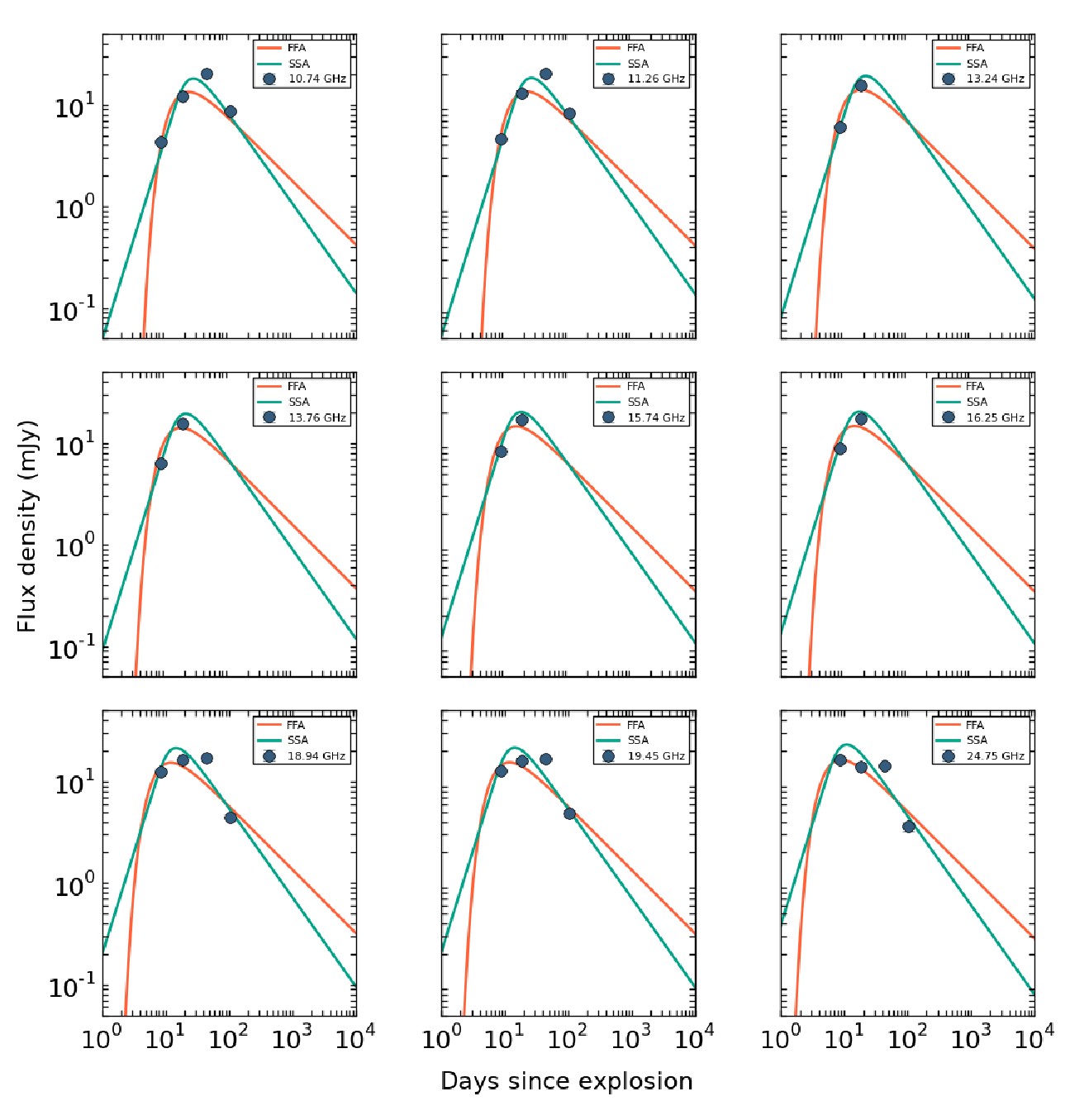
We carry out a two-variable fit to the complete radio data with FFA and SSA models. The free parameters in the FFA model are , , , and and in the SSA model are , , , and . We have a total of 112 flux density measurements at multiple epochs and frequencies. With 5 free parameters, the fit has 107 degrees of freedom. We use the chi-square minimization algorithm available in python-scipy (Virtanen, et al. 2019). In the fitting routine, 10% of flux density is added in quadrature to the JMFIT errors as systematic uncertainty to account for the calibration errors. The maximum calibration errors in various frequency bands of the VLA is % (Weiler et al. 1986). The calibration error at multiple bands of GMRT is 10% (Chandra & Kanekar 2017).
5 Results
The best-fit parameters and the reduced-chi square values are presented in Table 4. The best fit modeled light curves and spectra along with the observed data are shown in Fig. 3, 4 and 5. The reduced chi-square value becomes higher for both FFA ( = 62.0) and SSA ( = 19.2) models if the fitting routine takes only 3% of systematic error instead if 10%. However, the best fit parameters are roughly same (within 20%). From the reduced chi-square values and the fitted lightcurves and spectra, it is evident that the SSA model fits the data better than FFA. This is expected for SNe Ic since the plausible WR progenitors have fast stellar winds (few 1000 km s-1) creating a less dense CSM.
While overall data are better represented by a SSA model, it is still not a very good fit. There are a few deviations from the best fit model. In the light curve at 10.74, 11.26, 18.94, 19.45 and 24.75 GHz, the flux density measurement at 43.6 days post-explosion is slightly above the model prediction. The trend is more evident in the spectral fit (see Fig 5) where all flux density points above 10 GHz is slightly above the model prediction. We discuss this behavior in terms of a possible density enhancement in the CSM in §5.4.
| FFA | SSA |
|---|---|
| = 41.89 6.38 | = 0.72 0.03 |
| = 7.41 0.65 | = 134.55 18.88 |
| = 0.47 0.07 | = 1.99 0.02 |
| = 0.58 0.05 | = 0.85 0.04 |
| = 1.80 0.04 | = 2.40 0.10 |
| = 9.83 | = 3.63 |
| d.o.f = 107 | d.o.f = 107 |
and are the normalization parameters of flux density and optical depth, respectively. In the FFA model, and denotes the spectral and temporal evolution of the radio flux density. In the SSA model, and denotes the temporal index of flux density in the optically thick and thin regime respectively. denotes the electron energy index.


5.1 Blast-wave parameters
We model the single epoch spectra with the standard SSA model to derive the blast wave radius and post-shock magnetic field at multiple epochs (Chevalier 1998).
For a power law electron distribution of the form , the self absorbed synchrotron flux density is,
| (5) |
| (6) |
Where is the radius of the blast wave, is the distance to the SN from the observer, is the magnetic field strength and is the volume filling factor of the radio emitting region. SSA defines a spectral break frequency () below which the spectral evolution of the flux density is and above the spectral evolution is . At = the two power laws (equation 5 and 6) intersect and the corresponding flux density is . At this point equation, 5 and 6 can be inverted to obtain and assuming energy equipartition between the magnetic fields and relativistic particles. and for an electron power–law index is given by Chevalier 1998; Chevalier, & Fransson 2017 as.
| (7) |
| (8) |
In the above equations, denotes the ratio of particle energy density to magnetic field energy density. Assuming energy equipartition between relativistic particles and magnetic fields, we take =1. The constants and are tabulated as a function of in Pacholczyk 1970. in CGS units (Chevalier, & Fransson 2017). denotes the electron rest mass energy, i.e. 0.51 MeV.
The spectra of ASASSN-16fp at multiple epochs are well represented by SSA spectrum as shown in Fig. 6 with . The nearest value for which and are tabulated in Pacholczyk 1970 is for . Hence we use and corresponding and values in eqns 7 and 8. At later epochs, the spectrum peaks at lower frequencies due to the expansion of the blast wave. We find 20.49, 12.26, 07.66, 02.74 and 1.19 GHz and 13.51, 15.37, 20.00, 14.39 and 12.20 mJy on day 8, 18, 43, 104 and 272 respectively. In addition to these five epoch spectra, we also have low frequency GMRT light curves (Fig 1). The 1.39 and 0.61 GHz GMRT light curve peaks at 330.11 and 745.01 days post explosion respectively. The corresponding peak flux densities are 12.18 and 9.12 mJy at 330.11 and 745.01 days post explosion respectively. We use and at these seven epochs to derive the blast wave radius and magnetic field strength. We also find the temporal evolution of these parameters by fitting a power-law to multi-epoch values of and independently. The SSA frequency cascades as , consistent with radio SNe with dominant SSA (Soderberg et al. 2006a; Chevalier 1998). We also calculate the mean velocity of the radio emitting shell at each epoch as . The results are presented in Table 5 and Fig 7.
The radius of the shock wave is = (0.34 0.04) 1016 cm at 8.54 days post explosion and expands to = (9.56 1.45) 1016 cm at 745.01 days post explosion. The temporal evolution of shock radius can be described as 1015(t/8.54 days)0.77±0.03 cm, indicative of a decelerating blast wave. The radial evolution of shock radius is slower compared to other type Ibc SNe like SN 2003L (Soderberg et al. 2005, ;), SN 1983N (Chevalier 1998, ;) and SN 2007gr (Soderberg et al. 2010a, ;). However the temporal index is within the expected range of values i.e 0.67 1.0 (Chevalier 1996; Chevalier 1998). The post shock magnetic field evolves as )-0.83±0.04 with a radial dependence of G. The radial index of magnetic field is similar to that of other type Ic events like SN 2003L (Soderberg et al. 2005, ;) and SN 2002ap (Berger et al. 2002, ) The temporal index () of magnetic field depends on the shock radius and CSM density as = )/2]1. Thus the derived and imply the CSM density index to be . This implies that the CSM density of ASASSN-16fp is slightly flatter than the density field created by a steady stellar wind (). The derived values of and implies the ejecta density index of ASASSN-16fp to be .
The mean velocity of the shocked shell is 0.15c ( 46443 km s-1) on 8 days post-explosion indicative of a sub-relativistic velocity similar to that of normal type Ibc SNe (Chevalier & Fransson 2006). If any other absorption process like FFA defines the peak of radio light curves, the actual mean velocities derived from optical measurements will be greater than the values derived from SSA model (Chevalier 1998). The optical line velocities of ASASSN-16fp derived from absorption features at roughly the same epoch is 35000 10000 km s-1 (Prentice et al. 2018), which is less than the SSA derived value. Thus FFA is not likely to be the dominant absorption process in ASASSN-16fp.
| Days | Blastwave radius | Magnetic field | Velocity | Mass-loss rate |
|---|---|---|---|---|
| - | ( cm) | ( 10-1 Gauss) | ( c) | (10-5 ) |
| 8.54 | 0.34 0.04 | 18.27 1.02 | 0.15 0.02 | 0.44 0.16 |
| 18.56 | 0.61 0.07 | 10.78 0.40 | 0.13 0.02 | 0.71 0.23 |
| 43.60 | 1.10 0.12 | 6.54 0.21 | 0.10 0.01 | 1.45 0.46 |
| 104.25 | 2.64 0.30 | 2.43 0.11 | 0.10 0.01 | 1.14 0.38 |
| 272.00 | 5.62 0.63 | 1.07 0.04 | 0.08 0.01 | 1.52 0.50 |
| 330.11 | 4.81 0.79 | 1.25 0.01 | 0.06 0.01 | 3.06 1.56 |
| 745.01 | 09.56 1.45 | 0.57 0.01 | 0.05 0.01 | 3.20 1.52 |
The blast wave radius (R), magnetic field strength (B), mean shell velocity and mass-loss rates at seven epochs, day 8.54, 18.56, 43.60, 104.25, 272.00, 330.11 and 745.01 post explosion. We assume the date of explosion as 2016 May 25.9 (UT).


5.2 Internal energy of the radio emitting material
The minimum total internal energy of the ejecta to power the observed radio emission can be found from magnetic energy density (Soderberg et al. 2010a).
| (9) |
Assuming equipartition of energy between relativistic electrons and magnetic fields, we take = = 0.33. This places a lower limit to the total internal energy of radio emitting medium (Soderberg et al. 2010a).
| (10) |
For the derived parameters of and , we calculate = [0.370.15, 0.730.25, 1.600.53, 3.011.07, 5.691.97, 4.862.60, 7.843.91] erg on day 8.54, 18.56, 43.60, 104.25, 272.00, 330.11 and 745.01 post explosion respectively (see Table 5), comparable to other type Ibc SNe (Margutti et al. 2014). The temporal evolution of the energy can be described as 0.37 (t/8.54 days)0.65 erg (see Fig 7), obtained from the temporal indices of and . Any additional absorption process like FFA or non-equipartition values of and will further increase the energy of the radio emitting material (Chevalier & Fransson 2006; Fransson, & Björnsson 1998).
| SN | Distance | B | E | mb | References | ||||||
|---|---|---|---|---|---|---|---|---|---|---|---|
| - | (Mpc) | (days) | (GHz) | (mJy) | (erg s-1 Hz-1) | (G) | (erg s-1) | () | - | (c) | - |
| SN 2002ap | 7.3 | 7 | 1.4 | 0.3 | 3.01025 | 0.26 | 1.51045 | 0.5 | 0.90 | 0.35 | 1,2,3 |
| SN 2009bb | 40.0 | 20 | 6.0 | 19.0 | 1.91027 | 0.45 | 1.31049 | 2.0 | 0.94 | 0.85 | 4,5,6 |
| SN 2012ap | 40.0 | 18 | 8.9 | 5.7 | 8.01027 | 1.08 | 1.61049 | 3.5 | 0.74 | 0.30 | 7,8,9,10 |
| PTF11qcj | 124.0 | 10 | 1.0 | 0.7 | 1.01029 | 6.70 | 9.31048 | 120.0 | 0.80 | 0.42 | 11,12,13 |
| PTF14dby | 337.0 | 10 | 24.0 | 0.2 | 2.61028 | 1.60 | 8.01047 | 5.0 | 0.78 | 0.38 | 14,15,16 |
| ASASSN-16fpc | 17.2 | 18 | 12.3 | 15.4 | 5.21027 | 1.08 | 0.71047 | 7.1 | 0.77 | 0.13 | 17,18,19 |
| SN 1998bw | 38.0 | 16 | 6.0 | 40.0 | 8.01028 | 0.40 | 1.01049 | 0.25 | 0.77 | 1.30 | 20,21,22 |
References: (1) Berger et al. 2002, (2) Smartt et al. 2002, (3) Gal-Yam et al. 2002, (4) Soderberg et al. 2010b, (5) Pignata et al. 2009, (6) Pignata et al. 2011, (7) Chakraborti et al. 2015, (8) Margutti et al. 2014, (9) Springob et al. 2007, (10) Milisavljevic et al. 2012, (11) Corsi et al. 2014, (12) Bloom et al. 2012, (13) Palliyaguru et al. 2019, (14) Yaron, & Gal-Yam 2012, (15) Laher et al. 2014, (16) Corsi et al. 2016, (17) Yamanaka et al. 2017, (18) Holoien et al. 2016, (19) Elias-Rosa et al. 2016, (20) Kulkarni et al. 1998, (21) Li, & Chevalier 1999, (22) Galama et al. 1998.
Note - Radio luminosity () is peak spectral luminosity at 5 GHz. The time to reach for SN 2002ap, SN 2009bb, SN 2012ap, PTF11qcj, PTF14dby, ASASSN-16fp and SN 1998bw are 3, 52, 38, 100, 47, 104 and 12 days post explosion respectively.
Note - The parameters , , and are derived at the time of SSA peak assuming equipartition of energy between relativistic electrons and magnetic field.
, and denotes the peak frequency, peak flux density and time to peak respectively of the SSA modelled spectra (Chevalier 1998).
denotes the shock deceleration parameter.
The parameters of ASASSN-16fp are from this work.
5.3 Mass loss rate of the progenitor star
The mass-loss rate of the progenitor star can be derived from the post shock magnetic field energy density (Chevalier 1998; Soderberg et al. 2006a).
| (11) |
where is the velocity of the stellar wind of the progenitor star. Assuming = 0.33 and a wind velocity of 1000 km s-1, typical of a WR star (Cappa et al. 2004), we derive the mass-loss rate to be, 10-5 on day 8.54 post explosion. The mass-loss rate is 10-5 on day 745 post explosion (see Table 5). The mass-loss rates at multiple epochs suggest that the progenitor of ASASSN-16fp has gone through variable mass-loss rates in the years prior explosion. The mass-loss rate at 37 years prior explosion is 7.3 times greater than the mass-loss rate at 1 year prior explosion for a stellar wind velocity of 1000 km s-1. The derived mass-loss rates are consistent with the mass-loss rate seen in Galactic WR stars () (Abbott et al. 1986; Leitherer et al. 1995; Leitherer et al. 1997; Chapman et al. 1999; Cappa et al. 2004).
The equipartition assumption puts a lower limit on the mass-loss rate. In a realistic scenario, the SN post shock energy is distributed among electrons, protons/ions and magnetic fields and the values of and are likely less than 0.33 (Chevalier & Fransson 2006). For more realistic values, and (Terreran et al. 2019), we derive the mass-loss rates to be () at various epochs spanning days post-explosion. This is consistent with the mass-loss rate estimate of ASASSN-16fp () from X-ray observations (Terreran et al. 2019).
5.4 Density structure of CSM
Radio light curves trace the density structure of the CSM. The density of the CSM need not be uniform due to variable mass-loss rate, variable wind velocity of the progenitor star, ejected stellar envelopes of progenitors, etc. The non-uniform density structure of the CSM can cause jumps in the radio light curve (Soderberg et al. 2006a). In the radio light curve of ASASSN-16fp, we see flux density enhancements on day 43.6 post-explosion at frequencies above 10 GHz where the emission is optically thin. The effect is also seen in the spectra (see Fig. 5) where all the optically thin flux density measurements are above the model prediction. We interpret this as a signature of non-uniform CSM density at a radius of 1.10 1016 cm. The flux density scales as , for SSA dominated radio emission (Chevalier 1998). Assuming constant through out the evolution, and the radio flux density . For , . The flux density enhancement seen on day 43 from ASASSN-16fp is 1.5 times that of the standard model prediction. Thus the density enhancement in CSM is only 1.2. This could be due to small scale clumping within the stellar wind (Moffat 2008; Smith 2014). The CSM of WR stars are known to be significantly disturbed and there are X-ray observations that show evidence for dense clumps (Hillier 2003). Assuming a stellar wind velocity of 1000 km s-1, typical of WR stars (Cappa et al. 2004), the density enhancement could be due to a mass-loss event happened 3.5 years prior explosion. These sorts of small scale flux density enhancements are seen in 50% of SNe Ib/c (Soderberg et al. 2006a).
6 A comparison with other SNe Ic-BL
In this section, we compare the properties of ASASSN-16fp with other radio bright SNe Ic-BL with out GRB association. The properties of a few SNe Ic-BL from radio modeling are compiled in Table 6. We also include the first prototypical GRB associated SN 1998bw/GRB980425 in the table for comparison. The 5 GHz light curve of ASASSN-16fp peaks at 104 days post-explosion with spectral luminosity 5.21027 placing it as one of the luminous radio SNe with luminosities similar to SN 2009bb (Soderberg et al. 2010b) and SN 2012ap (Chakraborti et al. 2015). The peak radio spectral luminosity of ASASSN-16fp is within the broad distribution of radio luminosities of SNe Ibc (Soderberg et al. 2006b) attributed to the range of CSM densities observed in Galactic WR stars (Chevalier & Fransson 2006). Besides, the variation in the parameters and may also contribute to the large range of radio luminosity (Chevalier & Fransson 2006). The light curve of ASASSN-16fp evolves slightly slower compared to the typical rise time of 5 GHz light curve (10-30 days) of SNe Ib/c (Weiler et al. 1998). The 5 GHz spectral luminosity of ASASSN-16fp is 20 times smaller than the spectral luminosity of PTF11qcj (Corsi et al. 2014; Corsi et al. 2016) that peaks at a similar time (100 days post-explosion). The mass-loss rate of PTF11qcj is 17 times more than that of ASASSN-16fp owing to the brighter radio emission possibly due to denser CSM. The mean shock velocity of ASASSN-16fp on 18 days post-explosion is 0.13c consistent with the mean shock velocities of normal SNe Ib/c (Soderberg et al. 2006b, 0.1-0.15c;). Chevalier 1998 compiled mean shock velocities of a sample of SNe Ib/c and the mean shock velocity of ASASSN-16fp closely resemble the shock velocity of SN 1993N at similar epoch. A comparison with the mean shock velocities of SNe Ic-BL suggests that ASASSN-16fp has the slowest shock with velocity at least a factor of 2 less than the rest of the SNe Ic-BL in the Table 6. The shock velocity of ASASSN-16fp is 10 times slower compared to GRB associated SN 1998bw (Kulkarni et al. 1998). Thus ASASSN-16fp further emphasizes that broad lines in the optical spectra cannot be considered as the proxy for relativistic ejecta as also seen in SN 2002ap (Berger et al. 2003). The difference in shock velocity could be either due to the difference in CSM density or due to the SN property itself like initial explosion energy or ejecta mass. The different SNe Ic-BL are characterized by roughly similar shock deceleration parameter (). The shock deceleration parameter of ASASSN-16fp is , indicative of WR like radiative progenitor star similar to PTF11qcj (Corsi et al. 2014) and PTF11dby (Corsi et al. 2016; Horesh et al. 2013). The magnetic field of ASASSN-16fp at 18 days post-explosion (1.1 G) is higher than the magnetic fields seen in normal SNe Ib/c (Chevalier 1998, 0.2-0.6 G;) and is similar to the magnetic field of SN 2012ap (Chakraborti et al. 2015). The mass-loss rates of the progenitors of SNe Ic-BL are in the range of (0.3-5)10-6 yr-1 except for PTF11qcj (Corsi et al. 2014). The relatively lower mass-loss rates are indicative of compact progenitors of these SNe driving faster stellar winds. The internal energy of the radio-emitting material of ASASSN-16fp is 46 times greater than SN 2002ap (Berger et al. 2003) and 100 times smaller than SN 1998bw (Kulkarni et al. 1998), placing it in a phase space between SN 2002ap and SN 1998bw in terms of energetics. The radio light curve of ASASSN-16fp shows remarkable similarity with the radio light curves of PTF11qcj (Corsi et al. 2014) showing achromatic short time scale variability (Corsi et al. 2014, see Fig 11 and 12 of). PTF11qcj exhibits a factor of 2 enhancement in flux density at radius 1.71017 cm owing to small-scale density fluctuations in the CSM. ASASSN-16fp also shows small scale flux density enhancement at radius =1.11016 cm (see §5.4).
7 Summary
We present extensive radio observations of a Type Ic supernova, ASASSN-16fp spanning a frequency range of GHz and a temporal range of days post-explosion. We model the radio data with the standard model and our main results are the following
- 1.
The observations are best represented by a model in which the dominant absorption process is SSA during the time-scale probed by the radio data.
- 2.
Assuming equipartition of energy between relativistic particles and magnetic fields ( and ), we estimate the shock radius and velocity to be cm and c respectively at 8 days post-explosion. The shock velocity is sub-relativistic as seen in normal type Ic SNe implying that the broad absorption lines in the optical spectra do not indicate relativistic ejecta.
- 3.
The evolution of the shock radius and magnetic field can be represented as t0.77±0.03 and t-0.83±0.04 respectively, implying a CSM density profile and an outer ejecta density profile .
- 4.
We infer the temporal evolution of the total internal energy of the radio-emitting material to be 0.37 (t/8.54 days)0.65 erg, consistent with the normal type Ibc SN population.
- 5.
We determine the mass-loss rate of the progenitor star to be from equipartition values, consistent with the mass-loss rate of Galactic WR stars.
- 6.
The radio light curves and spectra show the signature of density enhancement in the CSM at a radius of cm from the explosion center possibly due to a small scale clumping in the stellar wind 3.5 years prior explosion.
- 7.
A comparison of ASASSN-16fp parameters with other SNe Ic-BL suggests that ASASSN-16fp is fairly radio luminous similar to SN 2012ap and SN 2009bb with slower shock typical of normal SNe Ibc.
Acknowledgements
P.C. acknowledges support from the Department of Science and Technology via SwaranaJayanti Fellowship award (file no.DST/SJF/PSA-01/2014-15). We thank the staff of the GMRT that made these observations possible. GMRT is run by the National Centre for Radio Astrophysics of the Tata Institute of Fundamental Research. The National Radio Astronomy Observatory is a facility of the National Science Foundation operated under cooperative agreement by Associated Universities, Inc.
References
- Abbott et al. (1986) Abbott, D. C., Beiging, J. H., Churchwell, E., & Torres, A. V. 1986, ApJ, 303, 239
- Alexander et al. (2016) Alexander, K. D., Laskar, T., & Berger, E. 2016, GRB Coordinates Network, Circular Service, No. 20313, #1 (2016), 20313, 1
- Argo et al. (2016) Argo, M. K., Romero-Canizales, C., Beswick, R., & Prieto, J. L. 2016, The Astronomer’s Telegram, 9147,
- Ashall et al. (2017) Ashall, C., Pian, E., Mazzali, P. A., et al. 2017, arXiv:1702.04339
- Berger et al. (2002) Berger, E., Kulkarni, S. R., & Chevalier, R. A. 2002, ApJ, 577, L5
- Berger et al. (2003) Berger, E., Kulkarni, S. R., Pooley, G., et al. 2003, Nature, 426, 154
- Bersten et al. (2014) Bersten, M. C., Benvenuto, O. G., Folatelli, G., et al. 2014, AJ, 148, 68
- Bloom et al. (2012) Bloom, J. S., Richards, J. W., Nugent, P. E., et al. 2012, PASP, 124, 1175
- Burrows, et al. (2005) Burrows D. N., et al., 2005, SSRv, 120, 165
- Cano et al. (2017) Cano, Z., Izzo, L., de Ugarte Postigo, A., et al. 2017, A&A, 605, A107
- Cao et al. (2013) Cao, Y., Kasliwal, M. M., Arcavi, I., et al. 2013, ApJ, 775, L7
- Cappa et al. (2004) Cappa, C., Goss, W. M., & van der Hucht, K. A. 2004, AJ, 127, 2885
- Chakraborti et al. (2015) Chakraborti, S., Soderberg, A., Chomiuk, L., et al. 2015, ApJ, 805, 187
- Chandra & Kanekar (2017) Chandra P., Kanekar N., 2017, ApJ, 846, 111
- Chapman et al. (1999) Chapman, J. M., Leitherer, C., Koribalski, B., Bouter, R., & Storey, M. 1999, ApJ, 518, 890
- Chevalier (1982a) Chevalier, R. A. 1982a, ApJ, 258, 790
- Chevalier (1982b) Chevalier, R. A. 1982b, ApJ, 259, 302
- Chevalier (1996) Chevalier, R. A. 1996, Radio Emission from the Stars and the Sun, 125
- Chevalier (1998) Chevalier, R. A. 1998, ApJ, 499, 810
- Chevalier & Fransson (2006) Chevalier, R. A., & Fransson, C. 2006, ApJ, 651, 381
- Chevalier, & Fransson (2017) Chevalier, R. A., & Fransson, C. 2017, Handbook of Supernovae, 875
- Chu (2002) Chu, Y.-H. 2002, Interacting Winds from Massive Stars, 260, 109
- Clocchiatti et al. (1996) Clocchiatti, A., Wheeler, J. C., Brotherton, M. S., et al. 1996, ApJ, 462, 462
- Corsi et al. (2014) Corsi, A., Ofek, E. O., Gal-Yam, A., et al. 2014, ApJ, 782, 42
- Corsi et al. (2016) Corsi, A., Gal-Yam, A., Kulkarni, S. R., et al. 2016, ApJ, 830, 42
- D’Ai et al. (2016) D’Ai, A., Kennea, J. A., Krimm, H. A., et al. 2016, GRB Coordinates Network, Circular Service, No. 20296, #1 (2016), 20296, 1
- de Ugarte Postigo et al. (2016) de Ugarte Postigo, A., Cano, Z., Izzo, L., et al. 2016, GRB Coordinates Network, Circular Service, No. 20342, #1 (2016), 20342, 1
- Dessart et al. (2012) Dessart, L., Hillier, D. J., Li, C., & Woosley, S. 2012, MNRAS, 424, 2139
- Ensman, & Woosley (1988) Ensman, L. M., & Woosley, S. E. 1988, ApJ, 333, 754
- Eldridge et al. (2015) Eldridge, J. J., Fraser, M., Maund, J. R., & Smartt, S. J. 2015, MNRAS, 446, 2689
- Elias-Rosa et al. (2016) Elias-Rosa, N., Mattila, S., Lundqvist, P., et al. 2016, The Astronomer’s Telegram, 9090,
- Filippenko (1997) Filippenko, A. V. 1997, ARA&A, 35, 309
- Foley et al. (2003) Foley, R. J., Papenkova, M. S., Swift, B. J., et al. 2003, PASP, 115, 1220
- Frail et al. (2005) Frail, D. A., Soderberg, A. M., Kulkarni, S. R., et al. 2005, ApJ, 619, 994
- Fransson, & Björnsson (1998) Fransson, C., & Björnsson, C.-I. 1998, ApJ, 509, 861
- Fransson et al. (1996) Fransson, C., Lundqvist, P., & Chevalier, R. A. 1996, ApJ, 461, 993
- Frey et al. (2013) Frey, L. H., Fryer, C. L., & Young, P. A. 2013, ApJ, 773, L7
- Galama et al. (1998) Galama, T. J., Vreeswijk, P. M., van Paradijs, J., et al. 1998, Nature, 395, 670
- Gal-Yam et al. (2002) Gal-Yam, A., Ofek, E. O., & Shemmer, O. 2002, MNRAS, 332, L73
- Greisen (2003) Greisen E. W., 2003, ASSL, 109, ASSL..285
- Groh et al. (2013) Groh, J. H., Georgy, C., & Ekström, S. 2013, A&A, 558, L1
- Grupe et al. (2016) Grupe, D., Brown, P., Dong, S., et al. 2016, The Astronomer’s Telegram, 9088,
- Hachinger et al. (2012) Hachinger, S., Mazzali, P. A., Taubenberger, S., et al. 2012, MNRAS, 422, 70
- Hillier (2003) Hillier, D. J. 2003, A Massive Star Odyssey: From Main Sequence to Supernova, 70
- Hjorth et al. (2003) Hjorth, J., Sollerman, J., Møller, P., et al. 2003, Nature, 423, 847
- Holoien et al. (2016) Holoien, T. W.-S., Stanek, K. Z., Brown, J. S., et al. 2016, The Astronomer’s Telegram, 9086,
- Horesh et al. (2013) Horesh, A., Stockdale, C., Fox, D. B., et al. 2013, MNRAS, 436, 1258
- Kumar et al. (2018) Kumar, B., Singh, A., Srivastav, S., Sahu, D. K., & Anupama, G. C. 2018, MNRAS, 473, 3776
- Kulkarni et al. (1998) Kulkarni, S. R., Frail, D. A., Wieringa, M. H., et al. 1998, Nature, 395, 663
- Laher et al. (2014) Laher, R. R., Surace, J., Grillmair, C. J., et al. 2014, PASP, 126, 674
- Leitherer et al. (1995) Leitherer, C., Chapman, J. M., & Koribalski, B. 1995, ApJ, 450, 289
- Leitherer et al. (1997) Leitherer, C., Chapman, J. M., & Koribalski, B. 1997, ApJ, 481, 898
- Li, & Chevalier (1999) Li, Z.-Y., & Chevalier, R. A. 1999, ApJ, 526, 716
- Mazzali et al. (2003) Mazzali, P. A., Deng, J., Tominaga, N., et al. 2003, ApJ, 599, L95
- Mazzali et al. (2006) Mazzali, P. A., Deng, J., Nomoto, K., et al. 2006, Nature, 442, 1018
- Maeda (2013) Maeda, K. 2013, ApJ, 762, 14
- Margutti et al. (2014) Margutti, R., Milisavljevic, D., Soderberg, A. M., et al. 2014, ApJ, 797, 107
- McMullin, et al. (2007) McMullin J. P., Waters B., Schiebel D., Young W., Golap K., 2007, ASPC, 127, ASPC..376
- Milisavljevic et al. (2012) Milisavljevic, D., Fesen, R., Soderberg, A., et al. 2012, Central Bureau Electronic Telegrams 3037, 2
- Milisavljevic et al. (2015) Milisavljevic, D., Margutti, R., Parrent, J. T., et al. 2015, ApJ, 799, 51
- Modjaz et al. (2016) Modjaz, M., Liu, Y. Q., Bianco, F. B., & Graur, O. 2016, ApJ, 832, 108
- Mooley et al. (2016) Mooley, K. P., Fender, R. P., Cantwell, T., et al. 2016, The Astronomer’s Telegram, 9134,
- Moffat (2008) Moffat, A. F. J. 2008, Clumping in Hot-Star Winds, 17
- Nayana & Chandra (2016) Nayana, A. J., & Chandra, P. 2016, The Astronomer’s Telegram, 9201,
- Nayana & Chandra (2016) Nayana, A. J., & Chandra, P. 2016, GRB Coordinates Network, Circular Service, No. 20344, #1 (2016), 20344, 1
- Nayana A. et al. (2018) Nayana A., J., Chandra, P., & Ray, A. K. 2018, ApJ, 863, 163
- Nugis & Lamers (2000) Nugis, T., & Lamers, H. J. G. L. M. 2000, A&A, 360, 227
- Pacholczyk (1970) Pacholczyk, A. G. 1970, Series of Books in Astronomy and Astrophysics
- Palliyaguru et al. (2019) Palliyaguru, N. T., Corsi, A., Frail, D. A., et al. 2019, ApJ, 872, 201
- Pian et al. (2000) Pian, E., Amati, L., Antonelli, L. A., et al. 2000, ApJ, 536, 778
- Pignata et al. (2009) Pignata, G., Maza, J., Hamuy, M., et al. 2009, Central Bureau Electronic Telegrams 1731, 1
- Pignata et al. (2011) Pignata, G., Stritzinger, M., Soderberg, A., et al. 2011, ApJ, 728, 14
- Podsiadlowski (1992) Podsiadlowski, P. 1992, PASP, 104, 717
- Prasad & Chengalur (2012) Prasad, J., & Chengalur, J. 2012, Experimental Astronomy, 33, 157
- Prentice et al. (2018) Prentice, S. J., Ashall, C., Mazzali, P. A., et al. 2018, MNRAS, 478, 4162
- Smartt et al. (2002) Smartt, S. J., Vreeswijk, P. M., Ramirez-Ruiz, E., et al. 2002, ApJ, 572, L147
- Sahu et al. (2008) Sahu, D. K., Tanaka, M., Anupama, G. C., et al. 2008, ApJ, 680, 580
- Smartt (2009) Smartt, S. J. 2009, ARA&A, 47, 63
- Smith et al. (2011) Smith, N., Li, W., Filippenko, A. V., & Chornock, R. 2011, MNRAS, 412, 1522
- Smith (2014) Smith, N. 2014, ARA&A, 52, 487
- Soderberg et al. (2005) Soderberg, A. M., Kulkarni, S. R., Berger, E., et al. 2005, ApJ, 621, 908
- Soderberg et al. (2006a) Soderberg, A. M., Chevalier, R. A., Kulkarni, S. R., & Frail, D. A. 2006a, ApJ, 651, 1005
- Soderberg et al. (2006b) Soderberg, A. M., Nakar, E., Berger, E., et al. 2006b, ApJ, 638, 930
- Soderberg et al. (2010a) Soderberg, A. M., Brunthaler, A., Nakar, E., Chevalier, R. A., & Bietenholz, M. F. 2010a, ApJ, 725, 922
- Soderberg et al. (2010b) Soderberg, A. M., Chakraborti, S., Pignata, G., et al. 2010b, Nature, 463, 513
- Springob et al. (2007) Springob, C. M., Masters, K. L., Haynes, M. P., et al. 2007, ApJS, 172, 599
- Sutaria et al. (2003) Sutaria, F. K., Chandra, P., Bhatnagar, S., & Ray, A. 2003, A&A, 397, 1011
- Swarup, et al. (1991) Swarup G., Ananthakrishnan S., Kapahi V. K., Rao A. P., Subrahmanya C. R., Kulkarni V. K., 1991, CuSc, 60, 95
- Tanaka et al. (2009) Tanaka, M., Tominaga, N., Nomoto, K., et al. 2009, ApJ, 692, 1131
- Taubenberger et al. (2006) Taubenberger, S., Pastorello, A., Mazzali, P. A., et al. 2006, MNRAS, 371, 1459
- Terreran et al. (2019) Terreran, G., Margutti, R., Bersier, D., et al. 2019, ApJ, 883, 147
- Valenti et al. (2008) Valenti, S., Benetti, S., Cappellaro, E., et al. 2008, MNRAS, 383, 1485
- Virtanen, et al. (2019) Virtanen P., et al., 2019, arXiv, arXiv:1907.10121
- Weiler et al. (1986) Weiler, K. W., Sramek, R. A., Panagia, N., van der Hulst, J. M., & Salvati, M. 1986, ApJ, 301, 790
- Weiler et al. (1998) Weiler, K. W., Van Dyk, S. D., Montes, M. J., et al. 1998, ApJ, 500, 51
- Weiler et al. (2002) Weiler, K. W., Panagia, N., Montes, M. J., & Sramek, R. A. 2002, ARA&A, 40, 387
- Woosley et al. (1995) Woosley, S. E., Langer, N., & Weaver, T. A. 1995, ApJ, 448, 315
- Yamanaka et al. (2017) Yamanaka, M., Nakaoka, T., Tanaka, M., et al. 2017, ApJ, 837, 1
- Yaron, & Gal-Yam (2012) Yaron, O., & Gal-Yam, A. 2012, PASP, 124, 668
- Yoon et al. (2010) Yoon, S.-C., Woosley, S. E., & Langer, N. 2010, ApJ, 725, 940
- Yoon (2015) Yoon, S.-C. 2015, Publ. Astron. Soc. Australia, 32, e015
- Zwart, et al. (2008) Zwart J. T. L., et al., 2008, MNRAS, 391, 1545