跳到论文正文
W Papers独立论文阅读器 arXiv:2003.02681 论文正文 计算阅读时间 · 0%
引用这篇论文根据当前论文元数据生成,正式投稿前建议核对。


License: arXiv.org perpetual non-exclusive license
arXiv:2003.02681v1 [cs.LG] 05 Mar 2020
 

Stochastic Linear Contextual Bandits with Diverse Contexts


Weiqiang Wu          Jing Yang          Cong Shen

London Stock Exchange          The Pennsylvania State University          University of Virginia

Abstract

In this paper, we investigate the impact of context diversity on stochastic linear contextual bandits. As opposed to the previous view that contexts lead to more difficult bandit learning, we show that when the contexts are sufficiently diverse, the learner is able to utilize the information obtained during exploitation to shorten the exploration process, thus achieving reduced regret. We design the LinUCB-d algorithm, and propose a novel approach to analyze its regret performance. The main theoretical result is that under the diverse context assumption, the cumulative expected regret of LinUCB-d is bounded by a constant. As a by-product, our results improve the previous understanding of LinUCB and strengthen its performance guarantee.

1 Introduction

In many applications, such as resource allocation in cloud computing platforms, or treatment selection for patients in clinical trials, the diverse user preferences and characteristics impose urgent need of personalized decision-making. In order to make optimal decisions for different individuals, the decision maker must learn a model to predict the reward when a decision is taken under different contexts. This problem is often formulated as a contextual bandit problem (Auer, 2003; Langford and Zhang, 2008), which generalizes the classical multi-armed bandit (MAB) framework (Lai and Robbins, 1985; Auer et al., 2002; Bubeck and Cesa-Bianchi, 2012; Agrawal and Goyal, 2012; Agrawal and Goyal, 2013).

The inclusion of contextual information in the decision-making process introduces more uncertainty into the MAB framework and creates significant challenges for the learning problem. Part of the difficulty in contextual MAB comes from the increased problem dimension, as context is added as part of the unknown environment. Existing literature mostly focuses on developing bandit algorithms and providing theoretical analysis by treating the context as structureless side information. The resulting models and algorithms are generic, but represent a “worst case” scenario since very little, if any, structure of the context is exploited.

In many real-world applications, however, context often exhibits sufficient level of diversity, which has been largely overlooked in the existing studies. For example, user profile is considered as the context in recommendation systems (Li et al., 2010). When the system serves a large number of users, the group of user profiles is likely to be very diverse. As another example, contextual MAB has been adopted in service placement of mobile edge computing, which utilizes the time of day and mobile user types as the context (Chen and Xu, 2019).

It is not difficult to see that in these applications, the context arrival exhibits sufficient diversity that may be beneficial to the bandit algorithm design. Intuitively, the diverse contexts create opportunities for the learner to reduce the learning regret: when an arm is pulled frequently as the optimal arm for certain contexts, its parameters can be estimated accurately with the rewards obtained during exploitation. Therefore, the learner does not have to spend much time exploring it when the instantaneous context is not in favor for it, thus shortening the exploration stage and speeding up the convergence.

In this paper, we demonstrate this optimistic view of context diversity by investigating the impact of diverse contextual information on the learning regret under the stochastic linear contextual bandits framework (Bastani et al., 2017). We show that, instead of considering the context as part of the “uncontrollable” environment and passively “reacting” to the incoming context, proactively interacting between context and arm exploration allows learning to transfer between different contexts and leads to much better overall performance. Specifically, we consider a set of KK arms, where the parameter of each arm is represented by a dd-dimensional vector unknown to the learner. When an arm aa is pulled under a context cc, the obtained reward is the inner product of the parameter of the arm and a feature vector determined by arm aa and context cc, corrupted by noise. The objective of the learner is to use the information contained in the observed rewards to decide an arm to pull in response to the instantaneous context. Assuming independent and identically distributed (i.i.d.) contexts, we aim to show that when the contexts are sufficiently diverse, the cumulative learning regret in expectation can be bounded by a constant.

The main contributions of this paper are three-fold. First, we formally introduce the concept of context diversity into the stochastic linear contextual bandit framework and present a novel geometric interpretation. Such geometric interpretation provides an intuitive viewpoint to understand and analyze the impact of context diversity on the learning performance of stochastic linear contextual bandits.

Second, we propose an Upper Confidence Bound (UCB) type algorithm, termed as LinUCB-d, for the contextual bandit model. The new formulation of LinUCB-d enables a unique approach to characterize the impact of context diversity and achieve finite cumulative regret. The results also extend the existing understanding of LinUCB and strengthen its performance guarantee.

Third, we design a novel approach to analyze the performance of LinUCB-d. There are two distinct features of our approach: First, we relate the uncertainty in the estimated rewards with the solution to a constrained optimization problem, and leverage the optimality of the estimator to bound the corresponding frequency of bad decisions during the learning process. Second, we propose a frame-based approach to isolate the error events on a frame basis and make the regret tractable. These techniques are novel and may find useful in other related settings.

2 Problem Formulation

We consider a set of KK items (arms) denoted as [K]={1,2,…,K}[K]=\{1,2,\ldots,K\}. Assume for each a∈[K]a\in[K] there is a fixed but unknown parameter vector 𝜽⁡(a)∈ℝd\bm{\theta}(a)\in{\mathbb{R}^{d}}. At each time tt, the learner observes a random context ctc_{t}, which is generated according to an unknown distribution. Next, the learner decides to pull an arm at∈[K]a_{t}\in[K] based on the information available. The incurred reward yty_{t} is given by yt=r⁡(at,ct)+ηty_{t}=r(a_{t},c_{t})+\eta_{t}, where ηt\eta_{t} is a random noise, and r⁡(at,ct)r(a_{t},c_{t}) is a linear function of 𝜽⁡(at)\bm{\theta}({a_{t}}) and the feature vector 𝐱⁡(at,ct)∈ℝd\mathbf{x}({a_{t}},{c_{t}})\in\mathbb{R}^{d}, i.e.,

r⁡(at,ct):=𝜽⊺​(at)​𝐱​(at,ct).\displaystyle r(a_{t},c_{t}):=\bm{\theta}^{\intercal}({a_{t}})\mathbf{x}({a_{t}},{c_{t}}). (1)

Here we use 𝐱⊺\mathbf{x}^{\intercal} to denote the transpose of vector 𝐱\mathbf{x}.

Let 𝒞\mathcal{C} be the set of all contexts. For any a∈[K]a\in[K], define

𝒞a\displaystyle\mathcal{C}_{a} :={c∈𝒞∣r(a,c)>r(b,c),∀b∈[K]\{a}},\displaystyle:=\left\{c\in\mathcal{C}\mid r(a,c)>r(b,c),\forall b\in[K]\backslash\{a\}\right\}, (2)
𝒳a\displaystyle\mathcal{X}_{a} :={𝐱⁡(a,c)∈ℝd∣c∈𝒞a},\displaystyle:=\left\{\mathbf{x}(a,c)\in{\mathbb{R}^{d}}\mid c\in\mathcal{C}_{a}\right\}, (3)

i.e., 𝒞a\mathcal{C}_{a} is the subset of contexts under which arm aa is the best arm rendering the maximum expected reward, and 𝒳a\mathcal{X}_{a} is the set of feature vectors when arm aa is pulled under contexts in 𝒞a\mathcal{C}_{a}. Let ℱt=σ⁡(c1,a1,y1,…,ct−1,at−1,yt−1,ct,at)\mathcal{F}_{t}=\sigma(c_{1},a_{1},y_{1},\dots,c_{t-1},a_{t-1},y_{t-1},c_{t},a_{t}) be the σ\sigma-field summarizing the information available just before yty_{t} is observed. We make the following assumptions throughout the paper.

Assumption 1
  1. 1)

    Bounded parameters: For any a∈[K]a\in[K], c∈𝒞c\in\mathcal{C}, we have ‖𝜽⁡(a)‖2≤s\|\bm{\theta}(a)\|_{2}\leq s, ‖𝐱⁡(a,c)‖2≤l\|\mathbf{x}(a,c)\|_{2}\leq l.

  2. 2)

    Minimum reward gap: For any a,b∈[K]a,b\in[K], b≠ab\neq a, c∈𝒞ac\in\mathcal{C}_{a}, r⁡(a,c)−r⁡(b,c)≥Δ>0r(a,c)-r(b,c)\geq\Delta>0.

  3. 3)

    Conditionally 1-subgaussian noise: Given ℱt\mathcal{F}_{t}, ηt\eta_{t} is conditionally 1-subgaussian with 𝔼⁡[ηt|ℱt]=0\mathbb{E}[\eta_{t}|\mathcal{F}_{t}]=0, 𝔼⁡[exp⁡(λ​ηt)|ℱt]≤exp⁡(λ22)\mathbb{E}[\exp(\lambda\eta_{t})|\mathcal{F}_{t}]\leq\exp(\frac{\lambda^{2}}{2}) for any λ>0\lambda>0.

  4. 4)

    Stochastic context arrivals: In each time tt, ctc_{t} is drawn from the context set 𝒞\mathcal{C} in an i.i.d. fashion according to a distribution ν\nu.

  5. 5)

    Diverse contexts: For any arm a∈[K]a\in[K], λmin​(𝔼c∼ν​[𝐱⁡(a,c)​𝐱​(a,c)⊺|c∈𝒞a])>0\lambda_{\min}(\mathbb{E}_{c\sim\nu}[\mathbf{x}(a,c)\mathbf{x}(a,c)^{\intercal}|c\in\mathcal{C}_{a}])>0, where λmin​(A)\lambda_{\min}(A) is the smallest eigenvalue of AA.

Assumption 1.1 ensures that the maximum regret at any step is bounded. Assumption 1.2 indicates that under a given context cc, the optimal arm is strictly better than any other sub-optimal arms. Such a reward gap affects the convergence rate of the proposed algorithm (similar to the stochastic MAB setting). Assumption 1.3 allows us to utilize the induced super-martingale to derive exponentially decaying tail bound of the estimation error. We note that all three assumptions on the bandit model are standard in the bandit literature or in the study of linear bandits.

Assumption 1.4 is a non-critical assumption made for ease of exposition. Essentially, what is required for the main results to hold is the ergodicity of the context arrival process, i.e., contexts lying in certain favorable subsets recur frequently in time.

Assumption 1.5 is however critical for our main results to hold. It is equivalent to the condition that

ℙ[λmin(Φa⊺Φa)>0]>0,∀a∈[K],\displaystyle\mathbb{P}[\lambda_{\min}(\Phi_{a}^{\intercal}\Phi_{a})>0]>0,\quad\forall a\in[K], (4)

where Φa\Phi_{a} is a random matrix whose columns are dd feature vectors associated with arm aa and dd i.i.d. contexts drawn according to the conditional distribution of cc given c∈𝒞ac\in\mathcal{C}_{a}. It implies two conditions: First, all arms in [K][K] could be optimal under certain contexts, i.e., 𝒞a≠∅\mathcal{C}_{a}\neq\emptyset. Second, for all contexts in favor of the same arm (i.e., contexts in 𝒞a\mathcal{C}_{a}), they are sufficiently diverse so that the corresponding feature vectors span ℝd\mathbb{R}^{d}. If the first condition does not hold, the arms that are strictly sub-optimal have to be explored sufficiently frequently in order to be distinguished from the optimal arms, thus an O⁡(log⁡T)O(\log T) regret is unavoidable in this situation. For the second condition, although it seems strict at first sight, it is actually quite reasonable in practice. This is because if a feature vector falls in 𝒳a\mathcal{X}_{a}, we would expect that feature vectors drawn from a small neighborhood of it fall in 𝒳a\mathcal{X}_{a} as well. Since small perturbations of a vector can form a full-rank matrix, it is thus reasonable to assume span​(𝒳a)=ℝd\mbox{span}(\mathcal{X}_{a})=\mathbb{R}^{d}.

Assume {𝐱⁡(a,c)}a,c\{\mathbf{x}(a,c)\}_{a,c} is given and {𝜽⁡(a)}a\{\bm{\theta}(a)\}_{a} is unknown a priori. The cumulative regret of an online learning algorithm is defined as

RT:=∑t=1Tr⁡(at∗,ct)−∑t=1Tyt,\displaystyle R_{T}:=\sum_{t=1}^{T}r(a_{t}^{*},c_{t})-\sum_{t=1}^{T}y_{t}, (5)

where at∗:=arg⁡maxa∈[K]⁡r⁡(a,ct)a_{t}^{*}:=\arg\max_{a\in[K]}r(a,c_{t}). While sublinear learning regret has been established for such linear contextual bandits (Abbasi-Yadkori et al., 2011; Chu et al., 2011), our objective is to investigate the fundamental impact of context diversity on the expected regret 𝔼⁡[RT]\mathbb{E}[R_{T}].

3 Algorithm

The existing linear contextual bandit algorithms such as the celebrated LinUCB (Li et al., 2010) can be directly applied to the considered bandit problem. However, such approaches ignore the diversity in context arrivals and offer little insight to the understanding of diversity. In this section, we propose a Linear Upper Confidence Bound algorithm to manifest the impact of the diversity of context on the scaling of the learning regret. To distinguish it from LinUCB, we term it LinUCB-d.

We label all contexts that have appeared in the order of their first appearances. We assume there are ntn_{t} different contexts that have appeared before time tt. With a slight abuse of notation, we denote the subset of those contexts as 𝒞t\mathcal{C}_{t}. Besides, we add dd dummy contexts, and denote the subset as 𝒞0\mathcal{C}_{0}. In the following, we use c∈{1,2,…,nt+d}c\in\{1,2,\ldots,n_{t}+d\} to index the contexts, while the first ntn_{t} contexts are in 𝒞t\mathcal{C}_{t} and the last dd are the added dummy ones. For the added dummy contexts, we assume the corresponding feature vector 𝐱⁡(a,nt+j)=l​𝐞j\mathbf{x}(a,{n_{t}+j})=l\mathbf{e}_{j}, j=1,…,dj=1,\ldots,d, where 𝐞j∈ℝd\mathbf{e}_{j}\in\mathbb{R}^{d} is the unit vector whose jjth entry is 1, and ll is the upper bound on ‖𝐱⁡(a,c)‖2\|\mathbf{x}(a,c)\|_{2}.

Let 𝟏​{ℰ}\mathbf{1}\{\mathcal{E}\} be an indicator function that takes value one when ℰ\mathcal{E} is true and zero otherwise. Define Nt​(a,c):=∑τ=1t−1𝟏​{aτ=a,cτ=c}N_{t}(a,c):=\sum_{\tau=1}^{t-1}\mathbf{1}\{a_{\tau}=a,c_{\tau}=c\}, i.e., the number of times that arm aa is pulled under context cc up to time tt. Denote St​(a,c)S_{t}(a,c) as the cumulative reward of pulling arm aa under context cc right before time tt, i.e. St​(a,c)=∑τ=1t−1yτ⋅𝟏​{aτ=a,cτ=c}S_{t}(a,c)=\sum_{\tau=1}^{t-1}y_{\tau}\cdot\mathbf{1}\{a_{\tau}=a,c_{\tau}=c\} for any c∈𝒞c\in\mathcal{C}. We point out that for the dummy contexts, i.e., c=nt+1,…,nt+dc=n_{t}+1,\ldots,n_{t}+d, St​(i,c)=0S_{t}(i,c)=0 at any time tt since the dummy contexts never appear.

To simplify the notation, we let 𝟏d\mathbf{1}_{d} be the row vector with dd 11’s, and 𝟎d\mathbf{0}_{d} be the row vector with dd 00’s. We also introduce the following matrix(vector)-form notations:

𝐗t​(a)\displaystyle\mathbf{X}_{t}(a) :=[𝐱⁡(a,1),…,𝐱⁡(a,nt),l​𝐞1,…,l​𝐞d],\displaystyle:=\left[\mathbf{x}(a,1),\ldots,\mathbf{x}({a},n_{t}),l\mathbf{e}_{1},\ldots,l\mathbf{e}_{d}\right],
𝐍t​(a)\displaystyle\mathbf{N}_{t}(a) :=diag​[Nt​(a,1),…,Nt​(a,nt),𝟏d],\displaystyle:=\text{diag}[N_{t}(a,1),\ldots,N_{t}(a,n_{t}),\mathbf{1}_{d}],
𝐬t​(a)\displaystyle\mathbf{s}_{t}(a) :=[St​(a,1),…,St​(a,nt),𝟎d]⊺,\displaystyle:=[S_{t}(a,1),\ldots,S_{t}(a,n_{t}),\mathbf{0}_{d}]^{\intercal},
𝐕t​(a)\displaystyle\mathbf{V}_{t}(a) :=𝐗t​(a)​𝐍t​(a)​𝐗t⊺​(a).\displaystyle:=\mathbf{X}_{t}(a)\mathbf{N}_{t}(a)\mathbf{X}_{t}^{\intercal}(a).

Besides, we use 𝐍t−1​(a)\mathbf{N}_{t}^{-1}(a) to denote the pseudo-inverse of 𝐍t​(a)\mathbf{N}_{t}(a) obtained by flipping its non-zero entries, i.e.,

𝐍t−1​(a)\displaystyle\mathbf{N}_{t}^{-1}(a)
=diag​[𝟏{Nt(a,1)>0}Nt​(a,1),…,𝟏{Nt(a,nt)>0}Nt​(a,nt),𝟏d].\displaystyle=\text{diag}\left[\frac{\mathbf{1}\{N_{t}(a,1)\hskip-1.4457pt>\hskip-1.4457pt0\}}{N_{t}(a,1)},\ldots,\frac{\mathbf{1}\{N_{t}(a,n_{t})\hskip-1.4457pt>\hskip-1.4457pt0\}}{N_{t}(a,n_{t})},\mathbf{1}_{d}\right].

The proposed LinUCB-d algorithm is presented in Algorithm 1, where we set f⁡(t):=1+t​log2​tf(t):=1+t\log^{2}t in the expression of αt\alpha_{t}. It adopts the Optimism in Face of Uncertainty (OFU) principle where the learner always chooses the arm with the highest potential reward after padding a UCB term.

Algorithm 1 LinUCB-d
1:  Initialization: Set 𝐍1​(a)=diag​[𝟏d]\mathbf{N}_{1}(a)=\text{diag}[\mathbf{1}_{d}], 𝐬1​(a)=𝟎d⊺\mathbf{s}_{1}(a)=\mathbf{0}_{d}^{\intercal} for all a∈[K]a\in[K].
2:  for t=1​…,Tt=1\ldots,T do
3:   Observe the incoming context ctc_{t} and set
αt=l​s+(2+d)​log⁡f​(t).\displaystyle\alpha_{t}=ls+\sqrt{(2+d)\log f(t)}.
4:   for a=1,2,…,Ka=1,2,\ldots,K do
5:    Compute 𝜷t​(a)=𝐍t​(a)​𝐗t⊺​(a)​𝐕t−1​(a)​𝐱​(a,ct)\bm{\beta}_{t}(a)=\mathbf{N}_{t}(a)\mathbf{X}_{t}^{\intercal}(a)\mathbf{V}^{-1}_{t}(a)\mathbf{x}(a,{c_{t}}).
6:    Set
r^t​(a)\displaystyle\hat{r}_{t}(a) =𝐬t⊺​(a)​𝐍t−1​(a)​𝜷t​(a),\displaystyle=\mathbf{s}_{t}^{\intercal}(a)\mathbf{N}_{t}^{-1}(a)\bm{\beta}_{t}(a),
σ^t​(a)\displaystyle\hat{\sigma}_{t}(a) =𝜷t⊺​(a)​𝐍t−1​(a)​𝜷t​(a).\displaystyle=\sqrt{\bm{\beta}_{t}^{\intercal}(a)\mathbf{N}_{t}^{-1}(a)\bm{\beta}_{t}(a)}.
7:   end for
8:   Pull arm at=arg⁡maxa∈[K]​r^t​(a)+αt​σ^t​(a)a_{t}=\arg\max_{a\in[K]}\hat{r}_{t}(a)+\alpha_{t}\hat{\sigma}_{t}(a), and observe the reward yty_{t}.
9:   Update 𝐗t+1​(at)\mathbf{X}_{t+1}(a_{t}), 𝐍t+1​(at)\mathbf{N}_{t+1}(a_{t}), 𝐬t+1​(at)\mathbf{s}_{t+1}(a_{t}).
10:  end for

We have a critical observation about LinUCB-d, as summarized in Proposition 1, whose proof can be found in Appendix A.

Proposition 1

𝜷t​(a)\bm{\beta}_{t}(a) in Algorithm 1 is the solution to the following optimization problem:

minimize𝜷∈ℝnt+d\displaystyle\minimize\limits_{\bm{\beta}\in\mathbb{R}^{n_{t}+d}} 𝜷⊺​𝐍t−1​(a)​𝜷\displaystyle\bm{\beta}^{\intercal}\mathbf{N}^{-1}_{t}(a)\bm{\beta} (6)
subject​to\displaystyle\subjectto 𝐱⁡(a,ct)=𝐗t​(a)​𝜷.\displaystyle\mathbf{x}(a,{c_{t}})=\mathbf{X}_{t}(a)\bm{\beta}.

Remark: The rationale behind Algorithm 1 can be intuitively explained as follows: For each incoming ctc_{t}, the learner needs to estimate the expected reward for each of the arms before it decides which one to pull. Due to the linear reward structure in (1), if we are able to express 𝐱⁡(a,ct)\mathbf{x}(a,c_{t}) as a linear combination of the feature vectors in {𝐱⁡(a,c)}c∈𝒞t∪𝒞0\{\mathbf{x}(a,c)\}_{c\in\mathcal{C}_{t}\cup\mathcal{C}_{0}} in the form of 𝐗t​(a)​𝜷\mathbf{X}_{t}(a)\bm{\beta}, then, the expected reward r⁡(a,ct)r(a,c_{t}) can be expressed as 𝐫⁡(a)​𝜷\mathbf{r}(a)\bm{\beta}, where 𝐫⁡(a):=𝜽​(a)⊺​𝐗​(a)\mathbf{r}(a):=\bm{\theta}(a)^{\intercal}\mathbf{X}(a). Since 𝐫⁡(a)\mathbf{r}(a) can be estimated based on observed rewards generated by pulling arm aa in the past, we can then estimate r⁡(a,ct)r(a,c_{t}) directly without trying to estimate 𝜽⁡(a)\bm{\theta}(a) first.

Thus, the problem boils down to obtaining a valid representation of 𝐱⁡(a,ct)\mathbf{x}(a,c_{t}) in the form of 𝐗t​(a)​𝜷\mathbf{X}_{t}(a)\bm{\beta}. The existence of such a representation can be guaranteed by including the dd unit vectors associated with the dummy contexts in 𝐗t​(a)\mathbf{X}_{t}(a). On the other hand, such a representation may not be unique when arm aa is pulled and more feature vectors are added to 𝐗t​(a)\mathbf{X}_{t}(a). That is when Proposition 1 comes into play: by minimizing the objective function in (6) subject to the linear constraint, we pick the representation that minimizes the uncertainty in the estimated r⁡(a,ct)r(a,c_{t}).

We point out that inclusion of the dummy contexts introduces bias to the estimation. However, as tt increases and 𝐗t​(a)\mathbf{X}_{t}(a) gets expanded by including more feature vectors, the bias caused by the dummy contexts will vanish gradually. This is because under Assumptions 1.4 and 1.5, the optimal solution to (6) will put more and more weights on feature vectors associated with the observed contexts instead of the dummy ones.

Proposition 1 provides a brand new angle to view the linear contextual bandit problem. Leveraging this new viewpoint and the additional diversity assumption on the contexts, we will show that a constant regret can be achieved under LinUCB-d.

We note that LinUCB-d turns out to have deep connections with LinUCB. In order to avoid diversion from the main focus of this work, which is to elucidate the fundamental impact of context diversity on learning regret, we leave the comparison with LinUCB to Appendix B.

4 Analysis: Finite Contexts

In order to obtain some insights on how the diversity of context could help reducing the learning regret, in this section, we focus on a scenario where the context ctc_{t} is drawn in an i.i.d. fashion from a finite set 𝒞\mathcal{C} according to a uniform distribution. With insight obtained for this scenario, we will extend the result and analysis to a general context distribution setting in Section 5.

According to Assumption 1.5, there must exist at least one subset of dd distinct contexts in 𝒞a\mathcal{C}_{a}, such that the corresponding feature vectors span 𝒳a\mathcal{X}_{a}. Denote

Φ¯a\displaystyle\bar{\Phi}_{a} :=arg⁡maxΦa​λmin​(Φa⊺​Φa),\displaystyle:=\arg\max_{\Phi_{a}}\lambda_{\min}(\Phi^{\intercal}_{a}\Phi_{a}),
λ0\displaystyle\lambda_{0} :=mina∈[K]⁡λmin​(Φ¯a⊺​Φ¯a),\displaystyle:=\min_{a\in[K]}\lambda_{\min}(\bar{\Phi}^{\intercal}_{a}\bar{\Phi}_{a}),

and 𝒞¯a\bar{\mathcal{C}}_{a} as the dd contexts associated with the feature vectors in Φ¯a\bar{\Phi}_{a}. Then, under Assumption 1.5, λ0>0\lambda_{0}>0. Intuitively, λ0\lambda_{0} can be used as a metric for the diversity of context under this setting. We present our main theoretical result for the finite contexts setting as follows.

Theorem 1

Under Assumption 1, if the context arrival ctc_{t} is uniformly distributed over a finite set 𝒞\mathcal{C} with |𝒞|=n|\mathcal{C}|=n, the expected regret under Algorithm 1 can be bounded by O⁡(K​d​n2+d​n​(K+δ2)Δ2​log⁡(d​n​(K+δ2)Δ2))O\left(Kdn^{2}+\frac{dn(K+\delta^{2})}{\Delta^{2}}\log\left(\frac{dn(K+\delta^{2})}{\Delta^{2}}\right)\right), where δ=l​d/λ0\delta=l\sqrt{d/\lambda_{0}}.

Theorem 1 indicates that the expected regret is bounded by a constant, which is in stark contrast to the state-of-the-art results on linear contextual bandits. It indicates that diverse contexts can indeed help to accelerate the learning process and make it converge to the optimal solution within finite steps on average. Besides, the constant bound monotonically decreases as λ0\lambda_{0} increases, which is consistent with our intuition that larger diversity of context is more advantageous in learning.

We point out that the dependence on the number of contexts nn in the upper bound can be further reduced to a constant that does not scale in the total number of contexts, as we will show in the general context distribution setting in Section 5.

4.1 Sketch of the Proof of Theorem 1

The complete proof of Theorem 1 can be found in Appendix C. In this section, we provide a sketch of the proof to highlight the key ideas and shed light on the profound impact of context diversity to the learning performance.

The bounded regret in Theorem 1 can be intuitively explained in this way: thanks to context diversity under Assumption 1.5, arms that are suboptimal for a given context are optimal for some other contexts. Since contexts are drawn in an i.i.d. fashion, then, with high probability, each arm will be played as an optimal arm for a linear fraction of time. Context diversity then ensures that for any arm aa, the feature vector 𝐱⁡(a,ct)\mathbf{x}(a,c_{t}) for any incoming context ctc_{t} can be expressed as a linear combination (denote the coefficient vector as 𝜷¯​(a,ct)\bar{\bm{\beta}}(a,c_{t})) of the columns of Φ¯a\bar{\Phi}_{a}. We note that {r⁡(a,c)}c∈𝒞¯a\{r(a,c)\}_{c\in\bar{\mathcal{C}}_{a}} can be estimated accurately based on the rewards collected when aa is pulled as an optimal arm. Hence, if 𝒞¯a\bar{\mathcal{C}}_{a} were given a priori, the error of using the linear combination of {r⁡(a,c)}c∈𝒞¯a\{r(a,c)\}_{c\in\bar{\mathcal{C}}_{a}} to predict r⁡(a,ct)r(a,c_{t}) would decrease in the order of O⁡(1/t)O(1/\sqrt{t}). To overcome the difficulty that 𝒞¯a\bar{\mathcal{C}}_{a} is unknown beforehand, LinUCB-d greedily selects the linear combination (with coefficient vector 𝜷t​(a)\bm{\beta}_{t}(a)) to minimize the estimation uncertainty. Then, according to Proposition 1, the corresponding estimation uncertainty must be lower than that if 𝜷¯​(a,ct)\bar{\bm{\beta}}(a,c_{t}) were used, leading to a faster decay of the prediction error.

As explained above, the key to the result in Theorem 1 is to show that each arm will be played as an optimal arm for a linear fraction of time. In order to show this, we propose a novel frame-based approach.

Specifically, we divide the time axis into frames with lengths 2k2^{k}, k=1,2,…k=1,2,\ldots, starting at t=1t=1. Denote FkF_{k} as the time slots lying in the kk-th frame, i.e., Fk:={t∣2k−1≤t≤min⁡(2k−1,T)}.F_{k}:=\left\{t\mid 2^{k-1}\leq t\leq\min(2^{k}-1,T)\right\}. Denote Nt​(c)N_{t}(c) as the number of times that context cc appears up to time tt, and NFk​(c)N_{F_{k}}(c) as the number of times context cc appears in FkF_{k}, i.e., NFk​(c):=N2k​(c)−N2k−1​(c)N_{F_{k}}(c):=N_{2^{k}}(c)-N_{2^{k-1}}(c). Similarly, we define NFk​(a,c)N_{F_{k}}(a,c) as the number of times arm aa is pulled under context cc in FkF_{k}. We consider the following error events:

Irregular context arrivals. For each arm a∈[K]a\in[K], we focus on the dd contexts in 𝒞¯a\bar{\mathcal{C}}_{a}. Within a frame, if the total number of arrivals of any context c∈𝒞¯ac\in\bar{\mathcal{C}}_{a} is smaller than half of its expected number of arrivals in that frame, we term it irregular context arrivals. If irregular context arrivals happen in frame kk, we will put all time indices in the (k+1)(k+1)th frame in 𝒜T\mathcal{A}_{T}, i.e., 𝒜T:=∪k{Fk+1|∃a,c∈𝒞¯a,s.t. NFk(c)≤12​n⋅2k−1}.\mathcal{A}_{T}:=\cup_{k}\left\{F_{k+1}\middle|\exists a,c\in\bar{\mathcal{C}}_{a},\mbox{s.t. }N_{F_{k}}(c)\leq\frac{1}{2n}\cdot 2^{k-1}\right\}.

Intuitively, due to the i.i.d. context arrival assumption, the probability of having irregular context arrivals in the kkth frame decays exponentially in the length of frame kk. Thus, the corresponding regret over 𝒜T\mathcal{A}_{T} can be bounded by a constant. The detailed analysis can be found in Appendix C.1.

Bad estimates. At time tt, if the estimated reward r^t​(a)\hat{r}_{t}(a) deviates from its expected value r⁡(a,ct)r(a,c_{t}) by more than αt​σ^t​(a)\alpha_{t}\hat{\sigma}_{t}(a), we term it a bad estimate. We group the time slots with bad estimates over (0,T](0,T] in ℬT\mathcal{B}_{T}, i.e., ℬT:={t∣∃a∈[K],s.t.|r^t(a)−r(a,ct)|>αtσ^t(a)}.\mathcal{B}_{T}:=\left\{t\mid\exists a\in[K],s.t.\left|\hat{r}_{t}(a)-r(a,c_{t})\right|>\alpha_{t}\hat{\sigma}_{t}(a)\right\}. The regret over ℬT\mathcal{B}_{T} can be bounded by a constant by adapting the Laplace method (Lattimore and Szepesvári, 2019) to our setting. The detailed analysis is deferred to Appendix C.2.

Bad presence of good estimates. Within a frame, if the total number of time slots with bad estimates exceeds 14​n\frac{1}{4n} of the frame length, we term the event bad presence of good estimates. If such an event happens in frame kk, we put all time indices in the (k+1)(k+1)th frame in 𝒞T\mathcal{C}_{T}, i.e., 𝒞T:=∪k{Fk+1||ℬT∩Fk|≥14​n⋅2k−1},\mathcal{C}_{T}:=\cup_{k}\left\{F_{k+1}\middle||\mathcal{B}_{T}\cap F_{k}|\geq\frac{1}{4n}\cdot 2^{k-1}\right\}, where |ℬT∩Fk|:=Bk\left|\mathcal{B}_{T}\cap F_{k}\right|:=B_{k} is the number of bad estimates in frame FkF_{k}. As shown in Appendix C.3, |𝒞T||\mathcal{C}_{T}| can be upper bounded by a linear function of |ℬT||\mathcal{B}_{T}|. The regret over 𝒞T\mathcal{C}_{T} can thus be bounded as a linear function of the regret over ℬT\mathcal{B}_{T}.

Pulling sub-optimal arms in good time slots. For any time slot tt not included in 𝒜T\mathcal{A}_{T}, ℬT\mathcal{B}_{T} or 𝒞T\mathcal{C}_{T}, we call it a good time slot. The learner may still pull a sub-optimal arm in a good time slot, due to the overlap of the confidence intervals of r⁡(a,ct){r}(a,c_{t}). We group the time slots when such event happens in 𝒟T\mathcal{D}_{T}. Specifically, 𝒟T:={t∣t∉𝒜T∪ℬT∪𝒞T,at≠at∗}.\mathcal{D}_{T}:=\{t\mid t\notin\mathcal{A}_{T}\cup\mathcal{B}_{T}\cup\mathcal{C}_{T},a_{t}\neq a^{*}_{t}\}.

While the regrets over 𝒜T\mathcal{A}_{T}, ℬT\mathcal{B}_{T} or 𝒞T\mathcal{C}_{T} can be bounded in a relatively straightforward way, characterizing the regret over 𝒟T\mathcal{D}_{T} relies on the context diversity, and is the most critical step towards the constant regret in Theorem 1. The detailed analysis is provided in Appendix C.4. It involves the following major steps:

  1. 1)

    Up to time tt, the number of times that an arm a∈[K]a\in[K] is chosen as a sub-optimal arm scales as O⁡(log⁡t)O(\log t) (Lemma 3).

  2. 2)

    Based on the definition of 𝒟T\mathcal{D}_{T}, for any t∈𝒟Tt\in\mathcal{D}_{T}, the number of times aa is pulled as an optimal arm before tt scales linearly in tt (Lemma 4).

  3. 3)

    Leveraging Proposition 1, the prediction error thus decreases in O⁡(1/t)O(1/\sqrt{t}) (Lemma 6), which implies that 𝒟T\mathcal{D}_{T} can only happen before a fixed time (Theorem 4).

After assembling the regrets over 𝒜T\mathcal{A}_{T}, ℬT\mathcal{B}_{T}, 𝒞T\mathcal{C}_{T} and 𝒟T\mathcal{D}_{T} together, the result in Theorem 1 can be obtained.

Remark: We point out that the operation of LinUCB-d itself does not depend on frames. We introduce them for the purpose of analysis only. Besides, LinUCB-d does not require the knowledge of 𝒞¯a\bar{\mathcal{C}}_{a}, Φ¯a\bar{\Phi}_{a} or the distribution of ctc_{t}. It can operate under general context arrival processes, even if Assumption 1 does not hold.

5 Analysis: General Context Arrivals

In this section, we extend the analysis for the finite uniform context distribution setting to the general context distribution setting. Compared with the finite contexts case, the major difference for the general setting is that the context set 𝒞\mathcal{C} could be infinite and even uncountable. Although LinUCB-d still works in the same way, the corresponding performance analysis becomes much more challenging. For the finite contexts case, we choose a set of feature vectors (columns in Φ¯a\bar{\Phi}_{a}) as the basis for 𝒳a\mathcal{X}_{a}, and show that a linear combination of the corresponding empirical average rewards leads to a fast decaying estimation error, as the number of times aa is pulled under contexts in 𝒞¯a\bar{\mathcal{C}}_{a} scales linearly in time. However, for general context arrivals, the recurrence of any finite subset of contexts may have probability zero. Thus, the previous analysis cannot be extended straightfowardly to handle such case.

To overcome such challenges, we make the following modifications: First, we extend the definition of 𝒞¯a\bar{\mathcal{C}}_{a} from dd distinct contexts to dd non-overlapping meta-contexts, where each meta-context consists of a subset of contexts with a non-zero probability mass. Thus, the meta-contexts recur frequently, similar to the finite contexts setting. One subsequent challenge associated with the meta-contexts is that feature vectors associated with the contexts in a meta-context are different and occur randomly. Thus, we cannot fix a basis (such as the columns in Φ¯a\bar{\Phi}_{a} as in the finite contexts case) beforehand for 𝒳a\mathcal{X}_{a}, as the corresponding contexts may not appear frequently in time. Rather, it needs to be adaptively selected based on up-to-date observations. How to ensure the existence of such a valid basis at each time is thus challenging.

We construct the meta-contexts and a basis for each arm aa as follows. First, we select a matrix Φa\Phi_{a} with λmin​(Φa⊺​Φa)>0\lambda_{\min}(\Phi_{a}^{\intercal}\Phi_{a})>0, and denote its columns as {ϕa(i)}i=1d\{\phi_{a}^{(i)}\}_{i=1}^{d}. Assumption 1.5 ensures the existence of such Φa\Phi_{a} for each a∈[K]a\in[K] according to (4). Let

λ0​({Φa}):=mina∈[K]⁡λmin​(Φa⊺​Φa).\displaystyle\lambda_{0}(\{\Phi_{a}\}):=\min_{a\in[K]}\lambda_{\min}(\Phi_{a}^{\intercal}\Phi_{a}). (7)

Then, we have λ0​({Φa})>0\lambda_{0}(\{\Phi_{a}\})>0 with the selected Φa\Phi_{a}s.

We then divide 𝒳a\mathcal{X}_{a} into dd disjoint groups {𝒳a(i)}i=1d\{\mathcal{X}_{a}^{(i)}\}_{i=1}^{d} based on their closeness to {ϕa(i)}i=1d\{\phi_{a}^{(i)}\}_{i=1}^{d}, and break the tie arbitrarily, e.g.,

𝒳a(i)={𝐱∈𝒳a|\displaystyle\mathcal{X}_{a}^{(i)}=\Bigg\{\mathbf{x}\in\mathcal{X}_{a}\Bigg| 𝐱⊺​ϕa(i)‖ϕa(i)‖2<𝐱⊺​ϕa(j)‖ϕa(j)‖2​ for ​j<i,\displaystyle\frac{\mathbf{x}^{\intercal}\phi_{a}^{(i)}}{\|\phi_{a}^{(i)}\|_{2}}<\frac{\mathbf{x}^{\intercal}\phi_{a}^{(j)}}{\|\phi_{a}^{(j)}\|_{2}}\mbox{ for }j<i,
𝐱⊺​ϕa(i)‖ϕa(i)‖2≤𝐱⊺​ϕa(j)‖ϕa(j)‖2 for j>i}.\displaystyle\frac{\mathbf{x}^{\intercal}\phi_{a}^{(i)}}{\|\phi_{a}^{(i)}\|_{2}}\leq\frac{\mathbf{x}^{\intercal}\phi_{a}^{(j)}}{\|\phi_{a}^{(j)}\|_{2}}\mbox{ for }j>i\Bigg\}. (8)

Let r=12​λ0​({Φa})dr=\frac{1}{2}\sqrt{\frac{\lambda_{0}(\{\Phi_{a}\})}{d}}, and B⁡(ϕa(i),r)B(\phi_{a}^{(i)},r) be an ℓ2\ell_{2} ball centered at ϕa(i)\phi_{a}^{(i)} with radius rr. Let 𝒳¯a(i):=𝒳a(i)∩B⁡(ϕa(i),r)\bar{\mathcal{X}}_{a}^{(i)}:=\mathcal{X}_{a}^{(i)}\cap B(\phi_{a}^{(i)},r). Then, as shown in Lemma 7 in Appendix D, a valid basis for 𝒳a\mathcal{X}_{a} can be formed if an arbitrary vector is picked from each of the subsets {𝒳¯a(i)}i=1d\{\bar{\mathcal{X}}_{a}^{(i)}\}_{i=1}^{d}. We then take the sample average of the previously observed feature vectors in 𝒳¯a(i)\bar{\mathcal{X}}_{a}^{(i)} (denoted as ϕ^a(i)\hat{\phi}_{a}^{(i)}) as the corresponding basis vector.

The definition of 𝒳¯a(i)\bar{\mathcal{X}}_{a}^{(i)} induces the definition of meta-contexts 𝒞¯a(i)\bar{\mathcal{C}}_{a}^{(i)} as follows:

𝒞¯a(i):={c∈𝒞a∣𝐱⁡(a,c)∈𝒳¯a(i)}.\bar{\mathcal{C}}_{a}^{(i)}:=\{c\in\mathcal{C}_{a}\mid\mathbf{x}(a,c)\in\bar{\mathcal{X}}_{a}^{(i)}\}.

Let

p({Φa}):=mina,iℙ[ct∈𝒞¯a(i)].\displaystyle p(\{\Phi_{a}\}):=\min_{a,i}\mathbb{P}[c_{t}\in\bar{\mathcal{C}}_{a}^{(i)}]. (9)

Then, Assumption 1.5 ensures that there exists {Φa}\{\Phi_{a}\} such that p⁡({Φa})p(\{\Phi_{a}\}) is bounded away from zero. For ease of exposition, in the following, we simply use pp to denote p⁡({Φa})p(\{\Phi_{a}\}) without causing ambiguity.

Denote NFk​(𝒞¯a(i))N_{F_{k}}(\bar{\mathcal{C}}_{a}^{(i)}) as the total number of times that the contexts in meta-context 𝒞¯a(i)\bar{\mathcal{C}}_{a}^{(i)} appear up to time tt. We then keep the definitions of ℬT\mathcal{B}_{T} and 𝒟T\mathcal{D}_{T} the same as in the finite context set setting and modify the definition of 𝒜T\mathcal{A}_{T} and 𝒞T\mathcal{C}_{T} as follows:

𝒜T\displaystyle\mathcal{A}_{T} :=∪k{Fk+1∣∃i,a, s.t. NFk(𝒞¯a(i))≤(p2)2k−1},\displaystyle:=\cup_{k}\left\{F_{k+1}\mid\exists i,a,\mbox{ s.t. }N_{F_{k}}(\bar{\mathcal{C}}_{a}^{(i)})\leq\left(\frac{p}{2}\right)2^{k-1}\right\},
𝒞T\displaystyle\mathcal{C}_{T} :=∪k{|ℬT∩Fk|≥(p4)2k−1}.\displaystyle:=\cup_{k}\left\{|\mathcal{B}_{T}\cap F_{k}|\geq\left(\frac{p}{4}\right)2^{k-1}\right\}.

Intuitively, the regret over ℬT\mathcal{B}_{T} remains unchanged, while the regrets over 𝒜T\mathcal{A}_{T} and 𝒞T\mathcal{C}_{T} can be obtained through a straightforward extension of the previous results in the finite contexts case. The challenge of the analysis thus lies in the analysis of the regret over 𝒟T\mathcal{D}_{T}, whose major steps are listed as follows.

  1. 1)

    We first show that over 𝒟T\mathcal{D}_{T}, the number of times that arm aa is pulled as a sub-optimal arm under contexts in 𝒞¯a(i)\bar{\mathcal{C}}_{a}^{(i)}, b≠ab\neq a, grows sublinearly in tt (Lemma 9). Compared with Lemma 3, the random occurrences of the multiple contexts included in each meta-context incur an extra factor of 2​d​log⁡d+td2d\log\frac{d+t}{d} in the upper bound.

  2. 2)

    We then show that the total number of times that arm aa is pulled as the optimal arm under contexts in 𝒞¯a(i)\bar{\mathcal{C}}_{a}^{(i)} scales linearly in tt (Lemma 10).

  3. 3)

    Since {ϕ^a(i)}\{\hat{\phi}_{a}^{(i)}\} is a valid basis, by leveraging Proposition 1, we show that the estimation uncertainty under LinUCB-d decays in O⁡(1/t)O(1/\sqrt{t}) (Lemma 11).

Putting everything together, we have the following bounded regret for the general case. The detailed proof is provided in Appendix D.

Theorem 2

Under Assumption 1, the regret under Algorithm 1 is upper bounded by O⁡(K​dp2+d⁡(2​δ2+K​d)Δ2​p​log2⁡(d⁡(2​δ2+K​d)Δ2​p))O\left(\frac{Kd}{p^{2}}+\frac{d(2\delta^{2}+Kd)}{\Delta^{2}p}\log^{2}\left(\frac{d(2\delta^{2}+Kd)}{\Delta^{2}p}\right)\right) for any valid choice of {Φa}\{\Phi_{a}\}, where δ:=l​d/λ0​({Φa})\delta:=l\sqrt{d/\lambda_{0}(\{\Phi_{a}\})}, and λ0\lambda_{0} and pp are defined in Eqn. (7) and (9), respectively.

Theorem 2 indicates that even for the general context distribution setting where the contexts are drawn from a continuous set, we are still able to obtain a constant regret bound. Compared with the result in Theorem 1, the scaling in terms of dd and δ\delta is larger, due to the inclusion of multiple contexts in the meta-contexts.

Remark: Similar to the finite contexts case, Φa{\Phi}_{a}, ϕ^a(i)\hat{\phi}_{a}^{(i)}, 𝒳¯a(i)\bar{\mathcal{X}}_{a}^{(i)}, 𝒞¯a(i)\bar{\mathcal{C}}_{a}^{(i)}, and pp are introduced for the purpose of analysis only, and are not required for LinUCB-d.

6 Experimental Evaluation

6.1 Uniform Context Arrivals

First, we consider a simplified scenario with 2 arms and 4 contexts for a proof of concept. We assume the arm parameters are 𝜽⁡(1)=(0.8,0.4)\bm{\theta}(1)=(0.8,0.4), 𝜽⁡(2)=(0.5,0.7)\bm{\theta}(2)=(0.5,0.7). The arm-context feature vectors are as follows: 𝐱⁡(1,1)=(0.9,0.1)⊺\mathbf{x}(1,1)=(0.9,0.1)^{\intercal}, 𝐱⁡(1,2)=(0.75,0.25)⊺\mathbf{x}(1,2)=(0.75,0.25)^{\intercal}, 𝐱⁡(1,3)=(0.25,0.75)⊺\mathbf{x}(1,3)=(0.25,0.75)^{\intercal}, 𝐱⁡(1,4)=(0.1,0.9)⊺\mathbf{x}(1,4)=(0.1,0.9)^{\intercal}, 𝐱⁡(2,1)=(0.8,0.2)⊺\mathbf{x}(2,1)=(0.8,0.2)^{\intercal}, 𝐱⁡(2,2)=(0.7,0.3)⊺\mathbf{x}(2,2)=(0.7,0.3)^{\intercal}, 𝐱⁡(2,3)=(0.3,0.7)⊺\mathbf{x}(2,3)=(0.3,0.7)^{\intercal}, 𝐱⁡(2,4)=(0.2,0.8)⊺\mathbf{x}(2,4)=(0.2,0.8)^{\intercal}. The expected rewards for pulling the arms under the four different contexts can be calculated accordingly. Therefore, arm 11 is the optimal arm under contexts 11 and 22 and arm 22 is the optimal arm under contexts 33 and 44. We can verify that {𝐱⁡(1,1),𝐱⁡(1,2)}\{\mathbf{x}(1,1),\mathbf{x}(1,2)\} and {𝐱⁡(2,3),𝐱⁡(2,4)}\{\mathbf{x}(2,3),\mathbf{x}(2,4)\} both span ℝ2\mathbb{R}^{2}, thus they are valid basis for 𝒳1\mathcal{X}_{1} and 𝒳2\mathcal{X}_{2}, respectively.

With the selected parameters, we compare LinUCB-d with the following baseline algorithms through simulation: 1) UCB with αt=2​log⁡f​(t)\alpha_{t}=\sqrt{2\log f(t)} for individual contexts. We treat the arms under each context as a standard MAB and perform UCB for each context. 2) LinUCB with the same choice of αt\alpha_{t} as in LinUCB-d. 3) A greedy LinUCB with αt=0\alpha_{t}=0. This is the pure exploitation algorithm considered in Bastani et al., 2017 essentially.
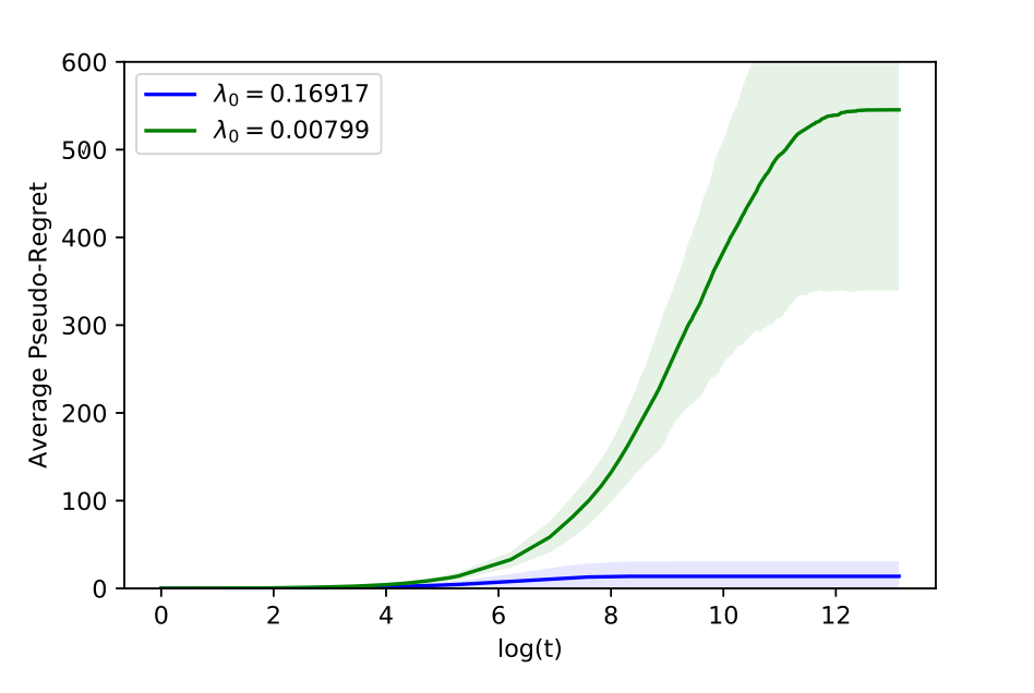
(a) Uniform context arrivals.
Refer to caption
(b) Uniform context arrivals with different context diversity.
(c) General context arrivals.
Figure 1: Pseudo-regret over log⁡T\log T. Shaded area indicates twice the standard deviation.

For each algorithm, we randomly pick one out of those four contexts with probability 1/41/4 each time, and add i.i.d. noise according to a standard Gaussian distribution 𝒩⁡(0,1)\mathcal{N}(0,1) to generate the reward. We run the simulation 100 times for each algorithm over 500,000 time slots. The sample average pseudo regrets are plotted in Fig. 1(a), where the pseudo regret is obtained by replacing yty_{t} in the definition of regret by r⁡(at,ct)r(a_{t},c_{t}), and the shaded area corresponds to twice of the standard deviation. As we expect, LinUCB-d with the same choice of αt\alpha_{t} behaves exactly the same as LinUCB, and shows bounded regret. However, the greedy algorithm and UCB do not achieve constant regret. This indicates the following: First, the pure exploitation strategy does not work well in this case. This is because the selected parameters do not satisfy the covariate diversity defined in Bastani et al., 2017. The covariate diversity in Bastani et al., 2017 requires that the correlation matrix of the feature vectors lying in any half space is positive definite. It requires that there are feature vectors at least in any half space. Since the feature vectors in our example only lie in the first orthant, the covariate diversity condition is not satisfied and hence the greedy approach does not work well. Second, treating each context individually does not utilize the information obtained under other contexts about the same arm, thus cannot leverage the diversity of context to reduce the regret.

Next, we evaluate how λ0\lambda_{0} affects the regrets. We modify the feature vectors associated with contexts 2 and 3 while keeping the rest parameters the same. Specifically, we let 𝐱⁡(1,2)=(0.45,0.65)⊺\mathbf{x}(1,2)=(0.45,0.65)^{\intercal}, 𝐱⁡(1,3)=(0.55,0.35)⊺\mathbf{x}(1,3)=(0.55,0.35)^{\intercal}, 𝐱⁡(2,2)=(0.3,0.5)⊺\mathbf{x}(2,2)=(0.3,0.5)^{\intercal}, 𝐱⁡(2,3)=(0.7,0.5)⊺\mathbf{x}(2,3)=(0.7,0.5)^{\intercal}. Compared with the previous setting, λ0\lambda_{0} increases from 0.007990.00799 to 0.169170.16917, while the reward gap Δ\Delta stays approximately the same. Intuitively, the basis vectors for each arm now point to more perpendicular directions and are more diverse in this sense. As indicated in Fig. 1(b), the increased diversity leads to much faster convergence and lower regret.

6.2 General Context Arrivals

In this part, we investigate the performance of LinUCB-d with a more general context distribution. We first randomly generate parameter vectors in ℝ4\mathbb{R}^{4} for 5 arms under the constraint that ‖𝜽⁡(a)‖2=10\|\bm{\theta}(a)\|_{2}=10. Thus, the arms are randomly located on a sphere in ℝ4\mathbb{R}^{4} with radius 10, which ensures that each of them can be optimal under certain contexts. For the feature vectors, we randomly draw 𝐱⁡(a,ct)∈[0,1]4\mathbf{x}(a,c_{t})\in[0,1]^{4} for a∈{1,2,3,4,5}a\in\{1,2,3,4,5\} at each time tt and make sure the reward gap condition in Assumption 1.2 is satisfied. We set Δ=0.5\Delta=0.5 throughout the simulation. The contexts are drawn from a continuous set which includes infinite many contexts.

We only compare LinUCB-d with greedy LinUCB under this setup. This is because UCB for individual contexts cannot be run without recurring contexts, and LinUCB with the same αt\alpha_{t} behaves the same as linUCB-d. The sample average pseudo regrets are plotted in Fig. 1(c). As we observe, LinUCB-d still achieves constant regret, while the greedy algorithm does not converge.

7 Related Work

The model considered in this paper falls in the contextual bandits framework. In the contextual MAB setting, the learner repeatedly takes one of KK actions in response to the observed context (Auer, 2003). Efficient exploration based on instantaneous context is of critical importance for contextual bandit algorithms to achieve small learning regret. The strongest known results (Auer, 2003; Langford and Zhang, 2008; McMahan and Streeter, 2009; Beygelzimer et al., 2011; Dudík et al., 2011; Agarwal et al., 2014) achieve an optimal regret after TT rounds of O⁡(K​T)O(\sqrt{KT}) with high probability.

More specifically, our reward model is similar to that of linear contextual bandits in the literature. This setting is first introduced in Auer, 2003 through the LinRel algorithm and is subsequently improved through the OFUL algorithm in Dani et al., 2008 and the LinUCB algorithm in Li et al., 2010. Rusmevichientong and Tsitsiklis, 2010 extend the work of Dani et al., 2008 by considering both optimistic and explore-then-commit strategies. It is shown in Abbasi-Yadkori et al., 2011 that the regret can be upper bounded by O⁡(d​T)O(d\sqrt{T}), where dd is the dimension of the context. A modified version of LinUCB, named SupLinUCB, is considered in Chu et al., 2011, and shown to achieve O⁡(d​T)O(\sqrt{dT}) regret. Later, Valko et al., 2013 mix LinUCB and SupLinUCB with kernel functions and propose an algorithm to further reduce the regret to O⁡(d~​T)O(\sqrt{\tilde{d}T}), where d~\tilde{d} is the effective dimension of the kernel feature space. This line of literature typically allows for arbitrary (adversarial) context sequences, and the O⁡(T)O(\sqrt{T}) regret persists.

Recently, a few works start to take the diversity in contexts into consideration. Goldenshluger and Zeevi, 2013 introduce a notion of diversity similar to Assumption 1.5 to a two-armed linear bandits setting. They show that the regret scales in O⁡(log⁡T)O(\log T) when a margin condition is satisfied, where the contribution from the “large-margin” covariates scales in O⁡(log⁡T)O(\log T). Bastani and Bayati, 2015 generalize the notation to a so called “compatibility condition” in a contextual linear bandits model with high-dimensional covariates, and investigate a LASSO based approach. They show that the regret can be bounded by a polynomial of log⁡T\log T under the margin condition. The O⁡(log⁡T)O(\log T) regret persists for error events associated with large-margin covariate vectors. In contrast, we show that a bounded regret can be achieved, by leveraging the geometric interpretation of the diversity condition and the reward gap condition.

Bastani et al., 2017 propose a concept called covariate diversity, which requires that the correlation matrix of the covariate vectors lying in any half space is positive definite. Under this condition, it shows that the exploration-free greedy algorithm is near-optimal for a two-armed bandit under the stochastic setting and achieves regret in O⁡(log⁡T)O(\log T). A perturbed adversarial setting with a similar notion of diversity is studied in Kannan et al., 2018. It shows that greedy algorithms can achieve regrets in O⁡(d​T)O(\sqrt{dT}). We note that such condition is stronger than Assumption 1.5. As illustrated through simulations in Section 6, a greedy strategy may not work well under our setting, due to the difference between the diversity definitions.

8 Conclusions

The main purpose of this paper was to study the impact of context diversity on the learning performance in stochastic linear contextual bandits. We have shown that, by adding an assumption that the context arrivals satisfy some diversity conditions, it is possible to significantly reduce the learning regret of contextual bandits. We proposed an algorithm called LinUCB-d and showed that when the diversity assumption is satisfied, the expected regret can in fact be upper bounded by a constant. This study illustrates the power of incorporating structure in the contexts to the bandit problem. It is of interest to evaluate whether other structures of the context can be similarly considered, and what their impacts would be. Another interesting problem is to study the impact of context diversity in other settings, such as the perturbed adversarial setting (Kannan et al., 2018).

Acknowledgements

JY acknowledges the support from U.S. National Science Foundation under Grant ECCS-1650299.

References

  • Abbasi-Yadkori et al., (2011) Abbasi-Yadkori, Y., Pál, D., and Szepesvári, C. (2011). Improved algorithms for linear stochastic bandits. In Proceedings of the 24th International Conference on Neural Information Processing Systems, pages 2312–2320.
  • Agarwal et al., (2014) Agarwal, A., Hsu, D., Kale, S., Langford, J., Li, L., and Schapire, R. E. (2014). Taming the monster: A fast and simple algorithm for contextual bandits. In In Proceedings of the 31st International Conference on Machine Learning, pages 1638–1646.
  • Agrawal and Goyal, (2012) Agrawal, S. and Goyal, N. (2012). Analysis of Thompson sampling for the multi-armed bandit problem. In Conference on Learning Theory, pages 39–1.
  • Agrawal and Goyal, (2013) Agrawal, S. and Goyal, N. (2013). Further optimal regret bounds for Thompson sampling. In Artificial Intelligence and Statistics, pages 99–107.
  • Auer, (2003) Auer, P. (2003). Using confidence bounds for exploitation-exploration trade-offs. J. Mach. Learn. Res., 3:397–422.
  • Auer et al., (2002) Auer, P., Cesa-Bianchi, N., and Fischer, P. (2002). Finite-time analysis of the multiarmed bandit problem. Machine learning, 47(2-3):235–256.
  • Bastani and Bayati, (2015) Bastani, H. and Bayati, M. (2015). Online decision-making with high-dimensional covariates. SSRN Electronic Journal.
  • Bastani et al., (2017) Bastani, H., Bayati, M., and Khosravi, K. (2017). Mostly exploration-free algorithms for contextual bandits. CoRR, abs/1704.09011.
  • Beygelzimer et al., (2011) Beygelzimer, A., Langford, J., Li, L., Reyzin, L., and Schapire, R. (2011). Contextual bandit algorithms with supervised learning guarantees. In Proceedings of the 14th International Conference on Artificial Intelligence and Statistics, pages 19–26, Fort Lauderdale, FL, USA.
  • Bubeck and Cesa-Bianchi, (2012) Bubeck, S. and Cesa-Bianchi, N. (2012). Regret analysis of stochastic and nonstochastic multi-armed bandit problems. Foundations and Trends® in Machine Learning, 5(1):1–122.
  • Chen and Xu, (2019) Chen, L. and Xu, J. (2019). Budget-constrained edge service provisioning with demand estimation via bandit learning. IEEE Journal on Selected Areas in Communications, 37(10):2364–2376.
  • Chu et al., (2011) Chu, W., Li, L., Reyzin, L., and Schapire, R. E. (2011). Contextual bandits with linear payoff functions. In AISTATS, volume 15, pages 208–214.
  • Dani et al., (2008) Dani, V., Hayes, T. P., and Kakade, S. M. (2008). Stochastic linear optimization under bandit feedback. In 21st Annual Conference on Learning Theory - COLT, pages 355–366.
  • Dudík et al., (2011) Dudík, M., Hsu, D. J., Kale, S., Karampatziakis, N., Langford, J., Reyzin, L., and Zhang, T. (2011). Efficient optimal learning for contextual bandits. CoRR, abs/1106.2369.
  • Goldenshluger and Zeevi, (2013) Goldenshluger, A. and Zeevi, A. (2013). A linear response bandit problem. Stoch. Syst., 3(1):230–261.
  • Kannan et al., (2018) Kannan, S., Morgenstern, J. H., Roth, A., Waggoner, B., and Wu, Z. S. (2018). A smoothed analysis of the greedy algorithm for the linear contextual bandit problem. In Advances in Neural Information Processing Systems 31, pages 2227–2236.
  • Lai and Robbins, (1985) Lai, T. L. and Robbins, H. (1985). Asymptotically efficient adaptive allocation rules. Advances in applied mathematics, 6(1):4–22.
  • Langford and Zhang, (2008) Langford, J. and Zhang, T. (2008). The epoch-greedy algorithm for multi-armed bandits with side information. In Advances in Neural Information Processing Systems, pages 817–824.
  • Lattimore and Szepesvári, (2019) Lattimore, T. and Szepesvári, C. (2019). Bandit Algorithms. Cambridge University Press (preprint).
  • Li et al., (2010) Li, L., Chu, W., Langford, J., and Schapire, R. E. (2010). A contextual-bandit approach to personalized news article recommendation. In Proceedings of the 19th International Conference on World Wide Web, pages 661–670.
  • McMahan and Streeter, (2009) McMahan, H. B. and Streeter, M. J. (2009). Tighter bounds for multi-armed bandits with expert advice. In COLT.
  • Rusmevichientong and Tsitsiklis, (2010) Rusmevichientong, P. and Tsitsiklis, J. N. (2010). Linearly parameterized bandits. Math. Oper. Res., 35:395–411.
  • Valko et al., (2013) Valko, M., Korda, N., Munos, R., Flaounas, I., and Cristianini, N. (2013). Finite-time analysis of kernelised contextual bandits. In Proceedings of the 29th Conference on Uncertainty in Artificial Intelligence, pages 654–663.
 

Supplementary Material: Stochastic Linear Contextual Bandits with Diverse Contexts


Weiqiang Wu          Jing Yang          Cong Shen

London Stock Exchange          The Pennsylvania State University          University of Virginia

Appendix A Proof of Proposition 1

For the constrained convex optimization problem in (6), the corresponding Lagrangian can be formulated as

ℒ⁡(𝜷,λ)\displaystyle\mathcal{L}(\bm{\beta},\lambda) =𝜷⊺​𝐍t−1​(a)​𝜷+(𝐱⁡(a,ct)−𝐗t​(a)​𝜷)⊺​𝝀,\displaystyle=\bm{\beta}^{\intercal}\mathbf{N}^{-1}_{t}(a)\bm{\beta}+\left(\mathbf{x}(a,{c_{t}})-\mathbf{X}_{t}(a)\bm{\beta}\right)^{\intercal}\bm{\lambda}, (10)

where 𝝀∈ℝd\bm{\lambda}\in{\mathbb{R}^{d}} is the Lagrangian multiplier vector.

Taking derivative with respect to 𝜷\bm{\beta}, we have

𝐍t−1​(a)​𝜷−𝐗t⊺​(a)​𝝀=0,\displaystyle\mathbf{N}^{-1}_{t}(a)\bm{\beta}-\mathbf{X}_{t}^{\intercal}(a)\bm{\lambda}=0, (11)

i.e.,

𝜷=𝐍t​(a)​𝐗t⊺​(a)​𝝀.\displaystyle\bm{\beta}=\mathbf{N}_{t}(a)\mathbf{X}_{t}^{\intercal}(a)\bm{\lambda}. (12)

Then, to satisfy the first constraint in (6), we have

𝐱⁡(a,ct)=𝐗t​(a)​𝜷=𝐗t​(a)​𝐍t​(a)​𝐗t⊺​(a)​𝝀,\displaystyle\mathbf{x}(a,{c_{t}})=\mathbf{X}_{t}(a)\bm{\beta}=\mathbf{X}_{t}(a)\mathbf{N}_{t}(a){\mathbf{X}_{t}^{\intercal}(a)}\bm{\lambda}, (13)

which implies that

𝝀=[𝐗t​(a)​𝐍t​(a)​𝐗t⊺​(a)]−1​𝐱​(a,ct):=𝐕t−1​(a)​𝐱​(a,ct).\displaystyle\bm{\lambda}=\left[\mathbf{X}_{t}(a)\mathbf{N}_{t}(a){\mathbf{X}_{t}^{\intercal}(a)}\right]^{-1}\mathbf{x}(a,{c_{t}}):=\mathbf{V}^{-1}_{t}(a)\mathbf{x}(a,{c_{t}}). (14)

Note that the definitions of 𝐗t​(a)\mathbf{X}_{t}(a) and 𝐍t​(a)\mathbf{N}_{t}(a) ensure that 𝐕t​(a)\mathbf{V}_{t}(a) is positive definite and invertible for every tt.

Plugging (14) into (12), we have

𝜷=𝐍t​(a)​𝐗t⊺​(a)​𝐕t−1​(a)​𝐱​(a,ct),\bm{\beta}=\mathbf{N}_{t}(a)\mathbf{X}_{t}^{\intercal}(a)\mathbf{V}^{-1}_{t}(a)\mathbf{x}(a,{c_{t}}),

which is the unique optimal solution to the optimization problem in (6).

Appendix B One the Relationship between LinUCB-d and LinUCB

Major difference. One major difference between LinUCB-d and LinUCB (Li et al., 2010) is as follows: Under LinUCB, at each time tt, it will first estimate the true parameter of arm aa (i.e., 𝜽a\bm{\theta}_{a}) by solving a ridge regression and then use it to derive the UCB for the expected reward. The criterion to select the estimate is to minimize the penalized mean squared error in fitting the past observations; On the other hand, under LinUCB-d, the learner will directly estimate the expected reward through a linear combination of the rewards obtained when arm aa was pulled under all contexts. The criterion of selecting the estimate is to minimize the uncertainty (or “variance") of the estimation. It avoids the intermediate step of trying to estimate 𝜽a\bm{\theta}_{a} first in LinUCB.

Essential equivalence. Although linUCB-d and linUCB view the problem from different angles, they actually produce the same estimate on the expected reward and confidence bound at every time tt under the same realizations of context arrivals and rewards, as shown below.

Based on (12), (13) and (14), the estimated mean reward r^t​(a)\hat{r}_{t}(a) in Algorithm 1 can be alternatively expressed as

r^t​(a)\displaystyle\hat{r}_{t}(a) =𝐬t⊺​(a)​𝐗t⊺​(a)​𝝀=𝐬t⊺​(a)​𝐗t⊺​(a)​𝐕t−1​(a)​𝐱​(a,ct):=𝜽^t⊺​(a)​𝐱​(a,ct),\displaystyle=\mathbf{s}_{t}^{\intercal}(a){\mathbf{X}_{t}^{\intercal}(a)}\bm{\lambda}=\mathbf{s}_{t}^{\intercal}(a){\mathbf{X}_{t}^{\intercal}(a)}\mathbf{V}^{-1}_{t}(a)\mathbf{x}(a,{c_{t}}):=\hat{\bm{\theta}}^{\intercal}_{t}(a)\mathbf{x}(a,{c_{t}}),

where 𝜽^t​(a):=𝐕t−1​(a)​𝐗t​(a)​𝐬t​(a)\hat{\bm{\theta}}_{t}(a):=\mathbf{V}^{-1}_{t}(a)\mathbf{X}_{t}(a)\mathbf{s}_{t}(a). We can verify that this is exactly the estimate of 𝜽⁡(a)\bm{\theta}(a) obtained by applying the ridge regression with penalty factor l2l^{2} to the historical data {(𝐱⁡(aτ,cτ),yτ)}τ=1t−1\{(\mathbf{x}(a_{\tau},c_{\tau}),y_{\tau})\}_{\tau=1}^{t-1}.

Besides, for the σ^t​(a)\hat{\sigma}_{t}(a) in Algorithm 1, we have

σ^t​(a)\displaystyle\hat{\sigma}_{t}(a) =𝝀⊺​𝐗t​(a)​𝐍t​(a)​𝐗t⊺​(a)​𝝀=‖𝐱⁡(a,ct)‖𝐕t−1​(a),\displaystyle=\sqrt{\bm{\lambda}^{\intercal}\mathbf{X}_{t}(a)\mathbf{N}_{t}(a){\mathbf{X}_{t}^{\intercal}(a)}\bm{\lambda}}=\|\mathbf{x}(a,{c_{t}})\|_{\mathbf{V}^{-1}_{t}(a)}, (15)

where we follow the convention to denote 𝐱𝐕𝐱⊺\mathbf{x}\mathbf{V}\mathbf{x}^{\intercal} as ‖𝐱‖𝐕2\|\mathbf{x}\|^{2}_{\mathbf{V}}.

Thus, if we let l=1l=1, both r^t​(a)\hat{r}_{t}(a) and σ^t​(a)\hat{\sigma}_{t}(a) share the same form as the corresponding quantities in LinUCB. As a reformulation of LinUCB, LinUCB-d automatically inherits all properties of LinUCB.

Computation and analytical issues. Computationally LinUCB-d is the same as LinUCB if we first compute the Lagrangian multiplier in (14) through 𝐕t​(a)\mathbf{V}_{t}(a), which can be equivalently computed by summing 𝐱⁡(a,ct)​𝐱⊺​(a,ct)\mathbf{x}(a,c_{t})\mathbf{x}^{\intercal}(a,c_{t}) over the time slots when aa is pulled. The advantage of LinUCB-d as an alternative form of LinUCB is on the analytical side. The prediction uncertainty minimization nature shown in Proposition 1 gives us a unique angle to elucidate the impact of context diversity on the corresponding learning regret, as elaborated in Lemma 3, Lemma 4, Lemma 9 and Lemma 10.

Appendix C Proof of Theorem 1

In the following, we will derive regret bounds for those error events individually, and then assemble them together to obtain the regret bound in Theorem 1.

C.1 Bound the Regret over 𝒜T\mathcal{A}_{T}

First, based on Hoeffding’s inequality, and the independent and uniform arrival of contexts assumption, we have

ℙ[NFk(c)≤12​n⋅2k−1]≤exp(−2k−12​n2).\displaystyle\mathbb{P}\left[N_{F_{k}}(c)\leq\frac{1}{2n}\cdot 2^{k-1}\right]\leq\exp\left(-\frac{2^{k-1}}{2n^{2}}\right). (16)

Denote R⁡(𝒜T)R(\mathcal{A}_{T}) as the regret incurred over 𝒜T\mathcal{A}_{T}, and MM as the maximum per-step regret. Then,

𝔼⁡[R⁡(𝒜T)]\displaystyle\mathbb{E}[R(\mathcal{A}_{T})] ≤M∑k=2⌈log2⁡T⌉∑t∈Fk𝔼[𝟏{t∈𝒜T}]≤M∑k=1⌊log2⁡T⌋∑t∈Fk+1∑a,c∈𝒞¯aℙ[NFk(c)≤2k−12​n]\displaystyle\leq M\sum_{k=2}^{\lceil\log_{2}T\rceil}\sum_{t\in F_{k}}\mathbb{E}[\mathbf{1}\{t\in\mathcal{A}_{T}\}]\leq M\sum_{k=1}^{\lfloor\log_{2}T\rfloor}\sum_{t\in F_{k+1}}\sum_{a,c\in\bar{\mathcal{C}}_{a}}\mathbb{P}\left[N_{F_{k}}(c)\leq\frac{2^{k-1}}{2n}\right]
≤M​K​d​∑k=1⌊log2⁡T⌋∑t∈Fk+1exp⁡(−2k−12​n2)≤M​n​∑t=2∞exp⁡(−t8​n2)\displaystyle\leq MKd\sum_{k=1}^{\lfloor\log_{2}T\rfloor}\sum_{t\in F_{k+1}}\exp\left(-\frac{2^{k-1}}{2n^{2}}\right)\leq Mn\sum_{t=2}^{\infty}\exp\left(-\frac{t}{8n^{2}}\right) (17)
≤M​K​d​∫0∞exp⁡(−t8​n2)​⁡𝑑t=8​M​K​d​n2,\displaystyle\leq MKd\int_{0}^{\infty}\exp\left(-\frac{t}{8n^{2}}\right)\mathop{}\!\mathrm{d}t=8MKdn^{2}, (18)

where (17) follows from (16).

C.2 Bound the Regret over ℬT\mathcal{B}_{T}

First, we define 𝐬~t​(a)\tilde{\mathbf{s}}_{t}(a) and 𝐬¯t​(a)\bar{\mathbf{s}}_{t}(a) as follows:

𝐬~t​(a)\displaystyle\tilde{\mathbf{s}}_{t}(a) =[St​(a,1)−Nt​(a,1)​r​(a,1),…,St​(a,nt)−Nt​(a,nt)​r​(a,nt),𝟎d]⊺\displaystyle=[S_{t}(a,1)-N_{t}(a,1)r(a,1),\ldots,S_{t}(a,n_{t})-N_{t}(a,n_{t})r(a,n_{t}),\mathbf{0}_{d}]^{\intercal} (19)
𝐬¯t​(a)\displaystyle\bar{\mathbf{s}}_{t}(a) =[𝟎nt,−l​𝐞1⊺​𝜽​(a),…,−l​𝐞d⊺​𝜽​(a)]⊺.\displaystyle=[\mathbf{0}_{n_{t}},-l\mathbf{e}_{1}^{\intercal}\bm{\theta}(a),\ldots,-l\mathbf{e}_{d}^{\intercal}\bm{\theta}(a)]^{\intercal}. (20)

Intuitively, 𝐬~t​(a)\tilde{\mathbf{s}}_{t}(a) corresponds to the accumulated noise in the observations when arm aa is pulled under different contexts up to time tt, and 𝐬¯t​(a)\bar{\mathbf{s}}_{t}(a) corresponds to the bias contributed by the feature vectors associated with the dummy contexts, which were added to ensure the existence of the unique solution in (6) for every tt.

Then, the reward estimation error can be expressed as

r^t​(a)−r⁡(a,ct)\displaystyle\hat{r}_{t}(a)-r(a,c_{t}) =𝐬t⊺​(a)​𝐍t−1​(a)​𝜷t​(a)−𝜽⊺​(a)​𝐱​(a,ct)\displaystyle=\mathbf{s}_{t}^{\intercal}(a)\mathbf{N}_{t}^{-1}(a)\bm{\beta}_{t}(a)-\bm{\theta}^{\intercal}(a)\mathbf{x}(a,c_{t})
=𝐬t⊺​(a)​𝐍t−1​(a)​𝜷t​(a)−𝜽⊺​(a)​𝐗t​(a)​𝜷t​(a)\displaystyle=\mathbf{s}_{t}^{\intercal}(a)\mathbf{N}_{t}^{-1}(a)\bm{\beta}_{t}(a)-\bm{\theta}^{\intercal}(a)\mathbf{X}_{t}(a)\bm{\beta}_{t}(a) (21)
=(𝐬t​(a)−𝐍t​(a)​𝐗⊺​(a)​𝜽​(a))⊺​𝐍t−1​(a)​𝜷t​(a)\displaystyle=\left(\mathbf{s}_{t}(a)-\mathbf{N}_{t}(a)\mathbf{X}^{\intercal}(a)\bm{\theta}(a)\right)^{\intercal}\mathbf{N}_{t}^{-1}(a)\bm{\beta}_{t}(a)
:=(𝐬~t​(a)+𝐬¯t​(a))⊺​𝐗t⊺​(a)​𝝀,\displaystyle:=(\tilde{\mathbf{s}}_{t}(a)+\bar{\mathbf{s}}_{t}(a))^{\intercal}\mathbf{X}_{t}^{\intercal}(a)\bm{\lambda}, (22)

where (21) is due to the fact that 𝐱⁡(a,ct)=𝐗t​(a)​𝜷t​(a)\mathbf{x}(a,c_{t})=\mathbf{X}_{t}(a)\bm{\beta}_{t}(a) according to Proposition 1, and the 𝝀\bm{\lambda} in (22) is the Lagrangian multiplier involved in the proof of Proposition 1 in Appendix A and satisfies (11). In the following, we will bound the contribution from 𝐬¯t​(a)\bar{\mathbf{s}}_{t}(a) and 𝐬~t​(a)\tilde{\mathbf{s}}_{t}(a) in the estimation error, respectively.

We note that at any time tt, Nt​(a,c)=1N_{t}(a,c)=1 for c=nt+1,…,nt+dc=n_{t}+1,\ldots,n_{t}+d. Besides, according to (15) in Appendix B,

σ^t​(a)\displaystyle\hat{\sigma}_{t}(a) =𝝀⊺​𝐗t​(a)​𝐍t​(a)​𝐗t⊺​(a)​𝝀=‖𝐍t1/2​(a)​𝐗t⊺​(a)​𝝀‖2.\displaystyle=\sqrt{\bm{\lambda}^{\intercal}\mathbf{X}_{t}(a)\mathbf{N}_{t}(a){\mathbf{X}_{t}^{\intercal}(a)}\bm{\lambda}}=\|\mathbf{N}_{t}^{1/2}(a)\mathbf{X}_{t}^{\intercal}(a)\bm{\lambda}\|_{2}.

Thus,

|𝐬¯t⊺​(a)​𝐗t⊺​(a)​𝝀|\displaystyle|\bar{\mathbf{s}}_{t}^{\intercal}(a)\mathbf{X}_{t}^{\intercal}(a)\bm{\lambda}| =|𝐬¯t⊺​(a)​𝐍t1/2​(a)​𝐗t⊺​(a)​𝝀|\displaystyle=|\bar{\mathbf{s}}_{t}^{\intercal}(a)\mathbf{N}_{t}^{1/2}(a)\mathbf{X}_{t}^{\intercal}(a)\bm{\lambda}| (23)
≤‖𝐬¯t⊺​(a)‖2⋅‖𝐍t1/2​(a)​𝐗t⊺​(a)​𝝀‖2\displaystyle\leq\|\bar{\mathbf{s}}_{t}^{\intercal}(a)\|_{2}\cdot\|\mathbf{N}_{t}^{1/2}(a)\mathbf{X}_{t}^{\intercal}(a)\bm{\lambda}\|_{2} (24)
=‖𝜽⁡(a)‖2​σ^t​(a)≤l​s​σ^t​(a),\displaystyle=\|\bm{\theta}(a)\|_{2}\hat{\sigma}_{t}(a)\leq ls\hat{\sigma}_{t}(a), (25)

where (24) follows from the Cauchy-Schwarz inequality.

Before we proceed to bound 𝐬~t⊺​(a)​𝐗t⊺​(a)​𝝀\tilde{\mathbf{s}}_{t}^{\intercal}(a)\mathbf{X}_{t}^{\intercal}(a)\bm{\lambda}, we first introduce the following notations. Recall that 𝐕t​(a):=𝐗t​(a)​𝐍t​(a)​𝐗t⊺​(a)\mathbf{V}_{t}(a):=\mathbf{X}_{t}(a)\mathbf{N}_{t}(a)\mathbf{X}_{t}^{\intercal}(a). Let 𝐕t1/2​(a)\mathbf{V}_{t}^{1/2}(a) be its square root, i.e., 𝐕t1/2​(a)​𝐕t1/2​(a)=𝐕t​(a)\mathbf{V}_{t}^{1/2}(a)\mathbf{V}_{t}^{1/2}(a)=\mathbf{V}_{t}(a). Let 𝐕~t​(a):=∑c=1nNt​(a,c)​𝐱​(a,c)​𝐱⊺​(a,c)\tilde{\mathbf{V}}_{t}(a):=\sum_{c=1}^{n}N_{t}(a,c)\mathbf{x}(a,c)\mathbf{x}^{\intercal}(a,c), 𝐕0:=l2​𝐈\mathbf{V}_{0}:=l^{2}\mathbf{I}. Then, 𝐕t​(a)=𝐕~t​(a)+𝐕0\mathbf{V}_{t}(a)=\tilde{\mathbf{V}}_{t}(a)+\mathbf{V}_{0}. We have

|𝐬~t⊺​(a)​𝐗t⊺​(a)​𝝀|\displaystyle|\tilde{\mathbf{s}}_{t}^{\intercal}(a)\mathbf{X}_{t}^{\intercal}(a)\bm{\lambda}| =|𝐬~t⊺(a)𝐗t⊺(a)𝐕t−1/2(a)𝐕t1/2(a)𝝀|\displaystyle=|\tilde{\mathbf{s}}_{t}^{\intercal}(a)\mathbf{X}_{t}^{\intercal}(a)\mathbf{V}_{t}^{-1/2}(a)\mathbf{V}_{t}^{1/2}(a)\bm{\lambda}|
≤‖𝐬~t⊺​(a)​𝐗t⊺​(a)‖𝐕t−1​(a)​‖𝐕t1/2​(a)​𝝀‖2\displaystyle\leq\|\tilde{\mathbf{s}}_{t}^{\intercal}(a)\mathbf{X}_{t}^{\intercal}(a)\|_{\mathbf{V}_{t}^{-1}(a)}\|\mathbf{V}_{t}^{1/2}(a)\bm{\lambda}\|_{2} (26)
=‖𝐬~t⊺​(a)​𝐗t⊺​(a)‖𝐕t−1​(a)​σ^t​(a).\displaystyle=\|\tilde{\mathbf{s}}_{t}^{\intercal}(a)\mathbf{X}_{t}^{\intercal}(a)\|_{\mathbf{V}_{t}^{-1}(a)}\hat{\sigma}_{t}(a). (27)

We then adopt the Laplace method (Lattimore and Szepesvári, 2019) to bound ‖𝐬~t⊺​(a)​𝐗t⊺​(a)‖𝐕t−1​(a)\|\tilde{\mathbf{s}}_{t}^{\intercal}(a)\mathbf{X}_{t}^{\intercal}(a)\|_{\mathbf{V}_{t}^{-1}(a)} as follows.

Lemma 1

Denote Mt​(𝐮):=exp⁡(𝐬~t⊺​(a)​𝐗t⊺​(a)​𝐮−12​𝐮⊺​𝐕~t​(a)​𝐮)M_{t}(\mathbf{u}):=\exp\left(\tilde{\mathbf{s}}_{t}^{\intercal}(a)\mathbf{X}_{t}^{\intercal}(a)\mathbf{u}-\frac{1}{2}\mathbf{u}^{\intercal}\tilde{\mathbf{V}}_{t}(a)\mathbf{u}\right) for any 𝐮\mathbf{u}. Let h⁡(𝐮)h(\mathbf{u}) be a probability measure over ℝd\mathbb{R}^{d}. Then, M¯t:=𝔼h​[Mt​(𝐮)]\bar{M}_{t}:=\mathbb{E}_{h}[M_{t}(\mathbf{u})] is a super martingale with M¯0=1\bar{M}_{0}=1.

Proof.

First, we note that Mt​(𝐮)−Mt−1​(𝐮)M_{t}(\mathbf{u})-M_{t-1}(\mathbf{u}) equals zero if arm aa is not pulled at time tt. Then, for any fixed 𝐮\mathbf{u}, we have

𝔼⁡[Mt​(𝐮)∣ℱt−1]\displaystyle\mathbb{E}[M_{t}(\mathbf{u})\mid\mathcal{F}_{t-1}]
=𝔼⁡[exp⁡(𝐬~t⊺​(a)​𝐗t⊺​(a)​𝐮−12​𝐮⊺​𝐕~t​(a)​𝐮)|ℱt−1]\displaystyle=\mathbb{E}\left[\exp\left(\tilde{\mathbf{s}}_{t}^{\intercal}(a)\mathbf{X}_{t}^{\intercal}(a)\mathbf{u}-\frac{1}{2}\mathbf{u}^{\intercal}\tilde{\mathbf{V}}_{t}(a)\mathbf{u}\right)\middle|\mathcal{F}_{t-1}\right] (28)
=𝔼⁡[exp⁡((𝐬~t⊺​(a)−𝐬~t−1⊺​(a))​𝐗t⊺​(a)​𝐮−12​𝐮⊺​(𝐕~t​(a)−𝐕~t−1​(a))​𝐮)]​Mt−1​(𝐮)\displaystyle=\mathbb{E}\left[\exp\left(\left(\tilde{\mathbf{s}}_{t}^{\intercal}(a)-\tilde{\mathbf{s}}_{t-1}^{\intercal}(a)\right)\mathbf{X}_{t}^{\intercal}(a)\mathbf{u}-\frac{1}{2}\mathbf{u}^{\intercal}\left(\tilde{\mathbf{V}}_{t}(a)-\tilde{\mathbf{V}}_{t-1}(a)\right)\mathbf{u}\right)\right]M_{t-1}(\mathbf{u}) (29)

Based on the definition of 𝐬~t\tilde{\mathbf{s}}_{t} in (27), 𝐬~t⊺​(a)−𝐬~t−1⊺​(a)\tilde{\mathbf{s}}_{t}^{\intercal}(a)-\tilde{\mathbf{s}}_{t-1}^{\intercal}(a) equals ηt​𝐞c⊺\eta_{t}\mathbf{e}^{\intercal}_{c} if at=a,ct=ca_{t}=a,c_{t}=c, and zero otherwise; Similarly, for 𝐕~t​(a)−𝐕~t−1​(a)\tilde{\mathbf{V}}_{t}(a)-\tilde{\mathbf{V}}_{t-1}(a), it equals 𝐱⁡(a,c)​𝐱⊺​(a,c)\mathbf{x}(a,c)\mathbf{x}^{\intercal}(a,c) if at=t,ct=ca_{t}=t,c_{t}=c, and zero otherwise. Therefore, if at≠aa_{t}\neq a,

𝔼⁡[exp⁡((𝐬~t⊺​(a)−𝐬~t−1⊺​(a))​𝐗⊺​(a)​𝐮−12​𝐮⊺​(𝐕~t​(a)−𝐕~t−1​(a))​𝐮)|at≠a]=1.\displaystyle\mathbb{E}\left[\exp\left(\left(\tilde{\mathbf{s}}_{t}^{\intercal}(a)-\tilde{\mathbf{s}}_{t-1}^{\intercal}(a)\right)\mathbf{X}^{\intercal}(a)\mathbf{u}-\frac{1}{2}\mathbf{u}^{\intercal}\left(\tilde{\mathbf{V}}_{t}(a)-\tilde{\mathbf{V}}_{t-1}(a)\right)\mathbf{u}\right)\middle|a_{t}\neq a\right]=1. (30)

If at=aa_{t}=a, ct=cc_{t}=c,

𝔼[exp((𝐬~t⊺(a)−𝐬~t−1⊺(a))𝐗⊺(a)𝐮−12𝐮⊺(𝐕~t(a)−𝐕~t−1(a))𝐮)|at=a,ct=c]\displaystyle\mathbb{E}\left[\exp\left(\left(\tilde{\mathbf{s}}_{t}^{\intercal}(a)-\tilde{\mathbf{s}}_{t-1}^{\intercal}(a)\right)\mathbf{X}^{\intercal}(a)\mathbf{u}-\frac{1}{2}\mathbf{u}^{\intercal}\left(\tilde{\mathbf{V}}_{t}(a)-\tilde{\mathbf{V}}_{t-1}(a)\right)\mathbf{u}\right)\middle|a_{t}=a,c_{t}=c\right] (31)
=𝔼⁡[exp⁡(ηt​𝐞c​𝐗⊺​(a)​𝐮−12​𝐮⊺​𝐱​(a,c)​𝐱⊺​(a,c)​𝐮)]\displaystyle=\mathbb{E}\left[\exp\left(\eta_{t}\mathbf{e}_{c}\mathbf{X}^{\intercal}(a)\mathbf{u}-\frac{1}{2}\mathbf{u}^{\intercal}\mathbf{x}(a,c)\mathbf{x}^{\intercal}(a,c)\mathbf{u}\right)\right] (32)
=𝔼⁡[exp⁡(ηt​𝐱⊺​(a,c)​𝐮)]⋅exp⁡(−12​𝐮⊺​𝐱​(a,c)​𝐱⊺​(a,c)​𝐮)\displaystyle=\mathbb{E}\left[\exp\left(\eta_{t}\mathbf{x}^{\intercal}(a,c)\mathbf{u}\right)\right]\cdot\exp\left(-\frac{1}{2}\mathbf{u}^{\intercal}\mathbf{x}(a,c)\mathbf{x}^{\intercal}(a,c)\mathbf{u}\right) (33)
≤exp⁡(12​(𝐱⊺​(a,c)​𝐮)2)⋅exp⁡(−12​𝐮⊺​𝐱​(a,c)​𝐱⊺​(a,c)​𝐮)=1\displaystyle\leq\exp\left(\frac{1}{2}\left(\mathbf{x}^{\intercal}(a,c)\mathbf{u}\right)^{2}\right)\cdot\exp\left(-\frac{1}{2}\mathbf{u}^{\intercal}\mathbf{x}(a,c)\mathbf{x}^{\intercal}(a,c)\mathbf{u}\right)=1 (34)

where the last inequality follows from Assumption 1.3 that ηt\eta_{t} is conditionally 1-subgaussian.

Combining (30)(34) with (29), for every fixed 𝐮\mathbf{u}, we have 𝔼⁡[Mt​(𝐮)∣ℱt−1]≤Mt−1​(𝐮)\mathbb{E}[M_{t}(\mathbf{u})\mid\mathcal{F}_{t-1}]\leq M_{t-1}(\mathbf{u}). Thus, {Mt​(𝐮)}t\{M_{t}(\mathbf{u})\}_{t} is a super-martingale, and

𝔼​[Mt​(𝐮)]\displaystyle\mathbb{E}[{M}_{t}(\mathbf{u})] ≤M0(𝐮)]=1.\displaystyle\leq{M}_{0}(\mathbf{u})]=1. (35)

Since this holds for every 𝐮\mathbf{u}, after taking expectation with respect to 𝐮\mathbf{u}, M¯t\bar{M}_{t} is a super-martingale as well. Thus, 𝔼⁡[M¯t]≤M¯0=1\mathbb{E}[\bar{M}_{t}]\leq\bar{M}_{0}=1. ∎

Lemma 2

Under Algorithm 1,

ℙ[∥𝐬~t⊺(a)𝐗t⊺(a)∥𝐕t−1​(a)≥2​u+log⁡det𝐕t​(a)det𝐕0]≤e−u.\displaystyle\mathbb{P}\left[\|\tilde{\mathbf{s}}_{t}^{\intercal}(a)\mathbf{X}_{t}^{\intercal}(a)\|_{\mathbf{V}^{-1}_{t}(a)}\geq\sqrt{2u+\log\frac{\det\mathbf{V}_{t}(a)}{\det\mathbf{V}_{0}}}\right]\leq e^{-u}.
Proof.

Assume hh is the probability density function of a Gaussian distribution 𝒩⁡(𝟎,𝐕0)\mathcal{N}(\mathbf{0},\mathbf{V}_{0}), i.e.,

h⁡(𝐮)=1(2​π)d​det𝐕0​exp⁡(−12​𝐮⊺​𝐕0​𝐮).h(\mathbf{u})=\frac{1}{\sqrt{(2\pi)^{d}\det\mathbf{V}_{0}}}\exp\left(-\frac{1}{2}\mathbf{u}^{\intercal}\mathbf{V}_{0}\mathbf{u}\right).

Then,

M¯t\displaystyle\bar{M}_{t} =∫ℝdMt​(𝐮)​h​(𝐮)​⁡𝑑𝐮\displaystyle=\int_{\mathbb{R}^{d}}M_{t}(\mathbf{u})h(\mathbf{u})\mathop{}\!\mathrm{d}\mathbf{u}
=1(2​π)d​det𝐕0−1​∫ℝdexp⁡(𝐬~t⊺​(a)​𝐗⊺​(a)​𝐮−12​𝐮⊺​𝐕~t​(a)​𝐮−12​𝐮⊺​𝐕0​𝐮)​⁡𝑑𝐮\displaystyle=\frac{1}{\sqrt{(2\pi)^{d}\det\mathbf{V}_{0}^{-1}}}\int_{\mathbb{R}^{d}}\exp\left(\tilde{\mathbf{s}}_{t}^{\intercal}(a)\mathbf{X}^{\intercal}(a)\mathbf{u}-\frac{1}{2}\mathbf{u}^{\intercal}\tilde{\mathbf{V}}_{t}(a)\mathbf{u}-\frac{1}{2}\mathbf{u}^{\intercal}\mathbf{V}_{0}\mathbf{u}\right)\mathop{}\!\mathrm{d}\mathbf{u}
=1(2​π)d​det𝐕0−1​∫ℝdexp⁡(𝐬~t⊺​(a)​𝐗⊺​(a)​𝐮−12​𝐮⊺​𝐕t​(a)​𝐮)​⁡𝑑𝐮\displaystyle=\frac{1}{\sqrt{(2\pi)^{d}\det\mathbf{V}_{0}^{-1}}}\int_{\mathbb{R}^{d}}\exp\left(\tilde{\mathbf{s}}_{t}^{\intercal}(a)\mathbf{X}^{\intercal}(a)\mathbf{u}-\frac{1}{2}\mathbf{u}^{\intercal}\mathbf{V}_{t}(a)\mathbf{u}\right)\mathop{}\!\mathrm{d}\mathbf{u}
=1(2​π)d​det𝐕0−1∫ℝdexp(𝐬~t⊺(a)𝐗⊺(a)𝐕t−1/2(a)𝐕t1/2(a)𝐮−12∥𝐮⊺𝐕t(a)∥𝐕t−1​(a))d𝐮\displaystyle=\frac{1}{\sqrt{(2\pi)^{d}\det\mathbf{V}_{0}^{-1}}}\int_{\mathbb{R}^{d}}\exp\left(\tilde{\mathbf{s}}_{t}^{\intercal}(a)\mathbf{X}^{\intercal}(a)\mathbf{V}^{-1/2}_{t}(a)\mathbf{V}^{1/2}_{t}(a)\mathbf{u}-\frac{1}{2}\|\mathbf{u}^{\intercal}\mathbf{V}_{t}(a)\|_{\mathbf{V}^{-1}_{t}(a)}\right)\mathop{}\!\mathrm{d}\mathbf{u}
=1(2​π)d​det𝐕0−1\displaystyle=\frac{1}{\sqrt{(2\pi)^{d}\det\mathbf{V}_{0}^{-1}}}
×∫ℝdexp⁡(12​‖𝐬~t⊺​(a)​𝐗⊺​(a)‖𝐕t−1​(a)2−12​‖𝐮⊺​𝐕t​(a)−𝐬~t⊺​(a)​𝐗⊺​(a)‖𝐕t−1​(a)2)​⁡𝑑𝐮\displaystyle\qquad\times\int_{\mathbb{R}^{d}}\exp\left(\frac{1}{2}\|\tilde{\mathbf{s}}_{t}^{\intercal}(a)\mathbf{X}^{\intercal}(a)\|^{2}_{\mathbf{V}^{-1}_{t}(a)}-\frac{1}{2}\|\mathbf{u}^{\intercal}\mathbf{V}_{t}(a)-\tilde{\mathbf{s}}_{t}^{\intercal}(a)\mathbf{X}^{\intercal}(a)\|_{\mathbf{V}^{-1}_{t}(a)}^{2}\right)\mathop{}\!\mathrm{d}\mathbf{u}
=det𝐕t−1​(a)det𝐕0−1​exp⁡(12​‖𝐬~t⊺​(a)​𝐗⊺​(a)‖𝐕t−1​(a)2)\displaystyle=\sqrt{\frac{\det\mathbf{V}^{-1}_{t}(a)}{\det{\mathbf{V}}^{-1}_{0}}}\exp\left(\frac{1}{2}\|\tilde{\mathbf{s}}_{t}^{\intercal}(a)\mathbf{X}^{\intercal}(a)\|^{2}_{\mathbf{V}^{-1}_{t}(a)}\right)
=exp⁡(12​‖𝐬~t⊺​(a)​𝐗⊺​(a)‖𝐕t−1​(a)2+12​log⁡det𝐕0det𝐕t​(a)).\displaystyle=\exp\left(\frac{1}{2}\|\tilde{\mathbf{s}}_{t}^{\intercal}(a)\mathbf{X}^{\intercal}(a)\|^{2}_{\mathbf{V}^{-1}_{t}(a)}+\frac{1}{2}\log\frac{\det\mathbf{V}_{0}}{\det\mathbf{V}_{t}(a)}\right).

Therefore, according to Lemma 1, we have

ℙ[∥𝐬~t⊺(a)𝐗t⊺(a)∥𝐕t−1​(a)≥2​u+log⁡det𝐕t​(a)det𝐕0]\displaystyle\mathbb{P}\left[\|\tilde{\mathbf{s}}_{t}^{\intercal}(a)\mathbf{X}_{t}^{\intercal}(a)\|_{\mathbf{V}^{-1}_{t}(a)}\geq\sqrt{2u+\log\frac{\det\mathbf{V}_{t}(a)}{\det{\mathbf{V}_{0}}}}\right]
=ℙ[12∥𝐬~t⊺(a)𝐗t⊺(a)∥𝐕t−1​(a)2+12logdet𝐕0det𝐕t​(a)≥u]\displaystyle=\mathbb{P}\left[\frac{1}{2}\|\tilde{\mathbf{s}}_{t}^{\intercal}(a)\mathbf{X}_{t}^{\intercal}(a)\|^{2}_{\mathbf{V}^{-1}_{t}(a)}+\frac{1}{2}\log\frac{\det{\mathbf{V}_{0}}}{\det\mathbf{V}_{t}(a)}\geq u\right]
≤e−u​𝔼​[M¯t]≤e−u.\displaystyle\leq e^{-u}\mathbb{E}[\bar{M}_{t}]\leq e^{-u}. (36)

∎

Next, we will provide a bound on det𝐕0det𝐕t​(a)\frac{\det\mathbf{V}_{0}}{\det\mathbf{V}_{t}(a)}. The definition of 𝐕0\mathbf{V}_{0} indicates that det𝐕0=l2​d\det{\mathbf{V}_{0}}=l^{2d}. For 𝐕t​(a)\mathbf{V}_{t}(a), we note that for any 𝐲∈ℝd\mathbf{y}\in\mathbb{R}^{d}, we have

𝐲⊺​𝐕t​(a)​𝐲\displaystyle\mathbf{y}^{\intercal}\mathbf{V}_{t}(a)\mathbf{y} =∑c=1nNt​(a,c)​𝐲⊺​𝐱​(a,c)​𝐱⊺​(a,c)​𝐲+l2​𝐲⊺​𝐲\displaystyle=\sum_{c=1}^{n}N_{t}(a,c)\mathbf{y}^{\intercal}\mathbf{x}(a,c)\mathbf{x}^{\intercal}(a,c)\mathbf{y}+l^{2}\mathbf{y}^{\intercal}\mathbf{y}
≤t​l2​‖𝐲‖22+l2​‖𝐲‖22=(t+1)​l2​‖𝐲‖22,\displaystyle\leq tl^{2}\|\mathbf{y}\|_{2}^{2}+l^{2}\|\mathbf{y}\|_{2}^{2}=(t+1)l^{2}\|\mathbf{y}\|_{2}^{2}, (37)

where the inequality follows from Assumption 1.1.

Eqn. (37) indicates that the maximum eigenvalue of 𝐕t​(a)\mathbf{V}_{t}(a) is upper bound by (t+1)​l2(t+1)l^{2}. Therefore, we have det𝐕t​(a)≤(l2+t​l2)d\det\mathbf{V}_{t}(a)\leq(l^{2}+tl^{2})^{d}, which implies that

log⁡det𝐕t​(a)det𝐕0≤d​log⁡(1+t).\displaystyle\log\frac{\det\mathbf{V}_{t}(a)}{\det\mathbf{V}_{0}}\leq d\log(1+t). (38)

Combining (38) with (22)(25)(27) and Lemma 2, we have

ℙ[|r^t(a)−r(a,ct)|≥(ls+2​u+d​log⁡(1+t))σ^t(a)]\displaystyle\mathbb{P}\left[|\hat{r}_{t}(a)-r(a,c_{t})|\geq\left(ls+\sqrt{2u+d\log(1+t)}\right)\hat{\sigma}_{t}(a)\right]
≤ℙ[∥𝐬~t⊺(a)𝐗⊺(a)∥𝐕t−1​(a)σ^t(a)≥2​u+d​log⁡(1+t)σ^t(a)]\displaystyle\leq\mathbb{P}\left[\|\tilde{\mathbf{s}}_{t}^{\intercal}(a)\mathbf{X}^{\intercal}(a)\|_{\mathbf{V}^{-1}_{t}(a)}\hat{\sigma}_{t}(a)\geq\sqrt{2u+d\log(1+t)}\hat{\sigma}_{t}(a)\right]
≤ℙ[∥𝐬~t⊺(a)𝐗⊺(a)∥𝐕t−1​(a)≥2​u+log⁡det𝐕t​(a)det𝐕0]≤e−u.\displaystyle\leq\mathbb{P}\left[\|\tilde{\mathbf{s}}_{t}^{\intercal}(a)\mathbf{X}^{\intercal}(a)\|_{\mathbf{V}^{-1}_{t}(a)}\geq\sqrt{2u+\log\frac{\det\mathbf{V}_{t}(a)}{\det\mathbf{V}_{0}}}\right]\leq e^{-u}. (39)

Set u=log⁡f⁡(t)u=\log f(t) and αt=l​s+(2+d)​log⁡f​(t)\alpha_{t}=ls+\sqrt{(2+d)\log f(t)}. When t>2t>2, f⁡(t)>1+tf(t)>1+t, therefore, (39) implies that

ℙ[|r^t(a)−r(a,ct)|≥αtσ^t(a)]≤1f⁡(t).\displaystyle\mathbb{P}\left[|\hat{r}_{t}(a)-r(a,c_{t})|\geq\alpha_{t}\hat{\sigma}_{t}(a)\right]\leq\frac{1}{f(t)}. (40)

Thus,

𝔼⁡[|ℬT|]\displaystyle\mathbb{E}[|\mathcal{B}_{T}|] ≤2+K​∑t=3∞1f⁡(t)≤2+2.5​K,𝔼⁡[R⁡(ℬT)]≤M​𝔼​[|ℬT|]≤M⁡(2+2.5​K).\displaystyle\leq 2+K\sum_{t=3}^{\infty}\frac{1}{f(t)}\leq 2+2.5K,\quad\mathbb{E}[R(\mathcal{B}_{T})]\leq M\mathbb{E}[|\mathcal{B}_{T}|]\leq M(2+2.5K). (41)

C.3 Bound the Regret over 𝒞T\mathcal{C}_{T}

Recall Bk:=|ℬT∩Fk|B_{k}:=|\mathcal{B}_{T}\cap F_{k}|, i.e., the number of bad estimates in frame kk. Then, according to Markov’s inequality, we have

ℙ[Bk≥2k−14​n]\displaystyle\mathbb{P}\left[B_{k}\geq\frac{2^{k-1}}{4n}\right] ≤𝔼⁡[Bk]​4​n2k−1.\displaystyle\leq\frac{\mathbb{E}[B_{k}]4n}{2^{k-1}}. (42)

The definitions of BkB_{k} and ℬT\mathcal{B}_{T} also imply that ∑k=1⌈log2⁡T⌉𝔼⁡[Bk]=𝔼⁡[ℬT].\sum_{k=1}^{\lceil\log_{2}T\rceil}\mathbb{E}[B_{k}]=\mathbb{E}[\mathcal{B}_{T}]. Therefore,

𝔼⁡[R⁡(𝒞T)]\displaystyle\mathbb{E}[R(\mathcal{C}_{T})] ≤M𝔼[|𝒞T|]=M∑k=1⌊log2⁡T⌋|Fk+1|⋅ℙ[Bk≥2k−14​n]\displaystyle\leq M{\mathbb{E}}[|\mathcal{C}_{T}|]=M\sum_{k=1}^{\lfloor\log_{2}T\rfloor}|F_{k+1}|\cdot\mathbb{P}\left[B_{k}\geq\frac{2^{k-1}}{4n}\right] (43)
≤M​∑k=1⌊log2⁡T⌋2k​𝔼⁡[Bk]​4​n2k−1≤8​n​M​𝔼​[|ℬT|]≤8​n​M​(2+2.5​K),\displaystyle\leq M\sum_{k=1}^{\lfloor\log_{2}T\rfloor}2^{k}\frac{\mathbb{E}[B_{k}]4n}{2^{k-1}}\leq 8nM\mathbb{E}[|\mathcal{B}_{T}|]\leq 8nM(2+2.5K), (44)

where (43) follows from the definition of 𝒞T\mathcal{C}_{T}, and (44) is due to (42) and (41).

C.4 Bound the Regret over 𝒟T\mathcal{D}_{T}

Let N¯t​(a,c)\bar{N}_{t}(a,c) be the total number of time slots before tt when arm aa is pulled under context cc, and all estimates are good, i.e., N¯t(a,c)=|{τ∣aτ=a,cτ=c,τ∉ℬt,1≤τ<t}|.\bar{N}_{t}(a,c)=|\{\tau\mid a_{\tau}=a,c_{\tau}=c,\tau\notin\mathcal{B}_{t},1\leq\tau<t\}|. We have the following observations.

Lemma 3

For any aa, c∉𝒞ac\notin\mathcal{C}_{a}, N¯t​(a,c)≤4​αt2Δ2\bar{N}_{t}(a,c)\leq\frac{{4}\alpha_{t}^{2}}{\Delta^{2}} for all tt.

Proof.

We first consider a time slot t∉ℬTt\notin\mathcal{B}_{T} at which a sub-optimal action ata_{t} is taken under ctc_{t}. Then, according to the LinUCB-d Algorithm, we must have

r^t​(at)+αt​σ^t​(at)≥r^t​(at∗)+αt​σ^t​(at∗).\displaystyle\hat{r}_{t}(a_{t})+\alpha_{t}\hat{\sigma}_{t}(a_{t})\geq\hat{r}_{t}(a^{*}_{t})+\alpha_{t}\hat{\sigma}_{t}(a^{*}_{t}). (45)

Besides, t∉ℬTt\notin\mathcal{B}_{T} implies that

|r^t​(at)−r⁡(at,ct)|\displaystyle|\hat{r}_{t}(a_{t})-r(a_{t},c_{t})| ≤αt​σ^t​(at),|r^t​(at∗)−r⁡(at∗,ct)|≤αt​σ^t​(at∗).\displaystyle\leq\alpha_{t}\hat{\sigma}_{t}(a_{t}),\quad|\hat{r}_{t}(a^{*}_{t})-r(a^{*}_{t},c_{t})|\leq\alpha_{t}\hat{\sigma}_{t}(a^{*}_{t}). (46)

Putting (45)(46) together, we have

r⁡(at,ct)+2​αt​σ^t​(at)≥r^t​(at)+αt​σ^t​(at)≥r^t​(at∗)+αt​σ^t​(at∗)≥r⁡(at∗,ct).\displaystyle r(a_{t},c_{t})+2\alpha_{t}\hat{\sigma}_{t}(a_{t})\geq\hat{r}_{t}(a_{t})+\alpha_{t}\hat{\sigma}_{t}(a_{t})\geq\hat{r}_{t}(a^{*}_{t})+\alpha_{t}\hat{\sigma}_{t}(a^{*}_{t})\geq r(a^{*}_{t},c_{t}). (47)

Therefore,

Δ≤r⁡(at∗,ct)−r⁡(at,ct)≤2​αt​σ^t​(at)=2​αt​𝜷t⊺​(at)​𝐍t−1​(at)​𝜷t​(at).\displaystyle\Delta\leq r(a^{*}_{t},c_{t})-r(a_{t},c_{t})\leq 2\alpha_{t}\hat{\sigma}_{t}(a_{t})=2\alpha_{t}\sqrt{\bm{\beta}_{t}^{\intercal}(a_{t})\mathbf{N}_{t}^{-1}(a_{t})\bm{\beta}_{t}(a_{t})}. (48)

Denote 𝜷~∈ℝnt+d\tilde{\bm{\beta}}\in\mathbb{R}^{n_{t}+d} as a unit vector whose ctc_{t}-th entry takes value 11. Then, when Nt​(at,ct)≠0N_{t}(a_{t},c_{t})\neq 0, 𝜷~\tilde{\bm{\beta}} satisfies the constraints in (6). According to Proposition 1, we must have

𝜷t⊺​(at)​𝐍t−1​(at)​𝜷t​(at)≤𝜷~⊺​(at)​𝐍t−1​(at)​𝜷~​(at)=1Nt​(at,ct)≤1N¯t​(at,ct).\displaystyle\bm{\beta}_{t}^{\intercal}(a_{t})\mathbf{N}_{t}^{-1}(a_{t})\bm{\beta}_{t}(a_{t})\leq\tilde{\bm{\beta}}^{\intercal}(a_{t})\mathbf{N}_{t}^{-1}(a_{t})\tilde{\bm{\beta}}(a_{t})=\frac{1}{N_{t}(a_{t},c_{t})}\leq\frac{1}{\bar{N}_{t}(a_{t},c_{t})}. (49)

Combining (48) and (49), we have

N¯t​(at,ct)\displaystyle\bar{N}_{t}(a_{t},c_{t}) ≤1𝜷t⊺​(at)​𝐍t−1​(at)​𝜷t​(at)≤4​αt2Δ2.\displaystyle\leq\frac{1}{\bm{\beta}_{t}^{\intercal}(a_{t})\mathbf{N}_{t}^{-1}(a_{t})\bm{\beta}_{t}(a_{t})}\leq\frac{4\alpha^{2}_{t}}{\Delta^{2}}. (50)

When Nt​(at,ct)=0N_{t}(a_{t},c_{t})=0, we must have N¯t​(at,ct)=0\bar{N}_{t}(a_{t},c_{t})=0, thus (50) is satisfied as well.

Hence, Lemma 3 holds for all time slots t∉ℬTt\notin\mathcal{B}_{T}. Since N¯t​(a,c)\bar{N}_{t}(a,c) is a step function for any fixed (a,c)(a,c) pair and αt\alpha_{t} monotonically increases in tt, Lemma 3 hold for all tt as well. ∎

Lemma 3 indicates that the total number of times that aa is pulled as a sub-optimal arm up to tt is bounded by O⁡(log⁡f⁡(t))O(\log f(t)). Based on this result, we will then show that the total number of times that aa is pulled as an optimal arm grows linearly in tt, as described in Lemma 4. Next, we utilize Lemma 4 to show the diminishing estimation uncertainty in Lemma 6, which eventually leads to the finite regret bound over 𝒟T\mathcal{D}_{T} in Theorem 4.

Lemma 4

For any aa, c∈𝒞ac\in\mathcal{C}_{a} and any time slot t∈𝒟Tt\in\mathcal{D}_{T}, we must have Nt​(a,c)≥t16​n−8​K​αt2Δ2N_{t}(a,c)\geq\frac{t}{16n}-\frac{8K\alpha_{t}^{2}}{\Delta^{2}}.

Proof.

Assume tt lies in the (k+1)(k+1)th time frame. Then, based on the definition of Nt​(a,c)N_{t}(a,c), we must have

Nt​(a,c)\displaystyle N_{t}(a,c) ≥NFk(a,c)=NFk(c)−∑b:b≠aNFk(b,c)≥2k−12​n−[Bk+∑b:b≠aN¯2k(b,c)]\displaystyle\geq N_{F_{k}}(a,c)=N_{F_{k}}(c)-\sum_{b:b\neq a}N_{F_{k}}(b,c)\geq\frac{2^{k-1}}{2n}-\Big[B_{k}+\sum_{b:b\neq a}\bar{N}_{2^{k}}(b,c)\Big] (51)
≥2k−12​n−2k−14​n−K​4​αt2Δ2≥t16​n−4​K​αt2Δ2,\displaystyle\geq\frac{2^{k-1}}{2n}-\frac{2^{k-1}}{4n}-K\frac{4\alpha_{t}^{2}}{\Delta^{2}}\geq\frac{t}{16n}-\frac{4K\alpha_{t}^{2}}{\Delta^{2}}, (52)

where (51) follows from the assumption that t∉𝒜Tt\notin\mathcal{A}_{T}, and (52) follows from the assumption that t∉𝒞Tt\notin\mathcal{C}_{T} and Lemma 3. ∎

Before we proceed, we introduce the following lemma.

Lemma 5

Let {ϕ1,ϕ2,…,ϕd}\{\phi_{1},\phi_{2},\ldots,\phi_{d}\} be a basis for ℝd\mathbb{R}^{d}, and Φ:=[ϕ1,ϕ2,…,ϕd]\Phi:=[\phi_{1},\phi_{2},\ldots,\phi_{d}]. Then, for any 𝐱∈ℝd\mathbf{x}\in\mathbb{R}^{d}, ‖𝐱‖2≤l\|\mathbf{x}\|_{2}\leq l, we can express it as 𝐱=Φ​𝛃\mathbf{x}=\Phi\bm{\beta}, where 𝛃∈ℝd\bm{\beta}\in\mathbb{R}^{d}, ‖𝛃‖1≤l​dλmin​(Φ⊺​Φ)\|\bm{\beta}\|_{1}\leq\frac{l\sqrt{d}}{\sqrt{\lambda_{\min}(\Phi^{\intercal}\Phi)}}.

Proof.

Since

l2≥‖𝐱‖22=𝜷⊺​Φ⊺​Φ​𝜷≥λmin​(Φ⊺​Φ)​𝜷⊺​𝜷≥λmin​(Φ⊺​Φ)​‖𝜷‖12d,\displaystyle l^{2}\geq\|\mathbf{x}\|_{2}^{2}=\bm{\beta}^{\intercal}\Phi^{\intercal}\Phi\bm{\beta}\geq\lambda_{\min}(\Phi^{\intercal}\Phi)\bm{\beta}^{\intercal}\bm{\beta}\geq\frac{\lambda_{\min}(\Phi^{\intercal}\Phi)\|\bm{\beta}\|_{1}^{2}}{d}, (53)

we have ‖𝜷‖1≤l​dλmin​(Φ⊺​Φ)\|\bm{\beta}\|_{1}\leq\frac{l\sqrt{d}}{\sqrt{\lambda_{\min}(\Phi^{\intercal}\Phi)}}. ∎

Lemma 6

For any arm a∈[K]a\in[K], any time slot t∈𝒟Tt\in\mathcal{D}_{T}, we must have 𝛃t⊺​(a)​𝐍t−1​(a)​𝛃t​(a)≤δ2t16​n−4​K​αt2Δ2\bm{\beta}_{t}^{\intercal}(a)\mathbf{N}_{t}^{-1}(a)\bm{\beta}_{t}(a)\leq\frac{\delta^{2}}{\frac{t}{16n}-\frac{4K\alpha_{t}^{2}}{\Delta^{2}}}, where δ:=l​d/λ0\delta:=l\sqrt{d/\lambda_{0}}.

Proof.

For any a∈[K],c∈𝒞a\in[K],c\in\mathcal{C}, let 𝜷¯​(a,c)\bar{\bm{\beta}}(a,c) be the solution to the following equation

𝐱⁡(a,c)=𝐗t​(a)​𝜷¯,𝜷¯​[c]=0, for ​c∉𝒞¯a.\displaystyle\mathbf{x}(a,c)=\mathbf{X}_{t}(a)\bar{\bm{\beta}},\quad\bar{\bm{\beta}}[c]=0,\mbox{ for }c\notin\bar{\mathcal{C}}_{a}. (54)

Note that we use 𝜷¯​[c]\bar{\bm{\beta}}[c] to denote the entry associated with context cc in 𝜷¯\bar{\bm{\beta}}.

Consider a time slot t∈𝒟Tt\in\mathcal{D}_{T}. Based on the definitions of the error events in Section 4, we note that all contexts in 𝒞¯a\bar{\mathcal{C}}_{a} must have appeared before time slot tt. Thus, 𝐗t​(a)\mathbf{X}_{t}(a) contains all columns in Φ¯a\bar{\Phi}_{a}. Therefore, 𝜷¯​(a,c)\bar{\bm{\beta}}(a,c) is simply the coefficient vector if we express 𝐱⁡(a,c)\mathbf{x}(a,c) as a linear combination of the feature vectors in Φ¯a\bar{\Phi}_{a}. The diversity assumption in Assumption 1.5 guarantees that there exists a unique solution 𝜷¯​(a,c)\bar{\bm{\beta}}(a,c) for each (a,c)(a,c) pair. Besides, Lemma 5 implies that ‖𝜷¯​(a,c)‖1≤l​dλmin​(Φ¯a⊺​Φ¯a)\|\bar{\bm{\beta}}(a,c)\|_{1}\leq\frac{l\sqrt{d}}{\sqrt{\lambda_{\min}(\bar{\Phi}_{a}^{\intercal}\bar{\Phi}_{a})}}.

Then, according to Proposition 1, Lemma 4 and Lemma 5, we must have

𝜷t⊺​(a)​𝐍t−1​(a)​𝜷t​(a)≤𝜷¯⊺​(a,ct)​𝐍t−1​(a)​𝜷¯​(a,ct)≤‖𝜷¯​(a,ct)‖12t16​n−4​K​αt2Δ2≤δ2t16​n−4​K​αt2Δ2,\displaystyle\bm{\beta}_{t}^{\intercal}(a)\mathbf{N}_{t}^{-1}(a)\bm{\beta}_{t}(a)\leq\bar{\bm{\beta}}^{\intercal}(a,c_{t})\mathbf{N}_{t}^{-1}(a)\bar{\bm{\beta}}(a,c_{t})\leq\frac{\|\bar{\bm{\beta}}(a,c_{t})\|_{1}^{2}}{\frac{t}{16n}-\frac{4K\alpha_{t}^{2}}{\Delta^{2}}}\leq\frac{\delta^{2}}{\frac{t}{16n}-\frac{4K\alpha_{t}^{2}}{\Delta^{2}}}, (55)

where the first inequality in (55) follows from Proposition 1, the second inequality follows from Lemma 4, and the last inequality follows from Lemma 5. ∎

We then have the following bound on 𝔼⁡[R⁡(𝒟T)]\mathbb{E}[R(\mathcal{D}_{T})].

Theorem 3

Let

t1=max⁡{384​(2+d)​n​(δ2+K)Δ2,10},t2=max⁡{t1​log⁡t1,exp⁡(12​l2​s22+d)}.t_{1}=\max\left\{\frac{384(2+d)n(\delta^{2}+K)}{\Delta^{2}},10\right\},\quad t_{2}=\max\left\{t_{1}\log t_{1},\exp\left(\frac{12l^{2}s^{2}}{2+d}\right)\right\}.

Then, under Algorithm 1,

𝔼⁡[R⁡(𝒟T)]≤t2​M=O⁡(d​n​(δ2+K)Δ2​log⁡d​n​(δ2+K)Δ2).\displaystyle\mathbb{E}[R(\mathcal{D}_{T})]\leq t_{2}M=O\left(\frac{dn(\delta^{2}+K)}{\Delta^{2}}\log\frac{dn(\delta^{2}+K)}{\Delta^{2}}\right).
Proof.

For any t≥t2t\geq t_{2}, we have

t≥exp⁡(12​l2​s22+d)≥exp⁡((2+3)2​l2​s22+d),\displaystyle t\geq\exp\left(\frac{12l^{2}s^{2}}{2+d}\right)\geq\exp\left(\frac{(\sqrt{2}+\sqrt{3})^{2}l^{2}s^{2}}{2+d}\right),

which implies that

l​s≤2+d​(3−2)​log⁡t.\displaystyle ls\leq\sqrt{2+d}(\sqrt{3}-\sqrt{2})\sqrt{\log t}. (56)

Meanwhile, since log⁡f⁡(t)≤2​log⁡t\log f(t)\leq 2\log t, combining with (56), we have

αt:=l​s+(2+d)​log⁡f​(t)≤3​(2+d)​log⁡t.\displaystyle\alpha_{t}:=ls+\sqrt{(2+d)\log f(t)}\leq\sqrt{3(2+d)\log t}. (57)

Since t2log⁡t2≥t1​log⁡t1log⁡(t1​log⁡t1)≥t12\frac{t_{2}}{\log t_{2}}\geq\frac{t_{1}\log t_{1}}{\log(t_{1}\log t_{1})}\geq\frac{t_{1}}{2}, for any t≥t2t\geq t_{2}, we have

tlog⁡t≥t12=192​(2+d)​n​(δ2+K)Δ2,\displaystyle\frac{t}{\log t}\geq\frac{t_{1}}{2}=\frac{192(2+d)n(\delta^{2}+K)}{\Delta^{2}}, (58)

i.e.,

t\displaystyle t >192​(2+d)​n​(δ2+K)Δ2​log⁡t≥64​n​(δ2+K)Δ2​αt2,\displaystyle>\frac{192(2+d)n(\delta^{2}+K)}{\Delta^{2}}\log t\geq\frac{64n(\delta^{2}+K)}{\Delta^{2}}\alpha_{t}^{2},

where the last inequality is due to (57).

Thus,

t16​n\displaystyle\frac{t}{16n} ≥4​αt2​δ2Δ2+4​K​αt2Δ2.\displaystyle\geq\frac{4\alpha_{t}^{2}\delta^{2}}{\Delta^{2}}+\frac{4K\alpha_{t}^{2}}{\Delta^{2}}. (59)

Rearranging the terms, we have

Δ2\displaystyle\Delta^{2} >4​αt2​δ2t16​n−4​K​αt2Δ2≥(2​αt​σ^t​(a))2,∀a∈[K],\displaystyle>\frac{4\alpha_{t}^{2}\delta^{2}}{\frac{t}{16n}-\frac{4K\alpha_{t}^{2}}{\Delta^{2}}}\geq(2\alpha_{t}\hat{\sigma}_{t}(a))^{2},\quad\forall a\in[K], (60)

where the last inequality follows from Lemma 6.

Since Δ≥2​αt​σ^t​(a)\Delta\geq 2\alpha_{t}\hat{\sigma}_{t}(a) for any t≥t2t\geq t_{2}, arm aa will not be pulled as a suboptimal arm at any time t∉ℬTt\notin\mathcal{B}_{T}, according to Eqn. (48). Therefore, 𝒟T\mathcal{D}_{T} can only include time indices before t2t_{2}. The expected regret over 𝒟T\mathcal{D}_{T} can thus be bounded by M​t2Mt_{2}. ∎

C.5 Put Everything Together

After obtaining bounds on the expected regret over 𝒜T\mathcal{A}_{T}, ℬT\mathcal{B}_{T}, 𝒞T\mathcal{C}_{T} and 𝒟T\mathcal{D}_{T}, we are ready to prove our main result in Theorem 1. We have

𝔼⁡[RT]\displaystyle\mathbb{E}[R_{T}] ≤𝔼⁡[R⁡(𝒜T)]+𝔼⁡[R⁡(ℬT)]+𝔼⁡[R⁡(𝒞T)]+𝔼⁡[R⁡(𝒟T)]\displaystyle\leq\mathbb{E}[R(\mathcal{A}_{T})]+\mathbb{E}[R(\mathcal{B}_{T})]+\mathbb{E}[R(\mathcal{C}_{T})]+\mathbb{E}[R(\mathcal{D}_{T})]
≤8​M​K​d​n2+(8​n+1)​M​(2+2.5​K)+t2​M\displaystyle\leq 8MKdn^{2}+(8n+1)M(2+2.5K)+t_{2}M (61)
=O⁡(K​d​n2+d​n​(K+δ2)Δ2​log⁡d​n​(K+δ2)Δ2).\displaystyle=O\left(Kdn^{2}+\frac{dn(K+\delta^{2})}{\Delta^{2}}\log\frac{dn(K+\delta^{2})}{\Delta^{2}}\right). (62)

We point out that the O⁡(exp⁡(12​l2​s22+d))O\left(\exp\left(\frac{12l^{2}s^{2}}{2+d}\right)\right) term from t2t_{2} is dropped in (62), since it mainly depends on the bounds on ‖𝜽⁡(a)‖2\|\bm{\theta}(a)\|_{2} and ‖𝐱⁡(a,c)‖2\|\mathbf{x}(a,c)\|_{2}, and does not scale with the system dimensions dd or KK.

Appendix D Proof of Theorem 2

Before we proceed, we will first introduce the following lemma, which will play a critical role in the analysis afterwards.

Lemma 7

Let {ϕ1,ϕ2,…,ϕd}\{\phi_{1},\phi_{2},\ldots,\phi_{d}\} be a basis for ℝd\mathbb{R}^{d}, and Φ:=[ϕ1,ϕ2,…,ϕd]\Phi:=[\phi_{1},\phi_{2},\ldots,\phi_{d}]. Let B⁡(ϕi,r)B(\phi_{i},r) be an ℓ2\ell_{2} ball centered at ϕi\phi_{i} with radius r<λmin​(Φ⊺​Φ)/dr<\sqrt{\lambda_{\min}(\Phi^{\intercal}\Phi)/d}, i.e., B⁡(ϕi,r):={𝐱∈ℝd∣‖𝐱−ϕi‖2≤r}B(\phi_{i},r):=\{\mathbf{x}\in\mathbb{R}^{d}\mid\|\mathbf{x}-\phi_{i}\|_{2}\leq r\}. Let ϕ^i\hat{\phi}_{i} be any vector lying in B⁡(ϕi,r)B(\phi_{i},r) and Φ^:=[ϕ^1,ϕ^2,…,ϕ^d]\hat{\Phi}:=[\hat{\phi}_{1},\hat{\phi}_{2},\ldots,\hat{\phi}_{d}]. Then, λmin​(Φ^⊺​Φ^)≥(λmin​(Φ⊺​Φ)−d​r)2\lambda_{\min}(\hat{\Phi}^{\intercal}\hat{\Phi})\geq(\sqrt{\lambda_{\min}(\Phi^{\intercal}\Phi)}-\sqrt{d}r)^{2}.

Proof.

Denote γi:=ϕ^i−ϕi\gamma_{i}:=\hat{\phi}_{i}-\phi_{i}. Then, based on the definition of ϕ^i\hat{\phi}_{i}, we have ‖γi‖2≤r\|\gamma_{i}\|_{2}\leq r. Let Γ=[γ1,γ2,…,γd]\Gamma=[\gamma_{1},\gamma_{2},\ldots,\gamma_{d}], and Γ⁡(j)\Gamma(j) be its jjth row. Then, for any 𝜷∈ℝd\bm{\beta}\in\mathbb{R}^{d},

‖Φ^​𝜷‖2\displaystyle\|\hat{\Phi}\bm{\beta}\|_{2} =‖Φ​𝜷+Γ​𝜷‖2≥‖Φ​𝜷‖2−‖Γ​𝜷‖2≥λmin​(Φ⊺​Φ)​‖𝜷‖2−∑j|Γ⁡(j)​𝜷|2\displaystyle=\left\|\Phi\bm{\beta}+\Gamma\bm{\beta}\right\|_{2}\geq\left\|\Phi\bm{\beta}\right\|_{2}-\left\|\Gamma\bm{\beta}\right\|_{2}\geq\sqrt{\lambda_{\min}(\Phi^{\intercal}\Phi)}\|\bm{\beta}\|_{2}-\sqrt{\sum_{j}\left|\Gamma(j)\bm{\beta}\right|^{2}} (63)
≥λmin​(Φ⊺​Φ)​‖𝜷‖2−∑j‖Γ(j)∥22∥𝜷‖22\displaystyle\geq\sqrt{\lambda_{\min}(\Phi^{\intercal}\Phi)}\|\bm{\beta}\|_{2}-\sqrt{\sum_{j}\left\|\Gamma(j)\|_{2}^{2}\|\bm{\beta}\right\|_{2}^{2}} (64)
=λmin​(Φ⊺​Φ)​‖𝜷‖2−‖𝜷‖2​∑i=1dγi⊺​γi\displaystyle=\sqrt{\lambda_{\min}(\Phi^{\intercal}\Phi)}\|\bm{\beta}\|_{2}-\|\bm{\beta}\|_{2}\sqrt{\sum_{i=1}^{d}\gamma_{i}^{\intercal}\gamma_{i}} (65)
≥(λmin​(Φ⊺​Φ)−d​r)​‖𝜷‖2,\displaystyle\geq\left(\sqrt{\lambda_{\min}(\Phi^{\intercal}\Phi)}-\sqrt{d}r\right)\|\bm{\beta}\|_{2}, (66)

where (63) follows from (53), and (64) follows from the Cauchy-Schwartz inequality; Rearranging the terms involved in the summation, we obtain (65), which can be further bounded by (66) due to the definition of B⁡(ϕi,r)B(\phi_{i},r).

Thus, the eigenvalues of Φ^⊺​Φ^\hat{\Phi}^{\intercal}\hat{\Phi} are lower bounded by (λmin​(Φ⊺​Φ)−d​r)2>0(\sqrt{\lambda_{\min}(\Phi^{\intercal}\Phi)}-\sqrt{d}r)^{2}>0. ∎

Remark: Lemma 7 implies that {ϕ^i}\{\hat{\phi}_{i}\} are linearly independent, thus forming a valid basis for ℝd\mathbb{R}^{d}.

D.1 Bound the Regret over 𝒜T\mathcal{A}_{T}

First, based on Hoeffding’s inequality, we have

ℙ[NFk(𝒞¯a(i))≤p2⋅2k−1]≤exp(−p22k−2).\displaystyle\mathbb{P}\left[N_{F_{k}}(\bar{\mathcal{C}}_{a}^{(i)})\leq\frac{p}{2}\cdot 2^{k-1}\right]\leq\exp\left(-p^{2}2^{k-2}\right). (67)

Recall that MM is the maximum per-step regret. Thus, by extending the proof in Appendix C.1, we have

𝔼⁡[R⁡(𝒜T)]≤M⁡(K​d)​∑t=2∞exp⁡(−p28​t)≤8​M​K​dp2.\displaystyle\mathbb{E}[R(\mathcal{A}_{T})]\leq M(Kd)\sum_{t=2}^{\infty}\exp\left(-\frac{p^{2}}{8}t\right)\leq\frac{8MKd}{p^{2}}. (68)

D.2 Bound the Regret over 𝒞T\mathcal{C}_{T}

According to Markov’s inequality, we have

ℙ[Bk≥p⋅2k−14]\displaystyle\mathbb{P}\left[B_{k}\geq\frac{p\cdot 2^{k-1}}{4}\right] ≤𝔼⁡[Bk]⋅4p⋅2k−1.\displaystyle\leq\frac{\mathbb{E}[B_{k}]\cdot 4}{p\cdot 2^{k-1}}. (69)

Therefore, by following similar steps in Appendix C.3, we have

𝔼⁡[R⁡(𝒞T)]\displaystyle\mathbb{E}[R(\mathcal{C}_{T})] ≤8​Mp​𝔼​[ℬT]≤8​M​(2+2.5​K)p.\displaystyle\leq\frac{8M}{p}\mathbb{E}[\mathcal{B}_{T}]\leq\frac{8M(2+2.5K)}{p}. (70)

D.3 Bound the Regret over 𝒟T\mathcal{D}_{T}

Before we proceed, we first state an adapted version of the celebrated elliptical potential lemma below, which will play a key role to analysis afterwards.

Lemma 8 (Elliptical Potential (Lattimore and Szepesvári, 2019))

Let 𝐕0\mathbf{V}_{0} be positive definite and 𝐕t=𝐕t−1+𝐱t​𝐱t⊺\mathbf{V}_{t}=\mathbf{V}_{t-1}+\mathbf{x}_{t}\mathbf{x}_{t}^{\intercal}, where 𝐱1,…,𝐱n∈ℝd\mathbf{x}_{1},\ldots,\mathbf{x}_{n}\in\mathbb{R}^{d} is a sequence of vectors with ‖𝐱t‖2≤l<∞\|\mathbf{x}_{t}\|_{2}\leq l<\infty for all tt. Then,

∑t=1n(1∧‖𝐱t‖𝐕t−1−12)≤2​log⁡(det𝐕ndet𝐕0)≤2​d​log⁡(trace​𝐕0+n​l2d​det1/d𝐕0),\displaystyle\sum_{t=1}^{n}\left(1\wedge\|\mathbf{x}_{t}\|^{2}_{\mathbf{V}_{t-1}^{-1}}\right)\leq 2\log\left(\frac{\det\mathbf{V}_{n}}{\det\mathbf{V}_{0}}\right)\leq 2d\log\left(\frac{\mbox{trace}\mathbf{V}_{0}+nl^{2}}{d\det^{1/d}\mathbf{V}_{0}}\right),

where x∧y=min⁡{x,y}x\wedge y=\min\{x,y\}.

Let 𝒯t​(a,𝒞b(i))\mathcal{T}_{t}(a,\mathcal{C}_{b}^{(i)}) be the time slots before tt when arm aa is pulled under a context lying in 𝒞b(i)\mathcal{C}_{b}^{(i)}, and at the same time, all estimates are good, i.e.,

𝒯t​(a,𝒞b(i))\displaystyle\mathcal{T}_{t}(a,\mathcal{C}_{b}^{(i)}) :={τ∣aτ=a,cτ∈𝒞b(i),τ∉ℬt,1≤τ<t},\displaystyle:=\{\tau\mid a_{\tau}=a,c_{\tau}\in\mathcal{C}_{b}^{(i)},\tau\notin\mathcal{B}_{t},1\leq\tau<t\}, (71)

and denote N¯t​(a,𝒞b(i)):=|𝒯⁡(a,𝒞b(i))|.\bar{N}_{t}(a,\mathcal{C}_{b}^{(i)}):=|\mathcal{T}(a,\mathcal{C}_{b}^{(i)})|.

We have the following lemma analogue to Lemma 3.

Lemma 9

For any aa, b≠ab\neq a, N¯t​(a,𝒞b(i))≤8​αt2Δ2​d​log⁡(d+td)\bar{N}_{t}(a,\mathcal{C}_{b}^{(i)})\leq\frac{8\alpha_{t}^{2}}{\Delta^{2}}d\log\left(\frac{d+t}{d}\right) for all tt.

Proof.

First, following steps similar to the proof of Lemma 3, for any τ∈𝒯t​(a,𝒞b(i))\tau\in\mathcal{T}_{t}(a,\mathcal{C}_{b}^{(i)}), we have

Δ\displaystyle\Delta ≤r⁡(aτ∗,cτ)−r⁡(a,cτ)≤2​ατ​σ^τ​(a).\displaystyle\leq r(a_{\tau}^{*},c_{\tau})-r(a,c_{\tau})\leq 2\alpha_{\tau}\hat{\sigma}_{\tau}(a). (72)

Next, we consider the solution to the following optimization problem, denoted as 𝜷~t​(a)\tilde{\bm{\beta}}_{t}(a):

min𝜷∈ℝnt+d\displaystyle\min_{\bm{\beta}\in\mathbb{R}^{n_{t}+d}} 𝜷⊺​𝐍t−1​(a)​𝜷,s.t. 𝐱⁡(a,ct)=𝐗t​(a)​𝜷,𝜷⁡[c]=0​ if ​c∉𝒞b(i)∪𝒞0.\displaystyle\bm{\beta}^{\intercal}\mathbf{N}^{-1}_{t}(a)\bm{\beta},\quad\mbox{s.t. }\quad\mathbf{x}(a,{c_{t}})=\mathbf{X}_{t}(a)\bm{\beta},\quad\bm{\beta}[c]=0\mbox{ if }c\notin\mathcal{C}_{b}^{(i)}\cup\mathcal{C}_{0}. (73)

Compared with the optimization problem in (6), we have one additional constraint, i.e., we only restrict to the contexts in 𝒞b(i)\mathcal{C}_{b}^{(i)} and 𝒞0\mathcal{C}_{0}. The inclusion of the dummy contexts 𝒞0\mathcal{C}_{0} ensures the existence of at least one feasible solution to (73). Due to the additional constraint, the corresponding minimum value of the objective function must increase, i.e.,

σ~t​(a)\displaystyle\tilde{\sigma}_{t}(a) :=𝜷~t⊺​(a)​𝐍t−1​(a)​𝜷~t​(a)≥σ^t​(a),∀t.\displaystyle:=\sqrt{\tilde{\bm{\beta}}_{t}^{\intercal}(a)\mathbf{N}^{-1}_{t}(a)\tilde{\bm{\beta}}_{t}(a)}\geq\hat{\sigma}_{t}(a),\quad\forall t. (74)

Note that

r⁡(aτ∗,cτ)−r⁡(a,cτ)≤2​l​s≤2​ατ,\displaystyle r(a_{\tau}^{*},c_{\tau})-r(a,c_{\tau})\leq 2ls\leq 2\alpha_{\tau}, (75)

where the first inequality in (75) follows from Assumption 1.1 and the second inequality follows from the definition of αt\alpha_{t}.

Combining (74)(75) with (72), we have

Δ≤2​ατ​(1∧σ~τ​(a)),τ∈𝒯t​(a,𝒞b,i).\displaystyle\Delta\leq 2\alpha_{\tau}\left(1\wedge\tilde{\sigma}_{\tau}(a)\right),\quad\tau\in\mathcal{T}_{t}(a,\mathcal{C}_{b,i}). (76)

Summing over all τ∈𝒯t​(a,𝒞b(i))\tau\in\mathcal{T}_{t}(a,\mathcal{C}_{b}^{(i)}), we have

N¯t​(a,𝒞b(i))​Δ\displaystyle\bar{N}_{t}(a,\mathcal{C}_{b}^{(i)})\Delta ≤∑τ∈𝒯t​(a,𝒞b(i))2​ατ​(1∧σ~τ​(a))\displaystyle\leq\sum_{\tau\in\mathcal{T}_{t}(a,\mathcal{C}_{b}^{(i)})}2\alpha_{\tau}\left(1\wedge\tilde{\sigma}_{\tau}(a)\right)
≤2​αt​N¯t​(a,𝒞b(i))​(∑τ∈𝒯t​(a,𝒞b(i))(1∧σ~τ​(a))2),\displaystyle\leq 2\alpha_{t}\sqrt{\bar{N}_{t}(a,\mathcal{C}_{b}^{(i)})\Bigg(\sum_{\tau\in\mathcal{T}_{t}(a,\mathcal{C}_{b}^{(i)})}\left(1\wedge\tilde{\sigma}_{\tau}(a)\right)^{2}\Bigg)}, (77)

where (77) follows from the monotonicity of αt\alpha_{t} and the Cauchy-Schewartz inequality.

Consider the sequence of feature vectors {𝐱⁡(a,cτ)}τ∈𝒯t​(a,𝒞b(i))\{\mathbf{x}(a,c_{\tau})\}_{\tau\in\mathcal{T}_{t}(a,\mathcal{C}_{b}^{(i)})}. Label the times indices in 𝒯t​(a,𝒞b(i))\mathcal{T}_{t}(a,\mathcal{C}_{b}^{(i)}) as τ1\tau_{1}, τ2\tau_{2}, …\ldots. Let 𝐕~0=l2​𝐈\tilde{\mathbf{V}}_{0}=l^{2}\mathbf{I}, 𝐕~τi=𝐕~τi−1+𝐱⁡(a,cτi)​𝐱​(a,cτi)⊺\tilde{\mathbf{V}}_{\tau_{i}}=\tilde{\mathbf{V}}_{\tau_{i-1}}+\mathbf{x}(a,c_{\tau_{i}})\mathbf{x}(a,c_{\tau_{i}})^{\intercal}. Then, similar to (15), we have σ~τi​(a)=‖𝐱⁡(a,cτi)‖𝐕~τi−1−1\tilde{\sigma}_{\tau_{i}}(a)=\|\mathbf{x}(a,c_{\tau_{i}})\|_{\tilde{\mathbf{V}}^{-1}_{\tau_{i-1}}}. Following Lemma 8, we have

∑τ∈𝒯t​(a,𝒞b(i))(1∧(σ~τ​(a))2)≤2​d​log⁡(d​l2+N¯t​(a,𝒞b(i))​l2d​l2)≤2​d​log⁡(d+td).\displaystyle\sum_{\tau\in\mathcal{T}_{t}(a,\mathcal{C}_{b}^{(i)})}\left(1\wedge\left(\tilde{\sigma}_{\tau}(a)\right)^{2}\right)\leq 2d\log\left(\frac{dl^{2}+\bar{N}_{t}(a,\mathcal{C}_{b}^{(i)})l^{2}}{dl^{2}}\right)\leq 2d\log\left(\frac{d+t}{d}\right). (78)

Plugging (78) into (77) and rearranging the terms, we have N¯t​(a,𝒞b(i))≤8​αt2Δ2​d​log⁡(d+td)\bar{N}_{t}(a,\mathcal{C}_{b}^{(i)})\leq\frac{8\alpha_{t}^{2}}{\Delta^{2}}d\log\left(\frac{d+t}{d}\right) for all tt. ∎

Lemma 10

For any a∈[K]a\in[K], any time slot t∈𝒟Tt\in\mathcal{D}_{T}, Nt​(a,𝒞¯a(i))≥t​p16−8​K​αt2Δ2​d​log⁡(d+td)N_{t}(a,\bar{\mathcal{C}}_{a}^{(i)})\geq\frac{tp}{16}-\frac{8K\alpha_{t}^{2}}{\Delta^{2}}d\log\left(\frac{d+t}{d}\right).

Proof.

Assume tt lies in the (k+1)(k+1)th time frame. Then, based on the definition of Nt​(a,𝒞¯a(i))N_{t}(a,\bar{\mathcal{C}}_{a}^{(i)}), we have

Nt​(a,𝒞¯a(i))\displaystyle N_{t}(a,\bar{\mathcal{C}}_{a}^{(i)}) ≥NFk(a,𝒞¯a(i))≥NFk(𝒞¯a(i))−∑b:a≠bNFk(b,𝒞¯a(i))\displaystyle\geq N_{F_{k}}(a,\bar{\mathcal{C}}_{a}^{(i)})\geq N_{F_{k}}(\bar{\mathcal{C}}_{a}^{(i)})-\sum_{b:a\neq b}N_{F_{k}}(b,\bar{\mathcal{C}}_{a}^{(i)}) (79)
≥2k−12p−[Bk+∑b:a≠bN¯2k(b,𝒞a(i))]\displaystyle\geq\frac{2^{k-1}}{2}p-\left[B_{k}+\sum_{b:a\neq b}\bar{N}_{2^{k}}(b,{\mathcal{C}}_{a}^{(i)})\right] (80)
≥2k−12​p−2k−14​p−K​8​αt2Δ2​d​log⁡(d+td)\displaystyle\geq\frac{2^{k-1}}{2}p-\frac{2^{k-1}}{4}p-K\frac{8\alpha_{t}^{2}}{\Delta^{2}}d\log\left(\frac{d+t}{d}\right) (81)
=t​p16−8​K​αt2Δ2​d​log⁡(d+td),\displaystyle=\frac{tp}{16}-\frac{8K\alpha_{t}^{2}}{\Delta^{2}}d\log\left(\frac{d+t}{d}\right), (82)

where (79) follows from the assumption that t∉𝒜Tt\notin\mathcal{A}_{T}, (80) follows from the fact that 𝒞¯a(i)⊆𝒞a(i)\bar{\mathcal{C}}_{a}^{(i)}\subseteq{\mathcal{C}}_{a}^{(i)} thus NFk​(b,𝒞¯a(i))≤NFk​(b,𝒞a(i))N_{F_{k}}(b,\bar{\mathcal{C}}_{a}^{(i)})\leq N_{F_{k}}(b,{\mathcal{C}}_{a}^{(i)}), and (81) follows from Lemma 9. ∎

Lemma 11

For any arm a∈[K]a\in[K], and any time slot t∈𝒟Tt\in\mathcal{D}_{T}, we have σ^t​(a)2≤4​δ2t​p16−8​K​αt2Δ2​d​log⁡(d+td)\hat{\sigma}_{t}(a)^{2}\leq\frac{4\delta^{2}}{\frac{tp}{16}-\frac{8K\alpha_{t}^{2}}{\Delta^{2}}d\log\left(\frac{d+t}{d}\right)}, where δ=l​d/λ0​({Φa})\delta=l\sqrt{d/\lambda_{0}(\{\Phi_{a}\})}.

Proof.

Let

ϕ^t(i)​(a)\displaystyle\hat{\phi}_{t}^{(i)}({a}) :=∑τ∈𝒯t​(a,𝒞¯a(i))𝐱⁡(a,cτ)Nt​(a,𝒞¯a(i))\displaystyle:=\frac{\sum_{\tau\in\mathcal{T}_{t}(a,\bar{\mathcal{C}}_{a}^{(i)})}\mathbf{x}(a,c_{\tau})}{N_{t}(a,\bar{\mathcal{C}}_{a}^{(i)})} (83)

be the empirical average of the feature vectors over the time slots before tt when arm aa is pulled under a context in 𝒞¯a(i)\bar{\mathcal{C}}_{a}^{(i)}. Since B⁡(ϕa(i),r)B(\phi_{a}^{(i)},r) is convex, ϕ^t(i)​(a)∈B⁡(ϕa(i),r)\hat{\phi}_{t}^{(i)}(a)\in B(\phi_{a}^{(i)},r). Thus, according to Lemma 7, {ϕ^t(i)​(a)}i\{\hat{\phi}_{t}^{(i)}(a)\}_{i} form a valid basis for 𝒳a\mathcal{X}_{a}. Let Φ^t​(a)\hat{\Phi}_{t}(a) be the matrix whose columns are ϕ^t(i)​(a)\hat{\phi}_{t}^{(i)}(a). Then, we can always obtain a vector 𝜷¯\bar{\bm{\beta}}, such that 𝐱⁡(a,ct)=Φ^t​(a)​𝜷¯\mathbf{x}(a,c_{t})=\hat{\Phi}_{t}(a)\bar{\bm{\beta}}. Besides,

‖𝜷¯‖1≤l​dλ0​({Φa})−d​r=2​δ.\displaystyle\|\bar{\bm{\beta}}\|_{1}\leq\frac{l\sqrt{d}}{\sqrt{\lambda_{0}(\{\Phi_{a}\})}-\sqrt{d}r}=2\delta. (84)

Expanding ϕ^t(i)​(a)\hat{\phi}_{t}^{(i)}(a), we have

𝐱⁡(a,ct)=∑i=1d∑τ∈𝒯t​(a,𝒞¯a(i))𝐱⁡(a,cτ)Nt​(a,𝒞¯a(i))​𝜷¯​[i],\displaystyle\mathbf{x}(a,c_{t})=\sum_{i=1}^{d}\frac{\sum_{\tau\in\mathcal{T}_{t}(a,\bar{\mathcal{C}}_{a}^{(i)})}\mathbf{x}(a,c_{\tau})}{N_{t}(a,\bar{\mathcal{C}}_{a}^{(i)})}\bar{\bm{\beta}}[i], (85)

i.e., 𝐱⁡(a,ct)\mathbf{x}(a,c_{t}) can be expressed as a linear combination of the feature vectors {𝐱⁡(a,cτ)}\{\mathbf{x}(a,c_{\tau})\} for τ∈∪i𝒯t(a,𝒞¯a(i))\tau\in\cup_{i}\mathcal{T}_{t}(a,\bar{\mathcal{C}}_{a}^{(i)}), where the corresponding coefficients are 𝜷¯​[i]/Nt​(a,𝒞¯a(i))\bar{\bm{\beta}}[i]/N_{t}(a,\bar{\mathcal{C}}_{a}^{(i)}).

Thus, according to Proposition 1, we have

σ^t​(a)2\displaystyle\hat{\sigma}_{t}(a)^{2} ≤∑i=1d𝜷¯​[i]2N⁡(a,𝒞¯a(i))≤∑i=1d𝜷¯​[i]2t​p16−8​K​αt2Δ2​d​log⁡(d+td)≤‖𝜷¯‖12t​p16−8​K​αt2Δ2​d​log⁡(d+td)\displaystyle\leq\sum_{i=1}^{d}\frac{\bar{\bm{\beta}}[i]^{2}}{N(a,\bar{\mathcal{C}}_{a}^{(i)})}\leq\frac{\sum_{i=1}^{d}\bar{\bm{\beta}}[i]^{2}}{\frac{tp}{16}-\frac{8K\alpha_{t}^{2}}{\Delta^{2}}d\log\left(\frac{d+t}{d}\right)}\leq\frac{\|\bar{\bm{\beta}}\|_{1}^{2}}{\frac{tp}{16}-\frac{8K\alpha_{t}^{2}}{\Delta^{2}}d\log\left(\frac{d+t}{d}\right)} (86)
≤4​δ2t​p16−8​K​αt2Δ2​d​log⁡(d+td),\displaystyle\leq\frac{4\delta^{2}}{\frac{tp}{16}-\frac{8K\alpha_{t}^{2}}{\Delta^{2}}d\log\left(\frac{d+t}{d}\right)}, (87)

where (86) follows from Lemma 10, and (87) follows from (84). ∎

Theorem 4

Let

t3\displaystyle t_{3} =max⁡{1728​(2+d)​(δ2+2​K​d)Δ2​p,10},t4=max⁡{t3​log2​t3,exp⁡(12​l2​s22+d)}.\displaystyle=\max\left\{\frac{1728(2+d)(\delta^{2}+2Kd)}{\Delta^{2}p},10\right\},\quad t_{4}=\max\left\{t_{3}\log^{2}t_{3},\exp\left(\frac{12l^{2}s^{2}}{2+d}\right)\right\}.

Then, under Algorithm 1,

𝔼⁡[R⁡(𝒟T)]\displaystyle\mathbb{E}[R(\mathcal{D}_{T})] ≤t4​M=O⁡(d⁡(δ2+2​K​d)Δ2​p​log2⁡(d⁡(δ2+2​K​d)Δ2​p)).\displaystyle\leq t_{4}M=O\left(\frac{d(\delta^{2}+2Kd)}{\Delta^{2}p}\log^{2}\left(\frac{d(\delta^{2}+2Kd)}{\Delta^{2}p}\right)\right).
Proof.

First, we note that

t4(log⁡t4)2\displaystyle\frac{t_{4}}{(\log t_{4})^{2}} ≥t3​log2​t3(log⁡t3+2​log⁡log⁡t3)2>t3​log2​t39​log2​t3=t39.\displaystyle{\color[rgb]{0,0,0}\geq}\frac{t_{3}\log^{2}t_{3}}{(\log t_{3}+2\log\log t_{3})^{2}}>\frac{t_{3}\log^{2}t_{3}}{9\log^{2}t_{3}}=\frac{t_{3}}{9}. (88)

Thus, for any t≥t4t\geq t_{4}, we have

t(log⁡t)2\displaystyle\frac{t}{(\log t)^{2}} ≥t39=192​(2+d)​(δ2+2​K​d)Δ2​p,\displaystyle\geq\frac{t_{3}}{9}=\frac{192(2+d)(\delta^{2}+2Kd)}{\Delta^{2}p}, (89)

which is equivalent to

t\displaystyle t ≥192​(2+d)​(δ2+2​K​d)Δ2​p​log2​t.\displaystyle\geq\frac{192(2+d)(\delta^{2}+2Kd)}{\Delta^{2}p}\log^{2}t. (90)

According to (57), 3​(2+d)​log⁡t≥αt23(2+d)\log t\geq\alpha_{t}^{2} for t>t4t>t_{4}. Thus, (90) can be further bounded as

t\displaystyle t ≥64​αt2Δ2​p​(δ2+2​K​d)​log⁡t\displaystyle\geq\frac{64\alpha_{t}^{2}}{\Delta^{2}p}(\delta^{2}+2Kd)\log t (91)
≥64​αt2Δ2​p​(δ2+2​K​d​log⁡d+td),\displaystyle\geq\frac{64\alpha_{t}^{2}}{\Delta^{2}p}\left(\delta^{2}+2Kd\log\frac{d+t}{d}\right), (92)

where the last inequality follows from the fact that when d>1d>1, log⁡t≥log⁡d+td\log t\geq\log\frac{d+t}{d}. Rearranging the terms, we have

Δ2\displaystyle\Delta^{2} >4​αt2​δ2t​p16−8​K​αt2Δ2​d​log⁡(d+td)≥4​αt2​σ^t​(a)2,∀a∈[K],\displaystyle>\frac{4\alpha_{t}^{2}\delta^{2}}{\frac{tp}{16}-\frac{8K\alpha_{t}^{2}}{\Delta^{2}}d\log\left(\frac{d+t}{d}\right)}\geq 4\alpha_{t}^{2}\hat{\sigma}_{t}(a)^{2},\quad\forall a\in[K], (93)

where the last inequality follows from Lemma 11.

Thus, 𝒟T\mathcal{D}_{T} can only include time slots t<t4t<t_{4}. The bound on 𝔼⁡[R⁡(𝒟T)]\mathbb{E}[R(\mathcal{D}_{T})] then follows. ∎

D.4 Put Everything Together

After obtaining bounds on the expected regret over 𝒜T\mathcal{A}_{T}, ℬT\mathcal{B}_{T}, 𝒞T\mathcal{C}_{T} and 𝒟T\mathcal{D}_{T}, we are ready to obtain the result in Theorem 2. We have

𝔼⁡[RT]\displaystyle\mathbb{E}[R_{T}] ≤𝔼⁡[R⁡(𝒜T)]+𝔼⁡[R⁡(ℬT)]+𝔼⁡[R⁡(𝒞T)]+𝔼⁡[R⁡(𝒟T)]\displaystyle\leq\mathbb{E}[R(\mathcal{A}_{T})]+\mathbb{E}[R(\mathcal{B}_{T})]+\mathbb{E}[R(\mathcal{C}_{T})]+\mathbb{E}[R(\mathcal{D}_{T})]
≤8​M​K​dp2+(8p+1)​M​(2+2.5​K)+t4​M\displaystyle\leq\frac{8MKd}{p^{2}}+\big(\frac{8}{p}+1\big)M(2+2.5K)+t_{4}M (94)
=O⁡(K​dp2+d⁡(2​δ2+K​d)Δ2​p​log2⁡(d⁡(2​δ2+K​d)Δ2​p)).\displaystyle=O\left(\frac{Kd}{p^{2}}+\frac{d(2\delta^{2}+Kd)}{\Delta^{2}p}\log^{2}\left(\frac{d(2\delta^{2}+Kd)}{\Delta^{2}p}\right)\right). (95)