Mathematical Model of ingested glucose in Glucose-Insulin Regulation
Abstract
Here, we develop a mathematical model for glucose-insulin regulatory system. The model includes a new parameter which is the amount of ingested glucose. Ingested glucose is an external glucose source coming from digested food. We assume that the external glucose or ingested glucose decays exponentially with time. We establish a system of three linear ordinary differential equations with this new parameter, derive stability analysis and the solution of this model.
Department of Physics, St. Xavier’s College(Autonomous), 30 Mother Teresa Sarani, Kolkata-700016.
Keywords
Mathematical model, Diabetes mellitus, Linear system, Ingested glucose, Glucose tolerance test, Natural time period, Stability analysis.
1 Introduction
Glucose which we get from food is very important for the human body because it is like fuel and energy source for cells as well as the human body. However diabetes is a condition when blood glucose level exceeds the normal range (75 -110 mg/dl) for a long period of time. In 2017, 4 million people died due to diabetes and approximately 425 million adults in the world had diabetes. Statistics says that by 2045 the number of people with diabetes will rise to 629 million. More than 1,106,500 children have type 1 diabetes and more than 21 million births are affected by diabetes during pregnancy (2017). Around 352 million people have risk to develop type 2 diabetes [1]. India was ranked up from 11th (2005) to 7th (2016) due to number of deaths by diabetes and there are 70 million people who suffered from diabetes and statistics says these numbers will grow more than double in the next decade [2]. For normal person blood glucose level reaches to a homeostasis with the help of two types of hormones, first which reduces blood glucose level like Insulin, Amylin, Somatostatin and second which raises blood glucose level like Glucagon, Epinephrine (adrenaline), Growth Hormone, Thyroxine [3]. However when there is a disorder in secretion of Insulin or cells becomes resistant of Insulin or both, then lower amount of glucose reaches to the cells and blood glucose level is very high than fasting blood glucose level for a long period of time. Since the lower amount of glucose reaches the cells, body weakens and person become diabetic [4].
There are mainly three types of diabetes :
- •
Type 1 diabetes mellitus - Type 1 diabetes mellitus previously known as “insulin-dependent diabetes mellitus” (IDDM) or “juvenile diabetes”. Almost 10% of worldwide diabetics have type 1 diabetes and most of them are children. This type of diabetes caused due to deficiency of insulin in blood. Feeling very thirsty, urinating frequently, feeling very tired, weight loss, constant hunger are the main symptoms of type 1 diabetes. [5, 6, 7]
- •
Type 2 diabetes mellitus - Type 2 diabetes mellitus previously known as “non-insulin-dependent diabetes mellitus” (NIDDM) or “adult onset diabetes”. Almost 90% of worldwide diabetics have type 2 diabetes and most of them are adults. This type of diabetes is caused due to the insulin resistance in the cells of the body (may be due to problem in insulin receptors in the cells). Symptoms are almost similar as type 1 diabetes. However people who suffers from type 2 diabetes are often obese. [5, 6, 7]
- •
Gestational diabetes - Gestational diabetes is a type of diabetes which develops in some women when they are pregnant. Most of the time, this type of diabetes goes away after the baby is born. However they and their children have increased risk of type 2 diabetes. Gestational diabetes is mainly diagnosed through parental screening rather than through symptoms. [5, 6, 7]
Mathematical models are very important to understand the dynamic behavior of complex biological systems. There are various mathematical models, statistical methods and algorithms to understand different aspects of diabetes. Models can be classified between two categories :
- •
Clinical models - Clinical models are developed to understand a disease more accurately so that we can find a better cure of it. There are various existing models for diagnostics like GTT (glucose tolerance test), IVGTT (intravanous glucose tolerance test), OGTT (oral glucose tolerance test), FSIVGTT (frequently sampled intravenous glucose tolerance test). [4, 8, 9]
- •
Since diabetes is very complex in nature, these models needs to be upgraded with respect to the experimental knowledge. Here we present a realistic model by considering a new parameter which represents ingested glucose (External glucose which is acquired from intake food).
The paper is arranged in the following way : importance of glucose and insulin and their role in the human body, discussion of the previous model (briefly) and the new model, analysis of stability and calculation for model, model fitting of a data-set and finally concluding remarks.
2 Glucose-Insulin dynamics in the human body
In this section we will discuss briefly, how glucose-insulin plays an important role in the human body. We start with a simple block diagram which represents importance of glucose in the human body.

Glucose is converted to energy (ATP) in the cells by glycolysis and other processes. In some cells glucose turns into energy with the help of oxygen and in some cells it turns into energy without oxygen [10]. Also insulin is very important, because with the help of insulin glucose can enter into cells. If there is less insulin or the body cells are insulin resistant then glucose cannot enter into the cells, and it remains in the blood creating different complications [3, 6].
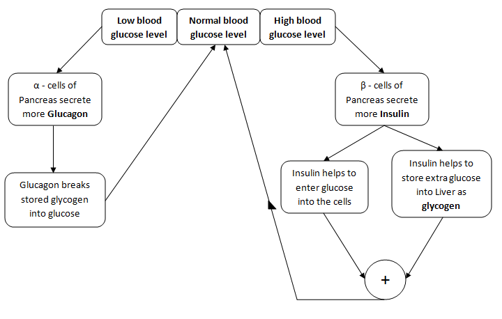
The human body needs to maintain homeostasis (dynamic equilibrium in human body) of blood glucose level. To maintain this homeostasis, mainly insulin and glucagon work together. Insulin is released from the -cells of pancreas, and glucagon is released from the -cells of pancreas. Figure 2 shows how human body maintains homeostasis with the help of these two hormones. When blood glucose level of the human body is higher than the normal level, the pancreas secretes more insulin. Insulin helps glucose to enter the cells. This also helps the extra glucose to get stored into the liver as glycogen, thus reducing the blood glucose level to maintain the homeostasis. However, when blood glucose level is low, the pancreas secretes glucagon which breaks stored glycogen into glucose and increases blood glucose level to normal level [4, 7, 11].
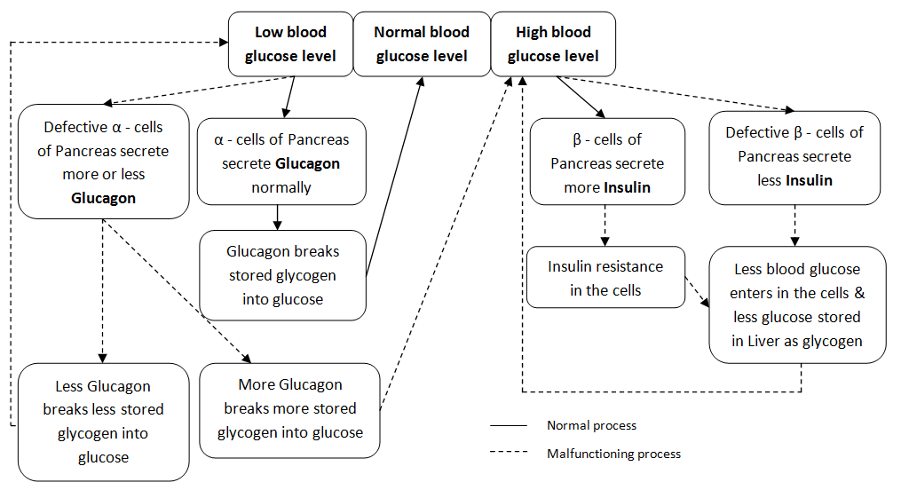
However for a diabetic person, the human body cannot maintain homeostasis of blood glucose level [Figure 3]. In type-1 diabetes, -cells of pancreas are destroyed by ones own immune system (T-cells). Thus less insulin is produced and for this insulin deficiency blood glucose level is high for a very long period.
In type-2 diabetes, cells of the human body becomes insulin resistant. So, insufficient amount of blood glucose enters into the cells. Also low amount of blood glucose gets stored into liver in the form of glycogen. To overcome this situation pancreas secretes excess insulin. If this excess insulin is enough to bring back blood glucose level to the normal level then the person is pre-diabetic. However if this excess insulin is not enough then the person is type-2 diabetic. Other reason for which blood glucose level can be high is due to malfunctioning -cells of pancreas. In this case they produce excess amount of glucagon [4, 6, 7].
3 Modeling glucose-insulin dynamics
In this section we first discuss a model suggested by previous authors. Next we go on to discuss the relevant factors that we have introduced into our model.
In 1964, E. Ackerman, J. W. Rosevear and W. F. McGuckin developed a mathematical model of Glucose-tolerance test [12]. In this model they have considered as blood-glucose concentration and as blood-insulin concentration. Here and were defined as fasting blood glucose level and fasting hormone (insulin) level respectively. and were defined as difference of the blood-glucose level and blood-hormone (insulin) level from the fasting levels respectively. So, and . The main equations used in that model are,
Where,
Rate constant of glucose removal independent of insulin.
Rate constant of glucose removal dependent of insulin.
Rate constant of insulin release due to glucose.
Rate constant of insulin removal independent of glucose.
= Rate of increase of blood glucose due to absorption of glucose from intestines.
We have modified the above model taking into account the contribution of the ingested glucose in the form of an additional differential equation. We explain this model using a block diagram where various parts of the human body represented by compartments. [Figure 4]

Let at time glucose disturbance of the digestive system (1st compartment) is . In this system we assume that the fasting glucose level is zero, thus glucose level and glucose disturbance is same. Let at time the blood (2nd compartment) glucose level is and the effective hormone level is . By the term effective hormone level means the net effect of all hormones (like insulin, glucagon) which can increase or decrease blood glucose level. The fasting blood glucose and the effective hormone levels and respectively. Let, and are the disturbances of the blood glucose level and the effective hormone level at time respectively. Thus we can write and . [12, 13]
In this model we make following assumptions :
- •
Rate of decrease in glucose disturbance in digestive system is proportional to its glucose disturbance () at time .
- •
Rate of increase in glucose disturbance in blood is proportional to the glucose which enters blood from digestive system () at time .
- •
Rate of hormone independent decrease of glucose disturbance in blood is proportional to its glucose disturbance () at time .
- •
Rate of hormone dependent decrease of glucose disturbance in blood is proportional to the effective hormone disturbance () at time .
- •
Rate of increase in effective hormone disturbance is proportional to the glucose disturbance in blood () at time .
- •
Rate of decrease in effective hormone disturbance is proportional to the effective hormone disturbance () at time .
Using these assumptions the model equations can be written as,
| (1) | |||||
| (2) | |||||
| (3) |
Time constant of decreasing glucose level in the digestive system, which is the total time to decrease glucose level to of the maximum value.
Rate constant of the hormone independent decrease of glucose level in the blood.
Rate constant of the hormone dependent decrease of glucose level in the blood.
Rate constant of release of the hormone due to blood glucose disturbance.
Rate constant for the removal of the hormone due to disturbance of the blood hormone level.
Amount of food that has been taken.
Percentage of glucose obtained in the body from the food that has been taken.
4 Stability analysis of this model
To determine fixed points we can write,
| Substituting in equation (1) we get, | ||||
| (4) | ||||
| Now making and and putting in equation (2) we get, | ||||
| (5) | ||||
| From equation (3) we get, | ||||
| (6) | ||||
| Solving equation (5), (6) we get, | ||||
| (7) | ||||
| and | ||||
| (8) | ||||
So the fixed point is . Thus equations can be written in the matrix form as,
Let,
Now characteristic equation is given by,
Here is the eigen values of matrix . So,
From this determinant we can write,
The above equation can write into two algebraic equations as, and .
Hence the first eigenvalue is where so and the other two eigenvalues are
If then . So, and are both negative.
If then is a complex quantity. Hence and are both complex with negative real part.
Hence the model is stable around .

Figure 5 represents a three dimensional phase portrait with different initial conditions. From this plots we can see that all the trajectories converge to the point (0,0,0). Hence (0,0,0) is a stable equilibrium point and the model is globally stable.
5 Calculation of glucose level in blood
In this section we obtain a solution for blood glucose level from the model equations by considering all initial conditions.
Solving equation we get,
| Where = Integrating constant. Substituting initial conditions, | ||||
| Hence, | ||||
| (9) | ||||
| Differentiating equation (2), | ||||
| (10) | ||||
| Substituting the relation of from equation (3) in equation (10) we get, | ||||
| After substituting relation of from equation (2) in equation (11) and rearranging we get, | ||||
| (11) | ||||
| Now using, , which is sum of the rate of hormone independent glucose removal and the hormone removal and we get, | ||||
| (12) | ||||
| Substituting from equation (9) we get, | ||||
| (13) | ||||
| Using | ||||
| (14) | ||||
| Solving equation (14), | ||||
| (15) | ||||
Where and and .
Now applying initial conditions and in equation we get,
So finally we get and .
So the disturbance in 2nd compartment is,
| (16) | ||||
| Hence glucose level in 2nd compartment is, | ||||
| (17) | ||||
From equation we can see that the solution of is like a oscillator with a small damping. can have both positive and negative values. Positive corresponds to the effective hormone level which decreases the blood glucose level. Similarly, negative corresponds to the effective hormone level which increases the blood glucose level. As we see, and can have many different values [12, 13]. So the crucial parameter turns out to be which in other words is a natural time period . If hours then the person is normal and if hours then the person is pre-diabetic [12, 13].
6 Modeling with experimental data
In this section, the blood glucose level that is obtained from our model is fitted with a data-set and essential parameters of our model are estimated. The data-set represents a glucose vs time data for a normal (Subject A) and a diabetic (Subject B) person. This data-set is taken from “Modeling Diabetes” by Joseph M. Mahaffy (Math 636 - Mathematical Modeling) [16].
| t in hour | Subject A | Subject B |
|---|---|---|
| 0 | 70 | 100 |
| 0.5 | 150 | 185 |
| 0.75 | 165 | 210 |
| 1 | 145 | 220 |
| 1.5 | 90 | 195 |
| 2 | 75 | 175 |
| 2.5 | 65 | 105 |
| 3 | 75 | 100 |
| 4 | 80 | 85 |
| 6 | 75 | 90 |

Figure 6 shows the best fit curve with confidence interval. confidence interval confidence interval is a statistically calculated interval from a observed data-set. This interval tells us that the true value of the parameter may be lie within it. Here, 1 confidence interval is defined as , =standard deviation of data and total number of data. If, increases then confidence interval decreases but confidence remains same.
The values of the obtained parameters are,
| Subject | in hour | ||||
|---|---|---|---|---|---|
| A | 73.8161 | 1.1733 | 2.4128 | 116.4327 | 0.6447 |
| B | 94.4838 | 0.8685 | 1.2823 | 208.3634 | 0.6242 |
| Subject | in hour | |||
|---|---|---|---|---|
| A | 1.1733 | 2.4128 | 2.6829 | 2.3418 |
| B | 0.8685 | 1.2823 | 1.5487 | 4.0569 |
= The fasting blood glucose level. It can vary person to person.
= Decay parameter of the damped oscillator.
= Angular frequency of damped oscillator.
From Table 2 we can see that value of both and for diabetic person is less than the normal person.
= Time constant of decreasing glucose level in the digestive system, which is the total time to decrease glucose level to of the maximum value. From Table 2 we can see that the value of this parameter is nearly equal for both normal and diabetic person.
= Natural angular frequency of damped oscillator.
= Natural time period of damped oscillator. From Table 3 we can see that value of for normal person is small than the diabetic person.
Here we plot the data-set and fit the function with 1 confidence interval [Figure 6]. Values of of Subject A and Subject B are 2.3418 hours and 4.0569 hours respectively [from Table 3], which indicates Subject A is normal and Subject B is mild diabetic. Thus it can be seen that the value of determines whether a person is pre-diabetic (for which hours) or not. This result nearly matches with the earlier model result but more accurate than the previous result to predict pre-diabetic condition. Also we found the value of a important parameter which is not included in the previous models. This parameter tells us how fast glucose enters in the blood from the digestive system. This parameter should be independent of the diabetes or blood glucose level at any time. From Table 2 we can see that the value of is nearly equal for both normal and diabetic person. So, is independent of diabetes and does not depend on blood glucose level.
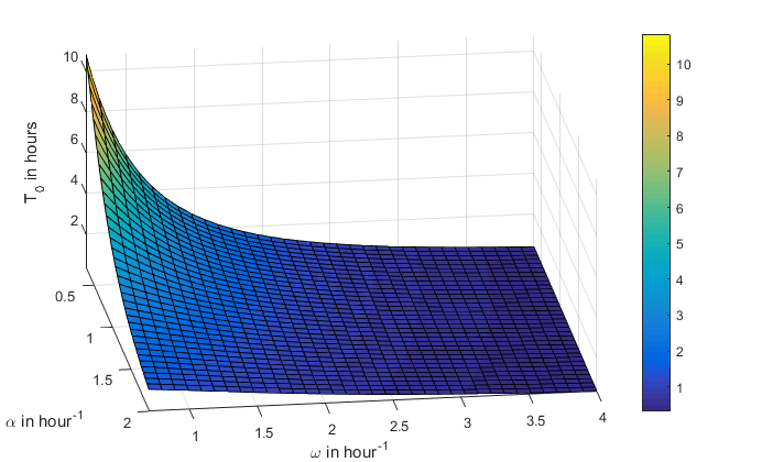

Figure 7 represents a three dimensional simulated surface plot which shows how varies with the possible range of and . We also see as and decreases, increases sharply after a point. High means that blood glucose level remains high for a long interval of time, which is the sign of a pre-diabetic case. Figure 8 represents a three dimensional simulated scatter plot. Here, blue dots represent normal cases (for which hours) and red dots represent pre-diabetic or diabetic (for which hours) cases. This plot shows that there exists two completely separate regions for normal and diabetic cases. It also shows that there is a large range of and which can vary person to person.
7 Discussion and Conclusion
In this paper, we have modified an existing model to a more realistic one by considering ingested glucose level, which is described by an additional ordinary differential equation. Here we have assumed that the externally ingested glucose decreases exponentially with time by increasing the blood glucose level, which is modeled by a parameter which describes how fast ingested glucose decreases. We have found that the model is globally stable around the fixed point (0,0,0). The solution imitates the behaviour of a damped harmonic oscillator and it converges to basal values normally observed in the human body. After fitting this relation to an available data-set, various fit parameters were obtained. Using these, the value of the parameter , which is the natural time period of a damped oscillator, was found. To conclude, we would like to point out that the most important improvement of this model over earlier models is it’s ability to predict the vulnerability of a person to be diabetic in the future. We have deduced that is less than 4 hours for a normal person and for a diabetic person, this time period is greater than 4 hours, which also matches the earlier established model predictions. Thus if a person has this natural time period of value around 4 hours, then it can be concluded that the person is susceptible to diabetes in future (pre-diabetic). However, in this model we consider that pancreas responded instantly with the blood glucose disturbance and hormone disturbance. But a small time delay of pancreatic response due to these disturbances will be more practical [32]. We can modify our model by considering this time delay. So, there is a lot of scope for further development of this model, which can enable precise and better control of this pre-diabetic stage and thus modify the quality of life of a human being.
Acknowledgment
We would like to thank Dr. Indrani Bose and Dr. Tanaya Bhattacharyya for their useful comments and suggestions. We also like to thank the Department of Physics, St. Xavier’s College for providing support during this work.
References
- [1] Reports of International Diabetes Federation (8th edition),2017.
- [2] Report of “Hindustan times”, World Diabetes Day: Number of Indians with diabetes likely to double in next decade, (Nov 14,2017 ).
- [3] Blood sugar regulation - Wikipedia.
- [4] The impact of mathematical modeling on the understanding of diabetes and related complications : I Ajmera, M Swat, C Laibe, N Le Novère and V Chelliah, CPT: Pharmacometrics & Systems Pharmacology (2013) 2, e54; doi:10.1038/psp.2013.30.
- [5] Diabetes fact sheet - WHO (15 November 2017).
- [6] Diabetes mellitus - Wikipedia.
- [7] Classification and Diagnosis of Diabetes Diabetes Care 2015; American Diabetes Association; 38(Suppl. 1):S8–S16 | DOI: 10.2337/dc15-S005.
- [8] Diabetes model of care , Endocrine Health Network, 2008.
- [9] Experimental Models on Diabetes: A Comprehensive Review By Radha Sharma, Vivek Dave, Swapnil Sharma, Pankaj Jain, Sachdev Yadav, International Journal of Advances in Pharmaceutical Sciences 4 (2013) 01-08.
- [10] Cellular respiration- Wikipedia.
- [11] Automatic Blood Glucose Control in Diabetes, Marit Owren, Norwegian University of Science and Technology Department of Engineering Cybernetics.
- [12] A Mathematical Model of the Glucose-tolerance test, Eugene Ackerman, John W. Rosevear, Warren F. McGuckin, Phys. Med. Biol. 1964, Vol. 9, No. 2, 203-213.
- [13] Tests of a Mathematical Model of the Blood-Glucose Regulatory System, LC. Gatewood, Eugene Ackerman, John W. Rosevear, and George D. Molnar, COMPUTERS AND BIOMEDICAL RESEARCH 2, 1-14 (1968).
- [14] Model studies of blood-glucose regulation, Eugene Ackerman, LC. Gatewood, John W. Rosevear, and George D. Molnar, Bull Math Biophys, 27, suppl: 21-suppl: 37.
- [15] Modelling Blood Glucose Dynamics, LC. Gatewood, Eugene Ackerman, John W. Rosevear, and George D. Molnar, Behavioral Science, Volume 15, 197.
- [16] Modeling Diabetes By Joseph M. Mahaffy, Math 636, Fall 2017.
- [17] Nonlinear Dynamics and Chaos, Steven H. Strogatz, 2nd ed.
- [18] A Mathematical Model of Glucose - Insulin regulation under the influence of externally ingested glucose (G-I-E model), Anuradha Devi, Ranjan Kalita, Aditya Ghosh, International Journal of Mathematics and Statistics Invention (IJMSI) Volume 4 Issue 5 || June. 2016 || PP-54-58.
- [19] An interactive Glucose- Insulin regulation under the influence of Externally Ingested Glucose model, Anuradha Devi, Ranjan Kalita, Aditya Ghosh, Global Journal of Mathematical Sciences: Theory and Practical. ISSN 0974-3200 Volume 9, Number 3 (2017), pp. 277-285.
- [20] Mathematical Model for Detecting Diabetes in the Blood, B. Kwach, O. Ongati, R. Simwa, Applied Mathematical Sciences, Vol. 5, 2011, no. 6, 279 - 286.
- [21] Modeling and Simulation of Glucose-Insulin Dynamics, Allan Lyngby Lassen, Thor Schtt Svane Nielsen, Kongens Lyngby 2008 IMM-B.Sc.-2008-18.
- [22] Closed loop blood glucose control in diabetics, Faiz-Ul-Hassan, Muhammad Adil, Ali Khaqan, Sana Shuja, Moazzam Islam Tiwana, Qadeer-ul- Hassan, Shahzad Malik, Raja Ali Riaz, Biomedical Research 2017; 28 (16): 7230-7236.
- [23] Quantitative estimation of insulin sensitivity By Richard N. Bergman, Y. Ziya Ider, Charles R. Bowden , and Claudio Cobelli , Am J Biophysics, 236, E667-E677,(1979).
- [24] Mathematical Model for Glucose-Insulin Regulatory System of Diabetes Mellitus, Sandhya and Deepak Kumar, Advances in Applied Mathematical Biosciences. ISSN 2248-9983 Volume 2, Number 1 (2011), pp. 39-46.
- [25] A mathematical model of glucose-insulin interaction, Jamal Hussain and Denghmingliani Zadeng, Science vision, 14(2), 84-88.,(2014).
- [26] Minimal Models for Glucose and Insulin Kinetics - A Matlab implementation, NATAL VAN RIEL , version of February 5, 2004, DOI: 10.13140/2.1.1766.7361.
- [27] MINMOD: a computer program to calculate insulin sensitivity and pancreatic responsivity from the frequently sampled intravenous glucose tolerance test, Giovanni Pacini and Richard N. Bergman, Computer Methods and Programs in Biomedicine 23 (1986) 113-122.
- [28] A critical review of mathematical models and data used in diabetology, A Boutayeb and A Chetouani, BioMedical Engineering OnLine 2006, 5:43 doi:10.1186/1475-925X-5-43.
- [29] Mathematical Biology I. An Introduction, Third Edition, By J.D. Murray.
- [30] Use of Glycated Haemoglobin (HbA1c) in the Diagnosis of Diabetes Mellitus, Abbreviated Report of a WHO Consultation.
- [31] Hemoglobin A1c (HbA1c) Test for Diabetes(Article), www.webmd.com.
- [32] A Mathematical Model of Glucose-Insulin Interaction with Time Delay, Saber S, Bashier EBM , Alzahrani SM and Noaman IA, Journal of Applied & Computational Mathematics (2018), DOI: 10.4172/2168-9679.1000416.