A comparison of maximum likelihood and absolute moments
for the estimation of Hurst exponents
in a stationary framework

If $X$ is an fBm of parameters $H$ and $\sigma^{2}$, it has the property of $H$-self-similarity: whatever $c>0$ and $\tau\geq 0$, $X_{\tau}\overset{d}{=}c^{-H}X_{c\tau}$, where $\overset{d}{=}$ means equality in finite-dimensional distributions. Since $X_{0}=0$, we also have $X_{\tau}-X_{0}\overset{d}{=}c^{-H}(X_{c\tau}-X_{0})$. By stationarity of the increments of the fBm $X$, whatever $s>0$, we have $X_{s+\tau}-X_{s}\overset{d}{=}X_{\tau}-X_{0}\overset{d}{=}\tau^{H}X_{1}$. In particular, this increment has a variance equal to $\tau^{2H}\sigma^{2}$. We can use this property to estimate $H$. Indeed, the empirical variance of the increments of duration $\tau$, $M_{\tau}(X)$, is a sum of identically distributed terms, and it converges towards $\tau^{2H}\sigma^{2}$. The basic absolute-moment estimation thus consists in identifying the slope, expectedly equal to $2H$, of the log-log plot $\ln(\tau)\mapsto\ln(M_{\tau}(X))$ [14].

We can replace the variance $M_{\tau}$ by an empirical absolute moment of another order [14]. More generally, we can define an absolute moment of order $k>0$ for any process $S$ observed between times $t_{a}$ and $t_{b}$, with $N$ equispaced increments of duration $\tau=(t_{b}-t_{a})/N$:

The estimator of $H$ is then $-1/k$ times the slope of the log-log plot $\ln(N)\mapsto\ln(M_{k,N,t_{a},t_{b}}(S))$.

We now observe a stationary process, $Y$. By Lamperti Theorem, it is the inverse Lamperti transform of parameters $H$ and $\theta$ of an $H$-self-similar process, $X$ [16]. We also assume that $X$ is an fBm of Hurst exponent $H$. As the absolute-moment method is designed for the fBm, it is not the proper tool to estimate $H$ directly on $Y$ [18]. So, it sounds better to transform $Y$ first in a self-similar process $Z$, thanks to a direct Lamperti transform of parameters $H^{\prime}$ and $\theta^{\prime}$, and to estimate $H$ by applying the absolute-moment method on $Z$. We should preferably choose $H^{\prime}=H$ and $\theta^{\prime}=\theta$, so that $Z$ is equal to $X$ and is therefore an fBm, for which the absolute-moment method is relevant. But $H$ is unknown in practice and we cannot use it to transform $Y$ in $Z=X$. As a consequence, $Z$ is not necessarily an fBm, although it is $H^{\prime}$-self-similar [16]. As exposed by the following theorem, increments of $Z$ are not stationary in general. It means that $M_{k,N,t_{a},t_{b}}(Z)$ is not a sum of identically distributed terms, and that the log-log plot provides us with a slope which is not $-kH^{\prime}$ in general. The log-log plot has even an asymptote of slope $-kH$ for $N\rightarrow+\infty$. These properties, exposed in Theorem 1, are pivotal for building the AAM estimation method.

The proof of Theorem 1 is postponed in Appendix A.

In addition, with the assumptions of Theorem 1, $Z$ is $H^{\prime}$-self-similar, while $X$ is $H$-self-similar and $Y$ is not self-similar but stationary [16]. The particular case $(H^{\prime},\theta^{\prime})=(H,\theta)$ is of interest, as it is the only case for which the log-log plot of $Z$ is indeed affine of slope $-kH^{\prime}$, as we will see in Theorem 2. The AAM method presented in the next paragraph capitalizes on this property.

The absolute-moment method is widespread and efficient for estimating Hurst exponents in the case of self-similar processes. We want to adapt this method to the case of a stationary process. To do so, we transform the stationary process in a self-similar one thanks to the direct Lamperti transform. We can then apply the basic absolute-moment method to this transformed process. However, this simple idea raises two difficulties: one is about the choice of the parameters in the Lamperti transform, the other on the estimation of the moments. For simplicity, we now focus on second-order moments.

Regarding the first issue, in order to transform the stationary process $Y$ into a self-similar one, we need to choose a scaling parameter $H^{\prime}$ and a time change parameter $\theta^{\prime}$. We restrict the framework by assuming that the stationary process is itself the inverse Lamperti transform of an fBm with unknown parameters $H$ and $\theta$. We will show in Theorem 2 that one and only one choice for the pair $(H^{\prime},\theta^{\prime})$ can lead to an fBm of Hurst exponent $H^{\prime}$: it is precisely $(H,\theta)$. As a consequence, we are going to select the pair $(H^{\prime},\theta^{\prime})$ so that $Z=\mathcal{L}_{H^{\prime},\theta^{\prime}}Y$ is revealed to be an fBm of Hurst exponent $H^{\prime}$. The absolute-moment method makes it possible to check if we meet this property. Indeed, if the process is an fBm, the log-log plot must be affine, and if its Hurst exponent is $H^{\prime}$, the slope of the log-log plot must be $2H^{\prime}$. We thus propose an iterative optimization procedure, using Nelder-Mead algorithm as for the ML method. The purpose of this procedure is to find the pair $(H^{\prime},\theta^{\prime})$ minimizing the objective function $f_{\mathcal{S}}(H^{\prime},\theta^{\prime})=|\hat{H}_{H^{\prime},\theta^{\prime}}-H^{\prime}|+|\hat{\alpha}_{H^{\prime},\theta^{\prime}}-1|$, where $\hat{H}_{H^{\prime},\theta^{\prime}}$ and $\hat{\alpha}_{H^{\prime},\theta^{\prime}}$ are respectively half the slope and a linearity parameter of the log-log plot of $\mathcal{L}_{H^{\prime},\theta^{\prime}}Y$ on a set of scales $\mathcal{S}$. More specifically, if $M_{H^{\prime},\theta^{\prime},\tau}$ is the moment¹¹ 1 If $(H^{\prime},\theta^{\prime})\neq(H,\theta)$, the increments of the process are not stationary according to Theorem 1. So the word moment is improper for these increments. For concision, we however keep this word to designate the average of moments of increments at various times. of the increments of $\mathcal{L}_{H^{\prime},\theta^{\prime}}Y$ of duration $\tau$, we obtain $\hat{H}_{H^{\prime},\theta^{\prime}}$ and $\hat{\alpha}_{H^{\prime},\theta^{\prime}}$ by the following regression: $\ln\left(M_{H^{\prime},\theta^{\prime},\tau}\right)=\ln\left(M_{H^{\prime},\theta^{\prime},\tau_{min}}\right)+2\hat{H}_{H^{\prime},\theta^{\prime}}(\ln(\tau)-\ln(\tau_{min}))^{\hat{\alpha}_{H^{\prime},\theta^{\prime}}}$, where $\tau_{min}$ is the smallest time step observed in the log-log plot and $\tau\in\mathcal{S}$. Theoretically, this regression leads to $\hat{H}_{H^{\prime},\theta^{\prime}}=H^{\prime}$ and $\hat{\alpha}_{H^{\prime},\theta^{\prime}}=1$ only for $(H^{\prime},\theta^{\prime})=(H,\theta)$, as stated in the following theorem, which justifies the relevance of the proposed estimation method.

The proof of Theorem 2 is postponed in Appendix B.

The other challenge in the stationary adaptation of the absolute-moment method is about estimating properly moments of increments of the transformed process $\mathcal{L}_{H^{\prime},\theta^{\prime}}Y$. This transformation indeed distorts the times. We now observe the process at irregularly sampled dates. The ML method can nicely face this irregular sampling [23]. But the estimation of absolute moments is not as straightforward. In the current work, we have implemented a semi-parametric estimation of the absolute moments. We have used a kernel regression on the absolute increments of the observed process with a fractal correction of their scale. For estimating the absolute moment of increments of duration $\tau$, we have indeed taken into account various absolute increments of duration $d$ close to $\tau$, which we have multiplied by $(\tau/d)^{2H^{\prime}}$.

We now introduce pseudo-codes which expose how the AAM method is to be implemented. We divide the estimation procedure in two steps. The first one is about optimizing the parameters $H$ and $\theta$ and the second one about the implementation of the objective function to be optimized. The first step is not very specific and is shared by the two approaches. Indeed, in the ML approach, instead of minimizing the objective function implemented in Algorithm 2, one uses Algorithm 1 to maximize the log-likelihood detailed in equation (2).

The optimization engine in Algorithm 1 is quite simple to use and can be applied to both estimation methods. Nevertheless, this algorithm may be improved. First, the parameters $H$ and $\theta$ are constrained to remain in the intervals $(0,1)$ and $(0,+\infty)$. In a basic version of Nelder-Mead, we can simply force the parameters to be in these intervals, by changing forbidden values by one close to the border, following Box’s method [6]. Alternative promising solutions for dealing with constraints include a random version of Box’s method as well as a transform such as $x\in\mathbb{R}\mapsto\frac{1}{2}+\frac{1}{\pi}\arctan(x)\in(0,1)$ for $H$ and $x\in\mathbb{R}\mapsto\exp(x)\in(0,+\infty)$ for $\theta$ [27].

In Algorithm 1, the initialization of the simplex relies on some arbitrary values which are not too close in order not to stop prematurely the algorithm, and not too distant from each other in order not to cross the bounds after the first iteration. The values displayed for the initialization in Algorithm 1 are only indicative. Other reasonable deterministic or random initializations lead to similar results. We could also call three times this optimizer with three distinct initializations and then use these three solutions as the initialization of a last Nelder-Mead optimization.

The stopping criterion

is intended to depict the situation in which the vertices of the simplex are close enough to consider that a local optimum has been found. A criterion on the number of iterations may also be introduced.

The objective function in Algorithm 1 is quite simple in the ML case since it is related to the log-likelihood. The most time-consuming part for computing this likelihood is the inversion of the symmetric definite-positive matrix $\Sigma$. The objective function in the AAM approach is based on the analysis of the log-log plot of the Lamperti transform of the data. It is exposed in Algorithm 2, which is the main methodological contribution of this paper.

We note that, in Algorithm 2, we have simplified the two-dimensional regression leading to $\hat{H}_{H^{\prime},\theta^{\prime}}$ and $\hat{\alpha}_{H^{\prime},\theta^{\prime}}$ by two one-dimensional regressions. If $(H,\theta)=(H^{\prime},\theta^{\prime})$, the two regressions should lead to $\hat{H}=H^{\prime}$ and $\hat{\alpha}=1$. This justifies the relevance of the simplification.

In the simulation study, we have considered equally-spaced observation times with a time step $h=t_{i+1}-t_{i}=0.001$. In the study presented in Section 4, the set of scales $\mathcal{S}$, gathered in Algorithm 2 in the vector R, is such that the smallest scale considered is $\tau_{\min}=\textbf{R}[1]=\ln(e^{\theta h}-1)$ and the biggest $\textbf{R}[n]=\ln(e^{\theta h\rho N}-1)$, where $\rho\in(0,1)$ is a meta-parameter linking this biggest step to a proportion $\rho$ of the whole duration $Nh$ of the signal. Other scales in $\mathcal{S}$ simply make a regular sampling of the interval $[\tau_{\min},\textbf{R}[n]]$.

The kernel $K$ used in the semi-parametric approximation of the moments does not play a decisive role in the results, according to the simulations we made. For decreasing the computational time, it is better to consider a kernel with bounded support, such as Epanechnikov or a truncated Gaussian. In this case, the choice of the bandwidth parameter of the kernel is to be made so that the total weight $W$, appearing in Algorithm 2 and corresponding to the scales selected in $\mathcal{S}$, is never equal to zero.

We compare the ML and the AAM methods for estimating the parameters $H$ and $\theta$ of simulated delampertized fBms, with a Hurst exponent 0.65 and a time change parameter equal to 30. The functions that we optimize, either with a max for the likelihood or with a min for the objective function of the AAM method, are quite smooth curves, as one can see in Figure 1. This eases the optimization. However, we see in Figure 2 that local minima may appear in the estimation of $\theta$ in the AAM approach. A more sophisticated algorithm, such as a genetic algorithm, instead of the Nelder-Mead algorithm, could probably increase the accuracy of the method. As already evoked, many pairs $(H,\theta)$ have a close likelihood, as a ridge with very high likelihoods appears in Figure 1. This can make also the estimation in the ML approach unstable.

The average estimated parameters are close to the true parameters for both the ML and the AAM methods, as reported in Table 1. The uncertainty in the estimation, revealed by the standard deviation, is higher for the ML with respect to $\theta$, and higher for the absolute moments with respect to $H$.

We now study by simulations the impact of the input parameters and of methodological choices.

First, regarding the estimation of $\theta$ the ML method is undoubtedly more accurate than the AAM method, whatever the size of the sample. For example, for 100 simulated time series of length 200, with $H=0.65$, we obtain a standard deviation of the estimated $\theta$ very close to the average in the AAM case, whereas with ML the standard deviation is lower and the average closer to the actual value of $\theta$, as one can see in Table 2. We also note that reducing the sample size from 200 to 50 approximatively doubles the standard deviation of both the ML and AAM estimators.

The results regarding the estimation of $H$ are still slightly in favour of the ML method as soon as the sample size is small, but the difference between the two methods is more restricted in particular for greater values of $H$, as one can see in Table 3. The real benefit of using the AAM method appears for greater sample sizes, for which the ML method is almost unusable due to unreasonably long execution time, as reported in Table 4. For the AAM approach, we get, in a limited time, results which have roughly the same accuracy as estimates obtained for shorter time series, as exposed in Table 5.

The execution time displayed for the AAM method in Table 4 in fact depends on some methodological choices, in particular the regression design. For instance, simulations show that the execution time depends linearly on the number $n$ of moments considered in the regression. This is consistent with the intuition. In Table 4, we have chosen $n=15$. However, beyond the execution time, the accuracy of the AAM method, both in terms of bias and variance, does not seem to be affected by $n$, according to simulations, at least for the values we have tested, between $n=15$ and $n=150$. The choice of the kernel and refinements on the choice of the bandwidth do neither seem to affect the accuracy.

We now show how the AAM framework makes it possible to determine whether the model is well specified or not. We known that the ML approach fails in this task, since it simply outputs parameters maximizing a likelihood, even when the model is not relevant. We can improve the ML approach by considering a set of various (fractal and stationary) models and ratios of likelihood or information criteria [5]. This will in fact only help finding the best model in a predefined family of models but not clearly state the good specification of the selected model.

We work with simulated data generated by two distinct models:

•    $\triangleright$

  Time series 1 follows the specification mentioned above: it is a delampertized fBm of Hurst exponent $H=0.5$, variance 1, and time change parameter $\theta=30$. For this particular choice of Hurst exponent, the delampertized fBm is equivalent to an Ornstein-Uhlenbeck process.

•    $\triangleright$

  Time series 2 is the sum of two processes: a delampertized fBm with the same parameters as Time series 1, and a Gaussian noise process of standard deviation $40\%$.

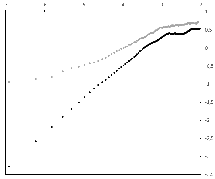
We display the two trajectories of these processes in Figure 3, as well as their corresponding log-log plot. For Time series 1, we observe a flattening of the curve at higher scales, which corresponds to the stationary feature. For Time series 2, in addition to the same flattening at high scales, we observe a second one at small scales. This is a well-known effect of additive noise on the log-log plot [26].

We then use the ML approach to estimate the parameters. The likelihood used follows equation 2 and corresponds to a delampertized fBm. We thus expect this method to provide satisfying results for Time series 1 but not for Time series 2, since another specification is required. Table 6 confirms this intuition with poor results for Time series 2, for instance a Hurst exponent equal to 0.267 very far from the true and unobserved value (0.5). However, when estimating the parameters with the ML method, we have no clue that the model and therefore the estimation are flawed. The estimated parameters are simply the best, provided that the model is well specified.

In order to check that the model is well specified, one can use the tools introduced for the AAM approach. More precisely, using the parameters $H^{\prime}$ and $\theta^{\prime}$ estimated with the ML method, one can Lamperti-transform the time series and consider the log-log plot of the transformed series, as displayed in Figure 4. If the model is well specified, the log-log plot of the transformed series should be the one of an fBm, that is linear. For Time series 1, the log-log plot is indeed linear. Visually, we thus cannot assess that the delampertized fBm is not well specified for this time series. Regarding the transformed version of Time series 2, the aspect of the log-log plot is not really the one expected if the delampertized fBm was an appropriate choice of model, in particular because the curve stops growing for higher scales.

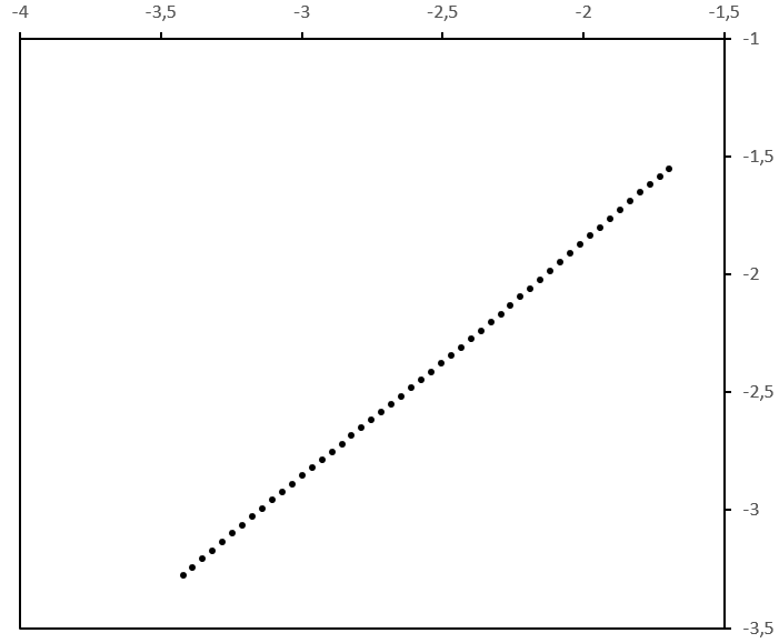
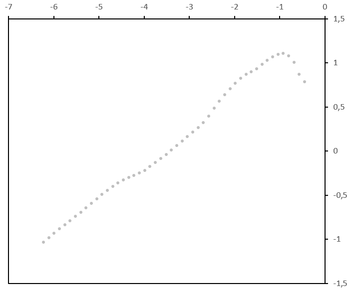
More quantitatively than visually, according to Theorem 2, in case of good specification, the log-log plot of the transformed series should be linear with a slope equal to $2\times H^{\prime}$. In this case, we thus should have $\hat{H}_{H^{\prime},\theta^{\prime}}$ close to $H^{\prime}$ and $\hat{\alpha}_{H^{\prime},\theta^{\prime}}$ close to 1, where the metric $\hat{H}_{H^{\prime},\theta^{\prime}}$ is the half slope and $\hat{\alpha}_{H^{\prime},\theta^{\prime}}$ the linearity indicator introduced in Section 3.3. We see in Table 6 that the linearity indicators of the two log-log plots are roughly equally close to 1. More interestingly, the quantity $\hat{H}_{H^{\prime},\theta^{\prime}}-H^{\prime}$ is close to 0 (exactly 0.002) for Time series 1 and 36 times higher (0.072) for Time series 2. This undoubtedly confirms that a delampertized fBm is not an appropriate model for Time series 2.

References

- [1] A. Ammy-Driss and M. Garcin. Efficiency of the financial markets during the COVID-19 crisis: time-varying parameters of fractional stable dynamics. arXiv preprint, 2020.
- [2] A. Andresen, F.E. Benth, S. Koekebakker, and V. Zakamulin. The CARMA interest rate model. International journal of theoretical and applied finance, 17(2):1450008, 2014.
- [3] M. Bennedsen, A. Lunde, and M.S. Pakkanen. Decoupling the short-and long-term behavior of stochastic volatility. Journal of financial econometrics, page nbaa049, 2021.
- [4] S. Bianchi. Pathwise identification of the memory function of multifractional Brownian motion with application to finance. International journal of theoretical and applied finance, 8(2):255–281, 2005.
- [5] S. Bianchi and Q. Li. A new estimator of the self-similarity exponent through the empirical likelihood ratio test. Journal of statistical computation and simulation, 90(11):1982–2001, 2020.
- [6] M.J. Box. A new method of constrained optimization and a comparison with other methods. Computer journal, 8(1):42–52, 1965.
- [7] D.C. Brody, J. Syroka, and M. Zervos. Dynamical pricing of weather derivatives. Quantitative finance, 2(3):189–198, 2002.
- [8] A. Brouste and S.M. Iacus. Parameter estimation for the discretely observed fractional Ornstein-Uhlenbeck process and the Yuima R package. Computational statistics, 28(4):1529–1547, 2013.
- [9] P. Cheridito, H. Kawaguchi, and M. Maejima. Fractional Ornstein-Uhlenbeck processes. Electronic journal of probability, 8(3):1–14, 2003.
- [10] Y.W. Cheung, D.C. Tam, and M.S. Yiu. Does the Chinese interest rate follow the US interest rate? International journal of finance & economics, 13(1):53–67, 2008.
- [11] L. Chevillard. Regularized fractional Ornstein-Uhlenbeck processes and their relevance to the modeling of fluid turbulence. Physical review E, 96(3):033111, 2017.
- [12] A. Chronopoulou and F.G. Viens. Estimation and pricing under long-memory stochastic volatility. Annals of finance, 8(2-3):379–403, 2012.
- [13] J.-F. Coeurjolly. Estimating the parameters of a fractional Brownian motion by discrete variations of its sample paths. Statistical inference for stochastic processes, 4(2):199–227, 2001.
- [14] J.-F. Coeurjolly. Identification of multifractional Brownian motion. Bernoulli, 11(6):987–1008, 2005.
- [15] J.F. Diaz and J.H. Chen. Testing for long-memory and chaos in the returns of currency exchange-traded notes (ETNs). Journal of applied finance and banking, 7(4):15–37, 2017.
- [16] P. Flandrin, P. Borgnat, and P.-O. Amblard. From stationarity to self-similarity, and back: Variations on the Lamperti transformation. In Processes with long-range correlations, pages 88–117. Springer, Berlin-Heidelberg, 2003.
- [17] M. Garcin. Estimation of time-dependent Hurst exponents with variational smoothing and application to forecasting foreign exchange rates. Physica A: statistical mechanics and its applications, 483:462–479, 2017.
- [18] M. Garcin. Hurst exponents and delampertized fractional Brownian motions. International journal of theoretical and applied finance, 22(5):1–26, 2019.
- [19] M. Garcin. Fractal analysis of the multifractality of foreign exchange rates. Mathematical methods in economics and finance, 13-14(1):49–73, 2020.
- [20] M. Garcin. Forecasting with fractional Brownian motion: a financial perspective. arXiv preprint, 2021.
- [21] M. Garcin and M. Grasselli. Long versus short time scales: the rough dilemma and beyond. to appear in Decisions in economics and finance, 2020.
- [22] J. Gatheral, T. Jaisson, and M. Rosenbaum. Volatility is rough. Quantitative finance, 18(6):933–949, 2018.
- [23] S. Hidot, C. Saint-Jean, and J.-Y. Lafaye. Etude expérimentale de l’influence d’un échantillonnage irrégulier dans l’estimation du paramètre de Hurst. Journal de la société française de statistique, 149(1):81–95, 2008.
- [24] Y. Hu and D. Nualart. Parameter estimation for fractional Ornstein-Uhlenbeck processes. Statistics & probability letters, 80(11-12):1030–1038, 2010.
- [25] J. Lamperti. Semi-stable stochastic processes. Transactions of the American mathematical society, 104(1):62–78, 1962.
- [26] Y. Lanoiselée, G. Sikora, A. Grzesiek, D.S. Grebenkov, and A. Wyłomańska. Optimal parameters for anomalous-diffusion-exponent estimation from noisy data. Physical review E, 98(6):062139, 2018.
- [27] F. Le Floc’h. Issues of Nelder-Mead simplex optimisation with constraints. SSRN eLibrary, page 2097904, 2012.
- [28] B. Mandelbrot and J. van Ness. Fractional Brownian motions, fractional noises and applications. SIAM review, 10(4):422–437, 1968.
- [29] J. Mielniczuk and P. Wojdyłło. Estimation of Hurst exponent revisited. Computational statistics & data analysis, 51(9):4510–4525, 2007.
- [30] S.K. Mitra. Is Hurst exponent value useful in forecasting financial time series? Asian social science, 8(8):111–120, 2012.
- [31] M. Mossberg and E. Mossberg. A note on parameter estimation in Lamperti transformed fractional Ornstein-Uhlenbeck processes. IFAC proceedings volumes, 45(16):1067–1072, 2012.
- [32] P.K. Narayan and S.S. Sharma. Does data frequency matter for the impact of forward premium on spot exchange rate? International review of financial analysis, 39:45–53, 2015.
- [33] J.A. Nelder and R. Mead. A simplex method for function minimization. Computer journal, 7(4):308–313, 1965.
- [34] C.J. Nuzman and H.V. Poor. Linear estimation of self-similar processes via Lamperti’s transformation. Journal of applied probability, 37(2):429–452, 2000.
- [35] R.F. Peltier and J. Lévy Véhel. A new method for estimating the parameter of fractional Brownian motion. Technical report 2396, INRIA, 1994.
- [36] W. Robbertse and F. Lombard. On maximum likelihood estimation of the long-memory parameter in fractional Gaussian noise. Journal of statistical computation and simulation, 84(4):902–915, 2014.
- [37] L. Shi. Does security transaction volume-price behavior resemble a probability wave? Physica A: statistical mechanics and its applications, 366:419–436, 2006.
- [38] T. Simos and M. Tsionas. Bayesian inference of the fractional Ornstein-Uhlenbeck process under a flow sampling scheme. Computational statistics, 33(4):1687–1713, 2018.
- [39] L. Viitasaari. Representation of stationary and stationary increment processes via Langevin equation and self-similar processes. Statistics & probability letters, 115:45–53, 2016.
- [40] M. Šapina, M. Garcin, K. Kramarić, K. Milas, D. Brdarić, and M. Pirić. The Hurst exponent of heart rate variability in neonatal stress, based on a mean-reverting fractional Lévy stable motion. Fluctuation and noise letters, 19(3):2050026, 2020.
Appendix A Proof of Theorem 1
Proof.
The results concerning and are standard properties [16, 18]. Let us now focus on the process .
-
First, we note that, whatever ,
(6) where we introduced . This process is extended by . We obtain this extension trivially if , and using equation (6) else: .
This variance of the increments varies with . We prove this property by considering the asymptotic behaviour of the variance, for . Indeed, we have, using equation (7) together with asymptotic expansions and the fact that :
(8) This asymptote depends on , as soon as , so increments are not stationary in this case. If , we cannot conclude that increments are stationary and we must go further in our stationarity analysis. We thus consider the variance of increments with a given , for :
(9) and for , that is for , using equation (8) with :
(10) The two variances, when , are equal only if . We thus have the necessary condition: stationarity of increments is only possible when both and .
The sufficient condition is straightforward. Indeed, when and , then and equation (7) gives exactly, , , which does not depend on .
∎
Appendix B Proof of Theorem 2
We prove first the sufficient condition. If , then , for all , and the statement is trivial.
Regarding the necessary condition, if we assume that reaches the theoretical minimum of , which is zero according to the particular case , then and . As we have the same and whatever , we conclude that the plot is affine. Regarding the slope, after equation (8), it is for small scales, but also for all scales because the log-log plot is affine, so that . The value of which minimizes is thus . If we follow the notation of Theorem 1, with , we should have , that is, following equations (4) and (5),
which is true only if . Therefore . ∎