Overhead-Aware Design of Reconfigurable Intelligent Surfaces in Smart Radio Environments
Abstract
Reconfigurable intelligent surfaces have emerged as a promising technology for future wireless networks. Given that a large number of reflecting elements is typically used and that the surface has no signal processing capabilities, a major challenge is to cope with the overhead that is required to estimate the channel state information and to report the optimized phase shifts to the surface. This issue has not been addressed by previous works, which do not explicitly consider the overhead during the resource allocation phase. This work aims at filling this gap, by developing an overhead-aware resource allocation framework for wireless networks where reconfigurable intelligent surfaces are used to improve the communication performance. An overhead model is proposed and incorporated in the expressions of the system rate and energy efficiency, which are then optimized with respect to the phase shifts of the reconfigurable intelligent surface, the transmit and receive filters, the power and bandwidth used for the communication and feedback phases. The bi-objective maximization of the rate and energy efficiency is investigated, too. The proposed framework characterizes the trade-off between optimized radio resource allocation policies and the related overhead in networks with reconfigurable intelligent surfaces.
I Introduction
Future wireless networks will be a pervasive platform, which will not only connect us but will embrace us through a plethora of services. The ubiquity, speed, and low latency of such networks will allow currently disparate devices and systems to become a distributed intelligent communications, sensing, and computing platform [1]. Small-cell networks [2], massive multiple-input-multiple-output systems [3], and millimeter-wave communications [4] are three fundamental technologies that will spearhead the emergence of future wireless networks [5]. The question is, however, whether these technologies will be sufficient to meet the requirements of future networks that integrate communications, sensing, and computing in a single platform. Wireless networks, in addition, are evolving towards a software-defined paradigm, where every part of the network can be configured and controlled via software [6], [7]. However, the wireless environment, i.e., the channel, is generally uncontrollable, and often an impediment to be reckoned with, e.g. signal attenuation limits network connectivity, multi-path propagation results in fading, reflections from objects produce uncontrollable interference.
Motivated by these considerations, the concept of “smart radio environment” has recently emerged [8, 9, 10, 11], wherein the environmental objects are envisioned to be coated with man-made intelligent surfaces of configurable electromagnetic materials that are referred to as reconfigurable intelligent surfaces (RISs) [12], [13]. These materials are expected to contain integrated electronic circuits and software that will enable them to control the wireless medium [10], [14]. Conceptually, an RIS can be viewed as a reconfigurable mirror or lens, depending on its configuration [15], that is made of a number of elementary elements, often referred to as meta-atoms or passive scatterers, that are configurable and programmable in software. The input-output response of each passive scatterer can be appropriately customized, so that the signals impinging upon the RIS can be predominantly reflected or transmitted in specified directions or focused towards specified locations [16], [17]. RISs have the potential to enable the control of the propagation environment, thus potentially changing the design of wireless networks.
Due to the potential opportunities offered by RIS-empowered wireless networks, a large body of research contributions have recently appeared in the literature. The interested readers are referred to the survey papers in [10, 18, 19, 20, 21], where a comprehensive description of the state-of-the-art, the scientific challenges, the distinctive differences with other technologies, and the open research issues are comprehensively discussed. In [22], systems made of large active surfaces are put forth as the natural evolution of massive MIMO systems. A similar idea is embraced in [23], where it is elaborated on how RISs can be used to implement massive MIMO systems, replacing each conventional antenna with an active reconfigurable surface. The fundamental performance of the system is analyzed, showing that it grants satisfactory performance, while at the same time reducing costs, power consumption, and physical size. In [24] it is shown how RISs can yield better performance compared to the use of relays. Moreover, in [25] it is shown that RISs can improve the secrecy of communication by focusing the transmit signal only towards the direction of the intended receivers. Recently, in addition, a few experimental testbeds have been built to substantiate the feasibility of RISs, e.g., [26], [27], [28, 29, 30]. In the following two sub-sections, we describe the contributions that are most related to the present paper, and outline novelty and contributions of our work.
I-A Related Works
We focus our attention on the issue of resource allocation in RIS-empowered wireless networks. In this context, several research papers have appeared recently, mostly considering application scenarios where the line-of-sight link is either too weak or is not available, and, therefore, an RIS is employed to enable the communication through the optimization of the phase shifts of its individual passive elements and of the precoding and decoding vectors of the transmitter and receiver, respectively. In [31], the rate and energy efficiency are optimized in RIS-based multiple input single output (MISO) downlink systems. Alternating optimization of the base station beamformer and of the RIS phase shifts is performed by means of fractional programming methods for power optimization, and sequential optimization methods for phase optimization. A similar setup is considered in [32], with the difference that the problem of power minimization subject to minimum rate constraints is considered. A suboptimal numerical method is proposed based on alternating optimization. In [33], a MISO downlink system is analyzed, with the addition that the orthogonal frequency division multiplexing (OFDM) transmission scheme is considered, and the problem of sum-rate maximization is addressed. Sum-rate maximization is also investigated in [34], where computationally-efficient, but sub-optimal, algorithms are devised for an RIS-based MISO system, to optimize the transmit beamformer and the RIS phase shifts, still based on the use of alternating optimization. Similarly, alternating optimization methods are used in [35] to tackle the problem of sum-rate maximization in a MISO downlink system. The base station beamformer and the RIS phase shifts are optimized, with the additional difficulty that discrete phase-shifts at the RIS are assumed. In [36], an RIS is used to boost the performance of over-the-air computations in a multi-user MISO channel. A method based on alternating optimization and difference convex programming is developed, which outperforms semi-definite relaxation alternatives. In [37], an RIS is used to enhance the secrecy rate of a MISO downlink channel with multiple eavesdroppers. Alternating maximization is used to devise a practical, yet suboptimal, method to optimize the transmit beamformer and the RIS phase shifts. In [38], the use of RISs for physical layer security is envisioned, thanks to the possibility of RISs to reflect incoming signals towards specified directions. In [39], the maximization of the secrecy rate in an RIS-based multiple-antenna system is investigated, and alternating optimization is used to optimize the transmit beamformer and the RIS phase shifts. In [40], a massive MIMO system is considered, in which multiple RISs equipped with a large number of reflecting elements are deployed and the problem of maximizing the minimum signal-to-interference-plus-noise-ratio at the users is tackled by jointly optimizing the transmit precoding vector and the RISs phase shifts. In [41], it is shown that the use of RISs enhances the performance of systems based on unmanned aerial vehicles (UAVs) upon optimizing the UAV height and various RIS parameters such as the size, altitude, and distance from the base station. In [42], the problem of precoding design in an RIS-based multi-user MISO wireless system is addressed, assuming that only discrete phase shifts at the RIS are possible. The maximization of the rate in an RIS-assisted MIMO link is tackled in [43], by considering that the RIS is deployed to assist the communication between the transmitter and the receiver. In [44], the problem of power control for physical-layer broadcasting under quality of service constraints for the mobile users is addressed in RIS-empowered networks. The downlink of a MIMO multi-cell system is considered in [45], where an RIS is deployed at the boundary between multiple cells. Therein, the problem of weighted sum-rate maximization is tackled by alternating optimization of the base station beamformer and of the RIS phase shifts. RIS-based millimiter wave systems are considered in [46], with reference to a single-user MISO channel. The transmit beamforming and the RIS phase shifts are optimized considering both the single-RIS and multi-RIS cases. In [47], joint channel estimation and sum-rate maximization is tackled in the uplink of a single-user RIS-based system, where the phase shifts of the RIS have a discrete resolution. In [48], the sum-rate of a MIMO RIS-based system is optimized with respect to the transmitter beamforming and the RIS phase shifts, in the case in which simultaneous information and power transfer is employed.
I-B Novelty and Contribution
The common denominator of all the above works dealing with radio resource allocation is that the optimization is focused only on the data communication phase, whereas the overhead required to estimate the channel state information and to report the optimized phase shifts configuration to the RIS is not taken into account. As recently highlighted in [10], the overhead for resource allocation in RIS-empowered wireless networks may be more critical than in conventional wireless networks. This is due to the possibly large number of passive elements in each RIS that may be spatially distributed throughout the network. Moreover, the above mentioned works optimize the phase shifts of the RISs based on numerical methods, which makes it difficult to assess the ultimate performance of RIS-empowered wireless networks.
In contrast, this work develops a resource allocation framework that explicitly accounts for the overhead associated with channel estimation and with the configuration of the optimal RIS phase shifts. A point-to-point RIS-based system with multiple antennas at the transmitter and receiver is considered. More precisely, the following specific contributions are made:
- •
We propose a model to account for channel estimation and the overhead required for the configuration of the RIS phase shifts. Based on the overhead-aware expressions of the system rate and energy efficiency, we develop efficient radio resource allocation algorithms. This is a different approach compared to robust resource allocation methods which assume imperfect channel state information [49, 50, 51]. Indeed, we propose a framework that accounts for the feedback that is necessary for realiable channel estimation and RIS phase shifts deployment, and optimize the system resources based on this new model.
- •
We derive two methods for the joint optimization of the RIS phase shifts, and of the precoding and decoding filters. Both methods are expressed in closed-form, thus requiring a negligible computational complexity compared to state-of-the-art methods based on alternating optimization, as well as enabling analytical performance evaluation of RIS-empowered wireless networks. Both approaches are provably optimal in the case of rank-one channels, which includes the notable special case of single-antenna transmitters and receivers.
- •
We introduce globally optimal algorithms for computing the power and bandwidth that maximize the rate, the energy efficiency, and their trade-off, based on convex/pseudo-convex problems with limited complexity.
- •
Finally, we provide extensive numerical results to show the performance of the proposed approaches. We find that our proposed closed-form phase optimization solution perform similar to more complex, state-of-the-art numerical methods, e.g. alternating optimization.
The rest of the paper is organized as follows. Section II introduces the system model and the problem statement. Section III develops the optimization methods for the allocation of the RIS phase shifts, the beamforming vector, and the receive filter. Section IV optimizes the powers and bandwidths for the maximization of the system rate, energy efficiency, and the derivation of the optimal rate-energy trade-off. Section VI numerically analyzes the proposed optimization methods. Finally, concluding remarks are given in Section VII.
II System Model and Problem Statement
The considered system model is depicted in Fig. 1.
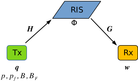
A transmitter equipped with antennas and a receiver equipped with antennas communicate through an RIS. A single-stream transmission is adopted, in order to exploit the diversity gain ensured by the presence of the RIS and of the multiple transmit and receive antennas11 1 A more general scenario is represented by a multi-stream transmission, which trades-off reliability with throughput. However, this scenario would lead to more cumbersome expressions of the rate and energy efficiency functions and is left as future work.. The case under analysis models point-to-point links, but also downlink or uplink communications in cellular networks where multi-user interference is suppressed (for example by means of any orthogonal signaling protocols such as frequency or time division multiple access, or by orthogonal frequency division multiple access).
We assume that no direct link between the transmitter and receiver exists, and we denote by and the channels from the transmitter to the RIS and from the RIS to the receiver, respectively, by the unit-norm transmit beamformer, and by the unit-norm receive combiner. Among the different implementations of RISs [11, 52], we consider surfaces that are made of large arrays of inexpensive antennas that are spaced half of the wavelength apart and that are individually controlled and tuned. More specifically, we assume that the RIS is made of elementary individually and locally optimized passive scatterers, which are capable of independently reflecting the radio wave impinging upon them, by applying a phase shift denoted by , with , which we collect in the diagonal matrix . Thus, in this paper the RIS is employed for channel-aware beamforming through the environment.
Before the data transmission phase starts, it is necessary to estimate the channels and , and to configure the optimized phase shifts at the RIS. More details on channel estimation and RIS phase shifts configuration are provided in Section III-D. Nevertheless, at this stage it is important to stress that both channel estimation and resource optimization can be performed either at the transmitter or at the receiver, but not at the RIS. On the other hand, the RIS is interfaced with the transmitter through a controller with minimal signal processing, transmission/reception, and power storage capabilities. The transmission/reception capabilities are needed in order to receive the configuration signals from the transmitter. The signal processing capabilities are needed in order to decode the configuration signals and configure the phase shifts of the RIS. The power storage capabilities are needed in order to operate the electronic circuits (switches or varactors) that make the surface reconfigurable. The controller is a key element to ensure the dynamic reconfigurability of the RIS, as a function of the propagation channel [11, Figure 4]. However, feeding back the optimized phase matrix to the RIS before the data transmission phase, may introduce a non-negligible overhead to the communication phase, especially for large . Let us denote by the duration of the feedback phase, which depends on the power used during the feedback phase and on the bandwidth of the feedback channel. Moreover, let us denote by the duration of the channel estimation phase prior to feedback and communication. Mathematical expressions of and are provided in Section III-D. Then, denoting by the total duration of the time slot comprising channel estimation, feedback, and data communication, the system achievable rate and energy efficiency are expressed as
| (1) | ||||
| (2) |
wherein denotes the total power consumption in the whole timeframe , which is equal to
| (3) |
since a power is used for seconds, with transmit amplifier efficiency , a power is used for seconds, with transmit amplifier efficiency , while a hardware static power is consumed for the whole interval , and accounts for the energy consumption for channel estimation, which is further detailed in Section III-D. This work optimizes the transmit and feedback powers and bandwidths , the RIS matrix , and the precoding and decoding vectors , in order to maximize the rate (II), the energy efficiency (2), and derive the rate-energy Pareto-region.
III Optimization of , ,
As a first step, let us fix , and focus on optimizing the RIS phase matrix , the unit-norm beamforming vector , and the unit-norm decoding vector . Since do not appear in the denominator of the energy efficiency, but only in the numerator, which coincides with the system rate, both rate and energy efficiency maximization are cast as
| (4) |
Denoting by the largest singular value of , it holds
| (5) |
where we have used Cauchy-Schwarz inequality, the constraint that , and the fact that the maximum of with respect to the set of unit-norm vectors is the spectral norm of , i.e. the largest singular value of , [53, pag. 148]. Then, for any , the optimal and are the dominant right and left eigenvector of , since this achieves the upper-bound in (III). However, optimally maximizing the largest singular value of with respect to appears prohibitive. Moreover, this would not yield any closed-form expression for , , , which hinders the analytical evaluation of the ultimate performance of RIS-based networks. Thus, we propose two closed-form approaches for optimizing an upper-bound or a lower-bound of the objective of (4).
III-A Optimizing an upper-bound of the objective of (4)
Let , be the singular values decompositions (SVDs) of and , with , . Then, it holds that
| (6) |
wherein Inequality is due to the triangle inequality, while Inequality is a special case of Cauchy-Schwarz inequality.22 2 Cauchy-Schwarz inequality states that , for any non-negative numbers . Then, by taking for all , we obtain In the following, we derive a closed-form solution for the maximization of the bound in (6) with respect to , , . We start with the following lemma.
Lemma 1
Consider and for all , with . Then it holds that , with such that for all .
Proof:
Since for all , there exist non-negative such that , for all . Then, the result is shown as follows
∎The optimal , , for the upper-bound in (6) are as follows.
Proposition 1
For any , defining
| (7) | ||||
| (8) |
the global maximizer of the upper-bound in (6) is obtained by setting , , and , with (∗) denoting complex conjugate.
Proof:
Neglecting the inessential factors , we observe that
| (9) | ||||
wherein the inequality follows upon taking the maximum over . Next, for any , the term defined in the last line of (9) can be upper-bounded as
| (10) |
wherein (b) follows because, for any , the optimal is the one that compensates the phase shifts between the components of and of , while (a) follows from Lemma 1 because , since, for all , is the projection of the unit-norm vector onto the unit-norm vector . Plugging (III-A) into (9), yields
| (11) |
wherein the last inequality holds by Lemma 1. Finally, the result follows since all inequalities hold with equality upon choosing as in the thesis of the proposition. ∎
III-B Optimizing a lower-bound of the objective of (4)
Define , , and observe that, for any fixed and , the optimal for Problem (4) is such that , for all . Next, denoting by and the -th row of and the -th column of , respectively, with , it holds that and . Then, we obtain
| (12) | ||||
where follows by using the maximizer with respect to , i.e. , and is due to the triangle inequality. Then, by similar steps as those that led to (III), the final maximization is obtained when are the dominant right and left eigenvector of .
III-C Tackling (4) by alternating maximization
As a benchmark solution, let us maximize by alternatively optimizing , for fixed , and then , for fixed . For fixed , the optimal and are derived as the dominant left and right eigenvectors of the matrix , as shown in (III). Instead, for fixed and , the problem amounts to maximizing , which yields , for all , as shown in Section III-B. Thus, alternating maximization leads to Algorithm 1.
III-D Overhead modeling
This section derives a mathematical expression for , , . Without loss of generality, we assume that channel estimation and resource optimization takes place at the transmitter.33 3 A similar argument would hold in the case in which channel estimation and resource optimization took place at the receiver.
As for , after resource optimization, the transmitter sends a control signal to the RIS to configure the phase shifts.44 4 Here we neglect the feedback of the receive filter to the receiver, because, first it is negligible with respect to the feedback of the RIS phase shifts, since typically , and, second, because the focus of this work is on the RIS and on evaluating the feedback required to operate it. Denoting by the scalar feedback channel from the RIS to the transmitter, it holds that , with the number of feedback bits for each reflecting element of the RIS and the noise power spectral density. As anticipated, depends on , , which complicates the mathematical structure of the rate in (II) and the energy efficiency in (2), complicating the optimization of these two metrics, and of their trade-off, with respect to . The optimization of for the maximization of the rate, the energy efficiency, and their trade-off is addressed in Section IV.
As for , it is affected by the specific channel estimation protocol in use. As an example, we consider that the pilot tones are sent by the receiver to the transmitter, but a similar analysis applies to the case in wich the transmitter send pilot tones to the receiver. Moreover, we consider that, during the estimation phase, the RIS does not apply any phase shift, i.e. for all , [54]. In the following, two different channel estimation protocols are considered:
- (a)
Let us consider the simple case in which the receiver sends pilot tones sequentially, one after the other, to the transmitter, through the RIS. Thus, the product channels are estimated sequentially, with denoting the channel from the -th transmit antenna to the -th RIS elements, and denoting the channel from the -th RIS element to the -th receive antenna. Moreover, one additional pilot tone is required for the transmitter to estimate the feedback channel. Therefore, denoting by the duration of each pilot tone, it holds . It should be remarked that the knowledge of the product channels is enough to reconstruct the matrix in (III) and, therefore, to optimally solve (4) with respect to the phase shifts of the RIS, the beamforming vector, and the receive filter. Finally, the energy consumption for channel estimation can be modeled as , with the power of each pilot tone. In particular, the overhead needed for channel estimation is estimated based on the channel state information needed to optimally solve (4). However, our algorithms work also with recently proposed channel estimation algorithms, e.g., [54].
- (b)
The case in which the receiver transmits orthogonal pilots in parallel, which are jointly processed at the transmitter. Then, for all , the pilot from the -th antenna of the receiver allows estimating the product channels , for all and . Thus, in this case it holds , since all pilots are transmitted at the same time. On the other hand, , because the pilots are transmitted at the same time, each with power .
Thus, based on the expressions of and , the power consumption in (3) becomes
IV Optimization of .
After optimizing by any of the methods developed in Section III, we are left with the problem of optimizing the transmit powers , and the bandwidths . It should be stressed that, as already mentioned, the optimized that are obtained from any of the algorithms developed in Section III, do not depend on any of the variables , but only on the channels and . Moreover, as already mentioned, the optimized are the same for both the rate and the energy efficiency. Thus, it is possible to simply plug in the optimized into the objective to maximize, thus effectively decoupling the optimization of from the optimization of . On the other hand, unlike , the optimization of depends on whether the goal is optimizing the rate, the energy efficiency, or their trade-off. Therefore, these problems are treated separately.
IV-A Rate maximization
The rate maximization problem is stated as the following optimization program
| (13a) | ||||
| (13b) | ||||
| (13c) | ||||
| (13d) | ||||
Expressing (13a) as a function of the optimization variables yields
| (14) |
wherein and . Thus, being the product of two functions, the objective of (13) is not jointly concave in all optimization variables, which makes Problem (13) challenging to solve with affordable complexity. Indeed, the product of functions is in general not concave even in the simple case in which the individual factors are concave. Moreover, in the case at hand, the concavity of the two factors defining (IV-A) is not clear, either. Thus, in order to solve (13), it is not possible to directly use standard convex optimization algorithms. In the rest of this section we show that it is possible to reformulate Problem (13) into a convex optimization problem without any loss of optimality. To this end, some preliminary lemmas are needed.
Lemma 2
The function is jointly increasing and jointly concave in .
Proof:
Neglecting inessential constant terms (with respect to and ), and defining
| (15) |
Eq. (13a) is equivalent to the function , which is the perspective of the concave function [55]. Thus, since the perspective operator preserves concavity, is jointly concave in . Moreover, is clearly increasing in , while inspecting the derivative of with respect to , and exploiting that for any , shows that is increasing in . ∎
Lemma 3
The function is jointly increasing and jointly concave in .
Proof:
Neglecting inessential constant terms (with respect to and ), it can be seen that, upon defining , the function in (13a) is equivalent to
| (16) |
Showing the joint concavity of (16) with respect to is equivalent to showing that the function , is jointly convex in . After some elaborations, the Hessian matrix of is written as given in (17), shown at the top of the next page,
| (17) | ||||
wherein is the first-order derivative of with respect to . Clearly, the entry of is non-negative. Thus, is positive semi-definite if its determinant is non-negative. Then, since the second derivative of with respect to can be written as
| (20) |
after some elaborations, enforcing that the Hessian of is non-negative leads to the condition . This holds if , which is true by virtue of the inequality . Moreover, implies that is increasing in , while it is clearly increasing in . ∎
Leveraging Lemmas 2 and 3, it is possible to equivalently reformulate Problem (13) into a convex problem, which can then be efficiently solved by means of any convex optimization method. To this end, the first step is to observe that taking the logarithm of the objective in (13a) does not change the optimal solutions of (13a), since the logarithm is an increasing function. Then, an equivalent reformulation of (13a) is the following problem
| (21a) | ||||
| (21b) | ||||
| (21c) | ||||
| (21d) | ||||
which is a convex optimization problem by virtue of Lemmas 2 and 3. Indeed, (21a) is a concave function since Lemmas 2 and 3 ensure that both summands are concave. Also, all the constraints in (21b)-(21c) are linear, while (21d) is convex thanks to Lemma 3. Thus, Problem (21) is a convex problem with the same set of solutions as Problem (13), but the advantage that it can be solved by convex optimization theory.
Finally, in order to further simplify the solution of (21), we observe that the optimal solution of (21) is such that (21b) and (21c) must be fulfilled with equality, since the objective function is increasing in all arguments and (21d) is decreasing in both and . Thus, Problem (21) can be reformulated, without loss of optimality, as
| (22a) | ||||
| (22b) | ||||
| (22c) | ||||
which has only two optimization variables. Upon solving (22), the optimal feedback power and bandwidth are retrieved as and . Problem (22) is clearly still a convex problem, since it is obtained from the convex Problem (21) upon applying the linear variable transformations and , and linear transformations are well-known to preserve convexity. Finally, after developing a method for solving (22) with affordable complexity, in the last part of this section we focus on obtaining closed-form solutions for the special cases of Problem (22) obtained by considering the optimization of the transmit powers for fixed bandwidths and vice-versa. Closed-form solutions can be obtained as follows.
IV-A1 Optimization for fixed and
Fixing and , Problem (22) reduces to
| (23a) | ||||
| (23b) | ||||
Proposition 2
Let be the unique stationary point of (23a). Then, Problem (23) has a unique solution given by , with the unique solution of Eq. (24), shown at the top of this page.
| (24) |
Proof:
Equating the first-order derivative of (23a) to zero yields (24), which has always a solution, since the left-hand-side is decreasing in and tending to for , while the right-hand-side is increasing in , being finite at and tending to for . Then, (23a) has a unique solution , since (23a) is a strictly concave function in , as it is the sum of concave functions and is strictly concave in . Finally, (24) shows that (23a) is strictly increasing for and strictly decreasing for . Thus, we can conclude that the unique solution of Problem (23) is either , if , or it is itself. ∎Finally, it holds .
IV-A2 Optimization for fixed and
Fixing and , Problem (22) reduces to
| (25a) | ||||
| (25b) | ||||
with the unique55 5 The uniqueness holds because the function at the left-hand-side is strictly decreasing, as it immediately follows from previous results. value of that fulfills the following inequality with equality
| (26) |
Proposition 3
IV-B Energy efficiency optimization
Plugging again any of the allocations of developed in Section III into the energy efficiency function, leads us to the following problem to solve
| (28a) | ||||
| (28b) | ||||
| (28c) | ||||
| (28d) | ||||
It should be stressed that, in order to solve (28), it is not possible to employ the same approach used for rate maximization, because the presence of the denominator makes the logarithm of (28a) not jointly concave in all optimization variables. Moreover, standard fractional programming algorithms are not directly applicable since they have limited complexity only when the numerator and the denominator of the objective to maximize are concave and convex functions, respectively. Unfortunately, in (28), neither the concavity of the numerator, nor the convexity of the denominator hold. Finally, a third issue that makes (28) more challenging than the rate optimization problem is that, unlike the rate function, (28a) is not monotonically increasing in either or , and so it can not be guaranteed that, at the optimum, it holds . On the other hand, (28a) is increasing in and , since, as shown in Section IV, the numerator is increasing in and , while the denominator depends only on and decreases with . Thus, at the optimum holds. Exploiting this and defining
| (29) |
(28) can be cast as
| (30a) | ||||
| (30b) | ||||
| (30c) | ||||
| (30d) | ||||
wherein , and is given in (15). Next, we also consider a relaxed version of (30) in which (30d) is reformulated into an inequality constraint, namely
| (31a) | ||||
| (31b) | ||||
| (31c) | ||||
| (31d) | ||||
which, unlike (30), has a convex feasibility set, thanks to the fact that the first constraint in (30d) is an inequality constraint wherein the right-hand-side is a concave function. An important result is that, as shown in the coming proposition, (30) and (31) are equivalent problems.
Proof:
The result follows by showing that any optimal solution of (31) is such that . To this end, let us observe that (31a) is monotonically increasing in . Indeed, by dividing numerator and denominator by , (31a) can be equivalently expressed as , which is strictly increasing in . Based on this, the result follows proceeding by contradiction. Specifically, if were a solution of (31), but , then it would be possible to find a feasible . Since (31a) is increasing in , would yield a larger objective value than , thus contradicting the fact is a solution of (31). ∎Despite having a convex feasibility set, Problem (31) is still challenging to solve, since the numerator and denominator of (31a) are not concave and convex functions, respectively, which prevents one from using fractional programming techniques. However, recalling Lemma 2, fractional programming can be used if is fixed. More precisely, for any fixed , Problem (31) is an instance of a so-called pseudo-concave maximization problem, in which the fraction to maximize has a concave numerator and an affine denominator, and thus can be solved with limited complexity by any fractional programming method, such as the popular Dinkelbach’s method [56]. Moreover, from (31d), it must hold that
| (32) |
Based on these considerations, Problem (31d) can be solved by performing a line search over in the interval given by (32), and solving, for each considered value , the corresponding pseudo-concave maximization problem as follows
| (33a) | ||||
| (33b) | ||||
| (33c) | ||||
| (33d) | ||||
Thus we have Algorithm 2, wherein denotes the value of (33a) obtained at the -th iteration.
IV-C Rate-EE optimization
This section focuses on characterizing the rate-energy Pareto-optimal frontier of the bi-objective problem that has as objectives the system rate and the energy efficiency.
To begin with, since affect only the numerator of the energy efficiency, which coincides with the rate, we can plug any of the allocations of developed in Section III into the rate and the energy efficiency functions, which yields
| (35a) | ||||
| (35b) | ||||
| (35c) | ||||
where we have already exploited the fact that at the optimum it must hold . With respect to the other variables, on the other hand, the rate and energy efficiency are in general maximized by different resource allocations. Clearly, this is the scenario in which Problem (35) is of interest, because otherwise no trade-off would exist between the two functions, and the solution of Problem (35) would be trivially equal to the common maximizer of the rate and of the energy efficiency.
The most widely-used solution concept for bi-objective problems like (35) is that of Pareto-optimality. A Pareto-optimal solution of (35a) is a point lying on the so-called Pareto-frontier of the problem, defined as the set of resource allocations for which it is not possible to further increase either one of the two objectives, without decreasing the other objective. To elaborate further, let us denote by and the maximum rate and energy efficiency that can be computed as shown in Sections IV-A and IV-B, respectively. Then, we also denote by the rate obtained with the resource allocation that maximizes the energy efficiency, and by the energy efficiency obtained with the resource allocation that maximizes the rate. Then, it follows that the extreme points of the Pareto-frontier in the plane are and . As expected, this also shows that the Pareto-frontier degenerates into a single point when the rate and the energy efficiency admit the same maximizer. Instead, in general a non-trivial Pareto-frontier exists for (35), which provides all optimal trade-off points between the rate and the energy efficiency. Focusing on this scenario, multi-objective optimization theory provides several approaches to compute all Pareto-optimal points of a multi-objective problem. One of the most widely-used methods is the maximization of the minimum between a weighted combination of the objectives. As for Problem (35), introducing the auxiliary variable defined in (29), the max-min approach leads to the problem:
| (36a) | ||||
| (36b) | ||||
| (36c) | ||||
wherein we have plugged in the expression of the energy efficiency, with , is a non-negative parameters that weighs the relative importance between the rate and the energy efficiency, while and are the maximum of the rate and of the energy efficiency, respectively. For any , (36) has at least one solution that is Pareto-optimal for (36) [57, Theorem 3.4.3], and solving (36) for all yields all the points on the Pareto-frontier of (35) [57, Theorem 3.4.5]. Also, the two extreme points and correspond to the single-objective maximization of the rate and of the energy efficiency. In order to solve (36), we consider its equivalent reformulation in epigraph form, namely
| (37a) | ||||
| (37b) | ||||
| (37c) | ||||
| (37d) | ||||
| (37e) | ||||
| (37f) | ||||
Solving (36) is challenging due to the presence of the variable . However, for any fixed , (36) can be conveniently solved by employing the bisection algorithm over , since all constraint functions are convex in all other variables. Specifically, observing that must lie in the interval defined by (32), Problem (37) can be solved by performing a line search over , solving in each iteration the following problem with lying in in the interval defined by (32):
| (38a) | ||||
| (38b) | ||||
| (38c) | ||||
| (38d) | ||||
| (38e) | ||||
| (38f) | ||||
Problem (36) can be solved similarly as in Algorithm 2. Formally, this yields Algorithm 3.
V Optimality properties and computational complexity
This section analyzes the properties and complexity of the proposed optimization algorithms. The algorithms developed in Sections III-A and III-B are discussed in Section V-A, while those developed in Section IV are discussed in Section V-B.
V-A Algorithms for the optimization of , ,
The algorithms for the optimization of the RIS phase shifts, the transmit beamforming, and the receive vector introduced in Sections III-A and III-B are based on the use of upper and lower bounds of the receive signal-to-interference-plus-noise ratio (SINR). As a result, in general they are not globally optimal. Nevertheless, they achieve global optimality whenever the rank of and are equal to one. Indeed, in this case both the upper-bound in Section III-A and the lower-bound in Section III-B are tight, because when , the vectors and reduce to scalars. The case of rank-one channles includes two notable special cases:
- •
The case in which a single-antenna is used at the transmit and receive side.
- •
The use of mmWave communications, which, in many cases, leads to rank-one channels as all energy is focused in a pencil-beam transmission.
In general, as we have explained at the beginning of Section III, jointly optimizing , , and in a globally optimal way is computationally prohibitive due to the lack of a tractable and closed-form expression for the dominant singular value of the matrix . As a result, the global joint optimization of , , and would require an exhaustive search in an -dimensional space. This justifies the use of possibly sub-optimal optimization methods, among which the state-of-the-art approach is the alternating optimization algorithm reviewed in Section III-C. Here, we show that the two novel approaches developed in Sections III-A and III-B require a lower computational complexity than alternating optimization.
To elaborate, alternating optimization is an iterative approach, which requires to compute, in each iteration of the algorithm, the SVD of the matrix , as well as the vectors and to set the RIS phase shifts to , for all . Thus, if is the number of iterations until the alternating optimizations converges, the above operations are to be executed times. Instead, the advantage of our proposed methods is that they are not iterative, but are based on closed-form optimization results. Specifically, both methods from Sections III-A and III-B require the computation of a single SVD and a single RIS phase adjustment of the form . In addition, the method developed in Section III-A requires two searches over finite sets of size and , respectively, while the method developed in Section III-B requires computing the matrix . Again, all of these additional operations are to be executed only once, and their complexity is negligible compared to that of performing an SVD. In summary, since the proposed algorithms are not iterative, but are based on closed-form optimization expressions, they reduce the complexity compared to alternating optimization by a factor . Moreover, Section VI will numerically show that the proposed methods perform very close to alternating optimization.
V-B Algorithms for the optimization of , , ,
All algorithms developed for the optimization of the transmit and feedback power and bandwidths are globally optimal and require a limited computational complexity. Specifically:
- •
Rate optimization has been recast as a concave maximization, which is optimally solvable with polynomial complexity in the number of optimization variables [55].
- •
The energy efficiency maximization problem has been reformulated as a pseudo-concave maximization problem upon fixing the value of the auxiliary variable . Thus, energy efficiency maximization can be optimally performed by a scalar line search over and by solving a pseudo-concave maximization problem for each considered value of . Recalling that polynomial complexity algorithms exist to solve pseudo-concave maximizations [58], the complexity of energy efficiency maximization is polynomial in the number of optimization variables, and linear in the number of points used for the line search.
- •
The bi-objective problem of rate and energy efficiency maximization has been reformulated as the feasibility test in (37), that can be optimally solved by a sequence of feasibility tests of the form of Problem (38), which become convex when fixing the variable . Thus, the complexity of rate and energy efficiency bi-objective maximization is polynomial in the number of optimization variables, and linear in the number of points used for the line search. Moreover, the optimal parameter is determined by a bisection search, which requires solving (38) times, with and the initialization of the bisection method, and the accuracy of the bisection search [55].
VI Numerical Results
| 45 / 45 / 10 dBm | 100 MHz | -174 dBm/Hz | 1 / 1 | 16 bit |
For all , , , each product channel is generated as , wherein and are realizations of two independent complex circularly symmetric standard Gaussian variable, while accounts for the overall path-loss and shadowing effects from the transmitter to the RIS and from the RIS to the receiver66 6 Rayleigh fading is a suitable case study in scenarios in which the location of the RIS can not be optimized and the existence of a strong line-of-sight component can not be guaranteed. This is the case when the RISs are randomly deployed, e.g., on spatial blockages whose locations are not under the control of the system designer.. In our simulations, we set , with . A similar model is used for the feedback channel .
Figs. 2-9 assume that the overhead model from Section III-D, Case (a), is employed. Figure 2 plots the maximum rate in (II) (normalized by ) versus , with , (Fig. 2-a), and (Fig. 2-b), for:
- (a)
obtained from the optimal method from Section IV, with , and , chosen as the dominant right and left eigenvectors of . Thus, the RIS simply reflects the signal without any phase manipulation. It is worth noting that in this case there is no need to configure the phase shifts of the RIS, and, therefore, the total overhead is much reduced. In particular, the numerical results that correspond to this case are obtained by setting and .
- (b)
- (c)
- (d)
The results in Figure 2 indicate that the proposed schemes are able to outperform the case in which no RIS optimization is performed, which shows that the use of RISs can significantly improve the system performance, even if the overhead for channel estimation and system configuration is taken into account. Moreover, it is observed that the proposed closed-form Schemes (b) and (c) offer similar performance as alternating optimization, which instead requires the implementation of an iterative numerical algorithm. Indeed, we recall that when , Schemes (b) and (c) are provably optimal.


In order to show the impact of the overhead that is necessary to operate RIS-empowered wireless networks, Figure 3 considers a similar scenario as in Figure 2, with the only difference that the number of receive antennas is set to , which significantly increases the amount of feedback data. As a result, it is observed that the gap between Schemes (b), (c), (d), which optimize the phase shifts of the RIS, and Scheme (a) without RIS optimization, gets smaller, since not optimizing the phases allows one to dispense with the overhead to obtain the channels and for each individual phase shift. Also, the gap is smaller when a larger is considered, since a longer time is needed for channel estimation and feedback. Moreover, it is interesting to observe that Scheme (b) performs similar to alternating optimization, despite requiring a much lower computational complexity thanks to the fact that it provides a closed-form allocation. On the other hand, Scheme (d) shows a slight gap compared to Schemes (b) and (d).


The trend displayed in Figure 3 becomes even more significant in Figure 4, where the number of antennas is further increased by considering . In this case, Scheme (a) which does not require any overhead for the optimization of the RIS phase shifts, outperforms the system setup in the presence of an RIS, when , i.e., when a longer time is used for channel estimation. Instead, when a shorter channel estimation time is used, i.e., when , performing radio resource allocation is still beneficial up to , whereas not using an RIS becomes better for higher values of . Moreover, also in this case Schemes (b) and (d) perform very similarly, while Scheme (c) exhibits a slight gap.


The obtained results motivate the use of RISs in scenarios with a low number of transmit and receive antennas, especially for large . Indeed, for any additional antenna that is deployed, new channels must be estimated and the optimized phases need to be communicated to the RIS. Comparing the performance of the optimized schemes in Figures 2 and 3 reveals that deploying a moderate number of antennas does not lead to improved performance. Indeed, the presence of an RIS may make transmit beaforming and receive combining not necessary. This finding agrees with recent results from [59].
Similar considerations hold for the case in which the energy efficiency is optimized, as it emerges from Figures 5, 6, 7, which consider the same four schemes considered in Figures 2, 3, 4, respectively, with the only differences that have been allocated for energy efficiency maximization, according to the optimal method from Section IV-B. Also, two values of are considered, namely and . In this case, Scheme (a) without any RIS feedback transmission starts performing better than the optimized schemes that rely on feedback transmissions when , , , and , i.e., for a lower overhead than for rate optimization. This can be explained since in the case of energy efficiency optimization, feedback overheads do not affect only the rate function, but also the power consumption at the denominator of the energy efficiency in (28a). Finally, Figures 8 and 9 consider again Schemes (a)-(d), with allocated for rate-energy bi-objective maximization according to the optimal method from Section IV-C. The system rate-energy Pareto boundary is shown for the two cases: (1) ; (2) , with . Similar remarks as for previous scenarios hold.
Next, Figures 10, 11, 12 consider the overhead model in which the receiver transmit orthogonal pilots at the same time, as described in Section III-D, and show the achieved spectral efficiency, energy efficiency, and their optimal trade-off, for the case without RIS (Scheme (a)) and the use of Scheme (b) (similar results are obtained for Schemes (c) and (d), but results are omitted for brevity). Only the case and is considered, as this is the most difficult scenario for the proposed method since a longer time and more power are spent for each pilot tone. Despite the challenging scenario, Figure 10 shows that the slightly more sophisticated feedback scheme ensures that the use of an optimized RIS provides higher spectral efficiency in both cases and . Similar results are shown in Figure 11 for the energy efficiency, with the difference that RIS optimization becomes not convenient when and , since transmitting the pilots simultaneously does not remove the factor in the term . Finally, Figure 12 shows that RIS optimization improves the spectral energy trade-off when (and thus also when ), for and .


VII Conclusions
A framework for overhead-aware radio resource allocation in RIS-aided systems has been developed for spectral and energy efficiency optimization. Two new closed-form methods for the optimization of the RIS phase shifts, as well as of the transmit and receive vectors, have been developed. Moreover, the transmit powers and bandwidths for the communication and feedback phases have been globally optimized through concave/pseudo-concave maximizations. The derived results indicate that RIS constitutes a suitable technology when suitable feedback mechanisms are used or when few transmit and receive antennas are deployed, since a trade-off exists between optimizing the network radio resources and the overhead due to the deployment of the optimized solution. In particular, there exists a limit to the number of antennas and RIS reflectors, before feedback overhead makes radio resource optimization not convenient compared to the setup where RISs are not deployed. An important future line of investigation is the analysis of the impact of multi-user interference on overhead-aware resource allocation in RIS-based networks. Multi-user interference complicates the resource allocation problems, possibly requiring the use of numerical optimization techniques.
References
- [1] A. Gatherer, “What will 6G be?” https://www.comsoc.org/publications/ctn/what-will-6g-be, 2018.
- [2] J. G. Andrews, “Seven ways that hetnets are a cellular paradigm shift,” IEEE Communications Magazine, vol. 51, no. 3, pp. 136–144, 2013.
- [3] T. L. Marzetta, “Noncooperative cellular wireless with unlimited numbers of base station antennas,” IEEE Transactions on Wireless Communications, vol. 9, no. 11, pp. 3590–3600, 2010.
- [4] T. S. Rappaport et al., “Millimeter wave mobile communications for 5G cellular: It will work!” IEEE Access, vol. 1, pp. 335–349, 2013.
- [5] J. Andrews, S. Buzzi, W. Choi, S. Hanly, A. Lozano, A. C. K. Soong, and J. C. Zhang, “What will 5G be?” IEEE Journal on Selected Areas in Communications, vol. 32, no. 6, pp. 1065–1082, June 2014.
- [6] 5G PPP, “5GPPP vision on software networks and 5G SN WG,” https://5g-ppp.eu/wp-content/uploads/2014/02/5G-PPP_SoftNets_WG_whitepaper_v20.pdf, 2017.
- [7] P. Popovski, K. F. Trillingsgaard, O. Simeone, and G. Durisi, “5G wireless network slicing for eMBB, URLLC, and mMTC: A communication-theoretic view,” IEEE Access, vol. 6, pp. 55 765–55 779, 2018.
- [8] A. Zappone, M. Di Renzo, and M. Debbah, “Wireless networks design in the era of deep learning: Model-based, AI-based, or both?” IEEE Trans. on Commun., vol. 67, no. 10, pp. 7331–7376, October 2019.
- [9] L. Subrt and P. Pechac, “Controlling propagation environments using intelligent walls,” European Conf. on Antennas and Propagation, 2012.
- [10] M. Di Renzo et al., “Smart radio environments empowered by reconfigurable AI meta-surfaces: An idea whose time has come,” EURASIP Journal on Wireless Communincations and Networking, vol. 129, 2019.
- [11] M. Di Renzo, A. Zappone, M. Debbah, M. Alouini, C. Yuen, J. de Rosny, and S. Tretyakov, “Smart radio environments empowered by reconfigurable intelligent surfaces: How it works, state of research, and road ahead,” IEEE Journal on Selected Areas in Communications, 2020.
- [12] N. Yu et al., “Light propagation with phase discontinuities: Generalized laws of reflection and refraction,” Science, vol. 334, no. 6054, 2011.
- [13] F. Liu et al., “Programmable metasurfaces: State of the art and prospects,” IEEE Intern. Symposium on Circuits and Systems, 2018.
- [14] C. Liaskos et al., “Realizing wireless communication through software-defined hypersurface environments,” IEEE International Symposium on World of Wireless, Mobile and Multimedia Networks, 2018.
- [15] M. Di Renzo et al., “Analytical modeling of the path-loss for reconfigurable intelligent surfaces - anomalous mirror or scatterer,” https://arxiv.org/pdf/2001.10862.pdf, 2020.
- [16] V. S. Asadchy et al., “Perfect control of reflection and refraction using spatially dispersive metasurfaces,” Phy. Review B, vol. 94, no. 7, 2016.
- [17] A. Diaz-Rubio, V. S. Asadchy, A. Elsakka, and S. A. Tretyakov, “From the generalized reflection law to the realization of perfect anomalous reflectors,” Science Advances, vol. 3, no. 8, 2017.
- [18] C. Liaskos et al., “A new wireless communication paradigm through software-controlled metasurfaces,” IEEE Communications Magazine, vol. 56, no. 9, pp. 162–169, 2018.
- [19] Q. Wu and R. Zhang, “Towards smart and reconfigurable environment: Intelligent reflecting surface aided wireless network,” IEEE Communications Magazine, 2019.
- [20] E. Basar et al., “Wireless communications through reconfigurable intelligent surfaces,” IEEE Access, vol. 7, pp. 116 753–116 773, 2019.
- [21] C. Huang et al., “Holographic MIMO surfaces for 6G wireless networks: Opportunities, challenges, and trends,” https://arxiv.org/pdf/1911.12296.pdf, 2019.
- [22] S. Hu, F. Rusek, and O. Edfors, “Beyond massive mimo: The potential of data transmission with large intelligent surfaces,” IEEE Transactions on Signal Processing, vol. 66, no. 10, pp. 2746–2758, May 2018.
- [23] N. Shlezinger et al., “Dynamic metasurface antennas for uplink massive mimo systems,” IEEE Transactions on Communications, vol. 67, no. 10, pp. 6829–6843, October 2019.
- [24] M. Di Renzo et al., “Reconfigurable intelligent surfaces vs. relaying: Differences, similarities, and performance comparison,” https://arxiv.org/abs/1908.08747, 2019.
- [25] X. Lu et al., “Intelligent reflecting surface (IRS)-enabled covert communications in wireless networks,” https://arxiv.org/abs/1911.00986, 2019.
- [26] N. Kaina, M. Dupre, G. Lerosey, and M. Fink, “Shaping complex microwave fields in reverberating media with binary tunable metasurfaces,” Scientific Reports, Article ID 6693, vol. 4, 2014.
- [27] G. Lavigne et al., “Susceptibility derivation and experimental demonstration of refracting metasurfaces without spurious diffraction,” IEEE Trans. on Antennas and Prop., vol. 66, no. 3, pp. 1321–1330, 2018.
- [28] W. Tang et al., “Wireless communications with programmable metasurface: Transceiver design and experimental results,” China Communications, vol. 16, no. 5, pp. 46–61, May 2019.
- [29] ——, “Programmable metasurface-based RF chain-free 8PSK wireless transmitter,” IEEE Electronic Letters, vol. 55, no. 7, pp. 417–420, 2019.
- [30] L. Dai et al., “Reconfigurable intelligent surface-based wireless communication: Antenna design, prototyping and experimental results,” https://arxiv.org/pdf/1912.03620.pdf, 2019.
- [31] C. Huang, A. Zappone, G. C. Alexandropoulos, M. Debbah, and C. Yuen, “Reconfigurable intelligent surfaces for energy efficiency in wireless communication,” IEEE Trans. on Wireless Commun., vol. 18, no. 8, pp. 4157–4170, 2019.
- [32] Q. Wu and R. Zhang, “Intelligent reflecting surface enhanced wireless network: Joint active and passive beamforming design,” IEEE Trans. on Wireless Commun., vol. 18, no. 11, pp. 5394–5409, November 2019.
- [33] Y. Yang, S. Zhang, and R. Zhang, “IRS-enhanced OFDM: Power allocation and passive array optimization,” arxiv.org/1905.00604, 2019.
- [34] X. Yu, D. Xu, and R. Schober, “MISO wireless communication systems via intelligent reflecting surfaces,” in 2019 IEEE/CIC International Conference on Communications in China (ICCC), 2019.
- [35] H. Guo, Y.-C. Liang, J. Chen, and E. G. Larsson, “Weighted sum-rate optimization for intelligent reflecting surface enhanced wireless networks,” https://arxiv.org/pdf/1905.07920.pdf, 2019.
- [36] T. Jiang and Y. Shi, “Over-the-air computation via intelligent reflecting surfaces,” https://arxiv.org/pdf/1904.12475.pdf, 2019.
- [37] J. Chen, Y.-C. Liang, Y. Pei, and H. Guo, “Intelligent reflecting surface: A programmable wireless environment for physical layer security,” IEEE Access, vol. 7, pp. 82 599–82 612, June 2019.
- [38] M. Cui, G. Zhang, and R. Zhang, “Secure wireless communication via intelligent reflecting surface,” IEEE Wireless Communication Letters, vol. 8, no. 5, pp. 1410–1414, October 2019.
- [39] H. Shen, W. Xu, S. Gong, Z. He, and C. Zhao, “Secrecy rate maximization for intelligent reflecting surface assisted multi-antenna communications,” IEEE Communications Letters, vol. 23, no. 9, pp. 1488–1492, September 2019.
- [40] X. Li, J. Fang, F. Gao, and H. Li, “Joint active and passive beamforming for intelligent reflecting surface-assisted massive MIMO systems,” https://arxiv.org/abs/1912.00728, 2019.
- [41] D. Ma, M. Ding, and M. Hassan, “Enhancing cellular communications for UAVs via intelligent reflective surface,” https://arxiv.org/abs/1911.07631, 2019.
- [42] R. Liu, H. Li, M. Li, and Q. Liu, “Symbol-level precoding design for intelligent reflecting surface assisted multi-user MIMO systems,” https://arxiv.org/abs/1909.01015, 2019.
- [43] B. Ning, Z. Chen, W. Chen, and J. Fang, “Intelligent reflecting surface design for MIMO system by maximizing sum-path-gains,” https://arxiv.org/abs/1909.07282, 2019.
- [44] H. Han et al., “Intelligent reflecting surface aided network: Power control for physical-layer broadcasting,” arxiv.org/abs/1910.14383, 2019.
- [45] C. Pan, H. Ren, K. Wang, W. Xu, M. Elkashlan, A. Nallanathan, and L. Hanzo, “Multicell MIMO communications relying on intelligent reflecting surface,” https://arxiv.org/abs/1907.10864, 2019.
- [46] P. Wang, J. Fang, X. Yuan, Z. D. Chen, H. Duan, and H. Li, “Intelligent reflecting surface-assisted millimeter wave communications: Joint active and passive precoding design,” https://arxiv.org/abs/1908.10734, 2019.
- [47] C. You, B. Zheng, and R. Zhang, “Intelligent reflecting surface with discrete phase shifts: Channel estimation and passive beamforming,” https://arxiv.org/abs/1911.03916, 2019.
- [48] C. Pan, H. Ren, K. Wang, M. Elkashlan, A. Nallanathan, J. Wang, and L. Hanzo, “Intelligent reflecting surface aided MIMO broadcasting for simultaneous wireless information and power transfer,” IEEE Journal on Selected Areas in Communications, 2020.
- [49] G. Zhou, C. Pan, H. Ren, K. Wang, and A. Nallanathan, “A framework of robust transmission design for IRS-aided MISO communications with imperfect cascaded channels,” https://arxiv.org/abs/2001.07054, 2020.
- [50] S. Hong, C. Pan, H. Ren, K. Wang, K. Chai, and A. Nallanathan, “Robust transmission design for intelligent reflecting surface aided secure communication systems with imperfect cascaded CSI,” https://arxiv.org/abs/2004.11580, 2020.
- [51] G. Zhou et al., “Robust beamforming design for intelligent reflecting surface aided MISO communication systems,” Arxiv 1911.06237, 2020.
- [52] X. Qian, M. Di Renzo, J. Liu, A. Kammoun, and M.-S. Alouini, “Beamforming through reconfigurable intelligent surfaces in single-user MIMO systems: SNR distribution and scaling laws in the presence of channel fading and phase noise,” arxiv.org/pdf/2005.07472.pdf, 2020.
- [53] R. A. Horn and C. R. Johnson, Topics in Matrix Analysis. Cambridge University Press, 1991.
- [54] Z.-Q. He and X. Yuan, “Cascaded channel estimation for large intelligent metasurface assisted massive MIMO,” IEEE Wireless Communication Letters, vol. 9, no. 2, pp. 210–214, February 2019.
- [55] S. P. Boyd and L. Vandenberghe, Convex optimization. Cambridge Univ Press, 2004.
- [56] W. Dinkelbach, “On nonlinear fractional programming,” Management Science, vol. 13, no. 7, pp. 492–498, March 1967.
- [57] K. Miettinen, Nonlinear Multiobjective Optimization. Springer, 1999.
- [58] A. Zappone and E. Jorswieck, “Energy efficiency in wireless networks via fractional programming theory,” Foundations and Trends® in Communications and Information Theory, vol. 11, no. 3-4, pp. 185–396, 2015.
- [59] V. Arun and H. Balakrishnan, “RFocus: Practical beamforming for small devices,” https://arxiv.org/abs/1905.05130, 2019.