Role of Anisotropy in Nonlinear Harmonic Generation Across TMD MonolayersPreprint: ArXiV

TMDs are structures of the form MX₂, composed of a layer of a transition metal M interposed between two layers of a chalcogen X and with a typical thickness of around $6-7$Å. Depending on the metal’s group, their stacking arrangement can either be trigonal prismatic or octahedral. For group-VI metals, such as Mo and W, these three layers tend to stack in the former arrangement. This can be seen in Fig. 1(a), where the two species, which bond covalently, occupy either one of the two possible triangular sublattices, labelled $\mathbf{A}$ and $\mathbf{B}$, in a honeycomb lattice, effectively forming a monolayer if viewed from the top [Fig. 1(b)]. Due to weak van der Waals interlayer interactions, multilayer or bulk structures can be engineered. Extensive and detailed analysis of the chemical bonding mechanisms behind TMDs may be found in Kolobov and Tominaga 2016.

A TMD monolayer admits twelve symmetry operations, which are illustrated in Fig. 1. These consist of three 3-fold rotations around the black axis in Fig. 1(a), three 2-fold rotations around the axes laying on the horizontal plane, as shown in Fig. 1(b), two 3-fold improper rotations (composed of a 3-fold rotation followed by a reflection on the metal-occupied plane) and three reflections on their respective vertical planes. However, this structure lacks an inversion centre. To see why, the only hypothetical inversion centres, the centre of an arbitrary hexagon (labelled $\mathbf{P}$) and a lattice point $\mathbf{Q}$ are shown in Fig. 1(b). Inversion through $\mathbf{P}$ is not possible due to the alternate nature of each sublattice; as for $\mathbf{Q}$, only the lattice points of the same species are invertible (in this instance the metal species). This arrangement cannot therefore preserve inversion symmetry. The precise configuration of the TMD structure plays a role in the observation of this symmetry. Unlike monolayers, TMDs grown in bulk or multilayers of an even number of layers admit an inversion centre Kolobov and Tominaga 2016.

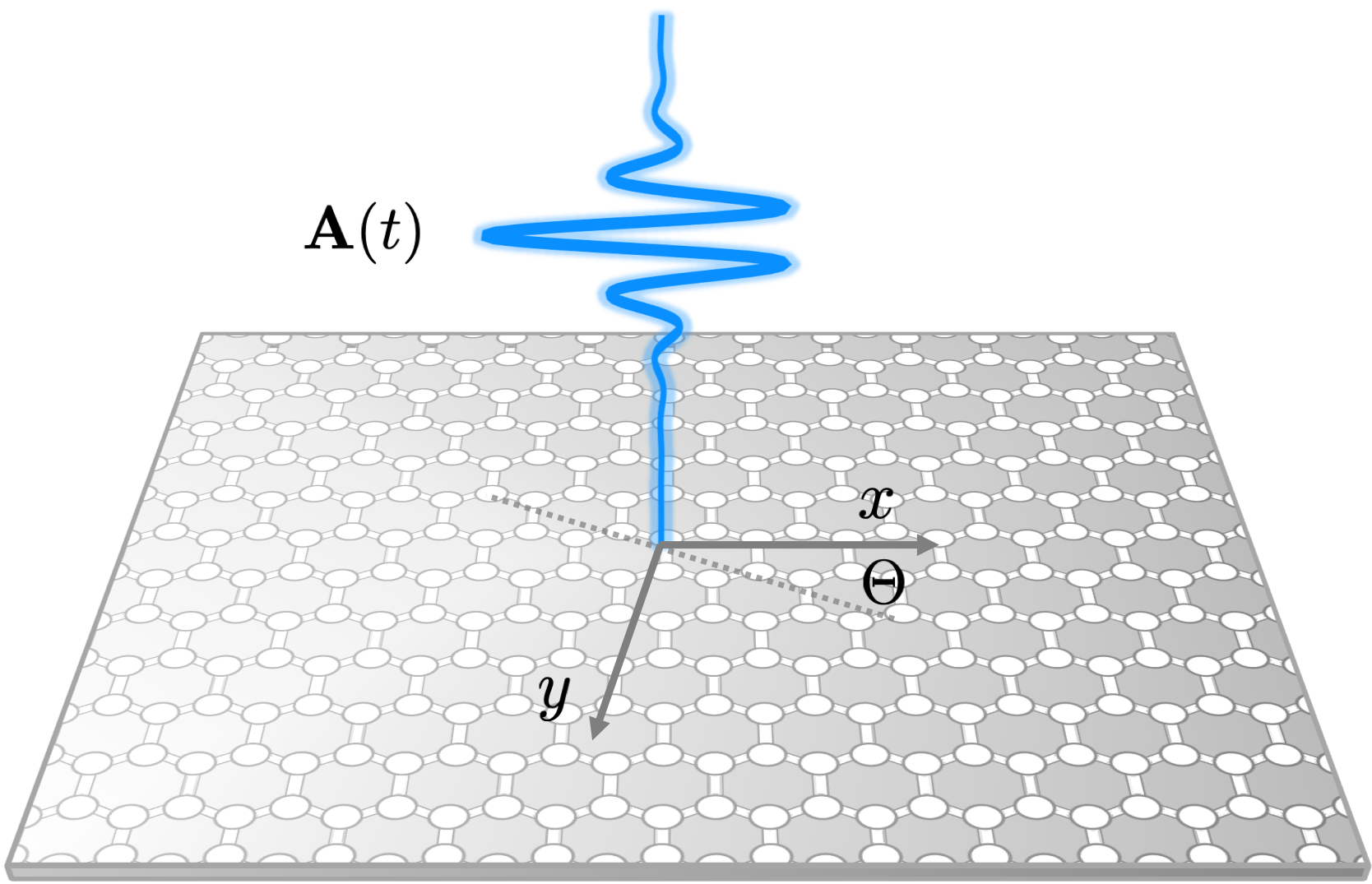
We assume normal incidence conditions, whereby light is assumed to move perpendicularly with respect to the monolayer. In order to study the effects of nonlinear ultrashort light-matter interactions, we choose the velocity gauge, wherein the electromagnetic field couples to the carriers via the minimal substitution: the in-plane carrier momentum $\mathbf{k}=(k_{x},k_{y})\equiv|\mathbf{k}|(\cos\phi_{\mathbf{k}},\sin\phi_{\mathbf{k}})$ is mapped to a time-dependent wavevector $\bm{\pi}_{\mathbf{k}}(t)$, through the assignment $\mathbf{k}\mapsto\bm{\pi}_{\mathbf{k}}(t)\equiv\mathbf{k}+e/(\hbar c)\mathbf{A}(t)$, where $\mathbf{A}(t)$ is the electromagnetic vector potential. We consider linearly polarised light and thus introduce a directional angle $\Theta$, which sets the direction of oscillation of the electric field relative to the monolayer plane. A schematic depiction of the geometry considered may be found in Fig. 2.
Consequently, one has $\textbf{A}(t)=(A_{x}(t),A_{y}(t))\equiv A(t)(\cos\Theta,\sin\Theta)$. The canonical momentum is now split in polars through $\bm{\pi}_{\mathbf{k}}(t)=(\pi_{x}(t),\pi_{y}(t))=|\bm{\pi}_{\mathbf{k}}(t)|(\cos\theta_{\mathbf{k}}(t),\sin\theta_{\mathbf{k}}(t))$, with:

Extrema of bands of the dispersion of a quasiparticle lead to the identification of valleys in momentum space. The goal is to find a suitable Hamiltonian $H^{\xi}_{\mathbf{k}}(t)$ modelling the dynamics of a carrier of wavevector $\mathbf{k}$ in a valley $\xi$, within two effective bands. Any $2$-by-$2$ Hermitian operator may be expanded over the Pauli basis $\{\sigma_{\nu}\penalty\ |\penalty\ \nu=0,1,2,3\}$, where $\sigma_{0}$ is taken as the identity $\mathbb{I}_{2}$ and the remaining respective components as the usual 2D Pauli matrices, i.e. $H_{\mathbf{k}}(t)=\sum_{\nu}a_{\nu,\mathbf{k}}(t)\sigma_{\nu}$. For particular real-valued functions $f_{\mathbf{k}},r_{\mathbf{k}}$ and $g_{\mathbf{k}}$, it can be written in matrix form as:

The newly-introduced phase, termed the warping phase $\nu_{\mathbf{k}}(t)$, appears whenever different hopping contributions (on the off-diagonal entries) rotate at different frequencies. In TMDs, this phase is, perhaps not surprisingly, related to the effect of trigonal warping and this can be seen in Eq. (17c).
Introducing the band index to denote the conduction ($\lambda=+1$) and valence ($\lambda=-1$) bands, the dispersion of each band $\lambda$ is easily obtained through solving $\text{det}[H_{\mathbf{k}}(t)-\epsilon^{\lambda}_{\mathbf{k}}(t)\mathbb{I}]=0$. Note that, due to the optical field, this instantaneous dispersion is also time-dependent and will be written as:

wherein the contributions to the bands asymmetry are lumped in $\epsilon^{a}_{\mathbf{k}}$ and the hopping contributions in $\epsilon^{b}_{\mathbf{k}}$:

For example, and ignoring the optical coupling, gapless graphene has $\epsilon^{a}_{\mathbf{k}}=0$ and $\epsilon^{b}_{\mathbf{k}}=\hbar v_{\rm F}|\mathbf{k}|$ — the usual Dirac cones.
The instantaneous band eigenstates of the full Hamiltonian solve $H_{\mathbf{k}}(t)\ket{u^{\lambda}_{\mathbf{k}}(t)}=\epsilon^{\lambda}_{\mathbf{k}}(t)\ket{u^{\lambda}_{\mathbf{k}}(t)}$ and may be written as:

where instantaneous orthonormality $\braket{u^{\lambda}_{\mathbf{k}}(t)|u^{\lambda^{\prime}}_{\mathbf{k}}(t)}=\delta_{\lambda\lambda^{\prime}}$ was applied. Of further interest, a time-dependent Berry phase $\eta^{\lambda}_{\mathbf{k}}(t)$ may appear in the dynamics of the carriers; its time derivative is $\dot{\eta}^{\lambda}_{\mathbf{k}}(t)\equiv i\braket{u^{\lambda}_{\mathbf{k}}|\dot{u}^{\lambda}_{\mathbf{k}}}=-\xi\lambda z_{\mathbf{k}}(\dot{\theta}_{\mathbf{k}}-\dot{\nu}_{\mathbf{k}})/2$, where $z_{\mathbf{k}}\equiv\left(r_{\mathbf{k}}-\epsilon_{\mathbf{k}}^{a}\right)/\epsilon_{\mathbf{k}}^{b}$. The electric dipole element associated to this two-level system originates from the electron and hole states coupling and is given by:

The existence of a real part in this element implies that the dipole moment contains an imaginary part. For instance, this feature is discussed and its form shown for massive Dirac fermions in Ref. Carvalho et al. 2018, Eq. (11) .

This procedure so far applies to any system for which an effective two-band model is sensible. In order to obtain the specific functions $a_{\nu,\mathbf{k}}$ (and consequently $f_{\mathbf{k}},r_{\mathbf{k}},g_{\mathbf{k}},\nu_{\mathbf{k}}$), which dictate the carrier dynamics across a particular TMD monolayer, approximations are needed. Within the framework of the $\mathbf{k}\cdot\mathbf{p}$ expansion Voon and Willatzen 2009, the Hamiltonian describing the dynamics of the carriers must therefore be expanded up to an adequate order.
Several works, e.g., in Refs. Xiao et al. 2012; Xu et al. 2014, only consider a first-order $\mathbf{k}\cdot\mathbf{p}$ approximation when modelling the electronics of carriers in TMD monolayers, yielding a massive Dirac fermion description. For low-lying electronic states interacting with optical fields of low intensity, this treatment suffices to capture the linear optical properties of the centrosymmetric medium. However, in order to accurately capture nonlinear light-matter phenomena of noncentrosymmetric media across the entire BZ, such expansion is clearly insufficient. Higher-order terms in the $\mathbf{k}\cdot\mathbf{p}$ expansion must be considered so that the centrosymmetry $\mathbf{k}\leftrightarrow-\mathbf{k}$ is explicitly broken. This is a key observation and what allows the present treatment to incorporate higher-order electronic contributions, such as trigonal warping, to the nonlinear contributions to the photo-generated current.
Furthermore, spin dependences are considered by including a first-order contribution originated from spin-orbit coupling (SOC) effects, leading to a valence band shift. Such a procedure leads to the Hamiltonian written as:

Here, $H^{(i)}_{\mathbf{k}}$ are the i^th-order corrections in the $\mathbf{k}\cdot\mathbf{p}$ expansion, whereas $H^{\rm SOC}_{\mathbf{k}}$ is the SOC contribution, acting on $s=+1(-1)\penalty\$ spin up (down) states. Note that in this way, all $4=2$ (on $\xi$) $\times\penalty\ 2$ (on $s$) degrees of freedom are incorporated into one expression. For the orbital configurations of TMDs, the exact functions in Eq. (2) that resulted from the expansion rely on a set of nine phenomenological energy parameters typical of each particular monolayer Liu et al. 2013 – $\gamma_{i}\penalty\ (i=0,...,6)$, $\gamma_{\rm SOC}$ and $\Delta$ – and may be found in Eq. (17). As for the Hamiltonian operators in Eq. (7), both their functional form, written as an expansion over the Pauli basis, and their matrix form may be found in the Appendix in Table 1.
In order to show the trigonal warping in the valence band and electron-hole symmetry, the dispersion of Eq. (3) is plotted in Fig. 3, for both valleys and bands using the parameters of $\tilde{H}^{(3)}_{\mathbf{k}}$ given in Sec. IV.1. The trigonal warping mostly deforms the otherwise-circular Fermi surface on the valence band along the angles $n2\pi/3$, $n\in\mathbb{Z}$, leaving the conduction band nearly isotropic. This is supported by ab-initio calculations Zahid et al. 2013; Kormányos et al. 2013, symmetry analysis Rostami et al. 2013 and experimental evidence Alidoust et al. 2014. Note that the SOC coupling is taken to first-order and therefore not momentum-dependent, leading to a mere shift in the valence bands which cannot be visualised in the figure.

With the knowledge of how to obtain the dynamics of the carriers when coupled to the optical field, we now seek to obtain the surface current $\mathbf{J}(t)=(J_{x}(t),J_{y}(t))$ generated across the sample as a result of such light-matter interactions. To this end, the microscopic contributions of each $\mathbf{k}$ state are obtained first. Due to the $\mathbf{k}\cdot\mathbf{p}$ expansion applied in Eq. (7), and noting that $H^{\rm SOC}_{\mathbf{k}}$ does not contribute to the current as it is not $\mathbf{k}$ dependent, the operator associated to the current density in a Cartesian coordinate $\mu\in\{x,y\}$ may be written as $\hat{j}_{\mu,\mathbf{k}}(t)=\sum_{i}\hat{j}^{(i)}_{\mu,\mathbf{k}}(t)$. A natural definition of each contribution is the so-called paramagnetic current operator

For the wavefunction in Eq. (9), each operator leads to the current:

The first term contains intraband and interband contributions, depending on whether currents originate from the same or opposite bands, respectively. The latter term must be considered in order to regularise the otherwise divergent first term. If the regularisation term is incorporated in the intraband current, the current may be written as:

In this fashion, the current generation is predicted exactly and nonperturbatively by knowing the two-level system dynamics through the DBEs of Eq. (10) as:

For the case of Mo$S_{2}$ monolayers, the exact functional form of these currents for all orders and Cartesian components is rather cumbersome and may be found in Table 2 (intraband) and Table 3 (interband).
Consequently, the current may be estimated once the system in study is well resolved in momentum space i.e. when $a_{\mu,\nu}^{(i)}(\mathbf{k})$ is known. One can see in Eq. (14) that the intraband currents depend on the inversion $w_{\mathbf{k}}$, viz the carrier populations while the interband contributions are dictated by the polarisation $q_{\mathbf{k}}$. Direct calculation of these terms shows that two quantities determine the current composition for either contribution; the ratio $g_{\mathbf{k}}/\epsilon_{\mathbf{k}}^{b}\penalty\ (z_{\mathbf{k}})$ expresses the relative contribution of the hopping (on-site) terms which appear as off-diagonal (diagonal) terms in the Hamiltonian of Eq. (2). These strengths are in fact constrained through $(g_{\mathbf{k}}/\epsilon_{\mathbf{k}}^{b})^{2}+z_{\mathbf{k}}^{2}=1$.
Note that each contribution $j_{\mu,\mathbf{k}}^{(i)}$ should contain in principle all harmonic contributions due to light i.e. only the electronic field is being expanded and not the optical field. Finally, the physical current is retrieved by averaging all microscopic contributions of both valleys and spin states into account. In the continuum limit, it is:

where $d$ is the thickness of the monolayer, $d\mathbf{k}=kdkd\phi$ is the 2-dimensional differential in momentum space. In order to obtain information in the frequency domain, the power spectrum $S(\omega)$ (in dBs) is introduced as:

where $\tilde{\mathbf{J}}(\omega)$ is the Fourier transform of $\mathbf{J}(t)$.

In order to see how the formal introduction of further terms in the $\mathbf{k}\cdot\mathbf{p}$ expansion impact the harmonic generation predicted by the model, we proceed by defining the truncated Hamiltonians containing the cumulative contributions $\tilde{H}_{\mathbf{k}}^{(i)}\equiv\sum_{j=1}^{i}H_{\mathbf{k}}^{(j)}+H_{\mathbf{k}}^{\rm SOC}$. The phenomenological parameters are taken from Liu et al. 2013 where the lattice constant is $a=3.19$ Å and the gap is $\Delta=1.663$ eV; the remaining constants are denoted here by $\mathbf{g}\equiv(g_{i}\penalty\ |\penalty\ i=0,\penalty\ ...,\penalty\ 6)$ and expressed in eV. Physically speaking, $g_{0}$ sets the Fermi velocity $v_{\rm F}\equiv a\gamma_{0}/\hbar$,$\gamma_{1},2,4,5,6$ quantity electron and hole asymmetries in second and third order and $\gamma_{3}$ sets the strength of trigonal warping.
The linear mode $\tilde{H}^{(1)}_{\mathbf{k}}$ has vanishing entries apart from $\gamma_{0}=1.105$ and it may be seen as a suitable electronic model of doped graphene. The quadratic model $\tilde{H}^{(2)}_{\mathbf{k}}$ has ${\bf g}=(1.059,0.055,0.077,-0.123,0,0,0)$ and $\gamma_{\rm SOC}=0$. The cubic model $\tilde{H}^{(3)}_{\mathbf{k}}$ has ${\bf g}=(1.003,0.196,-0.065,-0.248,0.163,-0.094,-0.232)$ and $\gamma_{\rm SOC}=89.6$ meV. Note that each model uses different corresponding parameters.

Due to the linearity of the derivatives, the corrections to the current may be obtained individually by computing the operators in Eq. (11) and applying them to the general wavefunction as prescribed in Eq. (12). Therefore, the explicit effect of the anisotropy may be explicitly inspected in the harmonic generation.
In Fig. 4, the absolute value of the full current defined in Eq. (15), whose integrand is explicitly given in Table 2 - 3, is shown in Fig. 4(a) for the three $\mathbf{k}\cdot\mathbf{p}$ Hamiltonians $\tilde{H}^{(i)}_{\mathbf{k}},\penalty\ i=1,2,3$. It can be seen that the current roughly follows the pulse profile in time domain. However, both the frequency and amplitude modulation of the signal deviate from each other once the optical field is maximal (the pulse peak is centred about $t=0$) as higher $\mathbf{k}\cdot\mathbf{p}$ terms are included. We shall focus on the total, physically-relevant current, which is composed of both intraband and interband contributions. However, we remark that, given the resonant pumping conditions, the interband contributions dominate over their intraband counterparts, although the intraband current amplitude increases for higher $\mathbf{k}\cdot\mathbf{p}$ models, contrary to the amplitude suppression shown in Fig. 4(a).

The effects of this modulation may be seen in the harmonic composition of the currents in Fig. 4(b), where the power spectrum of Eq. (16) is plotted in units of the pulse-normalised frequency $\omega/\omega_{0}$. The linear model shows the well-known strong third harmonic observed in graphene, as well as small second-harmonic peaks previously reported to exist due to light-induced dynamical centrosymmetry breaking Carvalho et al. 2017; Carvalho et al. 2018. As expected, the explicit centrosymmetry breaking of the lattice arrangement as depicted in Fig. 1 induces strong even harmonics, which are observed once quadratic and cubic terms are added. Linked to second harmonic generation, optical rectification can also be seen to increase in the same fashion in the DC limit (at $\omega=0$). This turns out to be an interband-driven process.

We close this subsection with a due remark. The output current $\mathbf{J}$ has, perhaps surprisingly, both non-vanishing longitudinal and transverse components to the electric field, polarised along $\Theta$. The present machinery has been previously applied to both gapless and gapped graphene monolayers in Carvalho et al. 2017; Carvalho et al. 2018. The gapless case presented a straightforward analysis: only current along the same direction as the electric field was found upon integration in Eq. (15), where a degeneracy factor $g_{v}=2$ was verified. Once the system became gapped, the transverse current still vanished, but now due to a cancellation of valley transverse currents. With the introduction of further $\mathbf{k}\cdot\mathbf{p}$ terms, this no longer holds. To verify the invariance of this result, we applied a rotation $\mathcal{R}(\alpha)$ to the basis $\{\hat{x},\hat{y}\}$ and checked if $\mathcal{R}(\alpha)\mathbf{J}(t)$ admits only one non-vanishing component. No angle was found to yield this result, leading us to conclude these corrections to the dispersion may indeed create transverse currents.

Given the anisotropy properties of the dispersion shown in shown in Fig.1, it is expected that the photo-generated current across the sample depends on the relative angle between the lattice orientation and the oscillation of the electric field. This the polarisation angle $\Theta$ is measured on the sample plane and depicted in Fig.2. In order to appreciate such dependence, a MoS₂ monolayer is excited using the phenomenological energy parameters of $\tilde{H}^{(3)}_{\mathbf{k}}$ in resonance conditions i.e. with $\Delta=2\hbar\omega_{0}$, when sweeping through the range $0\leq\Theta\leq\pi$. For each angle, the momentum-integrated spectrum of Eq. (16) is calculated and the maximum intensity of each harmonic peak is recorded. Such plot is shown in Fig.5 for second (SHG) and third harmonic (THG)-generated peaks. To help visualise the trend, a polynomial fit is added to each harmonic.

To relate the anisotropy to the polarisation modulation, dashed lines of strong trigonal warping are added increasingly at $\Theta=\pi/3,\pi/6,\pi/2,2\pi/3$ and $5\pi/6$. The SHG signal shows a consistent modulation, maxima at $\Theta\approx n\pi/3$ and minima at $\Theta\approx(2n+1)\pi/6$, leading to the same period of the trigonal warping, of $\pi/3$. The THG modulation shows somewhat similar patterns as SHG but differs at small angles, showing a very large variation (note the scale is logarithmic). Higher harmonic peaks show more complex, nontrivial modulation. Their exact functional form is not instructive for our study since, as the harmonic order increases, the efficiency of nonlinear optical processes decays exponentially and are therefore not shown.
Here, we focus on the possibility of harmonic crossovers i.e. higher, less efficient harmonics amplitudes to overcome lower, more efficient harmonics. Since harmonics of all parity may be created in the present cubic model, as demonstrated in Fig. 4(b), this possibility is tested. Indeed, a crossover range where the third-harmonic is stronger than the second-harmonic is found, namely between $\pi/6\leq\Theta_{\rm c}\leq 5\pi/6$. This difference is about 4 orders of magnitude, meaning that it could potentially be measured in experimental conditions.

References

- Kolobov and Tominaga (2016) A. V. Kolobov and J. Tominaga, Two-Dimensional Transition-Metal Dichalcogenides, Vol. 239 (Springer, 2016).
- Singh et al. (2018) A. K. Singh, P. Kumar, D. Late, A. Kumar, S. Patel, and J. Singh, Applied Materials Today 13, 242 (2018).
- Kormányos et al. (2013) A. Kormányos, V. Zólyomi, N. D. Drummond, P. Rakyta, G. Burkard, and V. I. Fal’ko, Phys. Rev. B 88, 045416 (2013).
- Säynätjoki et al. (2017) A. Säynätjoki, L. Karvonen, H. Rostami, A. Autere, S. Mehravar, A. Lombardo, R. A. Norwood, T. Hasan, N. Peyghambarian, H. Lipsanen, et al., Nature communications 8, 893 (2017).
- Zhu et al. (2011) Z. Y. Zhu, Y. C. Cheng, and U. Schwingenschlögl, Phys. Rev. B 84, 153402 (2011).
- Schaibley et al. (2016) J. R. Schaibley, H. Yu, G. Clark, P. Rivera, J. S. Ross, K. L. Seyler, W. Yao, and X. Xu, Nature Reviews Materials 1 (2016), 2016/08/23/online.
- Xu et al. (2014) X. Xu, W. Yao, D. Xiao, and T. F. Heinz, Nature Physics 10, 343–350 (2014).
- Xiao et al. (2012) D. Xiao, G.-B. Liu, W. Feng, X. Xu, and W. Yao, Physical Review Letters 108, 196802 (2012).
- Zheng et al. (2018) W. Zheng, Y. Jiang, X. Hu, H. Li, Z. Zeng, X. Wang, and A. Pan, Advanced Optical Materials , 1800420 (2018).
- Liu et al. (2016) H. Liu, Y. Li, Y. S. You, S. Ghimire, T. F. Heinz, and D. A. Reis, Nature Physics (2016).
- Yu et al. (2014) H. Yu, G.-B. Liu, P. Gong, X. Xu, and W. Yao, Nature communications 5 (2014).
- Autere et al. (2018) A. Autere, H. Jussila, A. Marini, J. R. M. Saavedra, Y. Dai, A. Säynätjoki, L. Karvonen, H. Yang, B. Amirsolaimani, R. A. Norwood, N. Peyghambarian, H. Lipsanen, K. Kieu, F. J. G. de Abajo, and Z. Sun, Phys. Rev. B 98, 115426 (2018).
- Khorasani (2018) S. Khorasani, Communications in Theoretical Physics 70, 344 (2018).
- Wang et al. (2018) Y. Wang, Z. Guo, J. You, Z. Zhang, X. Zheng, and X. Cheng, Photonic Sensors , 1 (2018).
- Xia et al. (2014) F. Xia, H. Wang, D. Xiao, M. Dubey, and A. Ramasubramaniam, Nature Photonics 8, 899 (2014).
- Gmitra et al. (2016) M. Gmitra, D. Kochan, P. Högl, and J. Fabian, Physical Review B 93, 155104 (2016).
- Liu et al. (2013) G.-B. Liu, W.-Y. Shan, Y. Yao, W. Yao, and D. Xiao, Physical Review B 88, 085433 (2013).
- Rostami et al. (2013) H. Rostami, A. G. Moghaddam, and R. Asgari, Physical Review B 88, 085440 (2013).
- Carvalho et al. (2018) D. N. Carvalho, F. Biancalana, and A. Marini, Physical Review B 97, 195123 (2018).
- Voon and Willatzen (2009) L. C. L. Y. Voon and M. Willatzen, The kp method: electronic properties of semiconductors (Springer Science & Business Media, 2009).
- Zahid et al. (2013) F. Zahid, L. Liu, Y. Zhu, J. Wang, and H. Guo, Aip Advances 3, 052111 (2013).
- Alidoust et al. (2014) N. Alidoust, G. Bian, S.-Y. Xu, R. Sankar, M. Neupane, C. Liu, I. Belopolski, D.-X. Qu, J. D. Denlinger, F.-C. Chou, et al., Nature communications 5, 1 (2014).
- Ishikawa (2010) K. L. Ishikawa, Physical Review B 82, 201402 (2010).
- Carvalho et al. (2017) D. N. Carvalho, A. Marini, and F. Biancalana, Annals of Physics 378, 24 (2017).
- McCann and Koshino (2013) E. McCann and M. Koshino, Reports on Progress in Physics 76, 056503 (2013).
- Liu et al. (2010) C.-X. Liu, X.-L. Qi, H. Zhang, X. Dai, Z. Fang, and S.-C. Zhang, Physical Review B 82, 045122 (2010).
- Villari et al. (2018) L. D. M. Villari, I. Galbraith, and F. Biancalana, Phys. Rev. B 98, 205402 (2018).
- Van’t Erve et al. (2016) O. M. Van’t Erve, A. T. Hanbicki, A. L. Friedman, K. M. McCreary, E. Cobas, C. H. Li, J. T. Robinson, and B. T. Jonker, Journal of Materials Research 31, 845 (2016).
- Dey et al. (2016) P. Dey, J. Paul, Z. Wang, C. Stevens, C. Liu, A. Romero, J. Shan, D. Hilton, and D. Karaiskaj, Physical review letters 116, 127402 (2016).
- Mak and Shan (2016) K. F. Mak and J. Shan, Nature Photonics 10, 216 (2016).
- Wang (2013) Z. M. Wang, MoS2: materials, physics, and devices, Vol. 21 (Springer Science & Business Media, 2013).