Skier and loop-the-loop with friction

Two classic homework exercises in an elementary mechanics course are the skier on a hemispherical hill (Fig. 1) and the particle on a loop-the-loop track (Fig. 2).mechanics_books Both problems illustrate nicely the use of conservation of energy (to find the speed as a function of height) followed by ${\bf F}=m{\bf a}$ (to find the normal force).

It is interesting to consider what happens when the hill or track is endowed with a coefficient of kinetic friction $\mu$. Somewhat surprisingly, the exact differential equations turn out to be analytically solvable.Franklin_80; Mania_02; Mungan_03; Hite_04; Prior_07; DeLange_08; Klobus_11; Nahin_15; Gonzalez-Cataldo_17; DelPino_18 Our purpose here is to provide a unified treatment of the two problems, using only elementary methods that are easily accessible to undergraduates (e.g. linear first-order differential equations). Though most of our results have been obtained previously — as we shall document in detail — they are somewhat scattered in the literature. It may thus be of some modest value to have a complete elementary derivation collected in one place.

The skier and loop-the-loop problems give rise to very similar differential equations, which differ only by some sign changes. However, these sign changes lead to significant differences in the qualitative interpretation of the solutions. Since the skier problem turns out to be somewhat simpler, we treat it first and give a complete solution; in particular, we determine the exact “phase diagram” in the two-dimensional parameter plane. For the loop-the-loop, we solve the differential equations only up to the first time (if any) that the particle halts or completes one cycle of the loop, so we obtain only a partial “phase diagram”. The full phase diagram will (as we explain later) contain an infinite sequence of bifurcations, and we leave its computation to a reader who wishes to take up where we have left off.

Consider a skier of mass $m$ on a hemispherical hill of radius $R$ (or more generally, any hill of circular cross section) and coefficient of kinetic friction $\mu$, entering at the top with forward velocity $v_{0}$; let $\theta$ denote the angle from the vertical (Fig. 1). Then the radial and tangential components of ${\bf F}=m{\bf a}$ areF=ma

This is a pair of coupled differential equations for the unknown functions $\theta(t)$ and $N(t)$. We stress, however, that these equations are valid only as long as $N\geq 0$; after that, the skier flies off the hill. Since it is clear that the skier will only go down the hill, not up, we have $\dot{\theta}\geq 0$ throughout the motion, and the factor $\mathop{\rm sgn}\nolimits(\dot{\theta})$ in Eq. (2) can be dropped.note_static_friction

Differentiating Eq. (1) with respect to time yields

and inserting $\ddot{\theta}$ from Eq. (2) [with $\mathop{\rm sgn}\nolimits(\dot{\theta})=1$] yields

Using the chain rule $dN/dt=(dN/d\theta)(d\theta/dt)$ we can eliminate $\dot{\theta}$ from Eq. (4), leading to

This is a first-order inhomogeneous linear differential equation with constant coefficients for the unknown function $N(\theta)$, and it can be solved by the method of integrating factors. Here the integrating factor is $e^{-2\mu\theta}$, and the solution isalternate_solution

where $N_{0}=N(0)$. We again stress that this solution is valid only where $N(\theta)\geq 0$; at the first angle (if any) where $N(\theta)$ crosses zero to a negative value, the skier flies off the hill.

Evaluating Eq. (1) at $\theta=0$, where the skier’s angular velocity is $\dot{\theta}=v_{0}/R$, we obtain $N_{0}=mg-mv_{0}^{2}/R$. In particular, if the dimensionless parameter $\lambda\stackrel{{\scriptstyle\rm def}}{{=}}v_{0}^{2}/gR$ is $\geq 1$, then $N_{0}\leq 0$ and the skier immediately flies off the hill; we therefore assume henceforth that $0\leq\lambda<1$. Inserting $N_{0}=(1-\lambda)mg$ in Eq. (6), we obtain

which is the closed-form solution giving the normal force as a function of angle.

In the absence of friction ($\mu=0$), Eq. (7) simplifies to

This is a decreasing function of $\theta$, and skier flies off the hill when $N=0$, i.e. when

In the usual textbook problem one has also $v_{0}=0$ (i.e. $\lambda=0$), and we obtain the standard answer that the skier flies off at angle $\theta=\cos^{-1}(2/3)\approx 48.19^{\circ}$.

When $\mu>0$, by contrast, the normal force is no longer a decreasing function of $\theta$, nor is it guaranteed to reach zero within the interval $0\leq\theta\leq\pi/2$. Indeed, $dN/d\theta|_{\theta=0}=2\mu(1-\lambda)mg>0$, so the normal force is initially increasing.

We can also obtain the velocity as a function of angle. It is convenient to define the dimensionless quantity $\Lambda\stackrel{{\scriptstyle\rm def}}{{=}}v^{2}/gR=R\dot{\theta}^{2}/g$; its value at $\theta=0$ is what we have called $\lambda$. Then from Eq. (1) we have immediately

[which reduces to $N_{0}=(1-\lambda)mg$ when $\theta=0$] or equivalently

In particular, from $N\geq 0$ we deduce that $\Lambda\leq\cos\theta$: this gives the maximum speed that the skier can have at any given angle if she is to avoid flying off the hill. Combining Eqs. (7) and (11) gives the closed-form solution for the speed as a function of angle:speed_as_a_function_of_angle

Note, however, that this solution is valid only where $\Lambda(\theta)\geq 0$; at the first angle (if any) where $\Lambda(\theta)=0$, the skier comes to rest (perhaps only asymptotically as $t\to+\infty$). The solution (12) must therefore be supplemented by the two inequalities $0\leq\Lambda(\theta)\leq\cos\theta$.

From Eqs. (5) and (10)/(11) we see that $\Lambda(\theta)$ satisfies the differential equationdifferential_equation

The solution of this differential equation with the initial condition $\Lambda(0)=\lambda$ is of course Eq. (12).alternate_solution

In the absence of friction ($\mu=0$), Eq. (12) simplifies to

which is just the expression for conservation of energy: ${1\over 2}mv^{2}={1\over 2}mv_{0}^{2}+mgR(1-\cos\theta)$. More generally, the kinetic energy plus gravitational potential energy is

so that

The work-energy theorem asserts that $dE/dt$ must equal the rate of work done by friction, which is $-\mu NR\dot{\theta}$; and this equality is an immediate consequence of Eqs. (10), (13) and (16). Conversely, the differential equation (13) could alternatively be derived by combining the work-energy theorem with Eqs. (10) and (16).work-energy It may be useful for students to compare these two derivations: one directly from the Newtonian equations of motion, the other from the work-energy theorem.

Finally, we can use Eq. (12) to obtain the time-dependence of the motion. From $\Lambda=R\dot{\theta}^{2}/g$ we have

and hence

We can now analyze the qualitative behavior of the motion as a function of the two parameters $\mu\in[0,\infty)$ and $\lambda\in[0,1)$. We have seen that the skier halts when $\Lambda(\theta)=0$, or flies off the hill when $\Lambda(\theta)=\cos\theta$, whichever happens first; if neither happens for $\theta<\pi/2$, then the skier reaches the bottom of the hill. (We will see later that this last case never occurs.) The critical solution that separates these two scenarios is given by the trajectory for which the skier halts at an angle $\theta_{\star}$ (hence $\Lambda(\theta_{\star})=0$) that also satisfies $\Lambda^{\prime}(\theta_{\star})=0$: see the curve marked $\lambda=\lambda_{\star}$ in Fig. 3. Applying this condition in Eq. (13) leads immediately toref_thetastar

Substituting this in Eq. (12), we obtain the relationship between the initial velocity and the friction coefficient that defines the phase boundary:lambdastar_mu

Please observe that $\lambda_{\star}(\mu)$ is an increasing function of $\mu$ that runs from 0 to 1 as $\mu$ runs from 0 to $\infty$ (see Fig. 4).

In this way we have obtained a “phase diagram” that divides the $(\mu,\lambda)$ plane into three possible qualitative behaviors:

• •

  For $0\leq\lambda<\lambda_{\star}(\mu)$, the skier halts after a finite time at some angle $\theta_{\rm halt}(\mu,\lambda)$: this angle is an increasing function of $\lambda$ that runs from 0 to $\arctan\mu$ as $\lambda$ runs from 0 to $\lambda_{\star}(\mu)$.

• •

  For $\lambda=\lambda_{\star}(\mu)$, the skier comes to rest asymptotically as $t\to+\infty$ at the angle $\theta=\arctan\mu$.note_equilibrium

• •

  For $\lambda_{\star}(\mu)<\lambda<1$, the skier flies off the hill at some angle $\theta_{\rm fly}(\mu,\lambda)$: this angle is a decreasing function of $\lambda$ that tends to 0 as $\lambda\to 1$.

The curve $\lambda_{\star}(\mu)$ thus forms the boundary between the “halt” phase and the “fly-off” phase (see again Fig. 4).phase_diagram In particular, the skier always either halts or flies off; she never reaches angle $\pi/2$.

Some typical curves of $\Lambda(\theta)$ for all three scenarios are shown in Fig. 3. Note in particular that $\Lambda(\theta)=\Lambda^{\prime}(\theta)=0$ when $\lambda=\lambda_{\star}(\mu)$ and $\theta=\theta_{\star}(\mu)$; and note the fundamental qualitative difference between the curves for $\lambda<\lambda_{\star}(\mu)$, which reach the $\Lambda=0$ axis, and those for $\lambda>\lambda_{\star}(\mu)$, which do not.refs_for_fig.Lambda.theta

Some typical curves of $\theta_{\rm halt}(\mu,\lambda)$ as a function of $\lambda$ are shown in Fig. 5, and some typical curves of $\theta_{\rm fly}(\mu,\lambda)$ as a function of $\lambda$ are shown in Fig. 6. Please note the discontinuous change in behavior as the phase boundary $\lambda_{\star}(\mu)$ is crossed: $\theta_{\rm fly}(\mu,\lambda_{\star}(\mu))$ [the dotted curve in Fig. 6] is much larger than $\theta_{\rm halt}(\mu,\lambda_{\star}(\mu))$ [the dashed curve in Fig. 5].ref_for_figs_thetahalt+thetafly This is a very simple example of sensitive dependence to initial conditions, giving rise to a discontinuous phase transition — a phenomenon pointed out already by James Clerk Maxwell in 1876.ref_Maxwell

Since the proofs of all the previous claims involve some slightly intricate calculus, we relegate them to Appendix A in the Supplementary Materials.ref_supplementary

Let us remark, finally, that by the same methods one can study the more general problem in which the coefficient of kinetic friction is an arbitrary function $\mu(\theta)$ of the position along the hill: the equation (5) is still a first-order inhomogeneous linear differential equation for the unknown function $N(\theta)$ — albeit now one with nonconstant coefficients — so can still be solved by the method of integrating factors (though the result may not be analytically expressible in terms of elementary functions). We leave it to interested readers to pursue this generalization.

Some recent related articles are Refs. Gonzalez-Cataldo_17, DelPino_18 and Ivchenko_21, which study a particle sliding down an arbitrary curve in the presence of kinetic friction; Ref. Balart_19, which uses the Lagrangian formalism with Lagrange multipliers to analyze a particle sliding without friction down an arbitrary concave curve; and Ref. Mejia_20, which studies a ball rolling (initially without slipping, later with sliding and kinetic friction) on an arbitrary curve in the presence of gravity, including an experimental realization.

A block of mass $m$ is injected with forward velocity $v_{0}$ into a loop-the-loop track of radius $R$ and coefficient of kinetic friction $\mu$; let $\theta$ denote the angle up from the bottom, as shown in Fig. 2. (In one common version of the problemmechanics_books, the block is released from rest at height $h$ and slides to the bottom via a frictionless track; in this case $v_{0}=\sqrt{2gh}$.) The radial and tangential components of ${\bf F}=m{\bf a}$ are

As before, these equations are valid only as long as $N\geq 0$; after that, the block falls off the track.

The loop-the-loop problem is more complicated than the skier, for three reasons: the particle can cycle around the track; it can reverse direction; and it can halt due to static friction. Each time the particle reverses direction, we need to apply Eq. (22) with a new value for $\mathop{\rm sgn}\nolimits(\dot{\theta})$; this repeated switching between different equations seems quite complicated, and probably needs to be handled by numerical solution.loop-the-loop_reverses To simplify matters, we will here follow the block only until it first reaches $\dot{\theta}=0$ or falls off the track; we therefore have $\dot{\theta}\geq 0$.

Proceeding as in Eqs. (3)–(5) leads to the differential equation

for the unknown function $N(\theta)$; this equation differs from Eq. (5) only by the replacement $\mu\to-\mu$. The solution is therefore

where $N_{0}=N(0)$. Applying Eq. (21) at $\theta=0$, where the block’s angular velocity is $\dot{\theta}=v_{0}/R$, we see that $N_{0}=mg+mv_{0}^{2}/R$. Using again the dimensionless parameter $\lambda\stackrel{{\scriptstyle\rm def}}{{=}}v_{0}^{2}/gR$, we have $N_{0}=(1+\lambda)mg$ and hence

To obtain the velocity as a function of angle, we define once again the dimensionless quantity $\Lambda\stackrel{{\scriptstyle\rm def}}{{=}}v^{2}/gR=R\dot{\theta}^{2}/g$, which takes the value $\lambda$ at $\theta=0$. Then from Eq. (21) we have

[which reduces to $N_{0}=(1+\lambda)mg$ when $\theta=0$] and thereforeloop-the-loop_Lambda_theta

Since $\Lambda\geq 0$, we must have $N\geq mg\cos\theta$; and when $N=mg\cos\theta$, the block comes instantaneously to rest. After that, the particle might either reverse direction or halt due to static friction. As mentioned earlier, we refrain from following the particle beyond the first time it comes instantaneously to rest.

The solution (25) must therefore be supplemented by the two inequalities $N(\theta)\geq 0$ and $N(\theta)\geq mg\cos\theta$. (Please note that, unlike in the skier problem, both of these inequalities point in the same direction; this radically changes the nature of the qualitative analysis.) The block comes instantaneously to rest when $N(\theta)=mg\cos\theta$, or falls off the track when $N(\theta)=0$, whichever happens first; if neither happens for $\theta<2\pi$, then the block completes one full cycle of the loop-the-loop. Now, the inequality $N(\theta)\geq mg\cos\theta$ is the more stringent one in the lower half of the loop-the-loop (that is, $-\pi/2\leq\theta\leq\pi/2$ modulo $2\pi$), while the inequality $N(\theta)\geq 0$ is the more stringent one in the upper half of the loop-the-loop (that is, $\pi/2\leq\theta\leq 3\pi/2$ modulo $2\pi$). Therefore, the block can come instantaneously to rest only in the lower half of the loop-the-loop, and it can fall off the track only in the upper half of the loop-the-loop.

In the absence of friction ($\mu=0$), Eq. (25) simplifies to

If $\lambda\leq 2$, then the block reverses direction at

(a value that follows immediately from conservation of energy) and oscillates forever between $-\theta_{\rm max}$ and $\theta_{\rm max}$; if $2<\lambda<5$, then the block falls off the track at

which lies between $\pi/2$ and $\pi$; if $\lambda=5$, then the block asymptotically approaches $\theta=\pi$ as $t\to+\infty$; if $\lambda>5$, then the block cycles forever around the track without loss of energy.

In the presence of friction ($\mu>0$), the analysis proceeds as follows:

1) The first step is to determine the conditions under which the particle halts in the first quadrant ($0\leq\theta\leq\pi/2$). The particle halts at angle $\theta$ when $\Lambda(\theta)=0$, i.e. in case the initial velocity satisfies

Since

$\lambda_{\rm halt}(\theta,\mu)$ is an increasing function of $\theta$ in the interval $0\leq\theta\leq\pi/2$ (as is intuitively clear: to reach a larger angle, more initial velocity is needed). In particular, the particle reaches $\theta=\pi/2$ with $\dot{\theta}>0$ if and only if

2) If the particle reaches angle $\pi/2$ without halting, the next step is to determine the conditions under which the particle flies off in the second or third quadrant ($\pi/2\leq\theta\leq 3\pi/2$). The particle flies off at angle $\theta$ when $N(\theta)=0$, i.e. in case the initial velocity satisfies

Note that $\lambda_{\rm fly}(\pi/2,\mu)=\lambda_{\rm halt}(\pi/2,\mu)$. Since

we see that $\lambda_{\rm halt}(\theta,\mu)$ is an increasing function of $\theta$ in the interval from $\pi/2$ to $\pi$, and then a decreasing function in the interval from $\pi$ to $3\pi/2$. The first of these facts is again intuitively clear: to survive to a larger angle without flying off, more initial velocity is needed. The second fact implies that if the particle reaches angle $\pi$ without flying off — that is, if

— then it also reaches angle $3\pi/2$ without flying off. This is intuitively clear when there is no friction, but not so obvious in the presence of friction. This implies — analogously to what happens in the skier problem — a discontinuous change of behavior as $\lambda$ passes through $\lambda_{\rm fly}(\pi,\mu)$. See Fig. 7 for plots of $\lambda_{\rm halt}(\theta,\mu)$ and $\lambda_{\rm fly}(\theta,\mu)$ versus $\theta$ for some selected values of $\mu$.

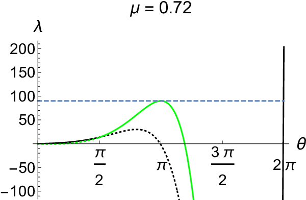3) If the particle reaches angle $\pi$ (and hence also angle $3\pi/2$) without halting or flying off, the next step is to determine what happens in the fourth quadrant ($3\pi/2<\theta<2\pi$). The particle halts at angle $\theta$ in case $\lambda$ equals the quantity $\lambda_{\rm halt}(\theta,\mu)$ defined in Eq. (31). From Eq. (32) we see that $\partial\lambda_{\rm halt}(\theta,\mu)/\partial\theta$ is negative at $\theta=3\pi/2$ and positive at $\theta=2\pi$, with a unique zero at $\theta=2\pi-\arctan\mu$. So $\lambda_{\rm halt}(\theta,\mu)$ is decreasing in the interval $3\pi/2\leq\theta\leq 2\pi-\arctan\mu$ and increasing in the interval $2\pi-\arctan\mu\leq\theta\leq 2\pi$. Its maximum value in the interval $[3\pi/2,2\pi]$ therefore lies either at $\theta=3\pi/2$ or at $\theta=2\pi$. Since we are in the situation $\lambda\geq\lambda_{\rm fly}(\pi,\mu)>\lambda_{\rm fly}(3\pi/2,\mu)=\lambda_{\rm halt}(3\pi/2,\mu)$, the only relevant question is whether $\lambda$ is larger than $\lambda_{\rm halt}(2\pi,\mu)$ or not. If it is, then the particle reaches angle $2\pi$ without halting. If it is not, then the particle halts at some angle in the interval $(2\pi-\arctan\mu,2\pi]$, namely, the unique angle where $\lambda=\lambda_{\rm halt}(\theta,\mu)$. The first of these cases always occurs when $\lambda_{\rm fly}(\pi,\mu)>\lambda_{\rm halt}(2\pi,\mu)$, i.e. when $0\leq\mu<\mu_{\rm crit}\approx 0.713089$. (See Appendix B in the Supplementary Materialsref_supplementary for the proof that there is a unique such value $\mu_{\rm crit}$.) When $\mu\geq\mu_{\rm crit}$, then there is a “halt in fourth quadrant” phase at $\lambda_{\rm fly}(\pi,\mu)\leq\lambda\leq\lambda_{\rm halt}(2\pi,\mu)$ and a “survive to angle $2\pi$” phase at $\lambda\geq\lambda_{\rm halt}(2\pi,\mu)$. We record the formula

4) If the particle survives to angle $2\pi$, then it has there a forward velocity corresponding to a value

Since $\lambda_{\rm halt}(2\pi,\mu)>0$ in the “survive to angle $2\pi$” phase, we have $\lambda_{\rm new}<e^{-4\pi\mu}\lambda$: thus the kinetic energy is reduced by at least a factor $e^{-4\pi\mu}$ at each revolution. The subsequent motion can then be found by repeating the foregoing analysis with $\lambda$ replaced by $\lambda_{\rm new}$.

The resulting phase diagram is shown in Fig. 8. Since $\lambda_{\rm halt}(2\pi,\mu)$ grows extremely rapidly with $\mu$, we have used $\sqrt{\lambda}$ instead of $\lambda$ on the vertical axis, to compress the plot. This phase diagram agrees with the one found by Kłobus (Ref. Klobus_11, Fig. 2); the value of $\lambda_{\rm halt}(2\pi,1)$ also agrees with his. All three phase boundaries are increasing functions of $\mu$: see Appendices B1–B3 in the Supplementary Materials.ref_supplementary

Of course, this phase diagram only follows the particle up to the first time that it reaches $\dot{\theta}=0$ or $\theta=2\pi$. A more complete analysis would show that the phase “survives to angle $2\pi$” is itself divided into sub-phases “halts in the first quadrant” ($2\pi<\theta<5\pi/2$), “flies off the second quadrant” ($5\pi/2<\theta<3\pi$), “halts in the fourth quadrant” ($7\pi/2<\theta<4\pi$) and “survives to angle $4\pi$”; and this latter phase is further divided into sub-phases; and so on infinitely. We leave it to interested readers to work out the details of this infinite sequence of bifurcations.

We are extremely grateful to three referees for their detailed and helpful comments on several versions of this paper.

References

- (1) See e.g. D. Kleppner and R. Kolenkow, An Introduction to Mechanics, 2nd ed. (Cambridge University Press, Cambridge, 2014), Problems 5.1 (loop-the-loop) and 5.6 (block sliding down a sphere); D. Morin, Introduction to Classical Mechanics (Cambridge University Press, New York, 2008), Exercises 5.39 (loop-the-loop) and 5.53 (skier on a frictionless hemisphere of finite mass , which is considerably more difficult than the usual case ).
- (2) L.P. Franklin and P.I. Kimmel, “Dynamics of circular motion with friction,” Amer. J. Phys. 48, 207–210 (1980).
- (3) A.J. Mania, A.W. Mol and C.S.S. Brandão, “Sliding block on a semicircular track with friction,” Revista Brasileira de Ensino de Física 24, 312–316 (2002).
- (4) C.E. Mungan, “Sliding on the surface of a rough sphere,” Phys. Teacher 41, 326–328 (2003).
- (5) G.E. Hite, “The sled race,” Amer. J. Phys. 72, 1055–1058 (2004).
- (6) T. Prior and E.J. Mele, “A block slipping on a sphere with friction: Exact and perturbative solutions,” Amer. J. Phys. 75, 423–426 (2007).
- (7) O.L. de Lange, J. Pierrus, T. Prior and E.J. Mele, “Comment on ‘A block slipping on a sphere with friction: Exact and perturbative solutions’,” Amer. J. Phys. 76, 92–93 (2008).
- (8) W. Kłobus, “Motion on a vertical loop with friction,” Amer. J. Phys. 79, 913–918 (2011).
- (9) P.J. Nahin, Inside Interesting Integrals (Springer, New York, 2015), pp. 112–114.
- (10) F. González-Cataldo, G. Gutiérrez and J.M. Yáñez, “Sliding down an arbitrary curve in the presence of friction,” Amer. J. Phys. 85, 108–114 (2017). Extended version available at https://arxiv.org/abs/1512.00515
- (11) L.A. del Pino and S. Curilef, “Comment on ‘Sliding down an arbitrary curve in the presence of friction’,” Amer. J. Phys. 86, 470–471 (2018).
- (12) See Ref. Mungan_03, Eqs. (1) and (3). See also Ref. Gonzalez-Cataldo_17 for a generalization to an arbitrary curve in the vertical plane, using the Frenet–Serret formalism.
- (13) Taking literally the equations (1)/(2), the skier would reverse direction when and begin climbing back up the hill. But this is not, of course, what actually happens. Rather, when the skier halts, static friction takes over, and the skier remains forever at rest; this occurs because static friction is governed by the inequality , not the equality .
- (14) See also Ref. Mungan_03, Appendix A for an alternate approach to solving Eqs. (5) and (13), which does not require the student to be familiar with the method of integrating factors.
- (15) See Ref. Mungan_03, Eq. (A3); Ref. Prior_07, Eq. (25); Ref. DeLange_08, Eq. (2); Ref. Gonzalez-Cataldo_17, Eq. (23), or Eq. (24) in the arXiv version.
- (16) See Ref. Mungan_03, Eq. (5); Ref. Prior_07, Eq. (17); and Ref. DeLange_08, Eq. (1). See also Ref. Gonzalez-Cataldo_17, Eq. (9) for a generalization to an arbitrary curve in the vertical plane.
- (17) This approach is taken, for instance, in Ref. Prior_07, Eqs.(9) and (17); in Ref. DeLange_08, Eq. (1); and in Ref. DelPino_18 for an arbitrary curve in the vertical plane.
- (18) See Ref. DeLange_08; Ref. Gonzalez-Cataldo_17 (arXiv version), Eq. (59) ff.
- (19) See Ref. DeLange_08, Eq. (5); Ref. Gonzalez-Cataldo_17 (arXiv version), Eq. (62). This latter paper also gives analogous formulae for the parabola, cycloid, catenary and ellipse.
- (20) It can be seen directly from the equations of motion (1)/(2) that this “asymptotic equilibrium” position can only be . To see this, observe that for all , and that as . Combining Eqs. (1)/(2) as then yields and . This argument does not apply to the “subcritical” trajectories in which the skier halts after a finite time, since in these trajectories but at the halting time.
- (21) See Ref. DeLange_08, Fig. 1; Ref. Gonzalez-Cataldo_17 (arXiv version), Fig. 13. This latter figure also shows the phase diagram for the parabola, cycloid, catenary and ellipse.
- (22) Compare Ref. Mungan_03, Fig. 2; Ref. Gonzalez-Cataldo_17, Fig. 3, or Fig. 4 in the arXiv version. The latter plot shows different values of for the same , which is complementary to our Fig. 3.
- (23) See Ref. DeLange_08, Fig. 2 for a superposed version of our Figs. 5 and 6 that highlights this discontinuity.
- (24)
J.C. Maxwell, Matter and Motion
(Society for Promoting Christian Knowledge, London, 1876);
reprinted by Dover, New York, 1952
and Cambridge University Press, Cambridge, 2010.
After stating (p. 20) what he sees as
“the general maxim of physical science” —
namely, “the same causes will always produce the same effects” —
Maxwell goes on to observe (p. 21) that
There is another maxim which must not be confounded with [this one], which asserts “That like causes produce like effects.”
This is only true when small variations in the initial circumstances produce only small variations in the final state of the system. In a great many physical phenomena this condition is satisfied; but there are other cases in which a small initial variation may produce a very great change in the final state of the system, as when the displacement of the ‘points’ causes a railway train to run into another instead of keeping its proper course.
- (25) Supplementary Materials are provided at URL to be inserted by AIPP
- (26) V. Ivchenko, “Sliding down a rough curved hill”, European J. Phys. 42, 025005 (2021).
- (27) L. Balart and S. Belmar-Herrera, “Particle sliding down an arbitrary concave curve in the Lagrangian formalism”, Amer. J. Phys. 87, 982–985 (2019).
- (28) G.M. Mejía, J.M. Betancourt, C.D. Forero, N. Avilán, F.J. Rodríguez, L. Quiroga and N.F. Johnson, “Dynamics of a round object moving along curved surfaces with friction”, Amer. J. Phys. 88, 229–237 (2020).
- (29) The qualitative behavior after the particle reverses direction is, however, very simple. As will be seen below, the particle can come instantaneously to rest only in the lower half of the loop-the-loop ( modulo ). After this happens, the particle simply oscillates back and forth, with constant amplitude if and with decreasing amplitude if .
- (30) See Ref. Franklin_80, Eq. (12); Ref. Mania_02, Eq. (6); Ref. Klobus_11, Eq. (6). See also Ref. Mania_02 for a generalization that includes a viscous drag force .
Supplementary Materials for