跳到论文正文
W Papers独立论文阅读器 arXiv:2003.01980 论文正文 计算阅读时间 · 0%
引用这篇论文根据当前论文元数据生成,正式投稿前建议核对。


License: arXiv.org perpetual non-exclusive license
arXiv:2003.01980v2 [math.AP] 01 Dec 2020

11-dimensional multi-agent optimal control with aggregation and distance constraints: qualitative properties and mean-field limit

Annalisa Cesaroni    Marco Cirant

In this paper we consider an optimal control problem for a large population of interacting agents with deterministic dynamics, aggregating potential and constraints on reciprocal distances, in dimension 1. We study existence and qualitative properties of periodic in time optimal trajectories of the finite agents optimal control problem, with particular interest on the compactness of the solutions’ support and on the saturation of the distance constraint. Moreover, we prove, through a Γ\Gamma-convergence result, the consistency of the mean-field optimal control problem with density constraints with the corresponding underlying finite agent one and we deduce some qualitative results for the time periodic equilibria of the limit problem.

AMS-Subject Classification. 82C22 91A13 37J45 49Q20 35Q91
Keywords
. finite agent optimal control, mean-field optimal control, Γ\Gamma-convergence, density constraints.

1 Introduction

The study of systems of evolving interacting agents plays a central role in the mathematical modelling of biological, social and economical phenomena. There has been in the last years an impressive development of the literature describing systems with many indistinguishable agents, and their macroscopic mean-field limits as the number of agents tends to infinity. This asymptotic analysis is typically possible whenever the effect of the population on any single agent is described by averaged quantities. There is a large literature on these models, we refer for example to the reviews [7, 8], see also the introduction and the references in [15]. Due to the fact that self-organization is not always occurring, since the interactions between agents do rarely lead to global coordination or pattern formation, part of this literature is devoted to the analysis of centralized optimal control where a central planner tries to optimize a social cost. We refer for example to recent works [3, 5, 19] on the derivation of first order optimality conditions for controlled interacting agent systems and the associated control problem in the mean field limit, that is, in the limit of dynamical systems with infinitely many agents.

This paper is concerned with this kind of centralized control. In particular we consider a deterministic system with constraints on the reciprocal distance between agents, that is

x˙ti=uti,|xti−xtj|≥cN−1/d,i≠j∈{1,…,N}\dot{x}^{i}_{t}=u^{i}_{t},\hskip 20.00003pt|x^{i}_{t}-x^{j}_{t}|\geq cN^{-1/d},\hskip 20.00003pti\neq j\in\{1,\ldots,N\}

where 𝐱=(xt1,…,xtN){\bf x}=(x^{1}_{t},\ldots,x^{N}_{t}) denotes the states of the agents at time tt, 𝐮=(ut1,…,utN){\bf u}=(u^{1}_{t},\ldots,u^{N}_{t}) are (open-loop) controls, c>0c>0, NN is the number of agents and dd is the dimension of the ambient space, that will be typically 11 in our results. Controls are chosen to minimize a functional of the form

JTN(𝐱,𝐮):=12​N∑i=1N∫−T/2T/2|uti|2dt+1N∑i=1N∫−T/2T/2W(xti)dt−1N2∑i≠j∫−T/2T/2K(|xti−xtj|)dt,J_{T}^{N}({\bf x},{\bf u}):=\frac{1}{2N}\sum_{i=1}^{N}\int_{-T/2}^{T/2}|u^{i}_{t}|^{2}dt+\frac{1}{N}\sum_{i=1}^{N}\int_{-T/2}^{T/2}W(x^{i}_{t})dt-\frac{1}{N^{2}}\sum_{i\neq j}\int_{-T/2}^{T/2}K\big(|x^{i}_{t}-x^{j}_{t}|\big)dt, (1.1)

where WW is a coercive double-well potential and KK is an interaction kernel. We remark that, as far as we know, centralized control problems where aggregation and spatial constraints between particles are enforced at the same time, as in our case, have not yet been investigated in the literature. We point out that spatial constraints, which translates into an L∞L^{\infty} upper bound on the density of the population in the mean field limit, is from the point of view of applications a quite natural assumption. We refer e.g. to the review [24] and the references therein for a presentation and a discussion on the relevance of the theory of density-constrained evolutions in the Wasserstein space as a model for crowd motion.

We focus here on TT-periodic optimal trajectories, with the aim of understanding the behavior of the system of agents in the long-time regime, and the possible formation of evolutive patterns. Since JTNJ_{T}^{N} actually depends on the empirical distribution m𝐱tN=∑iδxtim_{{\bf x}_{t}}^{N}=\sum_{i}\delta_{x^{i}_{t}}, namely it can be written, recalling that |xit−xjt|≥cN−1/d|x^{i}_{t}-x^{j}_{t}|\geq cN^{-1/d}, as

JTN(𝐱,𝐮)=∫−T/2T/212​N∑i=1N|uti|2dt+∫−T/2T/2𝒲(m𝐱tN)dt,J_{T}^{N}({\bf x},{\bf u})=\int_{-T/2}^{T/2}\frac{1}{2N}\sum_{i=1}^{N}|u^{i}_{t}|^{2}dt+\int_{-T/2}^{T/2}{\cal W}(m_{{\bf x}_{t}}^{N})dt,

where 𝒲(m𝐱tN)=∫ℝdW(x)m𝐱tN(dx)−∫{x≠y}K(|x−y|)m𝐱tN(dx)m𝐱tN(dy){\cal W}(m_{{\bf x}_{t}}^{N})=\int_{{\mathbb{R}}^{d}}W(x)m_{{\bf x}_{t}}^{N}(dx)-\int_{\{x\neq y\}}K(|x-y|)m_{{\bf x}_{t}}^{N}(dx)m_{{\bf x}_{t}}^{N}(dy), one may hope to treat the optimal control problem by passing, through Γ\Gamma-convergence techniques, to its continuous (or “mean-field”) limit, which is, at least formally,

JT(m,w)=∫−T/2T/2∫ℝd12|d​wd​t⊗m⁡(t,d​x)|2m(t,dx)dt+∫−T/2T/2𝒲(m)dt,J_{T}(m,w)=\int_{-T/2}^{T/2}\int_{{\mathbb{R}}^{d}}\frac{1}{2}\left|\frac{dw}{dt\otimes m(t,dx)}\right|^{2}m(t,dx)dt+\int_{-T/2}^{T/2}{\cal W}(m)dt, (1.2)

where now mm is a TT-periodic flow of probability measures, ww is the momentum variable, and the couple (m,w)(m,w) satisfies the continuity equation

−∂tm+div(w)=0.-\partial_{t}m+{\rm div}(w)=0.

Note that the distance constraint |xit−xjt|≥cN−1/d|x^{i}_{t}-x^{j}_{t}|\geq cN^{-1/d} would lead to the density constraint 0≤m⁡(t,x)≤ 2d​c−d​ωd−10\leq m(t,x)\leq\ 2^{d}c^{-d}\omega_{d}^{-1}, where ωd\omega_{d} denotes the Lebsegue measure of the unit ball of ℝd{\mathbb{R}}^{d} (see Proposition 2.8). In a previous work [9], we considered the mean-field problem (1.2) when the term 𝒲{\cal W} is more generally an infinite-dimensional double-well shaped potential. In particular, under suitable symmetry and coercivity assumptions on 𝒲{\cal W}, we showed that global minimizers (steady states) of the energy JTJ_{T} are given by indicator functions, and form two disjoint compact subsets ℳ±\mathcal{M}^{\pm} of 𝒫2​(ℝd){\cal P}_{2}({\mathbb{R}}^{d}). Then, we provided the existence of non-trivial TT-periodic critical points that exhibit an oscillatory behavior between ℳ±\mathcal{M}^{\pm} and, as the period TT tends to infinity, converge to heteroclinic connections. We summarize these results in Theorem 2.12.

The idea of treating finite agent optimal control problems by looking at their mean-field approximation has been widely used in the literature, mostly in the case of stochastic optimal control, which leads to McKean-Vlasov optimal control problems. The justification that the McKean-Vlasov optimal control problem is consistent with the limit of optimal controls for stochastic finite agent models has been provided recently in [20] by probabilistic methods. For purely deterministic control problems, as the ones we consider, the consistency of mean-field limit with the corresponding underlying finite agent control problem has been proved in the recent work [15], see also [16], by measure-theoretical methods, in particular exploiting the superposition principle. Nevertheless, to our knowledge there are no results under the presence of distance constraints between agents, as in the case we consider and for which we provide in this paper, in dimension 11, the Γ\Gamma-convergence result. Note that the optimization of (1.2) is also intimately connected with some problems arising in Mean Field Games (MFG). The theory of MFG, introduced in the mathematical community by Lasry and Lions [21], provides a framework to describe Nash equilibria of differential games with indistinguishable NN agents in the mean-field limit N→∞N\to\infty. We refer to [14] for this convergence problem in the deterministic case. The periodic in time critical points of JTJ_{T} we find in [9] turn out to be equilibria in suitable variational (or potential) MFG models. Note that examples of MFG exhibiting periodic solutions were found in [12, 13, 25] (see also [1] for numerical evidences). In these models, the presence of viscosity was crucial to prove the existence of such solutions. Here, we deal with a purely deterministic problem. Finally, we recall also some recent results in dimension 11, providing the rigorous justification of local and nonlocal transport equations with nonlinear mobility as the continuous limit of deterministic follow-the-leader type models, with distance constraints between particles, see [17, 18] and reference therein.

Going back to the description of our results, the aim of the present paper is two-fold. First, to study qualitative properties of families of critical points of the NN-agents control problem (1.1), under the distance constraint between agents. In particular, we are interested in the support of the optimal trajectories, and if the distance constraint is actually saturated or not. Second, to prove that the NN-agents control problem (1.1) converges to the mean-field problem (1.2), in the sense of Γ\Gamma-convergence. We are able to complete this program in dimension d=1d=1. As a byproduct of our Γ\Gamma-convergence results, we will be able also to construct periodic solutions of the continuous problem that are evolving indicator functions of measurable sets, i.e. χE⁡(t)\chi_{E(t)}, |E⁡(t)|=1|E(t)|=1, and give a complete description of the evolving set E⁡(t)E(t).

Let us discuss the standing assumptions on KK and WW. We consider a radially symmetric interaction kernel K⁡(|x|)K(|x|), where K:[0,+∞)→[0,∞)K:[0,+\infty)\to[0,\infty) is a function such that

{r↦rd−1K(r)∈L1l​o​c([0,+∞),[0,+∞)), K is nonincreasing and differentiable in (0,+∞) and limr→+∞K⁡(r)=0.\begin{cases}r\mapsto r^{d-1}K(r)\in L^{1}_{loc}([0,+\infty),[0,+\infty)),\\ \text{ $K$ is nonincreasing and differentiable in $(0,+\infty)$ and $\lim_{r\to+\infty}K(r)=0$.}\end{cases} (1.3)

Moreover, we assume that KK is positive definite, which means that

∫ℝd∫ℝdf⁡(x)​f​(y)​K​(|x−y|)​𝑑x​𝑑y≥0 for all f∈L1​(ℝd)\int_{{\mathbb{R}}^{d}}\int_{{\mathbb{R}}^{d}}f(x)f(y)K(|x-y|)dxdy\geq 0\hskip 10.00002pt\text{ for all $f\in L^{1}({\mathbb{R}}^{d})$} (1.4)

and ∫ℝ2​df⁡(x)​f​(y)​K​(|x−y|)​𝑑x​𝑑y=0\int_{{\mathbb{R}}^{2d}}f(x)f(y)K(|x-y|)dxdy=0 if and only if f=0f=0. The corresponding term in (1.1) plays the role of an aggregating term, since it is minimized whenever reciprocal distances between agents are minimized. As for the term in (1.1) involving WW, it models spatial preferences of agents. We assume that it has quadratic growth and it is radially increasing outside a ball, i.e.

{W∈C1​(ℝd) is non-negative,∃CW>0​such that​CW−1​|x|2−CW≤W⁡(x)≤CW​|x|2+CW∃R0>0s.t.∇W(x)⋅x>0for all|x|>R0.\begin{cases}\text{$W\in C^{1}({\mathbb{R}}^{d})$ is non-negative},\\ \exists C_{W}>0\ \text{such that}\ C_{W}^{-1}|x|^{2}-C_{W}\leq W(x)\leq C_{W}|x|^{2}+C_{W}\\ \exists R_{0}>0\ \text{s.t.}\ \nabla W(x)\cdot x>0\ \text{for all}\ |x|>R_{0}.\end{cases} (1.5)

As we previously mentioned, we constructed in [9] particular periodic solutions of the continuous problem called brake orbits, namely trajectories travelling along the same path back and forth in T/2-time. To this aim we had to assume some symmetry in the problem. Here again, we assume that WW is invariant under a reflection γ:ℝd→ℝd\gamma:{\mathbb{R}}^{d}\to{\mathbb{R}}^{d}, that is

W⁡(x)=W⁡(γ⁡(x))x∈ℝd.W(x)=W(\gamma(x))\hskip 20.00003ptx\in{\mathbb{R}}^{d}. (1.6)

We will minimize JTNJ^{N}_{T} under the following constraints:

𝒦TN:={𝐱t∈W1,2(ℝ;ℝN):𝐱 is T-periodic, xt1<xt2<⋯<xtN,|xit−xjt|≥1N∀i≠j,∀t},𝒦TN,S:={𝐱t∈𝒦TN:xiT4+t=xiT4−t and xN+1−it=−xi−t∀i,∀t}.\begin{array}[]{l}{\cal K}_{T}^{N}:=\Big\{{\bf x}_{t}\in W^{1,2}({\mathbb{R}};{\mathbb{R}}^{N}):{\bf x}\text{ is $T$-periodic, $x^{1}_{t}<x^{2}_{t}<\dots<x^{N}_{t}$},\ |x^{i}_{t}-x^{j}_{t}|\geq\frac{1}{N}\ \forall i\neq j,\forall t\ \Big\},\\ {\cal K}_{T}^{N,S}:=\Big\{{\bf x}_{t}\in{\cal K}_{T}^{N}\ :x^{i}_{\frac{T}{4}+t}=x^{i}_{\frac{T}{4}-t}\text{ \ and }x^{N+1-i}_{t}=-x^{i}_{-t}\ \forall i,\ \forall t\Big\}.\end{array} (1.7)

Note that 𝒦TN{\cal K}_{T}^{N} imposes only some ordering between agents (which is natural in dimension one) and the constraint on their reciprocal distances. In addition, 𝒦TN,S{\cal K}_{T}^{N,S} forces symmetries that lead to non-trivial in time periodic critical points. Note that these additional constraints are natural by the symmetry assumption on WW (see Section 3.2). Our first result reads as follows.

Theorem 1.1.

Assume (1.3), (1.4), (1.5) and (1.6).

  1. (i)

    There exists 𝐱∈𝒦TN{\bf x}\in{\cal K}_{T}^{N} such that JTN​(𝐱)=min𝒦TN⁡JTNJ_{T}^{N}({\bf x})=\min_{{\cal K}_{T}^{N}}J_{T}^{N}. Moreover every such minimizer is stationary, that is 𝐱t=𝐱s{\bf x}_{t}={\bf x}_{s} for all t≠st\neq s and

    1N​∑i=1NW⁡(xi)​d​t−1N2​∑i≠jK⁡(|xi−xj|)≤1N​∑i=1NW⁡(yi)​d​t−1N2​∑i≠jK⁡(|yi−yj|)\frac{1}{N}\sum_{i=1}^{N}W(x^{i})dt-\frac{1}{N^{2}}\sum_{i\neq j}K\big(|x^{i}-x^{j}|\big)\leq\frac{1}{N}\sum_{i=1}^{N}W(y^{i})dt-\frac{1}{N^{2}}\sum_{i\neq j}K\big(|y^{i}-y^{j}|\big)

    for every 𝐲∈(ℝd)N{\bf y}\in({\mathbb{R}}^{d})^{N} such that |yi−yj|≥1N|y^{i}-y^{j}|\geq\frac{1}{N} for i≠ji\neq j.

  2. (ii)

    There exists 𝐱∈𝒦TN,S{\bf x}\in{\cal K}_{T}^{N,S} such that JTN​(𝐱)=min𝒦TN,S⁡JTNJ_{T}^{N}({\bf x})=\min_{{\cal K}_{T}^{N,S}}J_{T}^{N}.

  3. (iii)

    Let d=1d=1, 𝐱¯∈𝒦TN\bar{\bf x}\in{\cal K}_{T}^{N} be any minimizer of JTNJ_{T}^{N} constrained to 𝒦TN{\cal K}_{T}^{N}, and 𝐱∈𝒦TN,S{\bf x}\in{\cal K}_{T}^{N,S} be any minimizer of JTNJ_{T}^{N} constrained to 𝒦TN,S{\cal K}_{T}^{N,S}. Then,

    |x¯i|,|xti|≤R0+1for all t∈[0,T] and i=1,…​N|\bar{x}^{i}|,|x^{i}_{t}|\leq R_{0}+1\hskip 20.00003pt\text{for all $t\in[0,T]$ and $i=1,\ldots N$}

    where R0R_{0} is as in (1.5).

Items (i) and (ii) in the previous statement are proven in a standard way arguing with the direct method. Item (iii) requires a delicate truncation procedure. Note that (iii) states that, independently on TT and on the number of agents, every agent is bounded to remain in a compact region of ℝ{\mathbb{R}}. Then, we prove that if the interaction kernel is strong enough with respect to the potential term, then agents should minimize reciprocal distances. In particular, assume that

min0<r≤2​R0+2⁡|K′​(r)|>max|x|≤R0+1⁡|∇W​(x)|.\min_{0<r\leq 2R_{0}+2}|K^{\prime}(r)|>\max_{|x|\leq R_{0}+1}|\nabla W(x)|. (1.8)

Then, we have:

Theorem 1.2.

Besides the assumptions of Theorem 1.1, suppose also that (1.8) holds. Let 𝐱¯∈𝒦TN\bar{\bf x}\in{\cal K}_{T}^{N} be any minimizer of JTNJ_{T}^{N} in 𝒦TN{\cal K}_{T}^{N} (which is stationary by Theorem 1.1) and let 𝐱∈𝒦TN,S{\bf x}\in{\cal K}_{T}^{N,S} be any minimizer of JTNJ_{T}^{N} in 𝒦TN,S{\cal K}_{T}^{N,S}. Then they both saturate the distance constraint, that is

x¯i+1=x¯i+1Nandxti+1=xti+1Nfor all t and i.\bar{x}^{i+1}=\bar{x}^{i}+\frac{1}{N}\hskip 10.00002pt\text{and}\hskip 10.00002ptx^{i+1}_{t}=x^{i}_{t}+\frac{1}{N}\hskip 20.00003pt\text{for all $t$ and $i$.}

The previous theorem is obtained by extracting information from the optimality conditions, which typically have the form of differential inequalities by the presence of the distance constraint. To circumvent the rigidity given by such a constraint, it is convenient to write optimality conditions for groups of agents. In particular, we show that differences between barycenters

1N−J​∑i=J+1Nxti−1J​∑i=1Jxti,\frac{1}{N-J}\sum_{i=J+1}^{N}x^{i}_{t}\hskip 10.00002pt-\hskip 10.00002pt\frac{1}{J}\sum_{i=1}^{J}x^{i}_{t},

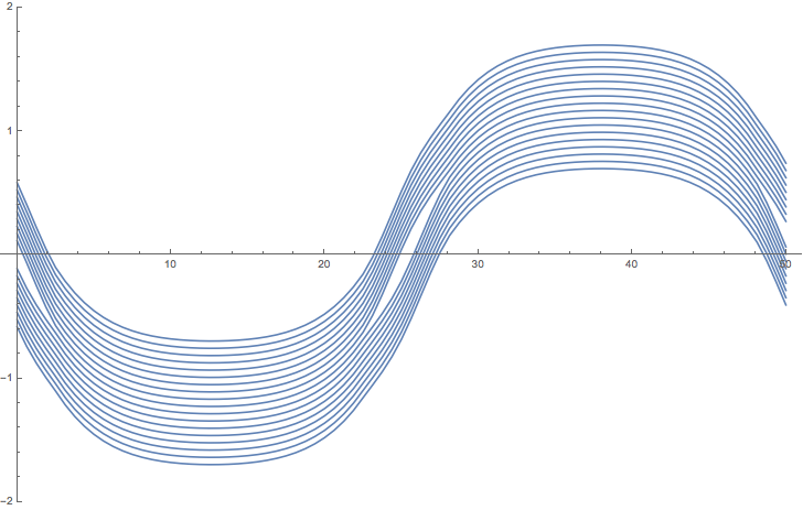
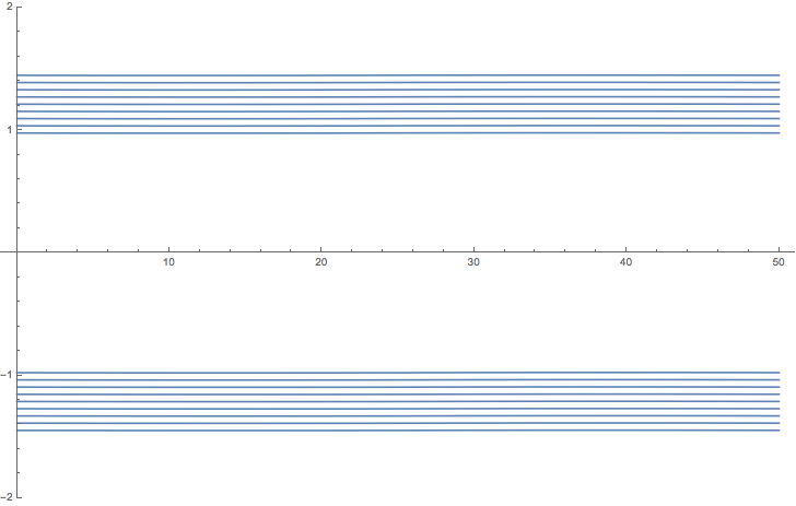
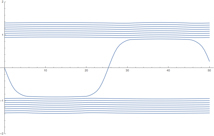
for any J=1,…,N−1J=1,\ldots,N-1, describe completely reciprocal distances between agents at each time tt, and use this fact to prove Theorem 1.2. Note that if (1.8) does not hold, the conclusion of Theorem 1.2 may be false. See Remark 3.5 and the numerical experiments in Section 3.4.

The final step in our analysis is the study of the limit N→∞N\to\infty. First, we define the continuous counterparts of 𝒦TN,𝒦TN,S{\cal K}_{T}^{N},{\cal K}_{T}^{N,S} as follows:

𝒦T\displaystyle{\cal K}_{T} :⁣=\displaystyle:= {(m,w):m∈C(ℝ,𝒫2r(ℝd)),m(t) is T-periodic, \displaystyle\left\{(m,w)\ :\ m\in C({\mathbb{R}},{\cal P}_{2}^{r}({\mathbb{R}}^{d})),\hskip 10.00002ptm(t)\text{ is $T$-periodic, }\right. (1.9)
w is a Borel d-vector measure on ℝ×ℝd, absolutely continuous w.r.t. d​t⊗m⁡(t,d​x),\displaystyle w\text{ is a Borel $d$-vector measure on ${\mathbb{R}}\times{\mathbb{R}}^{d}$, absolutely continuous w.r.t. $dt\otimes m(t,dx)$, }
−∂tm+div(w)=0in the sense of distributions,\displaystyle-\partial_{t}m+{\rm div}(w)=0\ \text{in the sense of distributions, }
∫t1t2∫ℝd12|d​wd​t⊗m⁡(t,d​x)|2m(t,dx)<∞for all −∞<t1<t2<∞},\displaystyle\left.\int_{t_{1}}^{t_{2}}\int_{{\mathbb{R}}^{d}}\frac{1}{2}\left|\frac{dw}{dt\otimes m(t,dx)}\right|^{2}m(t,dx)<\infty\ \text{for all $-\infty<t_{1}<t_{2}<\infty$}\right\},
𝒦TS\displaystyle{\cal K}_{T}^{S} :⁣=\displaystyle:= {(m,w)∈𝒦T:m(−t)=γ#m(t),m(T4+t)=m(T4−t),∀t∈ℝ}.\displaystyle\left\{(m,w)\in{\cal K}_{T}:\ m(-t)=\gamma_{\#}m(t),\ m\left(\frac{T}{4}+t\right)=m\left(\frac{T}{4}-t\right),\forall t\in{\mathbb{R}}\right\}. (1.10)

Then, we have a Γ\Gamma-convergence results for the (constrained) functional JTNJ_{T}^{N} to JTJ_{T}, again in dimension 1.

Theorem 1.3.

Assume (1.3), (1.4), (1.5). Then,

(JTN)|𝒦TN⟶Γ(JT)|𝒦Tas N→+∞,(J_{T}^{N})|_{{\cal K}_{T}^{N}}\stackrel{{\scriptstyle\Gamma}}{{\longrightarrow}}(J_{T})|_{{\cal K}_{T}}\hskip 20.00003pt\text{as $N\to+\infty$,}

with respect to convergence in C⁡([0,T],𝒫2​(ℝ))C([0,T],\mathcal{P}_{2}({\mathbb{R}})) of the empirical measure m𝐱N​(⋅)m_{{\bf x}}^{N}(\cdot) to m⁡(⋅)​d​xm(\cdot)dx and narrow convergence of the empirical measure ∫−T/2T/2δt⊗w𝐱N(t)dt\int_{-T/2}^{T/2}\delta_{t}\otimes w^{N}_{\bf x}(t)dt to w​d​t⊗d​xw\ dt\otimes dx. The same result holds with the additional symmetry constraints, i.e. (JTN)|𝒦TN,S⟶Γ(JT)|𝒦TS(J_{T}^{N})|_{{\cal K}_{T}^{N,S}}\stackrel{{\scriptstyle\Gamma}}{{\longrightarrow}}(J_{T})|_{{\cal K}_{T}^{S}}.

See Theorem 4.1 for a more precise statement of this result. Also in this step, the key difficulty is handling the presence of the distance constraint, in particular in the Γ−lim sup\Gamma-\limsup inequality, that is: given (m,w)∈𝒦T(m,w)\in{\cal K}_{T}, to construct a sequence of competitors 𝐱N{{\bf x}}^{N} whose empirical measures converge to mm. Note that |xit−xjt|≥cN−1/d|x^{i}_{t}-x^{j}_{t}|\geq cN^{-1/d} has to be satisfied. We are not able yet to perform this construction in dimension strictly larger than one.

As a byproduct of the Γ\Gamma-convergence result, minimizers of JTNJ_{T}^{N} converge to minimizers of JTJ_{T}, and their properties pass to the limit: so, under the assumption of strong aggregation (1.8), evenly spaced agents give in the limit a density which is indeed of the form χE⁡(t)\chi_{E(t)}, |E⁡(t)|=1|E(t)|=1. In particular, as it will be stated in Corollary 5.1, we obtain the existence of (mT,wT)∈𝒦TS(m_{T},w_{T})\in{\cal K}_{T}^{S} minimizing JTJ_{T} in 𝒦TS{\cal K}_{T}^{S} such that

mT​(t)=χ(aT​(t),aT​(t)+1)wT​(t)=−a˙T​(t)​χ(aT​(t),aT​(t)+1)m_{T}(t)=\chi_{(a_{T}(t),a_{T}(t)+1)}\hskip 20.00003ptw_{T}(t)=-\dot{a}_{T}(t)\chi_{(a_{T}(t),a_{T}(t)+1)}

where aT:ℝ→[−R0−1,R0]a_{T}:{\mathbb{R}}\to[-R_{0}-1,R_{0}] with R0R_{0} as in (1.5), is a TT-periodic C2C^{2} function minimizing

∫−T/2T/2|x˙t|22dt+∫−T/2T/2∫xtxt+1W(s)dsdt\int_{-T/2}^{T/2}\frac{|\dot{x}_{t}|^{2}}{2}dt+\int_{-T/2}^{T/2}\int_{x_{t}}^{x_{t}+1}W(s)dsdt

among TT periodic curves xtx_{t} such that xt+T4=xT4−tx_{t+\frac{T}{4}}=x_{\frac{T}{4}-t}, and xt=−x−t−1x_{t}=-x_{-t}-1. This shows that the infinite dimensional constrained minimization problem of JTJ_{T} is equivalent to a one dimensional minimization problem for a single representative agent, who observes the averaged potential x↦∫xx+1W⁡(s)​𝑑sx\mapsto\int_{x}^{x+1}W(s)ds.

Acknowledgements

The authors are partially supported by the Fondazione CaRiPaRo Project “Nonlinear Partial Differential Equations: Asymptotic Problems and Mean-Field Games”, and are members of GNAMPA-INdAM. The authors wish to thank D. Gomes for having provided them with a very efficient Mathematica code, which has been used in the numerical analysis of Section 3.4.

2 Preliminary results

2.1 Wasserstein spaces

We briefly recall some notions for calculus in Wasserstein spaces that will be useful in the following. For a general reference on these results we refer to [2, 23]. First, let 𝒫⁡(ℝd)\mathcal{P}({\mathbb{R}}^{d}) be the space of Borel probability measures on ℝd{\mathbb{R}}^{d}, endowed with the topology of narrow convergence, that is:

Definition 2.1.

Let μk,μ∈𝒫⁡(ℝd)\mu_{k},\mu\in\mathcal{P}({\mathbb{R}}^{d}). We say that μk→μ\mu_{k}\to\mu narrowly if

limk∫ℝdg⁡(x)​μk​(𝑑x)=∫ℝdg⁡(x)​μ​(𝑑x)∀g∈Cb​(ℝd),\lim_{k}\int_{{\mathbb{R}}^{d}}g(x)\mu_{k}(dx)=\int_{{\mathbb{R}}^{d}}g(x)\mu(dx)\hskip 20.00003pt\forall g\in C_{b}({\mathbb{R}}^{d}),

where Cb​(ℝd)C_{b}({\mathbb{R}}^{d}) is the space of continuous and bounded functions on ℝd{\mathbb{R}}^{d}.

Note that this convergence is equivalent to convergence in the sense of distributions (see [2, Remark 5.1.6]). We recall also the notion of weak-* convergence in L∞L^{\infty}, that is: for μk,μ∈L∞​(ℝd)\mu_{k},\mu\in L^{\infty}({\mathbb{R}}^{d}), μk\mu_{k} is said to converge to μ\mu weak-* in L∞L^{\infty} if

limk∫ℝdg⁡(x)​μk​(𝑑x)=∫ℝdg⁡(x)​μ​(𝑑x)∀g∈L1​(ℝd).\lim_{k}\int_{{\mathbb{R}}^{d}}g(x)\mu_{k}(dx)=\int_{{\mathbb{R}}^{d}}g(x)\mu(dx)\hskip 20.00003pt\forall g\in L^{1}({\mathbb{R}}^{d}).
Definition 2.2.

Let p≥1p\geq 1. The Wasserstein space of Borel probability measures with bounded pp-moment is defined by

𝒫p​(ℝd)={μ∈𝒫⁡(ℝd)|∫ℝd|x|p​𝑑μ​(x)<+∞}.\mathcal{P}_{p}({\mathbb{R}}^{d})=\left\{\mu\in\mathcal{P}({\mathbb{R}}^{d})\ \Big|\int_{{\mathbb{R}}^{d}}|x|^{p}d\mu(x)<+\infty\right\}.

The Wasserstein space can be endowed with the pp-Wasserstein distance

dp​(μ,ν)p=inf{∫ℝd∫ℝd|x−y|p​𝑑π​(x,y)|π∈π⁡(μ,ν)}d_{p}(\mu,\nu)^{p}=\inf\left\{\int_{{\mathbb{R}}^{d}}\int_{{\mathbb{R}}^{d}}|x-y|^{p}d\pi(x,y)\ |\ \pi\in\pi(\mu,\nu)\right\} (2.1)

where π⁡(μ,ν)\pi(\mu,\nu) is the set of Borel probability measures on ℝd×ℝd{\mathbb{R}}^{d}\times{\mathbb{R}}^{d} such that π⁡(A×ℝd)=μ⁡(A)\pi(A\times{\mathbb{R}}^{d})=\mu(A) and π⁡(ℝd×A)=ν⁡(A)\pi({\mathbb{R}}^{d}\times A)=\nu(A) for any Borel set A⊆ℝdA\subseteq{\mathbb{R}}^{d}.

We introduce a subspace of regular measures as follows

𝒫pr={m∈𝒫p​(ℝd):∃ 0≤m~≤1​ a.e. on ℝd s.t. m=m~​d​x}.{\cal P}_{p}^{r}=\{m\in{\cal P}_{p}({\mathbb{R}}^{d})\ :\ \exists\ 0\leq\tilde{m}\leq 1\ \text{ a.e. on ${\mathbb{R}}^{d}$ s.t. $m=\tilde{m}dx$}\}.

Note that 𝒫p​(ℝd)⊂𝒫q​(ℝd)\mathcal{P}_{p}({\mathbb{R}}^{d})\subset\mathcal{P}_{q}({\mathbb{R}}^{d}) for p<qp<q, and by Jensen inequality, dp​(μ,ν)≤dq​(μ,ν)d_{p}(\mu,\nu)\leq d_{q}(\mu,\nu) for p<qp<q. We then recall the following result about narrow convergence and convergence in Wasserstein spaces.

Lemma 2.3.

𝒫p​(ℝd)\mathcal{P}_{p}({\mathbb{R}}^{d}) endowed with the p-Wasserstein distance is a separable complete metric space. A set ℳ⊆𝒫p​(ℝd)\mathcal{M}\subseteq\mathcal{P}_{p}({\mathbb{R}}^{d}) is relatively compact if and only if it has uniformly integrable pp-moments, that is

limR→+∞supμ∈ℳ∫ℝd∖B⁡(0,R)|x|p​𝑑μ​(x)=0.\lim_{R\to+\infty}\sup_{\mu\in\mathcal{M}}\int_{{\mathbb{R}}^{d}\setminus B(0,R)}|x|^{p}d\mu(x)=0.

Let now μk,μ∈𝒫p​(ℝd)\mu_{k},\mu\in\mathcal{P}_{p}({\mathbb{R}}^{d}) for some p≥1p\geq 1. Then the statements below are equivalent:

  1. (i)

    dp​(μk,μ)→0d_{p}(\mu_{k},\mu)\to 0

  2. (ii)

    μk→μ\mu_{k}\to\mu narrowly and μk\mu_{k} have uniformly integrable pp-moments.

Finally, for any ν∈𝒫p​(ℝd)\nu\in{\cal P}_{p}({\mathbb{R}}^{d}), the map μ→dp​(μ,ν)\mu\to d_{p}(\mu,\nu) is lower semicontinuous with respect to narrow convergence.

Proof.

We refer to [2, Prop. 7.1.5]. Note that if ℳ\mathcal{M} has uniformly integrable pp-moments then it is tight, i.e. for all ε>0\varepsilon>0 there exists Kε⊆ℝdK_{\varepsilon}\subseteq{\mathbb{R}}^{d} compact for which supμ∈ℳ∫ℝd∖Kεd​μ​(x)≤ε\sup_{\mu\in\mathcal{M}}\int_{{\mathbb{R}}^{d}\setminus K_{\varepsilon}}d\mu(x)\leq\varepsilon.

The lower semicontinuity of the Wasserstein distance is proved in [2, Proposition 7.1.3]. ∎

Remark 2.4.

Note that, if for some q>pq>p,

supμ∈ℳ∫ℝd|x|q​𝑑μ​(x)<+∞\sup_{\mu\in\mathcal{M}}\int_{{\mathbb{R}}^{d}}|x|^{q}d\mu(x)<+\infty

then ℳ\mathcal{M} has uniformly integrable pp-moments.

The following semicontinuity and continuity property with respect to narrow convergence and convergence in 𝒫2​(ℝd){\cal P}_{2}({\mathbb{R}}^{d}) respectively will be useful.

Lemma 2.5.

Let μk,μ\mu_{k},\mu be Borel probability measures on ℝd{\mathbb{R}}^{d} such that μk→μ\mu_{k}\to\mu narrowly. Then

lim infk∫ℝdW⁡(x)​μk​(𝑑x)≥∫ℝdW⁡(x)​μ​(𝑑x)\liminf_{k}\int_{{\mathbb{R}}^{d}}W(x)\mu_{k}(dx)\geq\int_{{\mathbb{R}}^{d}}W(x)\mu(dx)

for all lower semicontinuous functions WW.

If moreover WW is as in (1.5) and μk,μ∈𝒫2​(ℝd)\mu_{k},\mu\in\mathcal{P}_{2}({\mathbb{R}}^{d}) then

limkd2​(μk,μ)=0 if and only if limk∫ℝdW⁡(x)​μk​(𝑑x)=∫ℝdW⁡(x)​μ​(𝑑x).\lim_{k}d_{2}(\mu_{k},\mu)=0\hskip 10.00002pt\text{ if and only if }\hskip 10.00002pt\lim_{k}\int_{{\mathbb{R}}^{d}}W(x)\mu_{k}(dx)=\int_{{\mathbb{R}}^{d}}W(x)\mu(dx).
Proof.

For the proof we refer to [2, Lemma 5.1.7] and [9, Lemma 5.7]. ∎

Finally, we recall some results that will be useful in the following about the functional

(μ,w)→∫ℝd12​|d​wd​μ|2​μ​(𝑑x)(\mu,w)\to\int_{{\mathbb{R}}^{d}}\frac{1}{2}\left|\frac{dw}{d\mu}\right|^{2}\mu(dx)

defined on couples (μ,w)(\mu,w) such that μ∈𝒫1​(ℝd)\mu\in{\cal P}_{1}({\mathbb{R}}^{d}) and ww is Borel dd-vector measure on ℝd{\mathbb{R}}^{d}, absolutely continuous w.r.t. μ⁡(d​x)\mu(dx). First of all observe that by Hölder inequality the total variation of |w||w| satisfies

|w|​(ℝd)≤(∫ℝd|d​wd​μ|2​μ​(𝑑x))1/2|w|({\mathbb{R}}^{d})\leq\left(\int_{{\mathbb{R}}^{d}}\left|\frac{dw}{d\mu}\right|^{2}\mu(dx)\right)^{1/2} (2.2)

and moreover the functional is (joint) lower semicontinuous with respect to narrow convergence of measures.

Lemma 2.6.

Let μk,μ∈𝒫⁡(ℝd)\mu_{k},\mu\in\mathcal{P}({\mathbb{R}}^{d}), with μk→μ\mu_{k}\to\mu narrowly. Let wk,w∈𝒫⁡(ℝd,ℝd)w_{k},w\in\mathcal{P}({\mathbb{R}}^{d},{\mathbb{R}}^{d}) be Borel vector measures such that wk→ww_{k}\to w narrowly and wk,ww_{k},w are absolutely continuous with respect to d​t⊗μk​(t,d​x)dt\otimes\mu_{k}(t,dx) and d​t⊗μ⁡(t,d​x)dt\otimes\mu(t,dx), respectively. Then

lim infk∫ℝd|d​wkd​μk|2​d​μk≥∫ℝd|d​wd​μ|2​𝑑μ.\liminf_{k}\int_{{\mathbb{R}}^{d}}\left|\frac{dw_{k}}{d\mu_{k}}\right|^{2}d\mu_{k}\geq\int_{{\mathbb{R}}^{d}}\left|\frac{dw}{d\mu}\right|^{2}d\mu.
Proof.

The result is proved in [2, Lemma 9.4.3]. ∎

The evolutive version of the previous functional is given by

(μ,w)→∫−T/2T/2∫ℝd12|d​wd​t⊗μ⁡(t,d​x)|2μ(t,dx)dt(\mu,w)\to\int_{-T/2}^{T/2}\int_{{\mathbb{R}}^{d}}\frac{1}{2}\left|\frac{dw}{dt\otimes\mu(t,dx)}\right|^{2}\mu(t,dx)dt

defined on couples (μ,w)(\mu,w) such that μ∈C⁡(ℝ,𝒫1​(ℝd))\mu\in C({\mathbb{R}},{\cal P}_{1}({\mathbb{R}}^{d})), ww is a Borel dd-vector measure on ℝ×ℝd{\mathbb{R}}\times{\mathbb{R}}^{d}, absolutely continuous w.r.t. d​t⊗μ⁡(t,d​x)dt\otimes\mu(t,dx). We recall the following uniform continuity property.

Proposition 2.7.

Let (μ,w)(\mu,w) as before and assume that −∂tm+div(w)=0-\partial_{t}m+{\rm div}(w)=0 in the sense of distributions. Then

d22​(μ⁡(t),μ⁡(s))≤|t−s|∫t1t2∫ℝd12​|d​wd​t⊗μ⁡(τ,d​x)|2​μ​(τ,𝑑x)​𝑑τ,∀t,s∈(t1,t2).d_{2}^{2}(\mu(t),\mu(s))\leq|t-s|\int_{t_{1}}^{t_{2}}\int_{{\mathbb{R}}^{d}}\frac{1}{2}\left|\frac{dw}{dt\otimes\mu(\tau,dx)}\right|^{2}\mu(\tau,dx)d\tau,\hskip 20.00003pt\forall t,s\in(t_{1},t_{2}). (2.3)
Proof.

This result is proved in [2, Theorem 8.3.1]. ∎

2.2 Systems with NN agents

Let 𝐱=(x1,…,xN)∈(ℝd)N{\bf x}=(x^{1},\ldots,x^{N})\in({\mathbb{R}}^{d})^{N}, which represents the states of NN agents. We associate to the vector 𝐱{\bf x} the empirical measure

m𝐱N=1N​∑i=1Nδxi.m^{N}_{\bf x}=\frac{1}{N}\sum_{i=1}^{N}\delta_{x^{i}}. (2.4)

We have the following convergence result.

Proposition 2.8.

Let 𝐱∈(ℝd)N{\bf x}\in({\mathbb{R}}^{d})^{N}. Suppose that m𝐱Nm^{N}_{\bf x} converges narrowly to some μ\mu as N→∞N\to\infty and that for some c>0c>0 not depending on NN there holds

|xi−xj|≥cN1/dfor all i≠j.|x^{i}-x^{j}|\geq\frac{c}{N^{1/d}}\hskip 20.00003pt\text{for all $i\neq j$}. (2.5)

Then μ\mu has a density m∈L∞​(ℝd)m\in L^{\infty}({\mathbb{R}}^{d}), and ‖m‖∞≤2d​c−d​ωd−1\|m\|_{\infty}\leq 2^{d}c^{-d}\omega_{d}^{-1}.

Proof.

Note that by narrow convergence ∫ℝdμ⁡(𝑑x)=1\int_{{\mathbb{R}}^{d}}\mu(dx)=1. We prove that μ\mu has a density. Let

δ:=cN1/d\delta:=\frac{c}{N^{1/d}} (2.6)

and ϕ∈Cb​(ℝd)\phi\in C_{b}({\mathbb{R}}^{d}), globally Lipschitz continuous and with ϕ≥0\phi\geq 0. Observe that for every NN, using the bound (2.5) and (2.6),

∫ℝdϕ⁡(y)​m𝐱N​(𝑑y)\displaystyle\int_{{\mathbb{R}}^{d}}\phi(y)m^{N}_{\bf x}(dy) =\displaystyle= ∑iϕ⁡(xi)N=∑i2dωd​cd​∫B⁡(xi,δ/2)[ϕ⁡(xi)−ϕ⁡(y)+ϕ⁡(y)]​𝑑y\displaystyle\sum_{i}\frac{\phi(x^{i})}{N}=\sum_{i}\frac{2^{d}}{\omega_{d}c^{d}}\int_{B(x^{i},\delta/2)}[\phi(x^{i})-\phi(y)+\phi(y)]dy
≤\displaystyle\leq 2dcd​ωd​∑i∫B⁡(xi,δ/2)ϕ⁡(y)​𝑑y+2dcd​ωd​‖∇ϕ‖∞​δ2​ωd​δd2d​N\displaystyle\frac{2^{d}}{c^{d}\omega_{d}}\sum_{i}\int_{B(x^{i},\delta/2)}\phi(y)dy+\frac{2^{d}}{c^{d}\omega_{d}}\|\nabla\phi\|_{\infty}\frac{\delta}{2}\omega_{d}\frac{\delta^{d}}{2^{d}}N
≤\displaystyle\leq 2dcd​ωd​∫ℝdϕ⁡(y)​𝑑y+c​‖∇ϕ‖∞2​N1/d.\displaystyle\frac{2^{d}}{c^{d}\omega_{d}}\int_{{\mathbb{R}}^{d}}\phi(y)dy+\frac{c\|\nabla\phi\|_{\infty}}{2N^{1/d}}.

By narrow convergence we conclude that ∫ℝdϕ⁡(y)​𝑑μ​(y)≤2dcd​ωd​∫ℝdϕ⁡(y)​𝑑y\int_{{\mathbb{R}}^{d}}\phi(y)d\mu(y)\leq\frac{2^{d}}{c^{d}\omega_{d}}\int_{{\mathbb{R}}^{d}}\phi(y)dy for any ϕ∈Cb​(ℝd)\phi\in C_{b}({\mathbb{R}}^{d}), with ϕ≥0\phi\geq 0 and globally Lipschitz. So, for every measurable set AA of finite measure, and every nonnegative smooth mollifier ρ\rho we get that ∫ℝdχA⋆ρ⁡(y)​𝑑μ​(y)≤2dcd​ωd​∫ℝdχA⋆ρ⁡(y)​𝑑y\int_{{\mathbb{R}}^{d}}\chi_{A}\star\rho(y)d\mu(y)\leq\frac{2^{d}}{c^{d}\omega_{d}}\int_{{\mathbb{R}}^{d}}\chi_{A}\star\rho(y)dy, which implies μ⁡(A)≤2dcd​ωd​|A|\mu(A)\leq\frac{2^{d}}{c^{d}\omega_{d}}|A|. This in particular gives that μ\mu has a density mm and that ‖m‖∞≤2dωd​cd\|m\|_{\infty}\leq\frac{2^{d}}{\omega_{d}c^{d}}. ∎

Remark 2.9.

In dimension d=1d=1, we may assume without loss of generality that x1≤x2≤⋯≤xNx^{1}\leq x^{2}\leq\dots\leq x^{N}. Observe that given 𝐱∈ℝN{\bf x}\in{\mathbb{R}}^{N} as in Proposition 2.8 which satisfy in addition |xi−xi+1|=cN|x^{i}-x^{i+1}|=\frac{c}{N} for all i=1,…,N−1i=1,\dots,N-1, then there exists a∈ℝa\in{\mathbb{R}} such that μ=c−1​χ(a,a+c)\mu=c^{-1}\chi_{(a,a+c)}.

Indeed, using that xi+1−xi=cNx^{i+1}-x^{i}=\frac{c}{N} we get that supp​m𝐱N=[x1,x1+c⁡(N−1)N]⊆[x1,x1+c]\text{supp}\ m_{{\bf x}}^{N}=\left[x^{1},x^{1}+\frac{c(N-1)}{N}\right]\subseteq[x^{1},x^{1}+c] for all NN. Therefore since by assumption m𝐱Nm^{N}_{\bf x} converges narrowly to some μ\mu, we get that, eventually passing to a subsequence, x1→ax^{1}\to a as N→+∞N\to+\infty and supp​μ⊆[a,a+c]\text{supp}\mu\subseteq[a,a+c]. Finally, since μ⁡(d​x)=m⁡(x)​d​x\mu(dx)=m(x)dx and 0≤m⁡(x)≤c−10\leq m(x)\leq c^{-1}, then necessarily μ=c−1​χ(a,a+c)\mu=c^{-1}\chi_{(a,a+c)}.

If 𝐱t∈Wper1,2((−T/2,T/2);(ℝd)N){\bf x}_{t}\in W^{1,2}_{\rm per}((-T/2,T/2);({\mathbb{R}}^{d})^{N}), we associate to it the curve of probability measures (representing the dynamic state of NN agents)

m𝐱N​(t)=1N​∑i=1Nδxtim^{N}_{{\bf x}}(t)=\frac{1}{N}\sum_{i=1}^{N}\delta_{x^{i}_{t}} (2.7)

and to 𝐱˙t\dot{\bf x}_{t} the momentum measures

w𝐱N(t):=1N∑i=1Nx˙tiδxti,w~𝐱N:=∫−T/2T/2δt⊗w𝐱N(t)dt∈ℳ([−T/2,T/2]×ℝ).w^{N}_{\bf x}(t):=\frac{1}{N}\sum_{i=1}^{N}\dot{x}_{t}^{i}\delta_{x^{i}_{t}},\hskip 20.00003pt\widetilde{w}^{N}_{\bf x}:=\int_{-T/2}^{T/2}\delta_{t}\otimes w^{N}_{\bf x}(t)dt\in\mathcal{M}([-T/2,T/2]\times{\mathbb{R}}). (2.8)

Note that w~𝐱N​(t)\tilde{w}^{N}_{\bf x}(t) is absolutely continuous with respect to d​t⊗m𝐱N​(t)dt\otimes m_{{\bf x}}^{N}(t), with density d​w𝐱N​(t)d​m𝐱N​(t)=∑i=1Nx˙ti​χx=xti\frac{dw^{N}_{\bf x}(t)}{dm_{{\bf x}}^{N}(t)}=\sum_{i=1}^{N}\dot{x}_{t}^{i}\chi_{x=x^{i}_{t}}. Moreover,

∫ℝ|d​w𝐱N​(t)d​m𝐱N​(t)|2​m𝐱N​(t)​(𝑑x)=1N​∑i=1N|x˙ti|2for a.e. t∈(−T/2,T/2),\int_{\mathbb{R}}\left|\frac{dw^{N}_{\bf x}(t)}{dm_{{\bf x}}^{N}(t)}\right|^{2}m_{{\bf x}}^{N}(t)(dx)=\frac{1}{N}\sum_{i=1}^{N}|\dot{x}^{i}_{t}|^{2}\hskip 20.00003pt\text{for a.e. $t\in(-T/2,T/2)$}, (2.9)

see e.g. [15, Lemma 6.2].

Remark 2.10.

Note that in particular, by (2.3) and (2.9), we get that if 1N∑i=1N∫−T/2T/2|x˙it|2dt≤C\frac{1}{N}\sum_{i=1}^{N}\int_{-T/2}^{T/2}|\dot{x}^{i}_{t}|^{2}dt\leq C, then d22​(m𝐱N​(t),m𝐱N​(s))≤C⁡(t−s)d_{2}^{2}(m^{N}_{\bf x}(t),m^{N}_{\bf x}(s))\leq C(t-s) for all −T/2≤s<t≤T/2-T/2\leq s<t\leq T/2.

2.3 The interaction energy

We define the energy interaction functional for m∈L1​(ℝd)m\in L^{1}({\mathbb{R}}^{d})

ℐ⁡(m)=∫ℝd∫ℝdm⁡(x)​m​(y)​K​(|x−y|)​𝑑x​𝑑y=∫ℝdm⁡(x)​Vm​(x)​𝑑x\mathcal{I}(m)=\int_{{\mathbb{R}}^{d}}\int_{{\mathbb{R}}^{d}}m(x)m(y)K(|x-y|)dxdy=\int_{{\mathbb{R}}^{d}}m(x)V_{m}(x)dx (2.10)

where VmV_{m} is the interaction potential

Vm​(x)=m∗K⁡(x)=∫ℝdm⁡(y)​K​(|x−y|)​𝑑y.V_{m}(x)=m*K(x)=\int_{{\mathbb{R}}^{d}}m(y)K(|x-y|)dy. (2.11)

It is well known that if m∈L1​(ℝd)∩L∞​(ℝd)m\in L^{1}({\mathbb{R}}^{d})\cap L^{\infty}({\mathbb{R}}^{d}) then Vm∈C⁡(ℝd)V_{m}\in C({\mathbb{R}}^{d}) and lim|x|→+∞Vm​(x)=0\lim_{|x|\to+\infty}V_{m}(x)=0 (see [9, Lemma 5.2]).

With a slight abuse of notations, ℐ{\cal I} can be evaluated at m𝐱N=1N​∑i=1Nδxim^{N}_{\bf x}=\frac{1}{N}\sum_{i=1}^{N}\delta_{x^{i}} if xi≠xjx^{i}\neq x^{j} for i≠ji\neq j, in the sense that

ℐ⁡(m𝐱N)=∬ℝ2​d∖ΔK⁡(|x−y|)​m𝐱N​(𝑑x)​m𝐱N​(𝑑y)=1N2​∑i≠jK⁡(|xi−xj|),{\cal I}(m^{N}_{\bf x})=\iint_{{\mathbb{R}}^{2d}\setminus\Delta}K(|x-y|)m^{N}_{\bf x}(dx)m^{N}_{\bf x}(dy)=\frac{1}{N^{2}}\sum_{i\neq j}K(|x^{i}-x^{j}|), (2.12)

where Δ={(x,y)∈ℝd×ℝd:x=y}\Delta=\{(x,y)\in{\mathbb{R}}^{d}\times{\mathbb{R}}^{d}:x=y\}.

We will use the following continuity property of the interaction functional.

Proposition 2.11.

Suppose that 𝐱∈(ℝd)N{\bf x}\in({\mathbb{R}}^{d})^{N} satisfies (2.5) for some cc not depending on NN.

Then,

ℐ⁡(m𝐱N)≤CK{\cal I}(m^{N}_{\bf x})\leq C_{K}

for some positive CKC_{K} that depends on c,d,Kc,d,K (and not on 𝐱,N{\bf x},N).

Assume moreover that m𝐱Nm^{N}_{\bf x} converges narrowly to some μ\mu as N→∞N\to\infty. Then

limNℐ⁡(m𝐱N)=ℐ⁡(m)\lim_{N}{\cal I}(m^{N}_{\bf x})={\cal I}(m)

where m∈L∞​(ℝd)m\in L^{\infty}({\mathbb{R}}^{d}) is the density of μ\mu, given by Proposition 2.8.

Proof.

Let δ\delta as in (2.6) be the bound from below on the distance between xi,xjx^{i},x^{j}. We first deduce a preliminary estimate on ∑j≠i:xj∈Br​(xi)K(|xi−xj|)\sum_{j\neq i:x^{j}\in B_{r}(x^{i})}K(|x^{i}-x^{j}|), for any fixed i=1,…,Ni=1,\ldots,N and r≥δr\geq\delta. To this aim, let x^j:=xj−δ8​xj−xi|xj−xi|\hat{x}^{j}:=x^{j}-\frac{\delta}{8}\frac{x^{j}-x^{i}}{|x^{j}-x^{i}|}. Note that

Bδ8​(x^j)⊂Br​(xi)∀j​ such that ​xj∈Br​(xi),\displaystyle B_{\frac{\delta}{8}}(\hat{x}^{j})\subset B_{r}(x^{i})\hskip 20.00003pt\forall j\text{ such that }x^{j}\in B_{r}(x^{i}),
for all y∈Bδ8​(x^j)y\in B_{\frac{\delta}{8}}(\hat{x}^{j}),   |y−xi|≤|xj−xi||y-x^{i}|\leq|x^{j}-x^{i}|, (2.13)
Bδ8​(x^j)∩Bδ8​(x^k)=∅∀j≠k.\displaystyle B_{\frac{\delta}{8}}(\hat{x}^{j})\cap B_{\frac{\delta}{8}}(\hat{x}^{k})=\emptyset\hskip 20.00003pt\forall j\neq k.

Indeed, since |xj−xi|≥δ|x^{j}-x^{i}|\geq\delta, by the definition of x^j\hat{x}^{j} we get

|x^j−xi|≤|xj−xi−δ8​xj−xi|xj−xi||=||xj−xi|−δ8|=|xj−xi|−δ8≤r,|\hat{x}^{j}-x^{i}|\leq\Big|x^{j}-x^{i}-\frac{\delta}{8}\frac{x^{j}-x^{i}}{|x^{j}-x^{i}|}\Big|=\Big||x^{j}-x^{i}|-\frac{\delta}{8}\Big|=|x^{j}-x^{i}|-\frac{\delta}{8}\leq r,

that yields the first claim. Then, by the triangle inequality and the previous line,

|y−xi|≤|y−x^j|+|x^j−xi|≤δ8+|xj−xi|−δ8=|xj−xi|,|y-x^{i}|\leq|y-\hat{x}^{j}|+|\hat{x}^{j}-x^{i}|\leq\frac{\delta}{8}+|x^{j}-x^{i}|-\frac{\delta}{8}=|x^{j}-x^{i}|,

Finally, since xj∈Bδ8​(x^j)x^{j}\in B_{\frac{\delta}{8}}(\hat{x}^{j}) for all jj,

δ≤|xj−xk|≤|xj−x^j|+|x^j−x^k|+|x^k−xk|≤|x^j−x^k|+δ4,\delta\leq|x^{j}-x^{k}|\leq|x^{j}-\hat{x}^{j}|+|\hat{x}^{j}-\hat{x}^{k}|+|\hat{x}^{k}-x^{k}|\leq|\hat{x}^{j}-\hat{x}^{k}|+\frac{\delta}{4},

hence |x^j−x^k|≥34​δ|\hat{x}^{j}-\hat{x}^{k}|\geq\frac{3}{4}\delta, and Bδ8​(x^j),Bδ8​(x^k)B_{\frac{\delta}{8}}(\hat{x}^{j}),B_{\frac{\delta}{8}}(\hat{x}^{k}) must be disjoint.

Therefore, using the three properties (2.13), and the assumption that K⁡(⋅)K(\cdot) is non-increasing, we get

∑j≠i:xj∈Br​(xi)K(|xi−xj|)=∑j≠i:xj∈Br​(xi)1|Bδ8​(x^j)|∫Bδ8​(x^j)K(|xi−xj|)dy≤∑j≠i:xj∈Br​(xi)1|Bδ8​(0)|∫Bδ8​(x^j)K(|y−xi|)dy=1|Bδ8​(0)|∫⋃jBδ8​(x^j)K(|y−xi|)dy≤1|Bδ8​(0)|​∫Br​(xi)K⁡(|y−xi|)​dy=8d​Ncd​ωd​∫Br​(0)K⁡(|y|)​dy.\sum_{j\neq i:x^{j}\in B_{r}(x^{i})}K(|x^{i}-x^{j}|)=\sum_{j\neq i:x^{j}\in B_{r}(x^{i})}\frac{1}{|B_{\frac{\delta}{8}}(\hat{x}^{j})|}\int_{B_{\frac{\delta}{8}}(\hat{x}^{j})}K(|x^{i}-x^{j}|)dy\\ \leq\sum_{j\neq i:x^{j}\in B_{r}(x^{i})}\frac{1}{|B_{\frac{\delta}{8}}(0)|}\int_{B_{\frac{\delta}{8}}(\hat{x}^{j})}K(|y-x^{i}|)dy=\frac{1}{|B_{\frac{\delta}{8}}(0)|}\int_{\bigcup_{j}B_{\frac{\delta}{8}}(\hat{x}^{j})}K(|y-x^{i}|)dy\\ \leq\frac{1}{|B_{\frac{\delta}{8}}(0)|}\int_{B_{r}(x^{i})}K(|y-x^{i}|)dy=\frac{8^{d}N}{c^{d}\omega_{d}}\int_{B_{r}(0)}K(|y|)dy. (2.14)

A first consequence of this inequality is that

∑j≠iK(|xi−xj|)=∑j≠i:xj∈B1​(xi)K(|xi−xj|)+∑j:xj∈ℝd∖B1​(xi)K(|xi−xj|)≤N⁡(8dcd​ωd​∫B1​(0)K⁡(|y|)​dy+K⁡(1)),\sum_{j\neq i}K(|x^{i}-x^{j}|)=\sum_{j\neq i:x^{j}\in B_{1}(x^{i})}K(|x^{i}-x^{j}|)+\sum_{j:x^{j}\in{\mathbb{R}}^{d}\setminus B_{1}(x^{i})}K(|x^{i}-x^{j}|)\\ \leq N\left(\frac{8^{d}}{c^{d}\omega_{d}}\int_{B_{1}(0)}K(|y|)dy+K(1)\right),

that provides the first stated bound on ℐ⁡(m𝐱N){\cal I}(m^{N}_{\bf x})

ℐ⁡(m𝐱N)=1N​∑i[1N​∑j≠iK⁡(|xi−xj|)]≤(8dcd​ωd​∫B1​(0)K⁡(|y|)​𝑑y+K⁡(1)).{\cal I}(m^{N}_{\bf x})=\frac{1}{N}\sum_{i}\left[\frac{1}{N}\sum_{j\neq i}K(|x^{i}-x^{j}|)\right]\leq\left(\frac{8^{d}}{c^{d}\omega_{d}}\int_{B_{1}(0)}K(|y|)dy+K(1)\right).

We conclude showing the continuity of the interaction energy. For any r>0r>0, define the truncated interaction kernel

Kr​(t):={K⁡(t)if t≥r,K⁡(r)if 0≤t≤r.K_{r}(t):=\begin{cases}K(t)&\text{if $t\geq r$,}\\ K(r)&\text{if $0\leq t\leq r$}.\end{cases}

Since Kr(|⋅x−⋅y|)∈C(ℝ2​d)∩L∞(ℝ2​d)K_{r}(|\cdot_{x}-\cdot_{y}|)\in C({\mathbb{R}}^{2d})\cap L^{\infty}({\mathbb{R}}^{2d}), it is standard (see for example [23, Proposition 7.2]) that

∬ℝ2​dKr​(|x−y|)​m𝐱N​(𝑑x)​m𝐱N​(𝑑y)→∬ℝ2​dKr​(|x−y|)​m​(x)​m​(y)​𝑑x​𝑑yas N→∞.\iint_{{\mathbb{R}}^{2d}}K_{r}(|x-y|)m^{N}_{\bf x}(dx)m^{N}_{\bf x}(dy)\to\iint_{{\mathbb{R}}^{2d}}K_{r}(|x-y|)m(x)m(y)dxdy\hskip 20.00003pt\text{as $N\to\infty$}. (2.15)

Moreover,

ℐ⁡(m𝐱N)=1N2​∑i≠j(K−Kr)​(|xi−xj|)+1N2​∑i≠jKr​(|xi−xj|)=1N∑i[∑j≠i:xj∈Br​(xi)(K−Kr)(|xi−xj|)]+∬ℝ2​dKr(|x−y|)mN𝐱(dx)mN𝐱(dy){\cal I}(m^{N}_{\bf x})=\frac{1}{N^{2}}\sum_{i\neq j}\big(K-K_{r}\big)(|x^{i}-x^{j}|)+\frac{1}{N^{2}}\sum_{i\neq j}K_{r}(|x^{i}-x^{j}|)\\ =\frac{1}{N}\sum_{i}\left[\sum_{j\neq i:x^{j}\in B_{r}(x^{i})}\big(K-K_{r}\big)(|x^{i}-x^{j}|)\right]+\iint_{{\mathbb{R}}^{2d}}K_{r}(|x-y|)m^{N}_{\bf x}(dx)m^{N}_{\bf x}(dy)

Therefore, using (2.14),

|ℐ⁡(m𝐱N)−∬ℝ2​dKr​(|x−y|)​m𝐱N​(𝑑x)​m𝐱N​(𝑑y)|≤C1​∫Br​(0)K⁡(|y|)​𝑑y\Big|{\cal I}(m^{N}_{\bf x})-\iint_{{\mathbb{R}}^{2d}}K_{r}(|x-y|)m^{N}_{\bf x}(dx)m^{N}_{\bf x}(dy)\Big|\leq C_{1}\int_{B_{r}(0)}K(|y|)dy (2.16)

for some C1>0C_{1}>0 not depending on N,rN,r. Note also that since ‖m‖1=1\|m\|_{1}=1,

|ℐ⁡(m)−∬ℝ2​dKr​(|x−y|)​m​(x)​m​(y)​dx​dy|=∬|x−y|≤r(K−Kr)​(|x−y|)​m​(x)​m​(y)​𝑑x​𝑑y≤∫ℝd∫Br​(0)K⁡(|z|)​m​(x+z)​𝑑z​m​(x)​𝑑x≤|m|∫Br​(0)∞⁡K⁡(|z|)​dz.\Big|{\cal I}(m)-\iint_{{\mathbb{R}}^{2d}}K_{r}(|x-y|)m(x)m(y)dxdy\Big|=\\ \iint_{|x-y|\leq r}\big(K-K_{r}\big)(|x-y|)m(x)m(y)dxdy\leq\int_{{\mathbb{R}}^{d}}\int_{B_{r}(0)}K(|z|)m(x+z)dz\,m(x)dx\\ \leq\|m\|_{\infty}\int_{B_{r}(0)}K(|z|)dz. (2.17)

Hence, putting together (2.15), (2.16) and (2.17) we obtain

lim supN→∞|ℐ⁡(m𝐱N)−ℐ⁡(m)|≤(C1+‖m‖∞)​∫Br​(0)K⁡(|y|)​𝑑y,\limsup_{N\to\infty}\Big|{\cal I}(m^{N}_{\bf x})-{\cal I}(m)\Big|\leq(C_{1}+\|m\|_{\infty})\int_{B_{r}(0)}K(|y|)dy,

and since K(|⋅|)K(|\cdot|) is locally in L1L^{1}, we obtain the convergence assertion by letting r→0r\to 0. ∎

2.4 Periodic solutions of the continuous problem

We recall in this section some results obtained in [9] for the mean-field minimization problem over 𝒦T{\cal K}_{T} and 𝒦TS{\cal K}_{T}^{S} (defined in (1.9) and (1.10))

JT(m,w)=∫−T/2T/2∫ℝd12|d​wd​t⊗m⁡(t,d​x)|2m(t,dx)dt+∫−T/2T/2𝒲(m)dt,J_{T}(m,w)=\int_{-T/2}^{T/2}\int_{{\mathbb{R}}^{d}}\frac{1}{2}\left|\frac{dw}{dt\otimes m(t,dx)}\right|^{2}m(t,dx)dt+\int_{-T/2}^{T/2}{\cal W}(m)dt, (2.18)

which is the continuous counterpart of (1.1). The potential part of JTJ_{T} is given by

m↦𝒲⁡(m):=∫ℝdW⁡(x)​m​(𝑑x)−ℐ⁡(m),m∈𝒫2r​(ℝd).m\mapsto\mathcal{W}(m):=\int_{{\mathbb{R}}^{d}}W(x)m(dx)-\mathcal{I}(m),\hskip 20.00003ptm\in{\cal P}_{2}^{r}({\mathbb{R}}^{d}). (2.19)

In the following, we will identify, with a slight abuse of notation, mm and ww with their densities. Note that w∈L2​([−L,L]×ℝd)w\in L^{2}([-L,L]\times{\mathbb{R}}^{d}) for all L>0L>0, due to the fact that

∫t1t2∫ℝd|w|2​𝑑x​𝑑t≤∫t1t2∫ℝd|w⁡(t,x)m⁡(t,x)|2​m​(t,x)​𝑑x​𝑑t.\int_{t_{1}}^{t_{2}}\int_{{\mathbb{R}}^{d}}|w|^{2}dxdt\leq\int_{t_{1}}^{t_{2}}\int_{{\mathbb{R}}^{d}}\left|\frac{w(t,x)}{m(t,x)}\right|^{2}m(t,x)\,dxdt.

Moreover, we recall that elements of 𝒦{\cal K} enjoy the uniform continuity property (2.3).

We recall that minimizers of (2.19) are stationary minimizers (equilibria) of the energy JTJ_{T} over 𝒦T{\cal K}_{T}, but we are interested in particular in constructing non-trivial evolutive critical points. These will be found as minimizers of JTJ_{T} over 𝒦TS{\cal K}_{T}^{S}, which are time periodic and oscillate between stationary solutions. Moreover, sending the period to infinity, it is possible to obtain equilibria which are defined for all times and connect the stationary points. Existence of such families of minimizers have been proved in [9, Theorem 1.1, Theorem 1.2, Theorem 1.3]. We collect here the main results. Note first that symmetry constraints in 𝒦TS,𝒦S{\cal K}^{S}_{T},{\cal K}^{S} are natural, in a sense which will be elaborated in Remark 2.13. Moreover, note also that to guarantee that minima of 𝒲{\cal W} are made up of two disjoint subsets ℳ±\mathcal{M}^{\pm} of 𝒫2r​(ℝd){\cal P}_{2}^{r}({\mathbb{R}}^{d}), we will ask WW to have two sufficiently large plateaus (see the following assumption (2.20)). Such an assumption is not really needed to prove other results for the NN-agents system.

Theorem 2.12.

Assume (1.3), (1.4), (1.5), (1.6), (1.8), and in addition that

{∃a+,a−∈ℝd,r0>0​ such that ​B​(a+,r0)∩B⁡(a−,r0)=∅,|B⁡(a±,r0)|≥1a​n​dW⁡(x)=0⇔x∈B⁡(a+,r0)∪B⁡(a−,r0).\begin{cases}\exists a^{+},a^{-}\in{\mathbb{R}}^{d},r_{0}>0\text{ such that }B(a^{+},r_{0})\cap B(a^{-},r_{0})=\emptyset,\quad|B(a^{\pm},r_{0})|\geq 1\\ \qquad{and}\quad W(x)=0\Leftrightarrow x\in B(a^{+},r_{0})\cup B(a^{-},r_{0}).\end{cases} (2.20)
  1. (i)

    There holds min𝒫2r​(ℝd)⁡𝒲=−ℐ⁡(χBr)\min_{{\cal P}_{2}^{r}({\mathbb{R}}^{d})}{\cal W}=-\mathcal{I}(\chi_{B_{r}}) for r=(ωd)−1/dr=(\omega_{d})^{-1/d}, and all the minimizers of (2.19) are given by ℳ+∪ℳ−\mathcal{M}^{+}\cup\mathcal{M}^{-}, where ℳ−=γ#​ℳ+\mathcal{M}^{-}=\gamma_{\#}\mathcal{M}^{+} and

    ℳ+={χE, where E=B(x′,(ωd)−1/d)⊆B(a+,r0) for some x′∈ℝd}.\mathcal{M}^{+}=\{\chi_{E},\text{ where }E=B(x^{\prime},(\omega_{d})^{-1/d})\subseteq B(a^{+},r_{0})\text{ for some $x^{\prime}\in{\mathbb{R}}^{d}$}\}.

    If |B⁡(a±,r0)|=1|B(a^{\pm},r_{0})|=1, then ℳ±={χB⁡(a±,r)}\mathcal{M}^{\pm}=\{\chi_{B(a^{\pm},r)}\}. ℳ+\mathcal{M}^{+} and ℳ−\mathcal{M}^{-} are compact subsets of 𝒫2​(ℝd)\mathcal{P}_{2}({\mathbb{R}}^{d}), and d2​(ℳ+,ℳ−)>0d_{2}(\mathcal{M^{+}},\mathcal{M^{-}})>0. We define q0:=d2​(ℳ+,ℳ−)/2q_{0}:=d_{2}(\mathcal{M^{+}},\mathcal{M^{-}})/2.

  2. (ii)

    Let q∈(0,q0)q\in(0,q_{0}), where q0q_{0} is defined in the previous item. Then there exists T¯=T¯​(q)>4\bar{T}=\bar{T}(q)>4 such that, for any T≥T¯T\geq\bar{T}, there exists a TT-periodic minimizer (mT,wT)∈𝒦TS(m^{T},w^{T})\in{\cal K}_{T}^{S} of the functional JTJ_{T} in 𝒦TS{\cal K}_{T}^{S}, which satisfies

    {d2​(mT​(t),ℳ+)<q∀t∈(s,T2−s)d2​(mT​(t),ℳ−)<q∀t∈(−T2+s,−s),\begin{cases}d_{2}(m^{T}(t),\mathcal{M}^{+})<q&\forall t\in\left(s,\frac{T}{2}-s\right)\\ d_{2}(m^{T}(t),\mathcal{M}^{-})<q&\forall t\in\left(-\frac{T}{2}+s,-s\right),\end{cases}

    for some 0<s<C=C⁡(q)0<s<C=C(q) (not depending on TT). Moreover T¯​(q)→+∞\bar{T}(q)\to+\infty as q→0q\to 0 and

    limT→+∞d22​(mT​(T4),ℳ+)=0=limT→+∞d22​(mT​(−T4),ℳ−).\lim_{T\to+\infty}d_{2}^{2}\left(m^{T}\left(\frac{T}{4}\right),\mathcal{M}^{+}\right)=0=\lim_{T\to+\infty}d_{2}^{2}\left(m^{T}\left(-\frac{T}{4}\right),\mathcal{M}^{-}\right).

We end up with the following useful observation.

Remark 2.13.

By the convexity of the function (m,w)↦|w|2m(m,w)\mapsto\frac{|w|^{2}}{m} and the regularity of the potential functional 𝒲\mathcal{W} it is possible to show that if (m¯,w¯)∈𝒦TS(\bar{m},\bar{w})\in{\cal K}_{T}^{S} is a minimizer of JTJ_{T} in 𝒦TS{\cal K}_{T}^{S}, then for all (m,w)∈𝒦TS(m,w)\in{\cal K}_{T}^{S}

∫−T/2T/2∫ℝd|w¯​(t,x)m¯​(t,x)|2m¯(t,x)+(W(x)−Vm¯(x))m¯(t,x)dxdt≤∫−T/2T/2∫ℝd|w⁡(t,x)m⁡(t,x)|2m(t,x)+(W(x)−Vm¯(x))m(t,x)dxdt\int_{-T/2}^{T/2}\int_{{\mathbb{R}}^{d}}\left|\frac{\bar{w}(t,x)}{\bar{m}(t,x)}\right|^{2}\bar{m}(t,x)+(W(x)-V_{\bar{m}}(x))\bar{m}(t,x)dxdt\\ \leq\int_{-T/2}^{T/2}\int_{{\mathbb{R}}^{d}}\left|\frac{w(t,x)}{m(t,x)}\right|^{2}m(t,x)+(W(x)-V_{\bar{m}}(x))m(t,x)dxdt (2.21)

where Vm¯V_{\bar{m}} is defined in (2.11). The argument is detailed in [4], see also [11] and is based on the idea of computing the functional JTJ_{T} on OPEN(λ​m¯+(1−λ)​m),λ​w¯+(1−λ)​w)(\lambda\bar{m}+(1-\lambda)m),\lambda\bar{w}+(1-\lambda)w), use convexity of the kinetic part and regularity of the potential part and then send λ→0\lambda\to 0. Such a minimality of (m¯,w¯)(\bar{m},\bar{w}) can be regarded as a mean field Nash equilibrium property.

Moreover, it is possible to show, using the symmetry assumption (1.6), that actually the minimization property (2.21) holds for all competitors (m,w)∈𝒦T(m,w)\in{\cal K}_{T}. For the details we refer to [9, Remark 3.4]. Therefore, following [6], the fact that (m¯,w¯)(\bar{m},\bar{w}) satisfies (2.21) for all (m,w)∈𝒦T(m,w)\in{\cal K}_{T} could be used as a starting point to derive optimality conditions, where an additional “pressure” terms and an ergodic constant will appear due to density constraints and TT-periodicity, whereas no further multipliers related to m⁡(T/4+t)=m⁡(T/4−t)m(T/4+t)=m(T/4-t), m⁡(−t)=γ#​m​(t)m(-t)=\gamma_{\#}m(t) appear in view of the symmetry assumption (1.6).

3 Periodic solutions of the NN-agents system in dimension 11

From now on, we will restrict our study to dimension d=1d=1. We will analyze some qualitative properties of the optimal trajectories of the NN-agents system. That is, we will consider periodic minimizers, with and without symmetries, of JTNJ_{T}^{N}.

We first recall the form of JTNJ_{T}^{N} (which is the discrete counterpart of JTJ_{T}):

JTN(𝐱)=1N∑i=1N∫−T/2T/2|x˙ti|22dt+1N∑i=1N∫−T/2T/2W(xti)dt−1N2∑i≠j∫−T/2T/2K(|xti−xtj|)dt,J_{T}^{N}({\bf x})=\frac{1}{N}\sum_{i=1}^{N}\int_{-T/2}^{T/2}\frac{|\dot{x}^{i}_{t}|^{2}}{2}dt+\frac{1}{N}\sum_{i=1}^{N}\int_{-T/2}^{T/2}W(x^{i}_{t})dt-\frac{1}{N^{2}}\sum_{i\neq j}\int_{-T/2}^{T/2}K\big(|x^{i}_{t}-x^{j}_{t}|\big)dt, (3.1)

where 𝐱∈W1,2​(ℝ,ℝN){\bf x}\in W^{1,2}({\mathbb{R}};{\mathbb{R}}^{N}) and is TT-periodic. Note that JTN​(𝐱)<+∞J_{T}^{N}({\bf x})<+\infty only if xti≠xtjx^{i}_{t}\neq x^{j}_{t} for all i≠ji\neq j and a.e. tt. Recalling (2.9), the functional JTN​(𝐱)J_{T}^{N}({\bf x}) can be equivalently written as (see also (2.12)),

JTN(𝐱)=JT(mN𝐱,wN𝐱)=∫−T/2T/2∫ℝ12|d​w𝐱N​(t)d​m𝐱N​(t)|2m𝐱N(t)(dx)dt+∫−T/2T/2∫ℝW(x)mN𝐱(t)(dx)dt−∫−T/2T/2∫ℝ2∖ΔK(|x−y|)mN𝐱(t)(dx)mN𝐱(t)(dy)dt.J_{T}^{N}({\bf x})=J_{T}(m^{N}_{\bf x},w^{N}_{\bf x})=\int_{-T/2}^{T/2}\int_{{\mathbb{R}}}\frac{1}{2}\left|\frac{dw^{N}_{\bf x}(t)}{dm_{{\bf x}}^{N}(t)}\right|^{2}m_{{\bf x}}^{N}(t)(dx)dt+\int_{-T/2}^{T/2}\int_{{\mathbb{R}}}W(x)m^{N}_{\bf x}(t)(dx)dt\\ -\int_{-T/2}^{T/2}\int_{{\mathbb{R}}^{2}\setminus\Delta}K\big(|x-y|\big)m^{N}_{\bf x}(t)(dx)m^{N}_{\bf x}(t)(dy)dt.

This functional will be considered over 𝒦TN{\cal K}^{N}_{T} and 𝒦TN,S{\cal K}^{N,S}_{T} (defined in (1.7)). Since we have set our problem on the real line, it is convenient to fix the reflection as follows: γ⁡(x)=−x\gamma(x)=-x for all x∈ℝx\in{\mathbb{R}}.

First of all we have a straightforward result about existence of minimizers in 𝒦TN{\cal K}_{T}^{N} and 𝒦TN,S{\cal K}_{T}^{N,S}.

Proof of Theorem 1.1, (i) and (ii).

The proof is based on the classical direct method, so we briefly sketch its argument. First of all we observe that for every 𝐱∈𝒦TN{\bf x}\in{\cal K}_{T}^{N}, by assumption (1.5) and by Proposition 2.11, there exists a constant CKC_{K} depending on the interaction kernel KK and on the dimension dd, but not on NN and 𝐱{\bf x} such that

JTN(𝐱)≥1N∑i=1N∫−T/2T/2|x˙ti|22dt−CWT+CW−1N∑i=1N∫−T/2T/2|xti|2dt−CKT≥−CWT−CKTJ_{T}^{N}({\bf x})\geq\frac{1}{N}\sum_{i=1}^{N}\int_{-T/2}^{T/2}\frac{|\dot{x}^{i}_{t}|^{2}}{2}dt-C_{W}T+\frac{C_{W}^{-1}}{N}\sum_{i=1}^{N}\int_{-T/2}^{T/2}|x^{i}_{t}|^{2}dt-C_{K}T\geq-C_{W}T-C_{K}T

where CWC_{W} is as in (1.5).

We prove just item (ii), since the proof of item (i) is completely analogous (and easier). Let η=inf𝒦TN,SJTN\eta=\inf_{{\cal K}_{T}^{N,S}}J_{T}^{N}. We fix a minimizing sequence 𝐱n{\bf x}_{n}. Since JTN​(𝐱n)≤η+1J_{T}^{N}({\bf x}_{n})\leq\eta+1, we get by the above inequality that 12​N∑i=1N∫−T/2T/2|(x˙ni)t|2dt≤η+1+CKT+CWT\frac{1}{2N}\sum_{i=1}^{N}\int_{-T/2}^{T/2}|(\dot{x}_{n}^{i})_{t}|^{2}dt\leq\eta+1+C_{K}T+C_{W}T. Again, by the same inequality as above we get 1N∑i=1N∫−T/2T/2|(xni)t|2dt≤CW(η+1+CWT+CKT)\frac{1}{N}\sum_{i=1}^{N}\int_{-T/2}^{T/2}|(x_{n}^{i})_{t}|^{2}dt\leq C_{W}(\eta+1+C_{W}T+C_{K}T). Therefore we end up with ‖𝐱n‖Wper1,2​(ℝ,ℝN)≤C\|{\bf x}_{n}\|_{W^{1,2}_{\text{per}}({\mathbb{R}},{\mathbb{R}}^{N})}\leq C, where CC is independent of nn. Therefore by Sobolev embedding 𝐱n{\bf x}_{n} are equi-Hölder continuous, and 𝐱n→𝐱{\bf x}_{n}\to{\bf x} (up to a subsequence) weakly in Wper1,2​(ℝ,ℝN)W^{1,2}_{\text{per}}({\mathbb{R}},{\mathbb{R}}^{N}) and also uniformly. We conclude by uniform convergence that 𝐱∈𝒦TN,S{\bf x}\in{\cal K}_{T}^{N,S}. Moreover 𝐱{\bf x} is a minimizer by weak lower semicontinuity of 12​N∑i=1N∫−T/2T/2|(x˙ni)t|2dt\frac{1}{2N}\sum_{i=1}^{N}\int_{-T/2}^{T/2}|(\dot{x}_{n}^{i})_{t}|^{2}dt and by continuity of 1N∑i=1N∫−T/2T/2W(xti)dt−1N2∑i≠j∫−T/2T/2K(|xti−xtj|)dt\frac{1}{N}\sum_{i=1}^{N}\int_{-T/2}^{T/2}W(x^{i}_{t})dt-\frac{1}{N^{2}}\sum_{i\neq j}\int_{-T/2}^{T/2}K\big(|x^{i}_{t}-x^{j}_{t}|\big)dt.

∎

3.1 Compact support

We now show that periodic minimal solutions of the NN-agents system have a compact support, which is independent of the number of agents

Proof of Theorem 1.1, (iii).

We prove the result only for an 𝐱∈𝒦TN,S{\bf x}\in{\cal K}_{T}^{N,S} which minimizes JTNJ_{T}^{N} in 𝒦TN,S{\cal K}_{T}^{N,S}, since the other case is completely analogous (and even easier). It is enough to prove that mint∈[0,T]⁡xt1≥−R0−1\min_{t\in[0,T]}x^{1}_{t}\geq-R_{0}-1: this would indeed yield for all i,ti,t,

−R0−1≤mint∈[0,T]⁡xt1≤xt1<xti<xtN=−x−t1≤−mint∈[0,T]⁡xt1≤R0+1.-R_{0}-1\leq\min_{t\in[0,T]}x^{1}_{t}\leq x^{1}_{t}<x^{i}_{t}<x^{N}_{t}=-x^{1}_{-t}\leq-\min_{t\in[0,T]}x^{1}_{t}\leq R_{0}+1.

Suppose by contradiction that xt^1<−R0−1x^{1}_{\hat{t}}<-R_{0}-1 for some t^∈[0,T]\hat{t}\in[0,T]. Let x¯ti\bar{x}_{t}^{i} be defined as follows (see Figure 1):

ttℝ{\mathbb{R}}x¯1\bar{x}^{1}x¯2\bar{x}^{2}x¯3\bar{x}^{3}s0s_{0}−s0-s_{0}
Figure 1: An illustration of the truncation procedure in the proof of Theorem 1.1 (iii): x¯i\bar{x}^{i} are defined in (3.2). Dashed lines are the untruncated xix^{i}.
x¯ti:={R0+iNif xti>R0+iNxtiif −R0−N+1−iN≤xti≤R0+iN−R0−N+1−iNif xti<−R0−N+1−iN.\bar{x}_{t}^{i}:=\begin{cases}R_{0}+\frac{i}{N}&\text{if $x_{t}^{i}>R_{0}+\frac{i}{N}$}\\ x_{t}^{i}&\text{if $-R_{0}-\frac{N+1-i}{N}\leq x_{t}^{i}\leq R_{0}+\frac{i}{N}$}\\ -R_{0}-\frac{N+1-i}{N}&\text{if $x_{t}^{i}<-R_{0}-\frac{N+1-i}{N}$}.\end{cases} (3.2)

We first show that 𝐱¯\bar{\bf x} belongs to 𝒦TS,N{\cal K}_{T}^{S,N}. Since −R0−N+1−iN≤x¯ti≤R0+iN-R_{0}-\frac{N+1-i}{N}\leq\bar{x}_{t}^{i}\leq R_{0}+\frac{i}{N}, there hold

{x¯ti≤xti if ​xti≥−R0−N+1−iNx¯ti≥xti if ​xti≤R0+iN.\begin{cases}\bar{x}_{t}^{i}\leq x_{t}^{i}&\text{ if }x_{t}^{i}\geq-R_{0}-\frac{N+1-i}{N}\\ \bar{x}_{t}^{i}\geq x_{t}^{i}&\text{ if }x_{t}^{i}\leq R_{0}+\frac{i}{N}.\end{cases}

By definition, we get

x¯ti+1={R0+i+1N(≥x¯ti+1N)if xti+1>R0+i+1N,xti+1(≥xti+1N≥x¯ti+1N)if −R0−N−iN≤xti+1≤R0+i+1Nand ​xti≥−R0−N+1−iN,xti+1(≥−R0−N−iN=x¯ti+1N)if −R0−N−iN≤xti+1≤R0+i+1Nand ​xti<−R0−N+1−iN,−R0−N−iN(=x¯ti+1N)if xti+1<−R0−N−iN (so xti<−R0−N+1−iN),\bar{x}_{t}^{i+1}=\begin{cases}R_{0}+\frac{i+1}{N}(\geq\bar{x}_{t}^{i}+\frac{1}{N})&\text{if $x_{t}^{i+1}>R_{0}+\frac{i+1}{N}$},\\ x_{t}^{i+1}(\geq x_{t}^{i}+\frac{1}{N}\geq\bar{x}_{t}^{i}+\frac{1}{N})&\begin{array}[]{l}\text{if }-R_{0}-\frac{N-i}{N}\leq x_{t}^{i+1}\leq R_{0}+\frac{i+1}{N}\\ \quad\text{and }x_{t}^{i}\geq-R_{0}-\frac{N+1-i}{N},\end{array}\\ x_{t}^{i+1}(\geq-R_{0}-\frac{N-i}{N}=\bar{x}_{t}^{i}+\frac{1}{N})&\begin{array}[]{l}\text{if }-R_{0}-\frac{N-i}{N}\leq x_{t}^{i+1}\leq R_{0}+\frac{i+1}{N}\\ \quad\text{and }x_{t}^{i}<-R_{0}-\frac{N+1-i}{N},\end{array}\\ -R_{0}-\frac{N-i}{N}(=\bar{x}_{t}^{i}+\frac{1}{N})&\text{if $x_{t}^{i+1}<-R_{0}-\frac{N-i}{N}$ \ (so $x_{t}^{i}<-R_{0}-\frac{N+1-i}{N}$)},\end{cases}

and so we conclude that x¯ti+1≥x¯ti+1N\bar{x}_{t}^{i+1}\geq\bar{x}_{t}^{i}+\frac{1}{N}.

Moreover, since x¯ti=max⁡{min⁡{xti,R0+iN},−R0−N+1−iN}\bar{x}_{t}^{i}=\max\{\min\{x_{t}^{i},R_{0}+\frac{i}{N}\},-R_{0}-\frac{N+1-i}{N}\},

x¯tN+1−i=max⁡{min⁡{xtN+1−i,R0+N+1−iN},−R0−iN}=−min⁡{max⁡{x−ti,−R0−N+1−iN},R0+iN}=−x¯−ti,\bar{x}_{t}^{N+1-i}=\max\left\{\min\left\{x_{t}^{N+1-i},R_{0}+\frac{N+1-i}{N}\right\},-R_{0}-\frac{i}{N}\right\}=\\ -\min\left\{\max\left\{x_{-t}^{i},-R_{0}-\frac{N+1-i}{N}\right\},R_{0}+\frac{i}{N}\right\}=-\bar{x}_{-t}^{i},

and x¯T4+ti=x¯T4−ti\bar{x}^{i}_{\frac{T}{4}+t}=\bar{x}^{i}_{\frac{T}{4}-t} follows analogously.

We can now evaluate JTN​(𝐱¯)J_{T}^{N}(\bar{\bf x}). Recalling that W′​(s)<0W^{\prime}(s)<0 for all s<−R0s<-R_{0} and W′​(s)>0W^{\prime}(s)>0 for all s>R0s>R_{0} by symmetry assumptions on WW we get that

W⁡(x¯ti)={W⁡(R0+iN)<W⁡(xti)if xti>R0+iNW⁡(xti)if −R0−N+1−iN≤xti≤R0+iNW⁡(−R0−N+1−iN)<W⁡(xti)if xti<−R0−N+1−iN.W(\bar{x}_{t}^{i})=\begin{cases}W(R_{0}+\frac{i}{N})<W(x_{t}^{i})&\text{if $x_{t}^{i}>R_{0}+\frac{i}{N}$}\\ W(x_{t}^{i})&\text{if $-R_{0}-\frac{N+1-i}{N}\leq x_{t}^{i}\leq R_{0}+\frac{i}{N}$}\\ W(-R_{0}-\frac{N+1-i}{N})<W(x_{t}^{i})&\text{if $x_{t}^{i}<-R_{0}-\frac{N+1-i}{N}$}.\end{cases}

Since we are supposing that xt^1<−R0−1x^{1}_{\hat{t}}<-R_{0}-1, by continuity of t↦xt^1t\mapsto x^{1}_{\hat{t}} we have xt1<−R0−1x^{1}_{t}<-R_{0}-1 for all tt in a neighborhood of t^\hat{t}, and therefore

1N∑i=1N∫−T/2T/2W(x¯ti)dt<1N∑i=1N∫−T/2T/2W(xti)dt.\frac{1}{N}\sum_{i=1}^{N}\int_{-T/2}^{T/2}W(\bar{x}^{i}_{t})dt<\frac{1}{N}\sum_{i=1}^{N}\int_{-T/2}^{T/2}W(x^{i}_{t})dt. (3.3)

In addition, by the definition (3.2) of 𝐱¯\bar{\bf x} it is clear that

1N∑i=1N∫−T/2T/2|x¯˙it|2dt≤1N∑i=1N∫−T/2T/2|x˙it|2dt.\frac{1}{N}\sum_{i=1}^{N}\int_{-T/2}^{T/2}|\dot{\bar{x}}^{i}_{t}|^{2}dt\leq\frac{1}{N}\sum_{i=1}^{N}\int_{-T/2}^{T/2}|\dot{x}^{i}_{t}|^{2}dt. (3.4)

Finally, to evaluate the interaction energy, first of all we observe that reciprocal distances between agents do not increase in this truncation procedure: indeed

x¯ti+1−x¯ti={R0+i+1N−R0−iN=1Nif xti>R0+iN (so xti+1>R0+i+1N),R0+i+1N−xti≤xti+1−xtiif −R0−N+1−iN≤xti≤R0+iN,and ​xti+1>R0+i+1N,xti+1−xtiif −R0−N+1−iN≤xti≤R0+iN,and ​xti+1≤R0+i+1N,xti+1+R0+N+1−iN<xti+1−xtiif ​xti<−R0−N+1−iNand ​xti+1≥−R0−N−iN,−R0−N−iN+R0+N+1−iN=1Nif ​xti<−R0−N+1−iNand ​xti+1<−R0−N−iN,\bar{x}_{t}^{i+1}-\bar{x}_{t}^{i}=\begin{cases}R_{0}+\frac{i+1}{N}-R_{0}-\frac{i}{N}=\frac{1}{N}&\text{if $x_{t}^{i}>R_{0}+\frac{i}{N}$ \ (so $x_{t}^{i+1}>R_{0}+\frac{i+1}{N}$)},\\ R_{0}+\frac{i+1}{N}-x_{t}^{i}\leq x_{t}^{i+1}-x_{t}^{i}&\begin{array}[]{l}\text{if $-R_{0}-\frac{N+1-i}{N}\leq x_{t}^{i}\leq R_{0}+\frac{i}{N}$},\\ \quad\text{and }x_{t}^{i+1}>R_{0}+\frac{i+1}{N},\end{array}\\ x_{t}^{i+1}-x_{t}^{i}&\begin{array}[]{l}\text{if $-R_{0}-\frac{N+1-i}{N}\leq x_{t}^{i}\leq R_{0}+\frac{i}{N}$},\\ \quad\text{and }x_{t}^{i+1}\leq R_{0}+\frac{i+1}{N},\end{array}\\ x_{t}^{i+1}+R_{0}+\frac{N+1-i}{N}<x_{t}^{i+1}-x_{t}^{i}&\begin{array}[]{l}\text{if }x_{t}^{i}<-R_{0}-\frac{N+1-i}{N}\\ \quad\text{and }x_{t}^{i+1}\geq-R_{0}-\frac{N-i}{N},\end{array}\\ -R_{0}-\frac{N-i}{N}+R_{0}+\frac{N+1-i}{N}=\frac{1}{N}&\begin{array}[]{l}\text{if }x_{t}^{i}<-R_{0}-\frac{N+1-i}{N}\\ \quad\text{and }x_{t}^{i+1}<-R_{0}-\frac{N-i}{N},\end{array}\end{cases}

so x¯ti+1−x¯ti≤xti+1−xti\bar{x}_{t}^{i+1}-\bar{x}_{t}^{i}\leq x_{t}^{i+1}-x_{t}^{i}, that implies |x¯tj−x¯ti|≤|xtj−xti||\bar{x}_{t}^{j}-\bar{x}_{t}^{i}|\leq|x_{t}^{j}-x_{t}^{i}| for all i,j,ti,j,t. Therefore, monotonicity of K⁡(⋅)K(\cdot) yields K⁡(|x¯ti−x¯tj|)≥K⁡(|xti−xtj|)K(|\bar{x}_{t}^{i}-\bar{x}_{t}^{j}|)\geq K(|x_{t}^{i}-x_{t}^{j}|) for all i,j,ti,j,t, and then

−1N2∑i≠j∫−T/2T/2K(|x¯ti−x¯tj|)dt≤−1N2∑i≠j∫−T/2T/2K(|xti−xtj|)dt.-\frac{1}{N^{2}}\sum_{i\neq j}\int_{-T/2}^{T/2}K\big(|\bar{x}^{i}_{t}-\bar{x}^{j}_{t}|\big)dt\leq-\frac{1}{N^{2}}\sum_{i\neq j}\int_{-T/2}^{T/2}K\big(|x^{i}_{t}-x^{j}_{t}|\big)dt. (3.5)

Hence, adding (3.3), (3.4) and (3.5) provides

JTN​(𝐱¯)<JTN​(𝐱),J_{T}^{N}(\bar{\bf x})<J_{T}^{N}({\bf x}),

which contradicts the minimality of 𝐱{\bf x}. ∎

3.2 Optimality conditions

In this section we derive optimality conditions for the minimizers of the functional JTNJ_{T}^{N}, in the sets 𝒦TN{\cal K}_{T}^{N} and 𝒦TN,S{\cal K}_{T}^{N,S}. These will be crucial in the proof of Theorem 1.2. Due to the distance constraints, the optimality conditions are given in terms of inequalities, and hold as equalities on intervals where the constraints is not saturated. First of all we start observing that, as shown in the continuous case in Remark 2.10, in the optimality conditions no further multipliers due to the symmetry conditions appear.

Remark 3.1.

Let 𝐱\bf x be a minimizer of JTNJ_{T}^{N} on 𝒦TN,S{\cal K}_{T}^{N,S}. First of all we observe that 𝐱\bf x minimizes on 𝒦TN,S{\cal K}_{T}^{N,S} the following linearized functional:

J¯TN(𝐲;𝐱):=1N∑i=1N∫−T/2T/2x˙ity˙itdt+1N∑i=1N∫−T/2T/2W′(xit)yitdt−1N2∑i≠j∫−T/2T/2K′(|xit−xjt|)xti−xtj|xti−xtj|(yit−yjt)dt.\overline{J}_{T}^{N}({\bf y};{\bf x}):=\frac{1}{N}\sum_{i=1}^{N}\int_{-T/2}^{T/2}\dot{x}^{i}_{t}\dot{y}^{i}_{t}dt+\frac{1}{N}\sum_{i=1}^{N}\int_{-T/2}^{T/2}W^{\prime}(x^{i}_{t})y^{i}_{t}dt\\ -\frac{1}{N^{2}}\sum_{i\neq j}\int_{-T/2}^{T/2}K^{\prime}\big(|x^{i}_{t}-x^{j}_{t}|\big)\frac{x^{i}_{t}-x^{j}_{t}}{|x^{i}_{t}-x^{j}_{t}|}(y^{i}_{t}-y^{j}_{t})dt. (3.6)

To prove this, we fix 𝐲∈𝒦TN,S{\bf y}\in{\cal K}_{T}^{N,S} and we denote by 𝐲λ:=(1−λ)​𝐱+λ​𝐲{\bf y}^{\lambda}:=(1-\lambda){\bf x}+\lambda{\bf y} for all λ∈[0,1]\lambda\in[0,1]. Since 𝐲λ∈𝒦TN,S{\bf y}^{\lambda}\in{\cal K}_{T}^{N,S} there holds

0≤\displaystyle 0\leq JTN​(𝐲λ)−JTN​(𝐱)λ=1N∑i=1N∫−T/2T/2x˙ti(y˙ti−x˙ti)dt+λ2​N∑i=1N∫−T/2T/2|y˙ti|2−|x˙ti|2dt\displaystyle\frac{J_{T}^{N}({\bf y}^{\lambda})-J_{T}^{N}({\bf x})}{\lambda}=\frac{1}{N}\sum_{i=1}^{N}\int_{-T/2}^{T/2}\dot{x}^{i}_{t}(\dot{y}^{i}_{t}-\dot{x}^{i}_{t})dt+\frac{\lambda}{2N}\sum_{i=1}^{N}\int_{-T/2}^{T/2}|\dot{y}^{i}_{t}|^{2}-|\dot{x}^{i}_{t}|^{2}dt
+1N∑i=1N∫−T/2T/2W⁡(xti+λ⁡(yti−xti))−W⁡(xti)λdt\displaystyle+\frac{1}{N}\sum_{i=1}^{N}\int_{-T/2}^{T/2}\frac{W(x^{i}_{t}+\lambda(y^{i}_{t}-x^{i}_{t}))-W(x^{i}_{t})}{\lambda}dt
−1N2∑i≠j∫−T/2T/2K⁡(|xti−xtj+λ⁡(yti−ytj−xti+xtj)|)−K⁡(|xti−xtj|)λdt\displaystyle-\frac{1}{N^{2}}\sum_{i\neq j}\int_{-T/2}^{T/2}\frac{K\big(|x^{i}_{t}-x^{j}_{t}+\lambda(y^{i}_{t}-y^{j}_{t}-x^{i}_{t}+x^{j}_{t})|\big)-K\big(|x^{i}_{t}-x^{j}_{t}|\big)}{\lambda}dt

from which we conclude sending λ→0\lambda\to 0.

In addition we get that 𝐱{\bf x} is a minimizer of J¯TN\overline{J}_{T}^{N} in a more general class of non-symmetric competitors:

J¯TN​(𝐳,𝐱)≥J¯TN​(𝐱,𝐱)for all 𝐳∈𝒦TN.\overline{J}_{T}^{N}({\bf z};{\bf x})\geq\overline{J}_{T}^{N}({\bf x};{\bf x})\hskip 20.00003pt\text{for all ${\bf z}\in{\cal K}_{T}^{N}$}. (3.7)

Indeed, let 𝐳∈𝒦TN{\bf z}\in{\cal K}_{T}^{N}, such that zT4+ti=zT4−tiz^{i}_{\frac{T}{4}+t}=z^{i}_{\frac{T}{4}-t}. Define

yti:=zti−z−tN+1−i2,wti:=zti+z−tN+1−i2zti=yti+wti.y^{i}_{t}:=\frac{z^{i}_{t}-z^{N+1-i}_{-t}}{2},\hskip 20.00003ptw^{i}_{t}:=\frac{z^{i}_{t}+z^{N+1-i}_{-t}}{2}\hskip 20.00003ptz^{i}_{t}=y^{i}_{t}+w^{i}_{t}.

It is straightforward to check that yti−yti−1=zti−zti−12+z−tN+2−i−z−tN+1−i2≥1Ny^{i}_{t}-y^{i-1}_{t}=\frac{z^{i}_{t}-z^{i-1}_{t}}{2}+\frac{z^{N+2-i}_{-t}-z^{N+1-i}_{-t}}{2}\geq\frac{1}{N}, and yti=−y−tN+1−iy^{i}_{t}=-y_{-t}^{N+1-i}, so 𝐲∈𝒦TN,S{\bf y}\in{\cal K}_{T}^{N,S}.

Moreover wtN+1−i=w−tiw^{N+1-i}_{t}=w^{i}_{-t}. By this, and recalling xtN+1−i=−x−tix^{N+1-i}_{t}=-x^{i}_{-t} and that W′​(s)=−W′​(−s)W^{\prime}(s)=-W^{\prime}(-s) by (1.6), we obtain J¯TN​(𝐰,𝐱)=0\overline{J}_{T}^{N}({\bf w};{\bf x})=0. So, by linearity, we conclude

J¯TN​(𝐳,𝐱)=J¯TN​(𝐲,𝐱)+J¯TN​(𝐰,𝐱)=J¯TN​(𝐲,𝐱)≥J¯TN​(𝐱,𝐱).\overline{J}_{T}^{N}({\bf z};{\bf x})=\overline{J}_{T}^{N}({\bf y};{\bf x})+\overline{J}_{T}^{N}({\bf w};{\bf x})=\overline{J}_{T}^{N}({\bf y};{\bf x})\geq\overline{J}_{T}^{N}({\bf x};{\bf x}).

To prove that the previous inequality holds without the assumption zT4+ti=zT4−tiz^{i}_{\frac{T}{4}+t}=z^{i}_{\frac{T}{4}-t}, one can argue in a similar way, using the decomposition zti=12​(zti+zT2−ti)+12​(zti−zT2−ti)z^{i}_{t}=\frac{1}{2}(z^{i}_{t}+z^{i}_{\frac{T}{2}-t})+\frac{1}{2}(z^{i}_{t}-z^{i}_{\frac{T}{2}-t}).

For J=1,…,N−1J=1,\ldots,N-1, let us consider the mean of (xtJ+1,…,xtN)(x_{t}^{J+1},\ldots,x_{t}^{N}) and the mean of (xt1,…,xtJ)(x_{t}^{1},\ldots,x_{t}^{J}), i.e.

x¯tJ+1:=1N−J​∑i=J+1Nxti,x¯tJ:=1J​∑i=1Jxti.{\overline{x}}_{t}^{J+1}:=\frac{1}{N-J}\sum_{i=J+1}^{N}x^{i}_{t},\hskip 20.00003pt{\underline{x}}^{J}_{t}:=\frac{1}{J}\sum_{i=1}^{J}x^{i}_{t}. (3.8)
ttℝ{\mathbb{R}}x¯tJ{{\underline{x}}^{J}_{t}\ \Big\{x¯tJ+1{{\overline{x}}^{J+1}_{t}\ \big\{
Figure 2:

See Figure 2. We first show that if 𝐱{\bf x} is a minimizer of JTNJ_{T}^{N} either in 𝒦TN,S{\cal K}_{T}^{N,S} or in 𝒦TN{\cal K}_{T}^{N}, then x¯tJ+1{\overline{x}}_{t}^{J+1} and x¯tJ{\underline{x}}_{t}^{J} solve useful differential inequalities.

Lemma 3.2.

Suppose that 𝐱\bf x minimizes JTNJ_{T}^{N} on 𝒦TN,S{\cal K}_{T}^{N,S} (or on 𝒦TN{\cal K}_{T}^{N}, in which case (𝐱t)′≡0({\bf x}_{t})^{\prime}\equiv 0). Then, for any J=1,…,N−1J=1,\ldots,N-1,

−(x¯tJ+1)′′+1(N−J)​∑i≥J+1W′​(xti)−2N⁡(N−J)​∑i≥J+1j≤JK′​(|xti−xtj|)≥0\displaystyle\displaystyle-({\overline{x}}_{t}^{J+1})^{\prime\prime}+\frac{1}{(N-J)}\sum_{i\geq J+1}W^{\prime}(x^{i}_{t})-\frac{2}{N(N-J)}\sum_{\begin{subarray}{c}i\geq J+1\\ j\leq J\end{subarray}}K^{\prime}\big(|x^{i}_{t}-x^{j}_{t}|\big)\geq 0 (3.9)
(x¯tJ)′′−1J​∑i≤JW′​(xti)−2N​J​∑i≥J+1j≤JK′​(|xti−xtj|)≥0\displaystyle\displaystyle({\underline{x}}_{t}^{J})^{\prime\prime}-\frac{1}{J}\sum_{i\leq J}W^{\prime}(x^{i}_{t})-\frac{2}{NJ}\sum_{\begin{subarray}{c}i\geq J+1\\ j\leq J\end{subarray}}K^{\prime}\big(|x^{i}_{t}-x^{j}_{t}|\big)\geq 0 (3.10)

in the weak sense in ℝ{\mathbb{R}}.

If, in addition, xtJ+1>xtJ+1Nx_{t}^{J+1}>x_{t}^{J}+\frac{1}{N} for some J=1,…,NJ=1,\ldots,N in an open set Ω⊆ℝ\Omega\subseteq{\mathbb{R}}, then

−(x¯tJ+1)′′+1(N−J)​∑i≥J+1W′​(xti)−2N⁡(N−J)​∑i≥J+1j≤JK′​(|xti−xtj|)=0\displaystyle\displaystyle-({\overline{x}}_{t}^{J+1})^{\prime\prime}+\frac{1}{(N-J)}\sum_{i\geq J+1}W^{\prime}(x^{i}_{t})-\frac{2}{N(N-J)}\sum_{\begin{subarray}{c}i\geq J+1\\ j\leq J\end{subarray}}K^{\prime}\big(|x^{i}_{t}-x^{j}_{t}|\big)=0
(x¯tJ)′′−1J​∑i≤JW′​(xti)−2N​J​∑i≥J+1j≤JK′​(|xti−xtj|)=0\displaystyle\displaystyle({\underline{x}}_{t}^{J})^{\prime\prime}-\frac{1}{J}\sum_{i\leq J}W^{\prime}(x^{i}_{t})-\frac{2}{NJ}\sum_{\begin{subarray}{c}i\geq J+1\\ j\leq J\end{subarray}}K^{\prime}\big(|x^{i}_{t}-x^{j}_{t}|\big)=0

in the weak sense in Ω\Omega.

Proof.

If 𝐱\bf x is a minimizer of JTNJ_{T}^{N} on 𝒦TN,S{\cal K}_{T}^{N,S}, by Remark 3.1 𝐱{\bf x} is a minimizer of the linearized functional J¯TN​(𝐲,𝐱)\overline{J}_{T}^{N}({\bf y};{\bf x}) in 𝒦TN{\cal K}_{T}^{N}, so we do not impose any symmetry conditions on the competitors to derive the optimality conditions. Let ψ∈Cper∞​(ℝ)\psi\in C^{\infty}_{\rm per}({\mathbb{R}}), ψ≥0\psi\geq 0 on ℝ{\mathbb{R}}, and

x~ti:={xti+ψ⁡(t)if J+1≤i≤Nxtiif 1≤i≤Jfor all t.\tilde{x}^{i}_{t}:=\begin{cases}x^{i}_{t}+\psi(t)&\text{if $J+1\leq i\leq N$}\\ x^{i}_{t}&\text{if $1\leq i\leq J$}\end{cases}\hskip 20.00003pt\text{for all $t$.}

Note that x~ti\tilde{x}^{i}_{t} consists of trajectories where xtix^{i}_{t} is shifted “upwards” whenever i≥J+1i\geq J+1. Since x~i+1≥x~i+1N\tilde{x}^{i+1}\geq\tilde{x}^{i}+\frac{1}{N}, we have 𝐱~∈𝒦TN\tilde{\bf x}\in{\cal K}_{T}^{N}.

Note that

∑i≠j∫−T/2T/2K′(|xit−xjt|)xti−xtj|xti−xtj|(x~it−x~jt)dt−∑i≠j∫−T/2T/2K′(|xit−xjt|)xti−xtj|xti−xtj|(xit−xjt)dt=−∫−T/2T/2∑i≤Jj≥J+1K′(|xit−xjt|)xti−xtj|xti−xtj|ψ(t)+∫−T/2T/2∑i≥J+1j≤JK′(|xit−xjt|)xti−xtj|xti−xtj|ψ(t)=2∫−T/2T/2∑i≥J+1j≤JK′(|xit−xjt|)ψ(t)dt.\sum_{i\neq j}\int_{-T/2}^{T/2}K^{\prime}\big(|x^{i}_{t}-x^{j}_{t}|\big)\frac{x^{i}_{t}-x^{j}_{t}}{|x^{i}_{t}-x^{j}_{t}|}(\tilde{x}^{i}_{t}-\tilde{x}^{j}_{t})dt-\sum_{i\neq j}\int_{-T/2}^{T/2}K^{\prime}\big(|x^{i}_{t}-x^{j}_{t}|\big)\frac{x^{i}_{t}-x^{j}_{t}}{|x^{i}_{t}-x^{j}_{t}|}(x^{i}_{t}-x^{j}_{t})dt=\\ -\int_{-T/2}^{T/2}\sum_{\begin{subarray}{c}i\leq J\\ j\geq J+1\end{subarray}}K^{\prime}\big(|x^{i}_{t}-x^{j}_{t}|\big)\frac{x^{i}_{t}-x^{j}_{t}}{|x^{i}_{t}-x^{j}_{t}|}\psi(t)+\int_{-T/2}^{T/2}\sum_{\begin{subarray}{c}i\geq J+1\\ j\leq J\end{subarray}}K^{\prime}\big(|x^{i}_{t}-x^{j}_{t}|\big)\frac{x^{i}_{t}-x^{j}_{t}}{|x^{i}_{t}-x^{j}_{t}|}\psi(t)\\ =2\int_{-T/2}^{T/2}\sum_{\begin{subarray}{c}i\geq J+1\\ j\leq J\end{subarray}}K^{\prime}\big(|x^{i}_{t}-x^{j}_{t}|\big)\psi(t)dt.

Therefore, by the minimum property (3.7) of 𝐱{\bf x},

0≤J¯TN​(𝐱~,𝐱)−J¯TN​(𝐱,𝐱)=∫−T/2T/21N∑i≥J+1x˙itψ˙(t)+1N∑i≥J+1W′(xit)ψ(t)dt−2N2∑i≥J+1j≤JK′(|xit−xjt|)ψ(t)dt.0\leq\overline{J}_{T}^{N}(\tilde{\bf x};{\bf x})-\overline{J}_{T}^{N}({\bf x};{\bf x})=\\ \int_{-T/2}^{T/2}\frac{1}{N}\sum_{i\geq J+1}\dot{x}^{i}_{t}\dot{\psi}(t)+\frac{1}{N}\sum_{i\geq J+1}W^{\prime}(x^{i}_{t})\psi(t)dt-\frac{2}{N^{2}}\sum_{\begin{subarray}{c}i\geq J+1\\ j\leq J\end{subarray}}K^{\prime}\big(|x^{i}_{t}-x^{j}_{t}|\big)\psi(t)dt.

Multiplying the previous inequality by N/[N−J]N/[N-J] yields the weak inequality for x¯tJ+1{\overline{x}}^{J+1}_{t}.

To prove the weak inequality for x¯tJ{\underline{x}}^{J}_{t} one can argue similarly, considering competitors of the form

x~ti:={xtiif J+1≤i≤Nxti−ψ⁡(t)if 1≤i≤Jfor all t.\tilde{x}^{i}_{t}:=\begin{cases}x^{i}_{t}&\text{if $J+1\leq i\leq N$}\\ x^{i}_{t}-\psi(t)&\text{if $1\leq i\leq J$}\end{cases}\hskip 20.00003pt\text{for all $t$.}

Variations of J¯TN\overline{J}_{T}^{N} yield the following inequality in the weak sense

(x¯tJ)′′−1J​∑i≤JW′​(xti)−2N​J​∑i≥J+1j≤JK′​(|xti−xtj|)≥0.\displaystyle({\underline{x}}_{t}^{J})^{\prime\prime}-\frac{1}{J}\sum_{i\leq J}W^{\prime}(x^{i}_{t})-\frac{2}{NJ}\sum_{\begin{subarray}{c}i\geq J+1\\ j\leq J\end{subarray}}K^{\prime}\big(|x^{i}_{t}-x^{j}_{t}|\big)\geq 0.

in ℝ{\mathbb{R}}.

Finally, if xtJ+1>xtJ+1Nx_{t}^{J+1}>x_{t}^{J}+\frac{1}{N} for some J=1,…,NJ=1,\ldots,N in an open set Ω⊂(0,T/2)\Omega\subset(0,T/2), then it is possible to perturb trajectories in the opposite direction in space (i.e. “downwards”), being the constraint xtJ+1=xtJ+1Nx_{t}^{J+1}=x_{t}^{J}+\frac{1}{N} inactive. In particular, for small ε>0\varepsilon>0 and ψ∈Cper∞​(ℝ)\psi\in C^{\infty}_{\rm per}({\mathbb{R}}), it is possible to look at first order variations of the form

x~tε,i:={xti−ε​ψ​(t)if J+1≤i≤Nxtiif 1≤i≤Jfor all t∈Ω,\tilde{x}^{\varepsilon,i}_{t}:=\begin{cases}x^{i}_{t}-\varepsilon\psi(t)&\text{if $J+1\leq i\leq N$}\\ x^{i}_{t}&\text{if $1\leq i\leq J$}\end{cases}\hskip 20.00003pt\text{for all $t\in\Omega$,}

that yield the desired equalities. ∎

Lemma 3.3.

Suppose that 𝐱\bf x minimizes JTNJ_{T}^{N} on 𝒦TN{\cal K}_{T}^{N} (or on 𝒦TN,S{\cal K}_{T}^{N,S}), and that xtJ+1>xtJ+1Nx_{t}^{J+1}>x_{t}^{J}+\frac{1}{N} for some J=1,…,NJ=1,\ldots,N in an open set Ω⊆ℝ\Omega\subseteq{\mathbb{R}}. Then, the map t↦x¯tJ+1−x¯tJt\mapsto{\overline{x}}_{t}^{J+1}-{\underline{x}}_{t}^{J} is of class C2​(Ω)C^{2}(\Omega), and

(x¯tJ−x¯tJ+1)′′+1(N−J)​∑i≥J+1W′​(xti)−1J​∑i≤JW′​(xti)−2N​J∑i≥J+1j≤JK′(|xit−xjt|)−2N⁡(N−J)∑i≥J+1j≤JK′(|xit−xjt|)=0\displaystyle({\underline{x}}_{t}^{J}-{\overline{x}}_{t}^{J+1})^{\prime\prime}+\frac{1}{(N-J)}\sum_{i\geq J+1}W^{\prime}(x^{i}_{t})-\frac{1}{J}\sum_{i\leq J}W^{\prime}(x^{i}_{t})\\ -\frac{2}{NJ}\sum_{\begin{subarray}{c}i\geq J+1\\ j\leq J\end{subarray}}K^{\prime}\big(|x^{i}_{t}-x^{j}_{t}|\big)-\frac{2}{N(N-J)}\sum_{\begin{subarray}{c}i\geq J+1\\ j\leq J\end{subarray}}K^{\prime}\big(|x^{i}_{t}-x^{j}_{t}|\big)=0 (3.11)

in Ω\Omega. Moreover,

(x¯tJ+1−x¯tJ)′′≥2​min0<r≤2​R0+2​|K′​(r)|−2​max|x|≤R0+1​|W′​(x)|in Ω.({\overline{x}}_{t}^{J+1}-{\underline{x}}_{t}^{J})^{\prime\prime}\geq 2\min_{0<r\leq 2R_{0}+2}|K^{\prime}(r)|-2\max_{|x|\leq R_{0}+1}|W^{\prime}(x)|\hskip 20.00003pt\text{in $\Omega$}.
Proof.

The equality (3.11) in the weak sense follows directly by Lemma 3.2. Note that curves xtix^{i}_{t} belong to W1,2​(0,T)W^{1,2}(0,T), and therefore they are of class C1/2​(Ω)C^{1/2}(\Omega). Thus, t↦x¯tJ+1−x¯tJt\mapsto{\overline{x}}_{t}^{J+1}-{\underline{x}}_{t}^{J} is of class C2​(Ω)C^{2}(\Omega), with 1/21/2-Hölder second order derivative, and (3.11) holds in the classical pointwise sense.

Recall that in view of Theorem 1.1 (iii), optimal trajectories xtix^{i}_{t} are bounded independently of i,t,Ni,t,N, that is |xti|≤R0+1|x^{i}_{t}|\leq R_{0}+1 for all t∈[0,T]t\in[0,T] and i=1,…​Ni=1,\ldots N. So, in particular, ±W′​(xti)≥−max|x|≤R0+1⁡|W′​(x)|\pm W^{\prime}(x^{i}_{t})\geq-\max_{|x|\leq R_{0}+1}|W^{\prime}(x)| for all i,ti,t. On the other hand, −K′​(|xti−xtj|)≥−max0<r≤2​R0+2⁡K′​(r)=min0<r≤2​R0+2⁡|K′​(r)|-K^{\prime}\big(|x^{i}_{t}-x^{j}_{t}|\big)\geq-\max_{0<r\leq 2R_{0}+2}K^{\prime}(r)=\min_{0<r\leq 2R_{0}+2}|K^{\prime}(r)|, since KK is nonincreasing, Therefore by (3.11) we get that in Ω\Omega there holds

(x¯tJ+1−x¯tJ)′′≥\displaystyle({\overline{x}}_{t}^{J+1}-{\underline{x}}_{t}^{J})^{\prime\prime}\geq −max|x|≤R0+1⁡|W′​(x)|​(1(N−J)​∑i≥J+11+1J​∑i≤J1)\displaystyle\ -\max_{|x|\leq R_{0}+1}|W^{\prime}(x)|\left(\frac{1}{(N-J)}\sum_{i\geq J+1}1+\frac{1}{J}\sum_{i\leq J}1\right)
+min0<r≤2​R0+2⁡|K′​(r)|​(2N​J​∑i≥J+1j≤J1+2N⁡(N−J)​∑i≥J+1j≤J1)\displaystyle+\min_{0<r\leq 2R_{0}+2}|K^{\prime}(r)|\left(\frac{2}{NJ}\sum_{\begin{subarray}{c}i\geq J+1\\ j\leq J\end{subarray}}1+\frac{2}{N(N-J)}\sum_{\begin{subarray}{c}i\geq J+1\\ j\leq J\end{subarray}}1\right)
=−2​max|x|≤R0+1​|W′​(x)|+2​min0<r≤2​R0+2​|K′​(r)|.\displaystyle=-2\max_{|x|\leq R_{0}+1}|W^{\prime}(x)|+2\min_{0<r\leq 2R_{0}+2}|K^{\prime}(r)|.

∎

3.3 Saturation of the distance constraint

Finally, we show that minimizers saturate the distance constraints under the further assumption (1.8).

Proof of Theorem 1.2.

As for Theorem 1.1 (iii), we will prove the result only for 𝐱∈𝒦TN,S{\bf x}\in{\cal K}_{T}^{N,S} minimizing JTNJ_{T}^{N} in 𝒦TN,S{\cal K}_{T}^{N,S}, being the other case is completely analogous (and even easier). Define, as in Appendix A,

dti=di​(𝐱t):=xti−xti−1,for i=2,…,N,d^{i}_{t}=d^{i}({\bf x}_{t}):=x_{t}^{i}-x_{t}^{i-1},\hskip 20.00003pt\text{for $i=2,\ldots,N$},

and

𝐦tJ=𝐦J​(𝐱t):=x¯tJ+1−x¯tJ=1N−J​∑i=J+1Nxti−1J​∑i=1Jxtifor J=1,…,N−1.{\bf m}^{J}_{t}={\bf m}^{J}({\bf x}_{t}):={\overline{x}}_{t}^{J+1}-{\underline{x}}_{t}^{J}=\frac{1}{N-J}\sum_{i=J+1}^{N}x^{i}_{t}-\frac{1}{J}\sum_{i=1}^{J}x^{i}_{t}\hskip 20.00003pt\text{for $J=1,\ldots,N-1$}.

Let t^\hat{t} be a time at which the (periodic) map t↦𝐦t1t\mapsto{\bf m}^{1}_{t} reaches its global maximum on ℝ{\mathbb{R}}. We first claim that dt^2=xt^2−xt^1=1Nd^{2}_{\hat{t}}=x^{2}_{\hat{t}}-x^{1}_{\hat{t}}=\frac{1}{N}. If the claim is not true, then xt2−xt1>1Nx^{2}_{t}-x^{1}_{t}>\frac{1}{N} for all tt in a neighborhood Ω\Omega of t^\hat{t}. In this case, by Lemma 3.3, 𝐦t1{\bf m}^{1}_{t} is of class C2​(Ω)C^{2}(\Omega), and since it reaches a maximum at t=t^t=\hat{t}, (𝐦1)t^′=0({\bf m}^{1})^{\prime}_{\hat{t}}=0. Moreover by (1.8)

(𝐦t1)′′≥2​min0<r≤2​R0+2​|K′​(r)|−2​max|x|≤R0+1​|W′​(x)|>0in Ω,({\bf m}^{1}_{t})^{\prime\prime}\geq 2\min_{0<r\leq 2R_{0}+2}|K^{\prime}(r)|-2\max_{|x|\leq R_{0}+1}|W^{\prime}(x)|>0\hskip 10.00002pt\text{in $\Omega$},

but this contradicts the fact that 𝐦t1{\bf m}^{1}_{t} has a maximum at t=t^t=\hat{t}. Then dt^2=xt^2−xt^1=1Nd^{2}_{\hat{t}}=x^{2}_{\hat{t}}-x^{1}_{\hat{t}}=\frac{1}{N}, and since xt2−xt1≥1Nx^{2}_{t}-x^{1}_{t}\geq\frac{1}{N} for all tt, the map t↦dt2t\mapsto d^{2}_{t} has a global minimum at t=t^t=\hat{t}. In view of Lemma A.1,

𝐦t2=N−1N−2​𝐦t1−N2​(N−2)​dt2,{\bf m}^{2}_{t}=\frac{N-1}{N-2}{\bf m}_{t}^{1}-\frac{N}{2(N-2)}d_{t}^{2},

hence t^\hat{t} is also a global maximum for t↦𝐦t2t\mapsto{\bf m}^{2}_{t}.

It is possible to show in the same way by induction that t^\hat{t} is a global maximum for t↦𝐦tit\mapsto{\bf m}^{i}_{t} for any i=1,…,N−1i=1,\ldots,N-1, and that dt^j=1Nd^{j}_{\hat{t}}=\frac{1}{N} for all j=2,…,Nj=2,\ldots,N. Indeed, suppose that the previous claim is true for i,j≤Ji,j\leq J; we need to show its validity for i,j=J+1i,j=J+1. First, dt^J+1=1Nd^{J+1}_{\hat{t}}=\frac{1}{N}, otherwise xtJ+1−xtJ>1Nx^{J+1}_{t}-x^{J}_{t}>\frac{1}{N} for all tt in a neighborhood Ω\Omega of t^\hat{t}. Hence, by Lemma 3.3, 𝐦tJ{\bf m}^{J}_{t} is of class C2​(Ω)C^{2}(\Omega), and (𝐦J)t^′=0({\bf m}^{J})^{\prime}_{\hat{t}}=0. Moreover,

(𝐦tJ)′′≥2​min0<r≤2​R0+2​|K′​(r)|−2​max|x|≤R0+1​|W′​(x)|>0in Ω,({\bf m}^{J}_{t})^{\prime\prime}\geq 2\min_{0<r\leq 2R_{0}+2}|K^{\prime}(r)|-2\max_{|x|\leq R_{0}+1}|W^{\prime}(x)|>0\hskip 10.00002pt\text{in $\Omega$},

but this contradicts the fact that 𝐦tJ{\bf m}^{J}_{t} has a maximum at t=t^t=\hat{t}, yielding that t↦dtJ+1t\mapsto d^{J+1}_{t} has a global minimum at t=t^t=\hat{t} that is equal to 1N\frac{1}{N}. In view of Lemma A.1,

𝐦tJ+1=N−1N−J−1​𝐦1−∑j=1J(N−jN−J−1−jJ+1)​dj+1,{\bf m}^{J+1}_{t}=\frac{N-1}{N-J-1}{\bf m}^{1}-\sum_{j=1}^{J}\left(\frac{N-j}{N-J-1}-\frac{j}{J+1}\right)d^{j+1},

and since (N−jN−J−1−jJ+1)>0\left(\frac{N-j}{N-J-1}-\frac{j}{J+1}\right)>0, t^\hat{t} is also a global maximum for t↦𝐦tJ+1t\mapsto{\bf m}^{J+1}_{t}.

Having obtained that dt^j=1Nd^{j}_{\hat{t}}=\frac{1}{N} for all j=2,…,Nj=2,\ldots,N, we may conclude by Lemma A.2 (with α=1N\alpha=\frac{1}{N}) that 𝐦t^J=12{\bf m}^{J}_{\hat{t}}=\frac{1}{2} for all J=1,…,N−1J=1,\ldots,N-1. Since 12\frac{1}{2} is the minimal value of 𝐦tJ{\bf m}^{J}_{t}, and 𝐦tJ{\bf m}^{J}_{t} reaches its maximum at t^\hat{t}, the only possibility is 𝐦tJ=12{\bf m}^{J}_{t}=\frac{1}{2} for all t∈[0,T]t\in[0,T]. Applying again Lemma A.2 we get that xtj−xtj−1=dtj=1Nx^{j}_{t}-x^{j-1}_{t}=d^{j}_{t}=\frac{1}{N} for all tt and jj. ∎

Remark 3.4.

We observe that, due to Theorem 1.2, the minimization problem (3.1) in 𝒦TN,S{\cal K}_{T}^{N,S} is actually 11-dimensional.

We compute the energy of a minimizer 𝐱∈𝒦TN,S{\bf x}\in{\cal K}_{T}^{N,S} of JTNJ_{T}^{N} in 𝒦TN,S{\cal K}_{T}^{N,S}. We define the function

W¯N​(x):=1N​∑i=0N−1W⁡(x+iN)\overline{W}_{N}(x):=\frac{1}{N}\sum_{i=0}^{N-1}W\left(x+\frac{i}{N}\right) (3.12)

and the positive constant

KN:=1N2​∑i≠j∈{0,…,N−1}K⁡(|i−jN|).K^{N}:=\frac{1}{N^{2}}\sum_{i\neq j\in\{0,\dots,N-1\}}K\left(\left|\frac{i-j}{N}\right|\right).

Note that KN≤CKK^{N}\leq C_{K} for all NN by Proposition 2.11.

Since by Theorem 1.2 xti=xt1+i−1Nx_{t}^{i}=x_{t}^{1}+\frac{i-1}{N} and x˙ti=x˙tj\dot{x}_{t}^{i}=\dot{x}_{t}^{j} for all i,j,ti,j,t, there holds

JTN(𝐱)=∫−T/2T/2|x˙t1|22dt+∫−T/2T/2W¯N(xt1)dt−KNT.J_{T}^{N}({\bf x})=\int_{-T/2}^{T/2}\frac{|\dot{x}^{1}_{t}|^{2}}{2}dt+\int_{-T/2}^{T/2}\overline{W}_{N}\left(x^{1}_{t}\right)dt-K^{N}T.

Moreover, again using that xti=xt1+i−1Nx_{t}^{i}=x_{t}^{1}+\frac{i-1}{N}, by the symmetry condition we get

xt1+i−1N=xti=−x−tN+1−i=−x−t1−N−iN, and then ​xt1=−x−t1−N−1N​∀t.x_{t}^{1}+\frac{i-1}{N}=x_{t}^{i}=-x_{-t}^{N+1-i}=-x_{-t}^{1}-\frac{N-i}{N},\text{ \hskip 10.00002ptand then \ }x_{t}^{1}=-x_{-t}^{1}-\frac{N-1}{N}\ \forall t.

This in particular forces

x01=−N−12​N=xT/21 and x˙t1=x˙−t1.x^{1}_{0}=-\frac{N-1}{2N}=x^{1}_{T/2}\hskip 10.00002pt\text{ and }\hskip 10.00002pt\dot{x}_{t}^{1}=\dot{x}_{-t}^{1}.

Using these symmetries, and recalling that W⁡(s)=W⁡(−s)W(s)=W(-s) we get

JTN​(𝐱)=2​∫0T/2|x˙t1|22​𝑑t+2​∫0T/2W¯N​(xt1)​𝑑t−KN​T:=J~T1​(x1).J_{T}^{N}({\bf x})=2\int_{0}^{T/2}\frac{|\dot{x}^{1}_{t}|^{2}}{2}dt+2\int_{0}^{T/2}\overline{W}_{N}\left(x^{1}_{t}\right)dt-K^{N}T:=\tilde{J}_{T}^{1}(x^{1}). (3.13)

We observe that if 𝐱{\bf x} is a minimizer of JTNJ_{T}^{N} in 𝒦TN,S{\cal K}_{T}^{N,S}, then xt1x^{1}_{t} is a minimizer of J~T1\tilde{J}^{1}_{T} on the set

𝒦~T1,S:={y∈W1,2([0,T2];ℝ):y0=−N−12​N,yT4+t=yT4−t∀t∈[0,T/4]}.\tilde{\cal K}_{T}^{1,S}:=\left\{y\in W^{1,2}\left(\left[0,\frac{T}{2}\right];{\mathbb{R}}\right)\ :\ y_{0}=-\frac{N-1}{2N},\ y_{\frac{T}{4}+t}=y_{\frac{T}{4}-t}\ \forall\ t\in[0,T/4]\right\}.

Indeed if y∈K~T1,Sy\in\tilde{K}_{T}^{1,S}, we may construct 𝐲∈W1,2​(ℝ,ℝN){\bf y}\in W^{1,2}({\mathbb{R}};{\mathbb{R}}^{N}) as follows: first of all we extend yy on [−T/2,0][-T/2,0] putting y−t=−yt−N−1Ny_{-t}=-y_{t}-\frac{N-1}{N}, extend it to be a TT periodic function, and finally define yti:=yt+i−1Ny_{t}^{i}:=y_{t}+\frac{i-1}{N} for i=0,…,Ni=0,\dots,N. It is easy to check that 𝐲∈𝒦TN,S{\bf y}\in{\cal K}_{T}^{N,S} and that JTN​(𝐲)=J~T1​(y)J_{T}^{N}({\bf{y}})=\tilde{J}^{1}_{T}(y), This permits to conclude, by minimality of 𝐱{\bf x}.

Reasoning as in Remark 3.1, we get that xt1x^{1}_{t} is a minimizer of the following functional

J¯T1​(y,x1):=2​∫0T/2x˙t1​y˙t​𝑑t+2​∫0T/2W¯N′​(xt1)​yt​𝑑t\overline{J}_{T}^{1}(y;x^{1}):=2\int_{0}^{T/2}\dot{x}^{1}_{t}\dot{y}_{t}dt+2\int_{0}^{T/2}\overline{W}_{N}^{\prime}(x^{1}_{t})y_{t}dt

among all y∈W1,2​((0,T/2),ℝ)y\in W^{1,2}((0,T/2);{\mathbb{R}}) such that y0=yT/2=−N−12​Ny_{0}=y_{T/2}=-\frac{N-1}{2N}. Indeed we use the decomposition yt=zt+wt:=12​(yt+yT2−t)+12​(yt−yT2−t)y_{t}=z_{t}+w_{t}:=\frac{1}{2}(y_{t}+y_{\frac{T}{2}-t})+\frac{1}{2}(y_{t}-y_{\frac{T}{2}-t}). It is easy to chech that zt+T/4=zT/4−tz_{t+T/4}=z_{T/4-t} and z0=zT/2=N−12​Nz_{0}=z_{T/2}=\frac{N-1}{2N}, so w∈K~T1,Sw\in\tilde{K}_{T}^{1,S}, whereas wt+T/4=−wT/4−tw_{t+T/4}=-w_{T/4-t} and w0=0=wT/2w_{0}=0=w_{T/2}. It is easy to check that J¯T1​(w)=0\overline{J}_{T}^{1}(w)=0, using the fact that t→xT/4+t1t\to x^{1}_{T/4+t} is even whereas t↦w⁡(T/4+t)t\mapsto w(T/4+t) is odd. So, by linearity we get J¯T1​(y)=J¯T1​(z)\overline{J}_{T}^{1}(y)=\overline{J}_{T}^{1}(z) and we conclude.

Let if ϕ∈Cc∞​(0,T/2)\phi\in C^{\infty}_{c}(0,T/2), then yt=xt1+δ​ϕ​(t)∈W1,2​((0,T/2),ℝ)y_{t}=x^{1}_{t}+\delta\phi(t)\in W^{1,2}((0,T/2);{\mathbb{R}}) is such that y0=yT/2=−N−12​Ny_{0}=y_{T/2}=-\frac{N-1}{2N}. We compute

0≤J¯T1​(y,x1)−J¯T1​(x1,x1)δ=2​∫0T/2x˙t1​ϕ˙​(t)​𝑑t+2​∫0T/2W¯N′​(xt1)​ϕ​(t)​𝑑t0\leq\frac{\overline{J}_{T}^{1}(y;x^{1})-\overline{J}_{T}^{1}(x^{1};x^{1})}{\delta}=2\int_{0}^{T/2}\dot{x}^{1}_{t}\dot{\phi}(t)dt+2\int_{0}^{T/2}\overline{W}_{N}^{\prime}(x^{1}_{t})\phi(t)dt

and then xt1x_{t}^{1} is a TT-periodic solution to

{(xt1)′′=W¯N′​(xt1)=1N​∑i=0N−1W′​(xt1+iN)t∈ℝx01=−N−12​N=xT/21.\begin{cases}(x_{t}^{1})^{\prime\prime}=\overline{W}_{N}^{\prime}(x^{1}_{t})=\frac{1}{N}\sum_{i=0}^{N-1}W^{\prime}\left(x^{1}_{t}+\frac{i}{N}\right)&t\in{\mathbb{R}}\\ x_{0}^{1}=-\frac{N-1}{2N}=x_{T/2}^{1}.\end{cases} (3.14)

Since W∈C1​(ℝ)W\in C^{1}({\mathbb{R}}) by (1.5), t↦xt1t\mapsto x_{t}^{1} is a C2C^{2} function, with supt|(xt1)′′|≤max[−R0−1,R0+1]⁡|W′​(s)|\sup_{t}|(x_{t}^{1})^{\prime\prime}|\leq\max_{[-R_{0}-1,R_{0}+1]}|W^{\prime}(s)|.

Remark 3.5.

We now observe that non stationary minimizers may not saturate the distance constraint in general. Supposing that some given K0,WK_{0},W satisfy the standing assumption, then K=α​K0K=\alpha K_{0} satisfies as well the same assumptions for any α>0\alpha>0. If α\alpha is large enough (and K0′<0K_{0}^{\prime}<0), then Theorem 1.2 states that minimizing trajectories minimize reciprocal distances. On the other hand, if α\alpha is small this property may not hold. Consider indeed a potential WW that, in addition to (1.5), vanishes on [−3,−2]∪[2,3][-3,-2]\cup[2,3] and satisfies W≥1W\geq 1 on [−1,1][-1,1]. Let 𝐱∈𝒦TN{\bf x}\in{\cal K}_{T}^{N} be any minimizer of JTNJ_{T}^{N} in 𝒦TN{\cal K}_{T}^{N} and assume by contradiction that

xti+1=xti+1Nfor all t and ix^{i+1}_{t}=x^{i}_{t}+\frac{1}{N}\hskip 20.00003pt\text{for all $t$ and $i$} (3.15)

holds. We first estimate JTN​(x)J_{T}^{N}(x) from above via a suitable competitor 𝐲∈𝒦TN{\bf y}\in{\cal K}_{T}^{N}. For NN odd,

yti:={−2+iNi<N+12,0i=N+12,−(−2+N+1−iN)i>N+12.y^{i}_{t}:=\begin{cases}-2+\frac{i}{N}&i<\frac{N+1}{2},\\ 0&i=\frac{N+1}{2},\\ -\left(-2+\frac{N+1-i}{N}\right)&i>\frac{N+1}{2}.\end{cases}

Then,

∫−T/2T/2|x˙tN+12|22dt+∫−T/2T/21N∑iW(xti)dt−αK0NT≤JTN(x)≤JTN(y)≤TNW(0).\int_{-T/2}^{T/2}\frac{|\dot{x}^{\frac{N+1}{2}}_{t}|^{2}}{2}dt+\int_{-T/2}^{T/2}\frac{1}{N}\sum_{i}W(x^{i}_{t})dt-\alpha K_{0}^{N}T\leq J_{T}^{N}(x)\leq J_{T}^{N}(y)\leq\frac{T}{N}W(0).

Note that x0N+12=0x^{\frac{N+1}{2}}_{0}=0. Moreover, ∫−T/2T/2|x˙tN+12|22dt\int_{-T/2}^{T/2}\frac{|\dot{x}^{\frac{N+1}{2}}_{t}|^{2}}{2}dt can be bounded by a constant that does not depend on NN and α≤1\alpha\leq 1, so there exists δ>0\delta>0 such that |xtN+12|≤1/2|x^{\frac{N+1}{2}}_{t}|\leq 1/2 for all t∈(−δ,δ)t\in(-\delta,\delta). By (3.15), |xti|≤1|x^{i}_{t}|\leq 1 and W⁡(xti)≥1W(x^{i}_{t})\geq 1 for all ii and t∈(−δ,δ)t\in(-\delta,\delta), and δ\delta does not depend on NN. Thus,

JTN​(x)≥∫−δδ1N​∑iW⁡(xti)​𝑑t−α​K0N​T≥2​δ−α​CK0​T,J_{T}^{N}(x)\geq\int_{-\delta}^{\delta}\frac{1}{N}\sum_{i}W(x^{i}_{t})dt-\alpha K_{0}^{N}T\geq 2\delta-\alpha C_{K_{0}}T,

and for α\alpha small and NN large JTN​(x)≥2​δ−2​α​I​(χ(0,1))​T>TN​W​(0)≥JTN​(y)J_{T}^{N}(x)\geq 2\delta-2\alpha I(\chi_{(0,1)})T>\frac{T}{N}W(0)\geq J_{T}^{N}(y) which is a contradiction.

3.4 Some numerical experiments

We now show a few numerical approximations of minimizers of the functional JTNJ^{N}_{T} (on 𝒦TN,S{\cal K}^{N,S}_{T}). These have been obtained using a gradient descent method, with the following choice of the data:

K0​(r)=1r,W⁡(x)=10​((0.5−x2)a,++(x2−3)a,+),T=50,K_{0}(r)=\frac{1}{\sqrt{r}},\hskip 20.00003ptW(x)=10\Big((0.5-x^{2})^{a,+}+(x^{2}-3)^{a,+}\Big),\hskip 20.00003ptT=50,

where (x)a,+:=(.1​1+(10​x)2+x)/2(x)^{a,+}:=(.1\sqrt{1+(10x)^{2}}+x)/2 is a regularized version of the positive part of xx. Though WW does not satisfy our standing assumptions (it does not have truly flat regions), it is very close to zero on ±[1/2,3CLOSE\pm[\sqrt{1/2},\sqrt{3}]. In our results, shown in Figure 3, three different scenarios show up. When the non-local aggregative kernel is strong enough, that is when K=5​K0K=5K_{0}, periodic trajectories are evenly spaced on the whole time interval. This is in line with the assertion of Theorem 1.2. On the other hand, with a mild interaction kernel (K=K0K=K_{0} in our pictures), agents split into two groups, that occupy the two wells (the example in Remark 3.5 is inspired by this scenario). When the number of agents NN is odd, the middle (N+1)/2(N+1)/2-th agent oscillates between the two groups which are located in the wells, while if NN is even then groups are simmetrically distributed. There is a final intermediate case, e.g. when K=3.1​K0K=3.1K_{0}, where the aggregation force is mild, and agents break down into two groups. In this case, it is not convenient for agents to saturate always the constraint, but to create some gap between two temporary groups while crossing the region of the potential between the two wells.
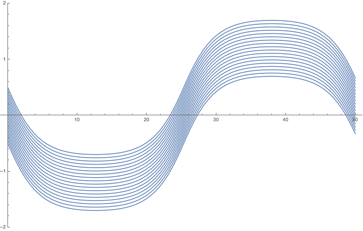
N=18,K=5​K0N=18,\ K=5K_{0} N=18,K=3.1​K0N=18,\ K=3.1K_{0}
Refer to caption Refer to caption
N=18,K=K0N=18,\ K=K_{0} N=17,K=K0N=17,\ K=K_{0}
Refer to caption Refer to caption
Figure 3: Minimizers of JTNJ_{T}^{N} in 𝒦TN,S{\cal K}_{T}^{N,S} for different choices of the interaction kernel KK and number of agents NN. Every line represents the evolution of a single agent. Time tt and position xtix_{t}^{i} are in the horizontal and vertical axis respectively.

4 Γ\Gamma-convergence as N→+∞N\to+\infty and convergence of minimizers in dimension 11

In this section we provide the Γ\Gamma-convergence as N→+∞N\to+\infty of the discrete energies JTNJ_{T}^{N} defined in (3.1) for 𝐱∈𝒦TN{\bf x}\in\mathcal{K}_{T}^{N} (or 𝐱∈𝒦TN,S{\bf x}\in{\cal K}_{T}^{N,S}) to the energy JTJ_{T}, defined in (2.18), for (m,w)∈𝒦T(m,w)\in\mathcal{K}_{T} (resp. (m,w)∈𝒦TS(m,w)\in{\cal K}_{T}^{S}). Moreover, we provide convergence of minimal solutions of the NN-agent system to minimal solutions of the mean-field problem. This result is based on a standard application of the Γ\Gamma-convergence result, and coercivity of the involved functionals.

First of all we extend the energies to include the constraints as follows

JT​(m,w)={JT​(m,w)if ​(m,w)∈𝒦T+∞ otherwiseJTN​(𝐱)={JTN​(𝐱)if ​𝐱∈𝒦TN+∞ otherwise.J_{T}(m,w)=\begin{cases}J_{T}(m,w)&\text{if }(m,w)\in\mathcal{K}_{T}\\ +\infty&\text{ otherwise}\end{cases}\hskip 20.00003ptJ_{T}^{N}({\bf x})=\begin{cases}J_{T}^{N}({\bf x})&\text{if }{\bf x}\in\mathcal{K}_{T}^{N}\\ +\infty&\text{ otherwise}.\end{cases}
Theorem 4.1.

Let T>0T>0. The following holds for the extended energies defined above.

  1. (i)

    Let 𝐱=𝐱N∈𝒦TN{\bf x}={\bf x}^{N}\in\mathcal{K}_{T}^{N} be such that, as N→+∞N\to+\infty, m𝐱N→μm_{{\bf x}}^{N}\to\mu in C([−T/2,T/2],𝒫(ℝ))C([-T/2,T/2],\mathcal{P}({\mathbb{R}})) and ∫−T/2T/2δt⊗w𝐱N(t)dt→ζ∈ℳ([−T/2,T/2]×ℝ)\int_{-T/2}^{T/2}\delta_{t}\otimes w^{N}_{\bf x}(t)dt\to\zeta\in\mathcal{M}([-T/2,T/2]\times{\mathbb{R}}) narrowly. Then μ⁡(t,d​x)=m⁡(t)​d​x\mu(t,dx)=m(t)dx, with m∈C⁡(ℝ,𝒫2r)m\in C({\mathbb{R}},{\cal P}_{2}^{r}), TT-periodic ζ⁡(d​t,d​x)=w⁡(t,x)​d​t⊗d​x\zeta(dt,dx)=w(t,x)dt\otimes dx, (m,w)∈𝒦T(m,w)\in{\cal K}_{T} and

    lim infNJTN​(𝐱)≥JT​(m,w).\liminf_{N}J_{T}^{N}({\bf x})\geq J_{T}(m,w).
  2. (ii)

    Let (m,w)∈𝒦T(m,w)\in\mathcal{K}_{T}. Then there exists 𝐱=𝐱N∈𝒦TN{\bf x}={\bf x}^{N}\in{\cal K}_{T}^{N} such that as N→+∞N\to+\infty, m𝐱N​(⋅)→m⁡(t,x)​d​xm_{{\bf x}}^{N}(\cdot)\to m(t,x)dx in C([−T/2,T/2],𝒫2(ℝ))C([-T/2,T/2],\mathcal{P}_{2}({\mathbb{R}})), w~𝐱N=∫−T/2T/2δt⊗w𝐱N(t)dt→wdt⊗dx\widetilde{w}^{N}_{\bf x}=\int_{-T/2}^{T/2}\delta_{t}\otimes w^{N}_{{\bf x}}(t)dt\to wdt\otimes dx narrowly and

    lim supNJTN​(𝐱)≤JT​(m,w).\limsup_{N}J_{T}^{N}({\bf x})\leq J_{T}(m,w).

In particular,

JTN​(𝐱)⟶ΓJT​(m,w)as N→+∞,J_{T}^{N}({\bf x})\stackrel{{\scriptstyle\Gamma}}{{\longrightarrow}}J_{T}(m,w)\hskip 20.00003pt\text{as $N\to+\infty$,}

with respect to convergence in C([−T/2,T/2],𝒫2(ℝ))C([-T/2,T/2],\mathcal{P}_{2}({\mathbb{R}})) of the empirical measure m𝐱N​(⋅)m_{{\bf x}}^{N}(\cdot) to m⁡(⋅)​d​xm(\cdot)dx and narrow convergence of the empirical measure ∫−T/2T/2δt⊗w𝐱N(t)dt\int_{-T/2}^{T/2}\delta_{t}\otimes w^{N}_{\bf x}(t)dt to w​d​t⊗d​xw\ dt\otimes dx.

For the proof of this result we will need some preliminary lemmata. Let ρε\rho_{\varepsilon} the following family of strictly positive mollifiers

ρε(x)=(2πε)−1/2e−x2/(2ε)on ℝ, ε>0.\rho_{\varepsilon}(x)=(2\pi\varepsilon)^{-1/2}e^{-x^{2}/(2\varepsilon)}\hskip 20.00003pt\text{on ${\mathbb{R}}$, $\varepsilon>0$}.
Lemma 4.2.

Let (m,w)∈𝒦T(m,w)\in\mathcal{K}_{T} and ε>0\varepsilon>0. Then,

mε​(t):=m⁡(t)⋆ρεwε​(t):=w⁡(t)⋆ρεm_{\varepsilon}(t):=m(t)\star\rho_{\varepsilon}\hskip 20.00003ptw_{\varepsilon}(t):=w(t)\star\rho_{\varepsilon}

satisfies

  • i)

    ∫ℝ|wε​(t,x)mε​(t,x)|2​mε​(t,x)​𝑑x≤∫ℝ|w⁡(t,x)m⁡(t,x)|2​m​(t,x)​𝑑x\int_{{\mathbb{R}}}\left|\frac{w_{\varepsilon}(t,x)}{m_{\varepsilon}(t,x)}\right|^{2}m_{\varepsilon}(t,x)\,dx\leq\int_{{\mathbb{R}}}\left|\frac{w(t,x)}{m(t,x)}\right|^{2}m(t,x)\,dx   for all tt,

  • ii)

    (mε,wε)∈𝒦T(m_{\varepsilon},w_{\varepsilon})\in\mathcal{K}_{T},

  • iii)

    max[0,T]×ℝ⁡mε​(t,x)<1\max_{[0,T]\times{\mathbb{R}}}m_{\varepsilon}(t,x)<1.

  • iv)

    mε→mm_{\varepsilon}\to m in C⁡([0,T],𝒫2​(ℝ))C([0,T];{\cal P}_{2}({\mathbb{R}})) and wε→ww_{\varepsilon}\to w in L2​((0,T)×ℝ)L^{2}((0,T)\times{\mathbb{R}}) as ε→0\varepsilon\to 0.

Proof.

Assertion i) is contained in [2, Lemma 8.1.9]. Note that mεm_{\varepsilon} is TT-periodic, and moreover the −∂tmε+div(wε)=0-\partial_{t}m_{\varepsilon}+{\rm div}(w_{\varepsilon})=0 in the sense of distributions, by linearity. Therefore, ii) holds.

As for the upper bound on mεm_{\varepsilon}, note first that mε​(t,x)<1m_{\varepsilon}(t,x)<1 for all (t,x)∈ℝ×ℝ(t,x)\in{\mathbb{R}}\times{\mathbb{R}} since ρε\rho_{\varepsilon} has full support on ℝ{\mathbb{R}}. In addition, ρε\rho_{\varepsilon} is globally Lipschitz in the xx-variable (with Lipschitz constant that may depend on ε\varepsilon), and limR→∞supt∫ℝ∖B⁡(0,R)m⁡(t,x)​𝑑x=0\lim_{R\to\infty}\sup_{t}\int_{{\mathbb{R}}\setminus B(0,R)}m(t,x)dx=0, therefore the L1L^{1} mass of m⁡(t)m(t) can be made arbitrarily small outside B⁡(0,R)B(0,R) uniformly in tt by choosing RR large. With these two facts one can control the sup-norm of mm in ℝ∖B⁡(0,R){\mathbb{R}}\setminus B(0,R) by a small constant, see e.g. [10, Lemma 2.2]. Namely, there is RR large such that m⁡(t,x)≤1/2m(t,x)\leq 1/2 for all (t,x)∈ℝ×(ℝ∖B⁡(0,R))(t,x)\in{\mathbb{R}}\times({\mathbb{R}}\setminus B(0,R)). On the other hand, since mεm_{\varepsilon} is continuous, maxℝ×B⁡(0,R)⁡mε​(t,x)<1\max_{{\mathbb{R}}\times B(0,R)}m_{\varepsilon}(t,x)<1, and iii) holds.

Finally, that wε→ww_{\varepsilon}\to w in L2(((−T/2,T/2)×ℝ)L^{2}(((-T/2,T/2)\times{\mathbb{R}}) as ε→0\varepsilon\to 0 is standard. As for the convergence of mε→mm_{\varepsilon}\to m in C​(ℝ,𝒫2​(ℝ))C({\mathbb{R}};{\cal P}_{2}({\mathbb{R}})), note that mε​(⋅)m_{\varepsilon}(\cdot) is uniformly continuous by (2.3) and i), so it is enough to check that mε​(t)→m​(t)m_{\varepsilon}(t)\to m(t) in 𝒫2​(ℝ){\cal P}_{2}({\mathbb{R}}) for all tt. To this aim, note that mε​(t)→m​(t)m_{\varepsilon}(t)\to m(t) narrowly, and x2⋆ρε=x2+ε2​∫ℝy2​ρ​(y)​𝑑yx^{2}\star\rho_{\varepsilon}=x^{2}+\varepsilon^{2}\int_{\mathbb{R}}y^{2}\rho(y)dy, therefore ∫ℝx2​mε​(t,x)​𝑑x→∫ℝx2​m​(t,x)​𝑑x\int_{\mathbb{R}}x^{2}m_{\varepsilon}(t,x)dx\to\int_{\mathbb{R}}x^{2}m(t,x)dx. We conclude by the characterization of convergence in 𝒫2​(ℝ){\cal P}_{2}({\mathbb{R}}) in Lemma 2.3. ∎

Lemma 4.3.

Let ε>0\varepsilon>0, (m,w)∈𝒦T(m,w)\in\mathcal{K}_{T}, and (mε,wε)(m_{\varepsilon},w_{\varepsilon}) as in Lemma 4.2. Let

vε​(t,x):=wε​(t,x)mε​(t,x)on ℝ×ℝ.v^{\varepsilon}(t,x):=\frac{w_{\varepsilon}(t,x)}{m_{\varepsilon}(t,x)}\hskip 20.00003pt\text{on ${\mathbb{R}}\times{\mathbb{R}}$}.

Then, for all (s,x)∈[−T/2,T/2]×ℝ(s,x)\in[-T/2,T/2]\times{\mathbb{R}}, the ODE

Xsε​(x,s)=x,X˙tε​(x,s)=vε​(t,Xtε​(x,s))X^{\varepsilon}_{s}(x,s)=x,\hskip 10.00002pt\dot{X}^{\varepsilon}_{t}(x,s)=v^{\varepsilon}(t,X^{\varepsilon}_{t}(x,s))

has a unique maximal solution defined on ℝ{\mathbb{R}}. Finally, denoting by XtεX^{\varepsilon}_{t} the flow Xtε​(x):=Xtε​(x,0)X^{\varepsilon}_{t}(x):=X^{\varepsilon}_{t}(x,0),

mε​(t)=(Xtε)#​mε​(0).m_{\varepsilon}(t)=(X^{\varepsilon}_{t})_{\#}m_{\varepsilon}(0).
Proof.

All the assertions are proven in [2, Proposition 8.1.8] in the a.e. sense, namely the ODE is shown to have a maximal solution for mε​(s)m_{\varepsilon}(s)-a.e. initial datum xx; since mε​(s)m_{\varepsilon}(s) is continuous and infℝ×[−R,R]mε​(t,x)>0\inf_{{\mathbb{R}}\times[-R,R]}m_{\varepsilon}(t,x)>0 for all R>0R>0, this means that the ODE system has a unique global solution for a.e. xx. Suppose now that t↦|Xt​(x)|t\mapsto|X_{t}(x)| is unbounded for some xx as t→t¯t\to\bar{t}. Since if y<x<zy<x<z we have Xt​(y)<Xt​(x)<Xt​(z)X_{t}(y)<X_{t}(x)<X_{t}(z) for all t<t¯t<\bar{t}, lim inft→t¯Xt​(y)=−∞\liminf_{t\to\bar{t}}X_{t}(y)=-\infty for all y<xy<x or lim supt→t¯Xt​(z)=+∞\limsup_{t\to\bar{t}}X_{t}(z)=+\infty for all z>xz>x, contradicting the fact that Xt​(⋅)X_{t}(\cdot) must be a.e. globally defined. Hence the ODE system has a unique global solution for all initial data.

∎

Lemma 4.4.

Suppose that m∈𝒫∩L∞​(ℝ)m\in{\cal P}\cap L^{\infty}({\mathbb{R}}) satisfies m>0m>0 a.e. on ℝ{\mathbb{R}}. Let R>0R>0 and 𝐱∈ℝN{\bf x}\in{\mathbb{R}}^{N} be such that

∫−Rxim⁡(x)​𝑑x=MR2​N+(i−1)​MRNfor all i=1,…,N,\int_{-R}^{x^{i}}m(x)dx=\frac{M_{R}}{2N}+(i-1)\frac{M_{R}}{N}\hskip 20.00003pt\text{for all $i=1,\ldots,N$},

where

MR:=∫−RRm⁡(x)​𝑑x≤1.M_{R}:=\int_{-R}^{R}m(x)dx\leq 1.

Then, MR​m𝐱N→m​χ(−R,R)M_{R}m^{N}_{\bf x}\to m\chi_{(-R,R)} narrowly as N→∞N\to\infty.

Proof.

First of all, 𝐱{\bf x} is uniquely determined by continuity and strict monotonicity of the function x↦∫−Rxmx\mapsto\int_{-R}^{x}m on [−R,R][-R,R], whose range is [0,MR][0,M_{R}]. Fix any φ∈Cb​(ℝ)∩Lip⁡(ℝ)\varphi\in C_{b}({\mathbb{R}})\cap{\rm Lip}({\mathbb{R}}), and denote by L>0L>0 its Lipschitz constant.

Note that, since ∫xi−1xim=MRN\int_{x^{i-1}}^{x^{i}}m=\frac{M_{R}}{N},

∫(xi−1,xi]φ⁡(x)​(MR​m𝐱N−m)​(𝑑x)=∫xi−1xi[φ⁡(xi)−φ⁡(x)]​m​(x)​𝑑x,\int_{(x^{i-1},{x^{i}}]}\varphi(x)(M_{R}m^{N}_{\bf x}-m)(dx)=\int_{x^{i-1}}^{x^{i}}[\varphi(x^{i})-\varphi(x)]m(x)dx,

hence

|∫(xi−1,xi]φ⁡(x)​(MR​m𝐱N−m)​(𝑑x)|≤(xi−xi−1)​L​MRN.\left|\int_{(x^{i-1},{x^{i}}]}\varphi(x)(M_{R}m^{N}_{\bf x}-m)(dx)\right|\leq(x^{i}-x^{i-1})\frac{LM_{R}}{N}.

Then, since ∫−Rx1m+∫xNRm=MRN\int_{-R}^{x^{1}}m+\int_{x^{N}}^{R}m=\frac{M_{R}}{N},

|∫(−R,R)φ(x)(MRmN𝐱−m)(dx)|≤|∫(−R,x1]φ(x)(MRmN𝐱−m)(dx)|++∑i=2N|∫(xi−1,xi]φ(x)(MRmN𝐱−m)(dx)|+|∫(xN,R)φ(x)(MRmN𝐱−m)(dx)|≤MRN​|φ⁡(x1)|+∫−Rx1|φ|​m​(dx)+∑i=2N((xi−xi−1)​L​MRN)+∫xNR|φ|​m​(dx)≤2​‖φ‖∞​MRN+(xN−x1)​L​MRN≤2​MRN​(‖φ‖∞+R​L),\left|\int_{(-R,R)}\varphi(x)(M_{R}m^{N}_{\bf x}-m)(dx)\right|\leq\left|\int_{(-R,x^{1}]}\varphi(x)(M_{R}m^{N}_{\bf x}-m)(dx)\right|+\\ +\sum_{i=2}^{N}\left|\int_{(x^{i-1},{x^{i}}]}\varphi(x)(M_{R}m^{N}_{\bf x}-m)(dx)\right|+\left|\int_{(x^{N},R)}\varphi(x)(M_{R}m^{N}_{\bf x}-m)(dx)\right|\leq\\ \frac{M_{R}}{N}|\varphi(x^{1})|+\int_{-R}^{x^{1}}|\varphi|m(dx)+\sum_{i=2}^{N}\left((x^{i}-x^{i-1})\frac{LM_{R}}{N}\right)+\int_{x^{N}}^{R}|\varphi|m(dx)\\ \leq 2\frac{\|\varphi\|_{\infty}M_{R}}{N}+(x^{N}-x^{1})\frac{LM_{R}}{N}\leq\frac{2M_{R}}{N}(\|\varphi\|_{\infty}+RL),

thus ∫ℝφ⁡(x)​(MR​m𝐱N−m​χ(−R,R))​(𝑑x)→0\int_{{\mathbb{R}}}\varphi(x)(M_{R}m^{N}_{\bf x}-m\chi_{(-R,R)})(dx)\to 0. Since Lipschitz functions are dense in the space of continuous functions on (−R,R)(-R,R), a standard approximation argument yields the same convergence for all φ∈Cb​(ℝ)\varphi\in C_{b}({\mathbb{R}}), that is the desired claim on narrow convergence of MR​m𝐱NM_{R}m^{N}_{\bf x} to m​χ(−R,R)m\chi_{(-R,R)}. ∎

We are now ready to prove the Γ\Gamma-convergence result.

Proof of Theorem 4.1.


∙\bullet Γ−lim inf\Gamma-\liminf inequality: Given 𝐱∈𝒦TN{\bf x}\in\mathcal{K}_{T}^{N} such that as N→+∞N\to+\infty, m𝐱N→μm_{{\bf x}}^{N}\to\mu narrowly and that ∫−T/2T/2δt⊗w𝐱N(t)dt→ζ∈ℳ([−T/2,T/2]×ℝ)\int_{-T/2}^{T/2}\delta_{t}\otimes w^{N}_{\bf x}(t)dt\to\zeta\in\mathcal{M}([-T/2,T/2]\times{\mathbb{R}}) narrowly, we have to prove that μ⁡(t,d​x)=m⁡(t)​d​x\mu(t,dx)=m(t)dx, with m∈C⁡(ℝ,𝒫2r)m\in C({\mathbb{R}},{\cal P}_{2}^{r}), ζ⁡(d​t,d​x)=w⁡(t,x)​d​t⊗d​x\zeta(dt,dx)=w(t,x)dt\otimes dx, and lim infNJTN​(𝐱)≥JT​(m,w)\liminf_{N}J_{T}^{N}({\bf x})\geq J_{T}(m,w).

Assume that lim infNJTN​(𝐱)<∞\liminf_{N}J_{T}^{N}({\bf x})<\infty, otherwise the statement is trivial. We recall that

1N∑i=1N∫−T/2T/2|x˙ti|2dt=∫−T/2T/2∫ℝ|d​w𝐱N​(t)d​m𝐱N​(t)|2m𝐱N(t)(dx)dt,\frac{1}{N}\sum_{i=1}^{N}\int_{-T/2}^{T/2}|\dot{x}^{i}_{t}|^{2}dt=\int_{-T/2}^{T/2}\int_{{\mathbb{R}}}\left|\frac{dw^{N}_{\bf x}(t)}{dm_{{\bf x}}^{N}(t)}\right|^{2}m_{{\bf x}}^{N}(t)(dx)dt,

and moreover by Proposition 2.11 ∫−T/2T/2ℐ(m𝐱N(t))dt≤CKT\int_{-T/2}^{T/2}\mathcal{I}(m^{N}_{\bf x}(t))dt\leq C_{K}T. So, by Lemma 2.6, we get

∞>lim infN→∞(JTN(𝐱)−∫−T/2T/2∫ℝdW(x)m𝐱N(t)dxdt+∫−T/2T/2ℐ(m𝐱T(t))dt)\displaystyle\infty>\liminf_{N\to\infty}\left(J_{T}^{N}({\bf x})-\int_{-T/2}^{T/2}\int_{{\mathbb{R}}^{d}}W(x)m_{\bf x}^{N}(t)dxdt+\int_{-T/2}^{T/2}\mathcal{I}(m_{\bf x}^{T}(t))\,dt\right)
=lim infN→∞12​N∑i=1N∫−T/2T/2|x˙ti|2dt=lim infN∫0T∫ℝ|d​w𝐱N​(t)d​m𝐱N​(t)|2m𝐱N(t)(dx)dt≥∫[−T/2,T/2]×ℝ|d​ζd​μ|2dμ.\displaystyle=\liminf_{N\to\infty}\frac{1}{2N}\sum_{i=1}^{N}\int_{-T/2}^{T/2}|\dot{x}^{i}_{t}|^{2}dt=\liminf_{N}\int_{0}^{T}\int_{{\mathbb{R}}}\left|\frac{dw^{N}_{\bf x}(t)}{dm_{{\bf x}}^{N}(t)}\right|^{2}m_{{\bf x}}^{N}(t)(dx)dt\geq\int_{[-T/2,T/2]\times{\mathbb{R}}}\left|\frac{d\zeta}{d\mu}\right|^{2}d\mu. (4.1)

As a consequence, ζ\zeta is absolutely continuous with respect to μ\mu. Moreover, by Proposition 2.8, for all t∈ℝt\in{\mathbb{R}}, μ⁡(t,d​x)=m⁡(t)​d​x\mu(t,dx)=m(t)dx for some m​(t)∈L∞​(ℝ)m(t)\in L^{\infty}({\mathbb{R}}), and supt‖m⁡(t)‖L∞​(ℝ)≤1\sup_{t}\|m(t)\|_{L^{\infty}({\mathbb{R}})}\leq 1. Hence ζ=w​d​t⊗d​x\zeta=wdt\otimes dx for some μ\mu-measurable function ww. Thus

∞>∫[−T/2,T/2]×ℝ|d​ζd​μ|2dμ=∫−T/2T/2∫ℝd|w⁡(t,x)|2m⁡(t,x)dxdt≥∫−T/2T/2∫ℝd|w(t,x)|2dxdt,\infty>\int_{[-T/2,T/2]\times{\mathbb{R}}}\left|\frac{d\zeta}{d\mu}\right|^{2}d\mu=\int_{-T/2}^{T/2}\int_{{\mathbb{R}}^{d}}\frac{|w(t,x)|^{2}}{m(t,x)}dxdt\geq\int_{-T/2}^{T/2}\int_{{\mathbb{R}}^{d}}|w(t,x)|^{2}dxdt,

namely w∈L2((−T/2,T/2)×ℝ)w\in L^{2}((-T/2,T/2)\times{\mathbb{R}}). Finally, it is straightforward to check that −∂tm𝐱N+div(w𝐱N)=0-\partial_{t}m^{N}_{{\bf x}}+{\rm div}(w^{N}_{{\bf x}})=0 in the sense of distributions, and the equation passes to the limit by narrow convergence, and that TT-periodicity of mm is directly inherited by analogous property of 𝐱t{\bf x}_{t}. Thus, (m,w)∈𝒦T(m,w)\in{\cal K}_{T}.

By Proposition 2.11 and the Dominated Convergence Theorem, we get that

limN→∞1N2∫−T/2T/2∑i≠jK(|xti−xtj|)dt=∫−T/2T/2ℐ(m(t))dt,\lim_{N\to\infty}\frac{1}{N^{2}}\int_{-T/2}^{T/2}\sum_{i\neq j}K\big(|x^{i}_{t}-x^{j}_{t}|\big)dt=\int_{-T/2}^{T/2}\mathcal{I}(m(t))dt, (4.2)

since 1N2​∑i≠jK⁡(|xti−xtj|)=ℐ⁡(m𝐱N​(t))→ℐ⁡(m⁡(t))\frac{1}{N^{2}}\sum_{i\neq j}K\big(|x^{i}_{t}-x^{j}_{t}|\big)=\mathcal{I}(m_{{\bf x}}^{N}(t))\to\mathcal{I}(m(t)) for all t∈[0,T]t\in[0,T] and

supN,t1N2​∑i≠jK⁡(|xti−xtj|)=supN,tℐ⁡(m𝐱N​(t))≤CK.\sup_{N,t}\frac{1}{N^{2}}\sum_{i\neq j}K\big(|x^{i}_{t}-x^{j}_{t}|\big)=\sup_{N,t}{\cal I}(m^{N}_{{\bf x}}(t))\leq C_{K}.

Moreover, by Lemma 2.5 and Fatou’s lemma, we get that

lim infN→∞∫−T/2T/2∫ℝdW(x)m𝐱N(t)(dx)dt≥∫−T/2T/2∫ℝdW(x)m(t,x)dxdt.\liminf_{N\to\infty}\int_{-T/2}^{T/2}\int_{{\mathbb{R}}^{d}}W(x)m_{{\bf x}}^{N}(t)(dx)dt\geq\int_{-T/2}^{T/2}\int_{{\mathbb{R}}^{d}}W(x)m(t,x)dxdt. (4.3)

So, by (4.1), (4.2) and (4.3) we conclude

∞>lim infNJTN​(𝐱)≥JT​(m,w).\infty>\liminf_{N}J_{T}^{N}({\bf x})\geq J_{T}(m,w).

∙\bullet Γ−lim sup\Gamma-\limsup inequality.

Given (m,w)∈𝒦T(m,w)\in\mathcal{K}_{T}, we have to prove that there exists 𝐱t∈𝒦TN{\bf x}_{t}\in{\cal K}_{T}^{N} such that as N→+∞N\to+\infty, m𝐱N​(⋅)→m⁡(t,x)​d​xm_{{\bf x}}^{N}(\cdot)\to m(t,x)dx in Cper​(ℝ,𝒫2​(ℝ))C_{\text{per}}({\mathbb{R}},\mathcal{P}_{2}({\mathbb{R}})), w~𝐱N=∫0Tδt⊗w𝐱N​(t)​𝑑t→w​𝑑t⊗𝑑x\widetilde{w}^{N}_{\bf x}=\int_{0}^{T}\delta_{t}\otimes w^{N}_{{\bf x}}(t)dt\to wdt\otimes dx narrowly and lim supNJTN​(𝐱)≤JT​(m,w)\limsup_{N}J_{T}^{N}({\bf x})\leq J_{T}(m,w).

We divide the proof into three steps.

Step 1: regularization and localization. For all ε>0\varepsilon>0, consider the regularized couple (mε,wε)∈𝒦T(m_{\varepsilon},w_{\varepsilon})\in{\cal K}_{T} as in Lemma 4.2. Letting vε=wε/mεv_{\varepsilon}=w_{\varepsilon}/m_{\varepsilon}, consider the ODE flow XtX_{t} defined in Lemma 4.3, induced by the velocity field vεv_{\varepsilon}. Since mε​(t)=(Xtε)#​mε​(0)m_{\varepsilon}(t)=(X^{\varepsilon}_{t})_{\#}m_{\varepsilon}(0) for all tt,

∫−T/2T/2∫ℝ|wε​(t,x)mε​(t,x)|2mε(t,x)dxdt=∫−T/2T/2∫ℝ|wε​(t,x)mε​(t,x)|2(Xεt)#mε(0)(dx)dt=∫−T/2T/2∫ℝ|vε(t,Xtε(y))|2mε(0)(dy)dt=∫ℝGε(y)mε(0,y)dy,\int_{-T/2}^{T/2}\int_{{\mathbb{R}}}\left|\frac{w_{\varepsilon}(t,x)}{m_{\varepsilon}(t,x)}\right|^{2}m_{\varepsilon}(t,x)\,dxdt=\int_{-T/2}^{T/2}\int_{{\mathbb{R}}}\left|\frac{w_{\varepsilon}(t,x)}{m_{\varepsilon}(t,x)}\right|^{2}(X^{\varepsilon}_{t})_{\#}m_{\varepsilon}(0)(dx)\,dt=\\ \int_{-T/2}^{T/2}\int_{{\mathbb{R}}}|v_{\varepsilon}(t,X_{t}^{\varepsilon}(y))|^{2}m_{\varepsilon}(0)(dy)\,dt=\int_{{\mathbb{R}}}G_{\varepsilon}(y)m_{\varepsilon}(0,y)dy,

where

Gε​(y):=∫ℝ|vε​(t,Xtε​(y))|2​𝑑t.G_{\varepsilon}(y):=\int_{{\mathbb{R}}}|v_{\varepsilon}(t,X^{\varepsilon}_{t}(y))|^{2}dt. (4.4)

Note that Gε​(y)G_{\varepsilon}(y) is a non-negative continuous function on ℝ{\mathbb{R}}. Therefore, by the monotone convergence theorem,

limR→∞∫−RRGε(y)mε(0,y)dy=∫−T/2T/2∫ℝ|wε​(t,x)mε​(t,x)|2mε(t,x)dxdt.\lim_{R\to\infty}\int_{-R}^{R}G_{\varepsilon}(y)m_{\varepsilon}(0,y)dy=\int_{-T/2}^{T/2}\int_{{\mathbb{R}}}\left|\frac{w_{\varepsilon}(t,x)}{m_{\varepsilon}(t,x)}\right|^{2}m_{\varepsilon}(t,x)\,dxdt. (4.5)

Step 2: construction of the NN-agents system. Let ε>0\varepsilon>0 be fixed, and ηε=maxℝ×ℝ⁡mε<1\eta_{\varepsilon}=\max_{{\mathbb{R}}\times{\mathbb{R}}}m_{\varepsilon}<1, in view of Lemma 4.2 (iii). Then there exists RεR_{\varepsilon} such that for every R>RεR>R_{\varepsilon} there holds

MRε,ε:=∫−RRmε​(0,x)​𝑑x>ηε.M_{R_{\varepsilon},\varepsilon}:=\int_{-R}^{R}m_{\varepsilon}(0,x)dx>\eta_{\varepsilon}.

For any N∈ℕN\in\mathbb{N}, define 𝐱0N,R,ε{\bf x}_{0}^{N,R,\varepsilon} as follows:

∫−R(x0N,R,ε)imε​(0,x)​𝑑x=MR,ε2​N+(i−1)​MR,εNfor all i=1,…,N.\int_{-R}^{(x_{0}^{N,R,\varepsilon})^{i}}m_{\varepsilon}(0,x)dx=\frac{M_{R,\varepsilon}}{2N}+(i-1)\frac{M_{R,\varepsilon}}{N}\hskip 20.00003pt\text{for all $i=1,\ldots,N$}.

Let us then define the NN-agents competitor as the system of trajectories following the velocity field vεv_{\varepsilon} and having initial datum 𝐱0N,R,ε{\bf x}_{0}^{N,R,\varepsilon} at t=0t=0, i.e.

𝐱tN,R,ε:=Xtε​(𝐱0N,R,ε).{\bf x}_{t}^{N,R,\varepsilon}:=X^{\varepsilon}_{t}({\bf x}_{0}^{N,R,\varepsilon}).

Note that Xtε​([(x0N,R,ε)i,(x0N,R,ε)i+1])=[(xtN,R,ε)i,(xtN,R,ε)i+1]X^{\varepsilon}_{t}\Big(\left[(x_{0}^{N,R,\varepsilon})^{i},(x_{0}^{N,R,\varepsilon})^{i+1}\right]\Big)=\left[(x_{t}^{N,R,\varepsilon})^{i},(x_{t}^{N,R,\varepsilon})^{i+1}\right], for all i=1,…,N−1i=1,\ldots,N-1. So we get for all tt

(xtN,R,ε)i+1−(xtN,R,ε)i≥1ηε​∫(xtN,R,ε)i(xtN,R,ε)i+1mε​(t,x)​dx=1ηε​∫(xtN,R,ε)i(xtN,R,ε)i+1(Xtε)#​mε​(0)​(dx)=1ηε​∫(x0N,R,ε)i(x0N,R,ε)i+1mε​(0,y)​(𝑑y)=MR,εηε​N>1N(x_{t}^{N,R,\varepsilon})^{i+1}-(x_{t}^{N,R,\varepsilon})^{i}\geq\frac{1}{\eta_{\varepsilon}}\int_{(x_{t}^{N,R,\varepsilon})^{i}}^{(x_{t}^{N,R,\varepsilon})^{i+1}}m_{\varepsilon}(t,x)dx=\frac{1}{\eta_{\varepsilon}}\int_{(x_{t}^{N,R,\varepsilon})^{i}}^{(x_{t}^{N,R,\varepsilon})^{i+1}}(X^{\varepsilon}_{t})_{\#}m_{\varepsilon}(0)(dx)\\ =\frac{1}{\eta_{\varepsilon}}\int_{(x_{0}^{N,R,\varepsilon})^{i}}^{(x_{0}^{N,R,\varepsilon})^{i+1}}m_{\varepsilon}(0,y)(dy)=\frac{M_{R,\varepsilon}}{\eta_{\varepsilon}N}>\frac{1}{N} (4.6)

since R>RεR>R_{\varepsilon}. Moreover, using the fact that mεm_{\varepsilon} is TT-periodic, we get TT-periodicity of 𝐱N,R,ε{\bf x}^{N,R,\varepsilon}. Indeed, denoting for simplicity 𝐱N,R,ε{\bf x}^{N,R,\varepsilon} as 𝐱{\bf x} and recalling that mε​(t)=(Xtε)#​mε​(0)m_{\varepsilon}(t)=(X^{\varepsilon}_{t})_{\#}m_{\varepsilon}(0) and that Xtε​((,,,))=(−∞,Xtε​(y))X^{\varepsilon}_{t}((-\infty,y))=(-\infty,X^{\varepsilon}_{t}(y)) for all yy, we get

∫−∞xtimε​(t,x)​𝑑x=∫−∞xt+Timε​(t+T,x)​𝑑x=∫−∞xt+Timε​(t,x)​𝑑x\int_{-\infty}^{x_{t}^{i}}m_{\varepsilon}(t,x)dx=\int_{-\infty}^{x_{t+T}^{i}}m_{\varepsilon}(t+T,x)dx=\int_{-\infty}^{x_{t+T}^{i}}m_{\varepsilon}(t,x)dx

which by positivity of mεm_{\varepsilon} implies that xti=xt+Tix^{i}_{t}=x^{i}_{t+T} for all ii and tt.

So, 𝐱N,R,ε∈𝒦TN{\bf x}^{N,R,\varepsilon}\in{\cal K}^{N}_{T} whenever R>RεR>R_{\varepsilon}.

Step 3: convergence. First, for ε,R\varepsilon,R fixed, consider the flow of empirical measures mN,R,ε:=m𝐱N,R,εNm^{N,R,\varepsilon}:=m_{{\bf x}^{N,R,\varepsilon}}^{N} associated to 𝐱N,R,ε{\bf x}^{N,R,\varepsilon}. It holds mN,R,ε​(t)=(Xtε)#​mN,R,ε​(0)m^{N,R,\varepsilon}(t)=(X_{t}^{\varepsilon})_{\#}m^{N,R,\varepsilon}(0). Since 𝐱˙tN,R,ε=vε​(t,𝐱tN,R,ε)\dot{{\bf x}}_{t}^{N,R,\varepsilon}=v_{\varepsilon}(t,{\bf x}_{t}^{N,R,\varepsilon}),

1N∑i=1N∫−T/2T/2|(x˙tN,R,ε)i|2dt=∫−T/2T/2|vε(t,x)|2mN,R,ε(t)(dx)dt=∫ℝGε(y)mN,R,ε(0)(dy),\frac{1}{N}\sum_{i=1}^{N}\int_{-T/2}^{T/2}|(\dot{x}_{t}^{N,R,\varepsilon})^{i}|^{2}dt=\int_{-T/2}^{T/2}|v_{\varepsilon}(t,x)|^{2}m^{N,R,\varepsilon}(t)(dx)\,dt=\int_{{\mathbb{R}}}G_{\varepsilon}(y)m^{N,R,\varepsilon}(0)(dy),

where GG is defined in (4.4). By Lemma 4.4, mN,R,ε​(0)→MR,ε−1​mε​(0)​χ(−R,R)m^{N,R,\varepsilon}(0)\to M_{R,\varepsilon}^{-1}m_{\varepsilon}(0)\chi_{(-R,R)} narrowly as N→∞N\to\infty, therefore

limN→∞1N∑i=1N∫−T/2T/2|(x˙tN,R,ε)i|2dt=1MR,ε∫−RRGε(y)mε(0,y)dy.\lim_{N\to\infty}\frac{1}{N}\sum_{i=1}^{N}\int_{-T/2}^{T/2}|(\dot{x}_{t}^{N,R,\varepsilon})^{i}|^{2}dt=\frac{1}{M_{R,\varepsilon}}\int_{-R}^{R}G_{\varepsilon}(y)m_{\varepsilon}(0,y)dy.

Recalling (4.5), Lemma 4.2 (ii), and the fact that MR,ε→1M_{R,\varepsilon}\to 1 as R→∞R\to\infty,

limR→∞limN→∞1N∑i=1N∫0T|(x˙tN,R,ε)i|2dt=∫−T/2T/2∫ℝ|wε​(t,x)mε​(t,x)|2mε(t,x)dxdt≤∫−T/2T/2∫ℝ|w⁡(t,x)m⁡(t,x)|2m(t,x)dxdt.\lim_{R\to\infty}\lim_{N\to\infty}\frac{1}{N}\sum_{i=1}^{N}\int_{0}^{T}|(\dot{x}_{t}^{N,R,\varepsilon})^{i}|^{2}dt=\int_{-T/2}^{T/2}\int_{{\mathbb{R}}}\left|\frac{w_{\varepsilon}(t,x)}{m_{\varepsilon}(t,x)}\right|^{2}m_{\varepsilon}(t,x)\,dxdt\\ \leq\int_{-T/2}^{T/2}\int_{{\mathbb{R}}}\left|\frac{w(t,x)}{m(t,x)}\right|^{2}m(t,x)\,dxdt.

Next, for ε,R>0\varepsilon,R>0 fixed, mN,R,ε​(t)m^{N,R,\varepsilon}(t) converges narrowly to (Xtε)#​(MR,ε−1​mε​(0)​χ(−R,R))(X_{t}^{\varepsilon})_{\#}\big(M_{R,\varepsilon}^{-1}m_{\varepsilon}(0)\chi_{(-R,R)}\big) as N→∞N\to\infty for all tt, and such a convergence is actually in 𝒫2​(ℝ){\cal P}_{2}({\mathbb{R}}) since supports are compact. Note that the sequence {mN,R,ε​(⋅)}N\{m^{N,R,\varepsilon}(\cdot)\}_{N} is equicontinuous by Remark 2.10, since by Lemma 4.2 there holds

d22​(mN,R,ε​(t),mN,R,ε​(s))≤|t−s|​∫st∫ℝ|vε​(τ,y)|2​mε​(τ,y)​𝑑y​𝑑τ≤|t−s|​∫0T∫ℝ|w⁡(t,x)m⁡(t,x)|2​m​(t,x)​dx​dt.d_{2}^{2}(m^{N,R,\varepsilon}(t),m^{N,R,\varepsilon}(s))\leq|t-s|\int_{s}^{t}\int_{\mathbb{R}}|v_{\varepsilon}(\tau,y)|^{2}m_{\varepsilon}(\tau,y)dyd\tau\\ \leq|t-s|\int_{0}^{T}\int_{{\mathbb{R}}}\left|\frac{w(t,x)}{m(t,x)}\right|^{2}m(t,x)\,dxdt.

Therefore, we get that

mN,R,ε→(X⋅ε)#​(MR,ε−1​mε​(0)​χ(−R,R))in C​(ℝ,𝒫2​(ℝ)) as N→∞.m^{N,R,\varepsilon}\to(X_{\cdot}^{\varepsilon})_{\#}\big(M_{R,\varepsilon}^{-1}m_{\varepsilon}(0)\chi_{(-R,R)}\big)\hskip 20.00003pt\text{in \hskip 10.00002pt$C({\mathbb{R}};{\cal P}_{2}({\mathbb{R}}))$ as $N\to\infty$}. (4.7)

Similarly, for ε>0\varepsilon>0 fixed, (Xtε)#​(MR,ε−1​mε​(0)​χ(−R,R))=MR,ε−1​mε​(t,x)​χ(Xtε​(−R),Xtε​(R))​(x)​d​x(X_{t}^{\varepsilon})_{\#}\big(M_{R,\varepsilon}^{-1}m_{\varepsilon}(0)\chi_{(-R,R)}\big)=M_{R,\varepsilon}^{-1}m_{\varepsilon}(t,x)\chi_{(X^{\varepsilon}_{t}(-R),X^{\varepsilon}_{t}(R))}(x)dx converges to mε​(t,x)​d​xm_{\varepsilon}(t,x)dx in C​(ℝ,𝒫2​(ℝ))C({\mathbb{R}};{\cal P}_{2}({\mathbb{R}})) as R→∞R\to\infty. Indeed, convergence in 𝒫2​(ℝ){\cal P}_{2}({\mathbb{R}}) for fixed tt holds by narrow convergence and convergence of second order moments, which can be easily verified, and equicontinuity in tt can be obtained as before, recalling Remark 2.10:

d22​(MR,ε−1​mε​(t,x)​χ(Xtε​(−R),Xtε​(R))​(x)​d​x,MR,ε−1​mε​(s,x)​χ(Xsε​(−R),Xsε​(R))​(x)​d​x)≤|t−s|MR,ε∫st∫Xτε​(−R)Xτε​(R)|vε(τ,y)|2mε(τ,y)dydτ≤2|t−s|∫−T/2T/2∫ℝ|w⁡(t,x)m⁡(t,x)|2m(t,x)dxdt.d_{2}^{2}(M_{R,\varepsilon}^{-1}m_{\varepsilon}(t,x)\chi_{(X^{\varepsilon}_{t}(-R),X^{\varepsilon}_{t}(R))}(x)dx,M_{R,\varepsilon}^{-1}m_{\varepsilon}(s,x)\chi_{(X^{\varepsilon}_{s}(-R),X^{\varepsilon}_{s}(R))}(x)dx)\leq\\ \frac{|t-s|}{M_{R,\varepsilon}}\int_{s}^{t}\int_{X^{\varepsilon}_{\tau}(-R)}^{X^{\varepsilon}_{\tau}(R)}|v_{\varepsilon}(\tau,y)|^{2}m_{\varepsilon}(\tau,y)dyd\tau\leq 2|t-s|\int_{-T/2}^{T/2}\int_{\mathbb{R}}\left|\frac{w(t,x)}{m(t,x)}\right|^{2}m(t,x)\,dxdt.

Furthermore, by Lemma 4.2 (iv), mε​(t,x)​d​xm_{\varepsilon}(t,x)dx converges to m⁡(t,x)​d​xm(t,x)dx in C​(ℝ,𝒫2​(ℝ))C({\mathbb{R}};{\cal P}_{2}({\mathbb{R}})) as ε→0\varepsilon\to 0.

We now pass to the convergence of w~𝐱N,R,ε=∫−T/2T/2δt⊗w𝐱N,R,εN(t)dt\widetilde{w}^{N,R,\varepsilon}_{\bf x}=\int_{-T/2}^{T/2}\delta_{t}\otimes w^{N}_{{\bf x}^{N,R,\varepsilon}}(t)dt. First, for ε,R>0\varepsilon,R>0 fixed, note that w~𝐱N,R,ε=vε​mN,R,ε\widetilde{w}^{N,R,\varepsilon}_{\bf x}=v_{\varepsilon}m^{N,R,\varepsilon}; in particular, w𝐱N,R,εw^{N,R,\varepsilon}_{\bf x} is compactly supported on [−T/2,T/2]×ℝ[-T/2,T/2]\times{\mathbb{R}}, uniformly in NN. Hence, by (4.7), w𝐱N,R,εw^{N,R,\varepsilon}_{\bf x} converges narrowly to MR,ε−1​vε​mε​(t,x)​χ(Xtε​(−R),Xtε​(R))​(x)​d​xM_{R,\varepsilon}^{-1}v_{\varepsilon}m_{\varepsilon}(t,x)\chi_{(X^{\varepsilon}_{t}(-R),X^{\varepsilon}_{t}(R))}(x)dx. For fixed ε>0\varepsilon>0, such a measure converges narrowly to vε​mε​d​t⊗d​xv_{\varepsilon}m_{\varepsilon}dt\otimes dx as R→∞R\to\infty by the Dominated Convergence Theorem. Finally, wε=vε​mεw_{\varepsilon}=v_{\varepsilon}m_{\varepsilon} converges to ww in L2((−T/2,T/2)×ℝ)L^{2}((-T/2,T/2)\times{\mathbb{R}}).

It is then possible to choose sequences εN→0\varepsilon_{N}\to 0, RN→∞R_{N}\to\infty such that 𝐱N,RN,εN∈𝒦TN{\bf x}^{N,R_{N},\varepsilon_{N}}\in{\cal K}^{N}_{T}, mN,RN,εNm^{N,R_{N},\varepsilon_{N}} converges to m⁡(t,x)​d​xm(t,x)dx in C​(ℝ,𝒫2​(ℝ))C({\mathbb{R}};{\cal P}_{2}({\mathbb{R}})), TT-periodic, and w~N,RN,εN\widetilde{w}^{N,R_{N},\varepsilon_{N}} converges to w​d​t⊗d​xwdt\otimes dx as N→∞N\to\infty, and

lim supN→∞1N∑i=1N∫−T/2T/2|(x˙tN,RN,εN)i|2dt≤∫−T/2T/2∫ℝ|w⁡(t,x)m⁡(t,x)|2m(t,x)dxdt.\limsup_{N\to\infty}\frac{1}{N}\sum_{i=1}^{N}\int_{-T/2}^{T/2}|(\dot{x}_{t}^{N,R_{N},\varepsilon_{N}})^{i}|^{2}dt\leq\int_{-T/2}^{T/2}\int_{{\mathbb{R}}}\left|\frac{w(t,x)}{m(t,x)}\right|^{2}m(t,x)\,dxdt. (4.8)

Finally, convergence of mN,RN,εNm^{N,R_{N},\varepsilon_{N}} to m⁡(t,x)​d​xm(t,x)dx in C​(ℝ,𝒫2​(ℝ))C({\mathbb{R}};{\cal P}_{2}({\mathbb{R}})) guarantees convergence of ∬W​mN,RN,εN\iint Wm^{N,R_{N},\varepsilon_{N}} to ∬W​m\iint Wm and of ∫ℐ⁡(mN,RN,εN)\int{\cal I}(m^{N,R_{N},\varepsilon_{N}}) to ∫ℐ⁡(m)\int{\cal I}(m) in view of Lemma 2.5, Proposition 2.11 (ii) and the Dominated Convergence Theorem. This yields, together with (4.8),

lim supNJTN(𝐱)=lim supN(1N∑i=1N∫−T/2T/2|(x˙tN,RN,εN)i|22dt+∫−T/2T/2W(x)mN𝐱(t))dt−∫−T/2T/2ℐ(m𝐱N(t))dt)≤lim supN(12​N∑i=1N∫−T/2T/2|(x˙tN,RN,εN)i|2dt)+limN(∫0TW(x)mN𝐱(t))dt)−limN∫−T/2T/2ℐ(m𝐱N(t))dt≤∫−T/2T/2∫ℝ12|w⁡(t,x)m⁡(t,x)|2m(t,x)dxdt+∫−T/2T/2∫ℝW(x)m(t,x)dxdt−∫−T/2T/2ℐ(m(t))dt=JT(m,w).\limsup_{N}J_{T}^{N}({\bf x})=\limsup_{N}\left(\frac{1}{N}\sum_{i=1}^{N}\int_{-T/2}^{T/2}\frac{|(\dot{x}_{t}^{N,R_{N},\varepsilon_{N}})^{i}|^{2}}{2}dt+\int_{-T/2}^{T/2}W(x)m^{N}_{\bf x}(t))dt-\int_{-T/2}^{T/2}\mathcal{I}(m_{{\bf x}}^{N}(t))dt\right)\\ \leq\limsup_{N}\left(\frac{1}{2N}\sum_{i=1}^{N}\int_{-T/2}^{T/2}|(\dot{x}_{t}^{N,R_{N},\varepsilon_{N}})^{i}|^{2}dt\right)+\lim_{N}\left(\int_{0}^{T}W(x)m^{N}_{\bf x}(t))dt\right)-\lim_{N}\int_{-T/2}^{T/2}\mathcal{I}(m_{{\bf x}}^{N}(t))dt\\ \leq\int_{-T/2}^{T/2}\int_{{\mathbb{R}}}\frac{1}{2}\left|\frac{w(t,x)}{m(t,x)}\right|^{2}m(t,x)\,dxdt+\int_{-T/2}^{T/2}\int_{{\mathbb{R}}}W(x)m(t,x)dxdt-\int_{-T/2}^{T/2}\mathcal{I}(m(t))dt=J_{T}(m,w).

∎

Remark 4.5.

We observe that the same Γ\Gamma-convergence result of Theorem 4.1 can be obtained by restricting the energies to the constraints 𝒦TS{\cal K}_{T}^{S} and 𝒦TS,N{\cal K}_{T}^{S,N}.

Indeed in the Γ\Gamma-liminf inequality, we get that if 𝐱∈𝒦TS,N{\bf x}\in{\cal K}_{T}^{S,N} then (m,w)∈𝒦TS(m,w)\in{\cal K}_{T}^{S}. Note that symmetry of mm with respect to T/4T/4 is directly inherited by analogous properties of 𝐱t{\bf x}_{t}. In addition, for any test function φ\varphi,

∫ℝφ⁡(x)​m𝐱N​(−t)​(dx)=1N​∑i=1Nφ⁡(x−ti)=1N​∑i=1Nφ⁡(−xtN+1−i)=1N​∑j=1Nφ⁡(−xtj)=∫ℝφ⁡(−x)​m𝐱N​(t)​(dx),\int_{\mathbb{R}}\varphi(x)m^{N}_{{\bf x}}(-t)(dx)=\frac{1}{N}\sum_{i=1}^{N}\varphi(x^{i}_{-t})=\frac{1}{N}\sum_{i=1}^{N}\varphi(-x^{N+1-i}_{t})\\ =\frac{1}{N}\sum_{j=1}^{N}\varphi(-x^{j}_{t})=\int_{\mathbb{R}}\varphi(-x)m^{N}_{{\bf x}}(t)(dx),

and therefore in the limit m⁡(−t)=γ​m​(t)m(-t)=\gamma m(t).

As for the Γ\Gamma-limsup, it is easy to check that if (m,w)∈𝒦TS(m,w)\in{\cal K}_{T}^{S}, then the NN-agents system 𝐱tN,R,ε{\bf x}_{t}^{N,R,\varepsilon} constructed in Step 2 satisfies the symmetry assumptions, and then 𝐱tN,R,ε∈𝒦TS,N{\bf x}_{t}^{N,R,\varepsilon}\in{\cal K}_{T}^{S,N}. Indeed denoting for simplicity 𝐱t=𝐱tN,R,ε{\bf x}_{t}={\bf x}_{t}^{N,R,\varepsilon}, by the definition of 𝐱0{\bf x}_{0} and mε​(0,x)=mε​(0,−x)m_{\varepsilon}(0,x)=m_{\varepsilon}(0,-x), we have that

∫−Rx0N+1−imε​(0,x)​𝑑x=MR,ε2​N+(N−i)​MR,εN=MR,ε−∫−Rx0imε​(0,x)​𝑑x=∫x0iRmε​(0,x)​dx=∫−R−x0imε​(0,x)​dx,\int_{-R}^{x_{0}^{N+1-i}}m_{\varepsilon}(0,x)dx=\frac{M_{R,\varepsilon}}{2N}+(N-i)\frac{M_{R,\varepsilon}}{N}=M_{R,\varepsilon}-\int_{-R}^{x_{0}^{i}}m_{\varepsilon}(0,x)dx\\ =\int_{x_{0}^{i}}^{R}m_{\varepsilon}(0,x)dx=\int^{-x_{0}^{i}}_{-R}m_{\varepsilon}(0,x)dx,

therefore x0N+1−i=−x0ix_{0}^{N+1-i}=-x_{0}^{i} by the positivity of mε​(0)m_{\varepsilon}(0) on ℝ{\mathbb{R}}. Hence, since mε​(t,x)=mε​(−t,−x)m_{\varepsilon}(t,x)=m_{\varepsilon}(-t,-x) and Xtε​((,,,))=(−∞,Xtε​(y))X^{\varepsilon}_{t}((-\infty,y))=(-\infty,X^{\varepsilon}_{t}(y)) for all yy (recall also the formula mε​(t)=(Xtε)#​mε​(0)m_{\varepsilon}(t)=(X^{\varepsilon}_{t})_{\#}m_{\varepsilon}(0)),

∫−∞xtN+1−imε​(t,x)​𝑑x=∫−∞x0N+1−imε​(0,x)​𝑑x=∫−∞−x0imε​(0,x)​𝑑x=∫x0i∞mε​(0,x)​𝑑x=∫xti∞mε​(t,x)​dx=∫−∞−xtimε​(t,−x)​dx=∫−∞−x−timε​(t,x)​dx,\int_{-\infty}^{x_{t}^{N+1-i}}m_{\varepsilon}(t,x)dx=\int_{-\infty}^{x_{0}^{N+1-i}}m_{\varepsilon}(0,x)dx=\int_{-\infty}^{-x_{0}^{i}}m_{\varepsilon}(0,x)dx=\int_{x_{0}^{i}}^{\infty}m_{\varepsilon}(0,x)dx\\ =\int_{x_{t}^{i}}^{\infty}m_{\varepsilon}(t,x)dx=\int^{-x_{t}^{i}}_{-\infty}m_{\varepsilon}(t,-x)dx=\int^{-x_{-t}^{i}}_{-\infty}m_{\varepsilon}(t,x)dx,

and again by positivity of mεm_{\varepsilon} we conclude that xtN+1−i=−x−tix_{t}^{N+1-i}=-x_{-t}^{i} for all ii and tt. Analogous arguments based on the fact that mε​(T/4+t)=mε​(T/4−t)m_{\varepsilon}(T/4+t)=m_{\varepsilon}(T/4-t) for all tt, provide 𝐱T/4−t=𝐱T/4+t{\bf x}_{T/4-t}={\bf x}_{T/4+t} for all tt.

We state now the following coerciveness property of the functional JTNJ_{T}^{N}.

Proposition 4.6.

Let 𝐱=𝐱N∈𝒦TN{\bf x}={\bf x}^{N}\in\mathcal{K}_{T}^{N} be such that JTN​(𝐱)≤CJ_{T}^{N}({\bf x})\leq C for some C>0C>0 independent of NN. Then, up to passing to a subsequence, as N→+∞N\to+\infty, m𝐱N→μm_{{\bf x}}^{N}\to\mu in Cper​(ℝ,𝒫p​(ℝ))C_{\text{per}}({\mathbb{R}},\mathcal{P}_{p}({\mathbb{R}})) for all p<2p<2 and w~𝐱N→ζ∈ℳ([−T/2,T/2]×ℝ)\widetilde{w}_{\bf x}^{N}\to\zeta\in\mathcal{M}([-T/2,T/2]\times{\mathbb{R}}) narrowly, where m𝐱Nm_{\bf x}^{N} and w~𝐱N\widetilde{w}_{\bf x}^{N} are defined in (2.4), (2.8). Moreover μ⁡(t,d​x)=m⁡(t)​d​x\mu(t,dx)=m(t)dx, ζ⁡(d​t,d​x)=w​d​t⊗d​x\zeta(dt,dx)=wdt\otimes dx, and (m,w)∈𝒦T(m,w)\in{\cal K}_{T}.

If moreover, 𝐱∈𝒦TS,N{\bf x}\in{\cal K}_{T}^{S,N} for all NN, then (m,w)∈𝒦TS(m,w)\in{\cal K}_{T}^{S}.

Proof.

Since JTN​(𝐱)≤CJ_{T}^{N}({\bf x})\leq C, we get that 1N∑i=1N∫−T/2T/2|x˙ti|22dt+1N∑i=1N∫−T/2T/2W(xti)dt≤C+CK\frac{1}{N}\sum_{i=1}^{N}\int_{-T/2}^{T/2}\frac{|\dot{x}^{i}_{t}|^{2}}{2}dt+\frac{1}{N}\sum_{i=1}^{N}\int_{-T/2}^{T/2}W(x^{i}_{t})dt\leq C+C_{K}, recalling Proposition 2.11, where CKC_{K} is a constant independent of NN and 𝐱{\bf x}. Therefore, by Remark 2.10, mN​(t)m^{N}(t) are equicontinuous, uniformly in NN, and moreover by the properties of WW, ∫−T/2T/2∫ℝ|x|2m𝐱N(t)dxdt≤C\int_{-T/2}^{T/2}\int_{{\mathbb{R}}}|x|^{2}m^{N}_{{\bf x}}(t)dxdt\leq C, for some constant CC independent of NN. Using the equicontinuity, we deduce that there exists CT>0C_{T}>0 independent of NN such that ∫ℝ|x|2​m𝐱N​(t)​𝑑x≤CT\int_{{\mathbb{R}}}|x|^{2}m^{N}_{{\bf x}}(t)dx\leq C_{T} for all t∈[−T/2,T/2]t\in[-T/2,T/2]. So, up to passing to a subsequence, recalling Lemma 2.3 and Ascoli Arzelà theorem, we get that m𝐱N→μm^{N}_{{\bf x}}\to\mu in C([−T/2,T/2],𝒫p(ℝ))C([-T/2,T/2],{\cal P}_{p}({\mathbb{R}})) for all p<2p<2 and moreover TT-periodicity passes to the limit. By lower semicontinuity of the potential energy recalled in Lemma 2.5 and assumption (1.5), we get that μ∈C⁡(ℝ,𝒫2​(ℝ))\mu\in C({\mathbb{R}},{\cal P}_{2}({\mathbb{R}})). By Proposition 2.8, we get that μ\mu has a density mm, that is μ⁡(t,d​x)=m⁡(t,x)​d​x\mu(t,dx)=m(t,x)dx and moreover ‖m‖∞≤1\|m\|_{\infty}\leq 1. So, μ∈𝒫2r\mu\in{\cal P}_{2}^{r}.

Recalling (2.9), we have that

∫−T/2T/2∫ℝ|d​w𝐱N​(t)d​m𝐱N​(t)|2m𝐱N(t)(dx)dt=1N∑i=1N∫−T/2T/2|x˙ti|2dt≤C+CK.\int_{-T/2}^{T/2}\int_{\mathbb{R}}\left|\frac{dw^{N}_{\bf x}(t)}{dm_{{\bf x}}^{N}(t)}\right|^{2}m_{{\bf x}}^{N}(t)(dx)dt=\frac{1}{N}\sum_{i=1}^{N}\int_{-T/2}^{T/2}|\dot{x}^{i}_{t}|^{2}dt\leq C+C_{K}.

Now, arguing as in (2.2), that the total variation of |w~𝐱N||\tilde{w}_{\bf x}^{N}| is bounded by (T⁡(C+CK))1/2(T(C+C_{K}))^{1/2}. So, extracting a further subsequence, we can assume that w~𝐱N\tilde{w}_{\bf x}^{N} converges narrowly to some measure ζ\zeta on [−T/2,T/2]×ℝ[-T/2,T/2]\times{\mathbb{R}}. Again arguing as in (2.2), for every ϕ∈Cc∞([−T/2,T/2]×ℝ,ℝ)\phi\in C^{\infty}_{c}([-T/2,T/2]\times{\mathbb{R}},{\mathbb{R}}) there holds

∫−T/2T/2∫ℝϕ(t,x)ζ(dt,dx)=limN∫−T/2T/2∫ℝϕ(t,x)d​w𝐱N​(t)d​m𝐱N​(t)m𝐱N(t)(dx)dt\displaystyle\int_{-T/2}^{T/2}\int_{\mathbb{R}}\phi(t,x)\zeta(dt,dx)=\lim_{N}\int_{-T/2}^{T/2}\int_{\mathbb{R}}\phi(t,x)\frac{dw^{N}_{\bf x}(t)}{dm_{{\bf x}}^{N}(t)}m_{{\bf x}}^{N}(t)(dx)dt
≤\displaystyle\leq limN(∫−T/2T/2∫ℝϕ2(t,x)m𝐱N(t)(dx)dt)1/2(∫−T/2T/2∫ℝ|d​w𝐱N​(t)d​m𝐱N​(t)|2m𝐱N(t)(dx)dt)1/2\displaystyle\lim_{N}\left(\int_{-T/2}^{T/2}\int_{\mathbb{R}}\phi^{2}(t,x)m_{{\bf x}}^{N}(t)(dx)dt\right)^{1/2}\left(\int_{-T/2}^{T/2}\int_{\mathbb{R}}\left|\frac{dw^{N}_{\bf x}(t)}{dm_{{\bf x}}^{N}(t)}\right|^{2}m_{{\bf x}}^{N}(t)(dx)dt\right)^{1/2}
≤\displaystyle\leq (∫−T/2T/2∫ℝϕ2(t,x)m(t)dxdt)1/2(CK+C)1/2\displaystyle\left(\int_{-T/2}^{T/2}\int_{\mathbb{R}}\phi^{2}(t,x)m(t)dxdt\right)^{1/2}\left(C_{K}+C\right)^{1/2}

which implies that ζ\zeta is absolutely continuous with respect to d​t⊗m​d​xdt\otimes mdx. So ζ=w​d​t⊗d​x\zeta=wdt\otimes dx for some μ\mu-measurable function ww. Finally, it is easy to check that (m,w)(m,w) satisfy the continuity equation. ∎

Finally as a corollary of the Γ\Gamma-convergence result Theorem 4.1, of the compactness result proved in Proposition 4.6, and by the fact that minimizers of JTNJ_{T}^{N} have uniformly bounded support, as proved in Theorem 1.1 (iii), we get the following result.

Theorem 4.7.

Let 𝐱=𝐱N∈𝒦TN{\bf x}={\bf x}^{N}\in\mathcal{K}_{T}^{N} (resp. 𝐱∈𝒦TN,S{\bf x}\in\mathcal{K}_{T}^{N,S}) be a minimizer of JTNJ_{T}^{N} in 𝒦TN{\cal K}_{T}^{N} (resp. in 𝒦TS,N{\cal K}_{T}^{S,N}). Then, every limit point (m,w)(m,w) of 𝐱{\bf x} (in the sense of Proposition 4.6) is a minimizer of JTJ_{T} in 𝒦T{\cal K}_{T} (resp. in 𝒦TS{\cal K}_{T}^{S}).

Proof.

By Proposition 4.6, if (m,w)(m,w) is a limit point of 𝐱∈𝒦TN{\bf x}\in{\cal K}_{T}^{N}, then (m,w)∈𝒦T(m,w)\in{\cal K}_{T}.

Moreover, if 𝐱{\bf x} is a minimizer of JTNJ_{T}^{N}, then by Theorem 1.1 (iii), |xti|≤R0+1|x^{i}_{t}|\leq R_{0}+1 for all tt and i=1,…​Ni=1,\ldots N where R0R_{0} is as in (1.5). This implies that for all tt the support of m𝐱N​(t)m_{{\bf x}}^{N}(t) is contained in [−R0−1,R0+1][-R_{0}-1,R_{0}+1]. Therefore, convergence in Cper​(ℝ,𝒫p​(ℝ))C_{\text{per}}({\mathbb{R}},\mathcal{P}_{p}({\mathbb{R}})) for some p≥1p\geq 1 is equivalent to convergence in Cper​(ℝ,𝒫2​(ℝ))C_{\text{per}}({\mathbb{R}},{\cal P}_{2}({\mathbb{R}})). Then by Proposition 4.6, m𝐱N→μm_{{\bf x}}^{N}\to\mu in Cper​(ℝ,𝒫2​(ℝ))C_{\text{per}}({\mathbb{R}},\mathcal{P}_{2}({\mathbb{R}})).

Moreover by the Γ\Gamma-liminf inequality in Theorem 4.1, there holds that lim infNJTN​(𝐱)≥JT​(m,w)\liminf_{N}J_{T}^{N}({\bf x})\geq J_{T}(m,w). Let (m¯,w¯)∈𝒦T(\bar{m},\bar{w})\in{\cal K}_{T} be a minimizer of JTJ_{T}, then by the Γ\Gamma-limsup inequality in Theorem 4.1, there exists 𝐱¯∈𝒦TN\overline{{\bf x}}\in{\cal K}_{T}^{N} such that lim supNJTN​(𝐱¯)≤JT​(m¯,w¯)\limsup_{N}J_{T}^{N}(\overline{{\bf x}})\leq J_{T}(\overline{m},\overline{w}).

So, we conclude, by minimality of 𝐱{\bf x} and of (m¯,w¯)(\bar{m},\bar{w}), that JT​(m¯,w¯)≥lim infNJTN​(𝐱¯)≥lim infNJTN​(𝐱)≥JT​(m,w)≥JT​(m¯,w¯)J_{T}(\overline{m},\overline{w})\geq\liminf_{N}J_{T}^{N}(\bar{\bf x})\geq\liminf_{N}J_{T}^{N}({\bf x})\geq J_{T}(m,w)\geq J_{T}(\overline{m},\overline{w}), which implies that (m,w)(m,w) is a minimizer of JTJ_{T}.

∎

5 Brake orbits of the mean-field problem in dimension 11

Using the convergence of minimizers of the discrete problem to minimizers of the mean-field one, we explain in this section how to deduce some qualitative properties of brake orbits in the continuous setting. We will show in particular that brake orbits which minimize the functional JTJ_{T} share the same properties as equilibria of the system: they have compact support, independent of the period, and they are characteristic functions of appropriate intervals (with time dependent extremes).

Corollary 5.1.

Let d=1d=1 and assume (1.3), (1.4), (1.5), (1.6), and (2.20). Then there exists (mT,wT)∈𝒦TS(m_{T},w_{T})\in{\cal K}_{T}^{S} minimizing JTJ_{T} in 𝒦TS{\cal K}_{T}^{S} such that

mT​(t)=χ(aT​(t),aT​(t)+1)w⁡(t)=−a˙T​(t)​χ(aT​(t),aT​(t)+1)m_{T}(t)=\chi_{(a_{T}(t),a_{T}(t)+1)}\hskip 20.00003ptw(t)=-\dot{a}_{T}(t)\chi_{(a_{T}(t),a_{T}(t)+1)}

where aT:ℝ→[−R0−1,R0]a_{T}:{\mathbb{R}}\to[-R_{0}-1,R_{0}] with R0R_{0} as in (1.5), is a TT- periodic C2C^{2} function which is a minimizer of the energy

x↦∫−T/2T/2|x˙t|22dt+∫−T/2T/2∫xtxt+1W(s)dsdtx\mapsto\int_{-T/2}^{T/2}\frac{|\dot{x}_{t}|^{2}}{2}dt+\int_{-T/2}^{T/2}\int_{x_{t}}^{x_{t}+1}W(s)dsdt

among TT periodic curves xx such that xt+T4=xT4−tx_{t+\frac{T}{4}}=x_{\frac{T}{4}-t}, and xt=−x−t−1x_{t}=-x_{-t}-1. In particular, there holds

aT′′​(t)=W⁡(aT​(t)+1)−W⁡(aT​(t)),a_{T}^{\prime\prime}(t)=W(a_{T}(t)+1)-W(a_{T}(t)),

and aT​(0)=−12=aT​(T2)a_{T}(0)=-\frac{1}{2}=a_{T}\left(\frac{T}{2}\right), a˙T​(±T4)=0\dot{a}_{T}\left(\pm\frac{T}{4}\right)=0. Finally,

limT→+∞∫aT(±T/4)aT(±T/4)+1W(s)ds=0.\lim_{T\to+\infty}\int_{a_{T}(\pm T/4)}^{a_{T}(\pm T/4)+1}W(s)ds=0.
Proof.

Assume that the minimizer (m,w)∈𝒦TS(m,w)\in{\cal K}_{T}^{S} is a limit point of 𝐱=𝐱N∈𝒦TN,S{\bf x}={\bf x}^{N}\in\mathcal{K}_{T}^{N,S}, which in turn minimizes JTNJ_{T}^{N} in 𝒦TS,N{\cal K}_{T}^{S,N} (as defined in Proposition 4.6 and Theorem 4.7). By Theorem 1.1 (iii) and Theorem 1.2, we have xti=xt1+i−1Nx_{t}^{i}=x_{t}^{1}+\frac{i-1}{N} and xt1∈[−R0−1,R0]x_{t}^{1}\in[-R_{0}-1,R_{0}] for all t,it,i. Moreover, since m𝐱N→mm_{{\bf x}}^{N}\to m narrowly, by Proposition 2.8 and Remark 2.9, m⁡(t)=χ[aT​(t),aT​(t)+1]m(t)=\chi_{[a_{T}(t),a_{T}(t)+1]} where aT​(t)=limNxt1a_{T}(t)=\lim_{N}x_{t}^{1} up to subsequence. In particular aT​(0)=−12a_{T}(0)=-\frac{1}{2} since x01=−N−12​Nx_{0}^{1}=-\frac{N-1}{2N} by Remark 3.4, aa is TT-periodic and satisfies aT​(t+T4)=aT​(T4−t)a_{T}\left(t+\frac{T}{4}\right)=a_{T}\left(\frac{T}{4}-t\right) and aT​(t)=−aT​(−t)−1a_{T}(t)=-a_{T}(-t)-1.

By Theorem 4.7, recalling Proposition 2.11 and Lemma 2.5, there holds that

limN∫−T/2T/2∫ℝW(x)m𝐱N(t)dxdt=∫−T/2T/2W¯(aT(t))dtandlimN∫−T/2T/2ℐ(m𝐱N(t))dt=Tℐ(χ[0,1])\lim_{N}\int_{-T/2}^{T/2}\int_{{\mathbb{R}}}W(x)m_{{\bf x}}^{N}(t)dxdt=\int_{-T/2}^{T/2}\overline{W}(a_{T}(t))dt\hskip 10.00002pt\text{and}\hskip 10.00002pt\lim_{N}\int_{-T/2}^{T/2}\mathcal{I}(m_{{\bf x}}^{N}(t))dt=T\mathcal{I}(\chi_{[0,1]})

where W¯​(s)=∫ss+1W⁡(u)​𝑑u\overline{W}(s)=\int_{s}^{s+1}W(u)du and moreover limNJTN​(𝐱)=JT​(m,w)\lim_{N}J_{T}^{N}({\bf x})=J_{T}(m,w). Moreover, by Remark 3.4, up to passing to a subsequence, we may assume that xt1→aT​(t)x_{t}^{1}\to a_{T}(t) uniformly in C1C^{1} as N→+∞N\to+\infty. Therefore, there holds

limN∫−T/2T/2|x˙t1|22dt=∫−T/2T/2|a˙T​(t)|22dt=∫−T/2T/2∫ℝ|w|22​mdxdt=∫−T/2T/2∫aT​(t)aT​(t)+1|w|22dxdt.\lim_{N}\int_{-T/2}^{T/2}\frac{|\dot{x}^{1}_{t}|^{2}}{2}dt=\int_{-T/2}^{T/2}\frac{|\dot{a}_{T}(t)|^{2}}{2}dt=\int_{-T/2}^{T/2}\int_{{\mathbb{R}}}\frac{|w|^{2}}{2m}dxdt=\int_{-T/2}^{T/2}\int_{a_{T}(t)}^{a_{T}(t)+1}\frac{|w|^{2}}{2}dxdt. (5.1)

Using the fact that (m,w)(m,w) is a distributional solution to the continuity equation we get, for all TT-periodic ϕ∈C∞​(ℝ×ℝ)\phi\in C^{\infty}({\mathbb{R}}\times{\mathbb{R}}) and with compact support in xx

0=\displaystyle 0= ∫−T/2T/2dd​t∫ℝϕ(t,x)m(t,x)dxdt=∫−T/2T/2dd​t∫aT​(t)aT​(t)+1ϕ(t,x)dxdt\displaystyle\int_{-T/2}^{T/2}\frac{d}{dt}\int_{{\mathbb{R}}}\phi(t,x)m(t,x)dxdt=\int_{-T/2}^{T/2}\frac{d}{dt}\int_{a_{T}(t)}^{a_{T}(t)+1}\phi(t,x)dxdt
=\displaystyle= ∫−T/2T/2∫aT​(t)aT​(t)+1ϕt(t,x)dxdt+∫−T/2T/2a˙T(t)(ϕ(t,aT(t)+1)−ϕ(t,aT(t))dt\displaystyle\int_{-T/2}^{T/2}\int_{a_{T}(t)}^{a_{T}(t)+1}\phi_{t}(t,x)dxdt+\int_{-T/2}^{T/2}\dot{a}_{T}(t)(\phi(t,a_{T}(t)+1)-\phi(t,a_{T}(t))dt
=\displaystyle= ∫−T/2T/2∫ℝw(t,x)ϕx(t,x)dxdt+∫−T/2T/2∫ℝa˙T(t)χ[aT​(t),aT​(t)+1]ϕx(t,x)dxdt.\displaystyle\int_{-T/2}^{T/2}\int_{{\mathbb{R}}}w(t,x)\phi_{x}(t,x)dxdt+\int_{-T/2}^{T/2}\int_{{\mathbb{R}}}\dot{a}_{T}(t)\chi_{[a_{T}(t),a_{T}(t)+1]}\phi_{x}(t,x)dxdt.

Therefore, by the fundamental lemma of calculus of variations, we conclude that w⁡(t,x)=−a˙T​(t)​χ[aT​(t),aT​(t)+1]+cw(t,x)=-\dot{a}_{T}(t)\chi_{[a_{T}(t),a_{T}(t)+1]}+c, and by the equality in (5.1), we get c=0c=0.

Therefore JT(m,w)=∫−T/2T/2|a˙T​(t)|22dt+∫−T/2T/2W¯(aT(t))dt−Tℐ(χ[0,1])J_{T}(m,w)=\int_{-T/2}^{T/2}\frac{|\dot{a}_{T}(t)|^{2}}{2}dt+\int_{-T/2}^{T/2}\overline{W}(a_{T}(t))dt-T\mathcal{I}(\chi_{[0,1]}) and moreover, reasoning as in Remark 3.4 and using the minimality of (m,w)(m,w), we conclude that aT​(t)a_{T}(t) is a minimizer of ∫−T/2T/2|x˙t|22+W¯(xt)dt\int_{-T/2}^{T/2}\frac{|\dot{x}_{t}|^{2}}{2}+\overline{W}(x_{t})dt among TT periodic curves xtx_{t} such that xt+T4=xT4−tx_{t+\frac{T}{4}}=x_{\frac{T}{4}-t}, and xt=−x−t−1x_{t}=-x_{-t}-1. In particular we get that aT′′​(t)=W¯′​(aT​(t))a^{\prime\prime}_{T}(t)=\overline{W}^{\prime}(a_{T}(t)).

Finally, note that in dimension 11, recalling assumption (1.5), ℳ+={χ(r,r+1):r∈[a+−r0,a++r0−1]}\mathcal{M}^{+}=\{\chi_{(r,r+1)}\ :r\in[a^{+}-r_{0},a^{+}+r_{0}-1]\} and ℳ−={χ(r,r+1):r∈[−a+−r0,−a++r0−1]}\mathcal{M}^{-}=\{\chi_{(r,r+1)}\ :r\in[-a^{+}-r_{0},-a^{+}+r_{0}-1]\} (note that by (2.20), 2​r0≥12r_{0}\geq 1). Moreover d2​(χ(aT​(t),aT​(t)+1),ℳ±)=infr∈[a±−r0,a±+r0−1]|r−aT​(t)|d_{2}(\chi_{(a_{T}(t),a_{T}(t)+1)},\mathcal{M}^{\pm})=\inf_{r\in[a^{\pm}-r_{0},a^{\pm}+r_{0}-1]}|r-a_{T}(t)|, then by Theorem 2.12, we conclude that

limT→+∞∫aT​(T/4)aT​(T/4)+1W(s)ds=0and limT→+∞∫aT(−T/4)aT(−T/4)+1W(s)ds=0.\lim_{T\to+\infty}\int_{a_{T}(T/4)}^{a_{T}(T/4)+1}W(s)ds=0\hskip 20.00003pt\text{and }\hskip 10.00002pt\lim_{T\to+\infty}\int_{a_{T}(-T/4)}^{a_{T}(-T/4)+1}W(s)ds=0.

∎

Appendix A Some algebraic facts

Let N∈ℕN\in\mathbb{N} and 𝐱=(x1,…,xN)∈ℝN{\bf x}=(x^{1},\ldots,x^{N})\in{\mathbb{R}}^{N}. Let

di=di​(𝐱):=xi−1−xi,for i=2,…,N,d^{i}=d^{i}({\bf x}):=x^{i-1}-x^{i},\hskip 20.00003pt\text{for $i=2,\ldots,N$},

and

𝐦J=𝐦J​(𝐱):=1N−J​∑i=J+1Nxi−1J​∑i=1Jxifor J=1,…,N−1,{\bf m}^{J}={\bf m}^{J}({\bf x}):=\frac{1}{N-J}\sum_{i=J+1}^{N}x^{i}-\frac{1}{J}\sum_{i=1}^{J}x^{i}\hskip 20.00003pt\text{for $J=1,\ldots,N-1$},

which is the difference between the mean of (xJ+1,…,xN)(x^{J+1},\ldots,x^{N}) and the mean of (x1,…,xJ)(x^{1},\ldots,x^{J}).

Lemma A.1.

For all J=1,…,N−1J=1,\ldots,N-1, the following identity holds:

𝐦J=N−1N−J​𝐦1−∑j=1J−1(N−jN−J−jJ)​dj+1.{\bf m}^{J}=\frac{N-1}{N-J}{\bf m}^{1}-\sum_{j=1}^{J-1}\left(\frac{N-j}{N-J}-\frac{j}{J}\right)d^{j+1}.

Note that N−jN−J−jJ>0\frac{N-j}{N-J}-\frac{j}{J}>0 for all j≤J−1j\leq J-1.

Proof.

It is straightforward to prove by induction that for i=2,…,Ni=2,\ldots,N

xi=x1+∑j=2idj,x^{i}=x^{1}+\sum_{j=2}^{i}d^{j},

and for J≥2J\geq 2

∑i=1Jxi=J​x1+∑i=2J(J+1−i)​di.\sum_{i=1}^{J}x^{i}=Jx^{1}+\sum_{i=2}^{J}(J+1-i)d^{i}. (A.1)

Therefore,

∑i=J+1Nxi=∑i=1Nxi−∑i=1Jxi=(N−J)​x1+∑i=2N(N+1−i)​di−∑i=2J(J+1−i)​di.\sum_{i=J+1}^{N}x^{i}=\sum_{i=1}^{N}x^{i}-\sum_{i=1}^{J}x^{i}=(N-J)x^{1}+\sum_{i=2}^{N}(N+1-i)d^{i}-\sum_{i=2}^{J}(J+1-i)d^{i}. (A.2)

Then, using (A.1) and (A.2) we get

(N−J)​𝐦J−(N−1)​𝐦1=∑i=J+1Nxi−N−JJ​∑i=1jxi−∑i=2Nxi+(N−1)​x1\displaystyle(N-J){\bf m}^{J}-(N-1){\bf m}^{1}=\sum_{i=J+1}^{N}x^{i}-\frac{N-J}{J}\sum_{i=1}^{j}x^{i}-\sum_{i=2}^{N}x^{i}+(N-1)x^{1}
=\displaystyle= (N−J)​x1+∑i=2N(N+1−i)​di−∑i=2J(J+1−i)​di−N−JJ​(J​x1+∑i=2J(J+1−i)​di)\displaystyle(N-J)x^{1}+\sum_{i=2}^{N}(N+1-i)d^{i}-\sum_{i=2}^{J}(J+1-i)d^{i}-\frac{N-J}{J}\left(Jx^{1}+\sum_{i=2}^{J}(J+1-i)d^{i}\right)
−\displaystyle- (N−1)​x1−∑i=2N(N+1−i)​di+(N−1)​x1\displaystyle(N-1)x^{1}-\sum_{i=2}^{N}(N+1-i)d^{i}+(N-1)x^{1}
=\displaystyle= −∑i=2J(J+1−i)di−N−JJ∑i=2J(J+1−i)di=−(N−J)∑i=2J(J+1−iN−J+J+1−iJ)di\displaystyle-\sum_{i=2}^{J}(J+1-i)d^{i}-\frac{N-J}{J}\sum_{i=2}^{J}(J+1-i)d^{i}=-(N-J)\sum_{i=2}^{J}\left(\frac{J+1-i}{N-J}+\frac{J+1-i}{J}\right)d^{i}
=\displaystyle= −(N−J)∑i=2J(N+1−iN−J−i−1J)di=−(N−J)∑i=1J−1(N−iN−J−iJ)di+1,\displaystyle-(N-J)\sum_{i=2}^{J}\left(\frac{N+1-i}{N-J}-\frac{i-1}{J}\right)d^{i}=-(N-J)\sum_{i=1}^{J-1}\left(\frac{N-i}{N-J}-\frac{i}{J}\right)d^{i+1},

which gives the claimed identity after dividing by N−JN-J. ∎

Lemma A.2.

Let J=1,…,N−1J=1,\ldots,N-1 and α>0\alpha>0. Then,

min𝐱∈ℝN:di​(𝐱)≥α​∀i𝐦J(𝐱)=αN2.\min_{\begin{subarray}{c}{\bf x}\in{\mathbb{R}}^{N}\ :\\ d^{i}({\bf x})\geq\alpha\ \forall i\end{subarray}}{\bf m}^{J}({\bf x})=\alpha\frac{N}{2}.

Moreover, 𝐦J​(𝐱)=α​N2{\bf m}^{J}({\bf x})=\alpha\frac{N}{2} if and only if di​(𝐱)=αd^{i}({\bf x})=\alpha for all i=2,…,Ni=2,\ldots,N.

Proof.

Since for all i≥J+1i\geq J+1,

xi=xJ+∑j=J+1idj,x^{i}=x^{J}+\sum_{j=J+1}^{i}d^{j},

we get arguing as in (A.1)

∑i=J+1Nxi=\displaystyle\sum_{i=J+1}^{N}x^{i}= (N−J)​xJ+∑i=J+1N∑j=J+1idj=(N−J)​xJ+∑j=J+1N(N+1−j)​dj.\displaystyle(N-J)x^{J}+\sum_{i=J+1}^{N}\sum_{j=J+1}^{i}d^{j}=(N-J)x^{J}+\sum_{j=J+1}^{N}(N+1-j)d^{j}.

Similarly, for all i≤J−1i\leq J-1, J≥2J\geq 2,

xi=xJ−∑j=i+1Jdj,∑i=1J−1xi=(J−1)​xJ−∑i=2J∑j=iJdj=(J−1)​xJ−∑j=2J(j−1)​dj.x^{i}=x^{J}-\sum_{j=i+1}^{J}d^{j},\hskip 20.00003pt\sum_{i=1}^{J-1}x^{i}=(J-1)x^{J}-\sum_{i=2}^{J}\sum_{j=i}^{J}d^{j}=(J-1)x^{J}-\sum_{j=2}^{J}(j-1)d^{j}.

Hence,

𝐦J​(𝐱)=∑j=J+1N(N+1−j)N−J​dj​(𝐱)+∑j=2Jj−1J​dj​(𝐱),{\bf m}^{J}({\bf x})=\sum_{j=J+1}^{N}\frac{(N+1-j)}{N-J}d^{j}({\bf x})+\sum_{j=2}^{J}\frac{j-1}{J}d^{j}({\bf x}),

that is, 𝐦J​(𝐱){\bf m}^{J}({\bf x}) is a linear combination of dj​(𝐱)d^{j}({\bf x}) with positive coefficients, which implies that 𝐦J​(𝐱){\bf m}^{J}({\bf x}) is minimized if and only if dj​(𝐱)d^{j}({\bf x}) are minimal, that is dj​(𝐱)=αd^{j}({\bf x})=\alpha for all jj.

Assume now that d2​(𝐱)=…=dN​(𝐱)=αd^{2}({\bf x})=\ldots=d^{N}({\bf x})=\alpha and compute 𝐦J​(𝐱){\bf m}^{J}({\bf x}):

𝐦J​(𝐱)α=∑j=JN−1(N−j)N−J+∑j=1J−1jJ=N−1N−J​∑j=1N−1j+1N−J​∑j=1J−1j+J−12=N2.\frac{{\bf m}^{J}({\bf x})}{\alpha}=\sum_{j=J}^{N-1}\frac{(N-j)}{N-J}+\sum_{j=1}^{J-1}\frac{j}{J}=N-\frac{1}{N-J}\sum_{j=1}^{N-1}j+\frac{1}{N-J}\sum_{j=1}^{J-1}j+\frac{J-1}{2}=\frac{N}{2}.

∎

References

  • [1] Y. Achdou, M. Bardi, and M. Cirant. Mean field games models of segregation. Math. Models Methods Appl. Sci., 27(1):75–113, 2017.
  • [2] L. Ambrosio, N. Gigli, and G. Savaré. Gradient flows in metric spaces and in the space of probability measures. Lectures in Mathematics ETH Zürich. Birkhäuser Verlag, Basel, second edition, 2008.
  • [3] M. Bongini, M. Fornasier, F. Rossi, and F. Solombrino. Mean-field Pontryagin maximum principle. J. Optim. Theory Appl., 175(1):1–38, 2017.
  • [4] A. Briani and P. Cardaliaguet. Stable solutions in potential mean field game systems. NoDEA Nonlinear Differential Equations Appl., 25(1):25:1, 2018.
  • [5] M. Burger, R. Pinnau, C. Totzeck, and O. Tse. Mean-field optimal control and optimality conditions in the space of probability measures. arXiv preprint, https://arxiv.org/abs/1902.05339, 2019.
  • [6] P. Cardaliaguet, A. R. Mészáros, and F. Santambrogio. First order mean field games with density constraints: pressure equals price. SIAM J. Control Optim., 54(5):2672–2709, 2016.
  • [7] J. A. Carrillo, Y.-P. Choi, and S. P. Perez. A review on attractive-repulsive hydrodynamics for consensus in collective behavior. In Active particles. Vol. 1. Advances in theory, models, and applications, Model. Simul. Sci. Eng. Technol., Birkhäuser/Springer, pages 259–298, 2017.
  • [8] J. A. Carrillo, M. Fornasier, G. Toscani, and F. Vecil. Particle, kinetic, and hydrodynamic models of swarming. In Mathematical modeling of collective behavior in socio-economic and life sciences, Model. Simul. Sci. Eng. Technol., Birkhäuser Boston, Inc., Boston, 2010.
  • [9] A. Cesaroni and M. Cirant. Brake orbits and heteroclinic connections for first order mean field games. arXiv preprint, https://arxiv.org/abs/1912.05874, 2019.
  • [10] A. Cesaroni and M. Cirant. Concentration of ground states in stationary mean-field games systems. Anal. PDE, 12(3):737–787, 2019.
  • [11] A. Cesaroni and M. Cirant. Introduction to variational methods for viscous ergodic mean-field games with local coupling. Springer INdAM series, Contemporary Research in Elliptic PDEs and Related Topics, pages 221–246, 2019.
  • [12] M. Cirant. On the existence of oscillating solutions in non-monotone mean-field games. J. Differential Equations, 266(12):8067–8093, 2019.
  • [13] M. Cirant and L. Nurbekyan. The variational structure and time-periodic solutions for mean-field games systems,. Minimax Theory Appl., 3:227–260, 2018.
  • [14] M. Fischer and F. J. Silva. On the asymptotic nature of first order mean field games. arXiv preprint, https://arxiv.org/abs/1903.03602, 2019.
  • [15] M. Fornasier, S. Lisini, C. Orrieri, and G. Savarè. Mean-field optimal control as Γ\Gamma-limit of finite agent controls. European Journal of Applied Mathematics, 30(6):1153–1186., 2019.
  • [16] M. Fornasier and F. Solombrino. Mean-field optimal control. ESAIM Control Optim. Calc. Var., 20(4):1123–1152, 2014.
  • [17] M. D. Francesco, S. Fagioli, and E. Radici. Deterministic particle approximation for nonlocal transport equations with nonlinear mobility. J. Differential Equations, 266(5):2830 –2868, 2019.
  • [18] M. D. Francesco and M. D. Rosini. Rigorous derivation of nonlinear scalar conservation laws from follow- the-leader type models via many particle limit. Arch. Ration. Mech. Anal., 217(3):831–871, 2015.
  • [19] M. Herty and C. Ringhofer. Consistent mean field optimality conditions for interacting agent systems. Commun. Math. Sci., 17(4):1095–1108, 2019.
  • [20] D. Lacker. Limit theory for controlled McKean- Vlasov dynamics. SIAM J. Control Optim., 55(3):1641–1672, 2017.
  • [21] J.-M. Lasry and P.-L. Lions. Mean field games. Jpn. J. Math., 2(1):229–260, 2007.
  • [22] E. H. Lieb and M. Loss. Analysis, volume 14 of Graduate Studies in Mathematics. American Mathematical Society, Providence, RI, 1997.
  • [23] F. Santambrogio. Optimal transport for applied mathematicians, volume 87 of Progress in Nonlinear Differential Equations and their Applications. Birkhäuser/Springer, Cham, 2015. Calculus of variations, PDEs, and modeling.
  • [24] F. Santambrogio. Crowd motion and evolution PDEs under density constraints. In SMAI 2017—8e8^{\rm e} Biennale Française des Mathématiques Appliquées et Industrielles, volume 64 of ESAIM Proc. Surveys, pages 137–157. EDP Sci., Les Ulis, 2018.
  • [25] H. Yin, P. G. Mehta, S. P. Meyn, and U. V. Shanbhag. Bifurcation analysis of a heterogeneous mean-field oscillator game model. In Proceedings of the 50th IEEE Conference on Decision and Control and European Control Conference, CDC-ECC 2011, pages 3895–3900, 2011.

annalisa.cesaroni@unipd.it
Dipartimento di Scienze Statistiche
Università di Padova
Via Battisti 241/243, 35121 Padova (Italy)

cirant@math.unipd.it
Dipartimento di Matematica “Tullio Levi-Civita”
Università di Padova
Via Trieste 63, 35121 Padova (Italy)