An application benchmark for fermionic quantum simulations
Abstract
It is expected that the simulation of correlated fermions in chemistry and material science will be one of the first practical applications of quantum processors. Given the rapid evolution of quantum hardware, it is increasingly important to develop robust benchmarking techniques to gauge the capacity of quantum hardware specifically for the purpose of fermionic simulation. Here we propose using the one-dimensional Fermi-Hubbard model as an application benchmark for variational quantum simulations on near-term quantum devices. Since the one-dimensional Hubbard model is both strongly correlated and exactly solvable with the Bethe ansatz, it provides a reference ground state energy that a given device with limited coherence will be able to approximate up to a maximal size. The length of the largest chain that can be simulated provides an effective fermionic length. We use variational quantum eigensolver to approximate the ground state energy values of Fermi-Hubbard instances and show how the fermionic length benchmark can be used in practice to assess the performance of bounded-depth devices in a scalable fashion.
I Introduction
The study of quantum algorithms for Noisy Intermediate-Scale Quantum (NISQ) Preskill 2018 computers is an important development in recent years triggered by the rapid evolution of quantum hardware. These NISQ algorithms are intended for specific applications such as simulating quantum systems Peruzzo et al. 2014; Wecker et al. 2015; McClean et al. 2016; Kandala et al. 2017; Fontalvo et al. 2018; Dallaire-Demers et al. 2019; McArdle et al. 2019; Yuan et al. 2019, combinatorial optimization Farhi et al. 2014; Zhou et al. 2018, machine learning Schuld et al. 2018; Dallaire-Demers and Killoran 2018; Havlíček et al. 2019; Schuld and Killoran 2019; Benedetti et al. 2019 and more Xu et al. 2019; Bravo-Prieto et al. 2019; Huang et al. 2019. Quantum circuits arising from these algorithms are often structured to account for the specific characters of the application problem. For instance, the variational quantum eigensolver (VQE) Peruzzo et al. 2014; Wecker et al. 2015; McClean et al. 2016; Kandala et al. 2017; Fontalvo et al. 2018; Dallaire-Demers et al. 2019 has specific structures built into circuit ansatzes to account for the unique properties of interacting fermions Fontalvo et al. 2018; Dallaire-Demers et al. 2019.
With an increasingly diverse set of hardware devices available, it remains unclear how best to benchmark the usefulness of devices for the specific purpose of variational fermionic simulation. Current benchmarking techniques, such as randomized benchmarking Proctor et al. 2017, volumetric benchmark Cross et al. 2019 or cross-entropy benchmark Arute et al. 2019, do not take into account the structured nature of quantum circuits arising from specific NISQ algorithms. As a result, for a given NISQ algorithm, it is unclear how the circuit structure and the hardware limitations affect the performance of a device for the specific application. To address this issue in the context of VQE, we consider the ground state problem of the one-dimensional Fermi-Hubbard model (FHM) as a benchmark. It is an exactly solvable model by the Bethe ansatz for both finite and infinite chains. In addition, it is a relatively simple model that nonetheless captures the essential complexity of preparing the ground state and simulating strongly correlated fermionic systems.
There are certain generic features that are expected from such a benchmark (Fig. 1). For preparing the ground state of an -site FHM on a quantum computer, both the number of qubits and circuit depth are expected to grow as increases. Assuming adequate training of the circuit ansatz, the final ground state energy obtained from the VQE calculations should decrease with , approaching the infinite-chain limit . For a given NISQ device that is limited to running shallow circuits, however, after a certain chain length the ground state energy obtained is expected to diverge from the infinite-chain limit. In other words, there is a turning point that serves as an effective fermionic length that characterizes the capacity of the quantum device for fermionic simulation. This way one can precisely delineate the interplay between the circuit structure (which may manifest as circuit depth and number of gates) and the physical hardware limitations (which may manifest as gate error and decoherence).
As an example, we consider the details of such benchmark for the quantum processor recently produced by the team at Google (the Sycamore processor Arute et al. 2019). By parametrizing the pulses used to operate the tunable couplers and the qubit frequencies, it is possible to use the Sycamore device as a variational ansatz. It has been demonstrated experimentally that variational 2-qubit gates can be implemented Foxen et al. 2020. Each parametrized two-qubit gate has two components—an exchange term and a tunable dispersive interaction. We define a practical variational building block by starting each step with a variable X rotation to select a basis and by adding tunable Z phases at the end of each step to compensate for stray phase-shifts. A variational layer is composed of many parallel 2-qubit elements which are parametrized such that the experimental implementation of each layer is completed in a fixed time. This allows a simple multi-layer composition of the ansatz. By construction the ansatz can interpolate between discrete elements of the class of random circuits used for the supremacy demonstration Arute et al. 2019. All single-qubit gates can be reached by the ansatz as well as two-qubit cphase operations and non-nearest-neighbor matchgates Brod and Childs 2014 which are both universal for quantum computing. In general, we expect the ansatz to be hard to simulate classically (except for certain special cases11 1 For example, consider a circuit of nearest-neighbor iSWAP gates acting only on a chain of qubits. Since iSWAP is a matchgate, such circuit can be classically simulated efficiently Terhal and DiVincenzo 2002; Jozsa and Miyake 2008) and can also be used to represent and study fermionic states beyond the reach of classical computers.
The paper is organized as follows: In Section II we describe how the one-dimensional Fermi-Hubbard model can be used as a benchmark for fermionic ansatz on devices that operate beyond the supremacy regime. In Section III we describe a heuristic to optimize a VQE ansatz layer-by-layer Benedetti et al. 2019 in order to mitigate the barren plateau problem, along with a proposal for a hardware-efficient ansatz for the Sycamore device and specify general architecture constraints for other hardware architectures. As a proof-of-concept we numerically simulate how the benchmark would perform on the Sycamore device in Section IV. Finally, in Section V we discuss results and possible future lines of work.
II The benchmark
In this section, we revisit some of the details of the one-dimensional Fermi-Hubbard model (FHM) and describe how it can be used as a benchmark to characterize the performance of a quantum device for the task of simulating fermionic systems with the variational quantum eigensolver algorithm Peruzzo et al. 2014; McClean et al. 2016. Specifically, we show that an effective fermionic length (EFL) can be obtained from estimates of the energy density for 1D FHM of increasing size. This metric serves as an estimate of the effective size of fermionic systems that can be simulated using a quantum device and a particular choice of variational circuit ansatz. Fig. 1 depicts the steps to carry out the estimation of the EFL on an actual device. The rest of the section describes in detail the different aspects of the benchmark.
II.1 Representation of the one-dimensional FHM
The one-dimensional FHM describes a physical system of fermions dwelling on a linear chain of sites. Each site has the capacity for holding at most one fermion which can be either spin up or down . Hence there are in total spin orbitals for the entire system, with each site associated with two spin orbitals. The second quantization formulation of the 1D FHM is given by the Hamiltonian Bedürftig and Frahm 1997
| (1) |
where the and are creation and annihilation operators for a fermion with spin at site and are the number operators. This describes electrons hopping along a flat band with sites with kinetic energy . There is a local Coulomb interaction and a chemical potential that determines the total number of electrons . At half-filling we have the total number of electrons . The exact ground state energy per site of an infinite chain of the 1D FHM as computed from the Bethe ansatz Lieb and Wu 2003; Balzer et al. 2008 is given by
| (2) |
where and are Bessel functions. After numerical integration we tabulate the energy density for a few values of the interaction energy (see Table 1).
| 0 | 2 | 4 | 8 | |
|---|---|---|---|---|
| -1.27324 | -0.844374 | -0.573729 | -0.327531 |
For a finite chain of length , the correction to the energy density is of order Essler et al. 2005. Hence the energy density of the ground state of increasingly longer chains will asymptotically reach the limit shown in Table 1. In order to map the Hamiltonian of the FHM to a quantum computer, it is useful to introduce the intermediate notation of Majorana fermions and such that and . In the Majorana representation, the Hamiltonian of the 1D FHM has the form
| (3) |
where half-filling is obtained by setting .
To complete the mapping of the spin orbitals to a set of distinguishable qubits we define and use a canonical Jordan-Wigner encoding Peruzzo et al. 2014 shown in Fig. 2. From the Majorana representation this corresponds to the mapping and . Here , , are Pauli operators. In the Jordan-Wigner representation the Hamiltonian is written as
| (4) |
This particular Jordan-Wigner mapping has the advantage of casting all terms in the Hamiltonian of the 1D FHM (Eq. 3) to operators acting on at most two qubits on quantum processor.
II.2 The variational energy minimization task
Here we briefly formulate the general steps in the task of finding the ground state of the 1D FHM on a quantum processor. We assume that a parametrized ansatz state (over qubits) can be constructed for an arbitrary assignment of parameters . We will denote the expectation value of an operator as . The variational energy of the 1D FHM at half-filling is simply the statistical expectation value
| (5) |
The task of finding the ground state corresponds to the optimization problem . The optimal energy, computed for a specific chain length , provides an estimate of the infinite chain energy density with deviation , where is obtained analytically from Eq. (2). It can be seen that can be evaluated by sampling in only three different measurement bases. Let us remark that the number of measurements scales as for error in estimating the chain energy density Wecker et al. 2015. This implies that for a fixed it requires fewer measurements as the chain gets longer.
II.3 Definition of the benchmark
A quantum computer with the ability to simulate accurately the 1D FHM would be able to provide estimates of the energy per site in the thermodynamic limit with accuracy , as described in the previous section. Such a simulation can be carried out using the VQE algorithm implemented with a hardware-efficient ansatz. This ansatz type generally consists of a series of repeating parameterized quantum circuits, typically referred to as “layers” Kandala et al. 2017; Cao et al. 2019. We anticipate that the number of layers in the ansatz required to describe the energy accurately increases polynomially with the size of the chain22 2 The task of preparing the optimal mean-field approximation to the ground state of the 1D FHM on a quantum computer requires a linear-depth circuit of matchgates Dallaire-Demers et al. 2019; Kivlichan et al. 2018; Jiang et al. 2018 to prepare the corresponding Gaussian state. This has been shown to be optimal Jiang et al. 2018 for a linear connectivity. Preparing the exact solution requires the preparation of non-Gaussian fermionic states, which can be achieved with circuits of linear depth Dallaire-Demers et al. 2019; Jiang et al. 2018 incorporating a non-matchgate interaction. Therefore, we hypothesize that at least a linear-depth circuit would be required to achieve such preparation. The variational non-Gaussian space also provides a setting to prepare fermionic state from other strongly correlated models. Reference Dallaire-Demers et al. 2019 provides some numerical evidence supporting this hypothesis.. In a NISQ device, increasing the number of layers decreases the overall fidelity of the variational circuit, introducing an error in the energy estimate obtained with VQE that grows with the chain length . Consequently, the overall error in the infinite size energy density computed by VQE will be the result of the interplay between the errors associated to a finite chain size, which scales as , and the error introduced by decoherence, which increases as , as illustrated in Fig. 1. Therefore, the overall error in the estimate of the energy density will follow a behavior as the one described by the gray line in Fig. 1, where the best approximation to the infinite chain energy density is achieved for a length . We call this quantity the effective fermionic length (EFL), corresponding to the maximum length of a 1D FHM for which a quantum device implementing a hardware-efficient ansatz provides the best estimate of the infinite chain energy density. The accuracy of this estimate will also depend on the performance of the VQE procedure, which is influenced by the quality of the VQE optimization. In this sense, can be interpreted as a holistic metric describing both the power of a quantum device as an ansatz for simulating fermionic systems with VQE, and the quality of the VQE procedure itself. We point out in the next section that the VQE optimization for the 1D FHM is likely to be feasible for arbitrary .
In the next section, we also illustrate the implementation of our benchmark with a proposal of a hardware efficient ansatz and VQE optimization strategy to compute the energy of the 1D FHM on a quantum processor. We provide implementation details based on the architecture of Google’s Sycamore quantum chip, which has been recently used to demonstrate quantum supremacy Arute et al. 2019.
III Benchmark implementation
In this section, we formalize the definition of the class of hardware efficient ansatzes (HEA), and provide a specific example tailored to the simulation of fermionic systems. We provide details on how the Sycamore device can be operated to implement this ansatz.
III.1 VQE ansatz and optimization strategy
Hardware efficient ansatzes are motivated by the idea of utilizing the native set of parameterizable operations available on a quantum processor. This allows for the design of shallow variational circuits Kandala et al. 2017; Dallaire-Demers et al. 2019. We formalize the concept of a hardware efficient ansatz as a parameterized quantum circuit characterized by the following elements:
- 1.
A graph of qubits described by an adjacency matrix with maximum degree . The edges designate the physical coupling between the qubits.
- 2.
A variational two-qubit gate and variational single-qubit elements such that they can be composed to (approximately) generate any unitary transformation on the state of the qubits.
- 3.
A structure of layers which can be described as a sequence of sets of edges.
- 4.
A depth limit mostly constrained by the noise and decoherence of the system.
This description also includes devices with parameterized multi-qubit gates that can be operated in parallel on a number of qubits proportional to the total size of the quantum processor. For example, trapped ion quantum computers Pino et al. 2020 with a lattice of shuttling ions could implement such a variational scheme, where the layers defining the ansatz can include multiqubit operations.
The main challenge of optimizing hardware efficient ansatzes is the existence of barren plateaus in the cost function landscape McClean et al. 2018; Cerezo et al. 2020. This phenomenon corresponds to the observation that gradients of cost functions consisting of global operators vanish at a rate that scales as for ansatzes that approximate 2-designs, where is the total number of qubits. This implies that the strategy of randomly initializing the parameters of hardware efficient ansatzes, many of which might approximate 2-designs, would not be effective for optimization with gradient based approaches. However, it has been shown Cerezo et al. 2020 that shallow circuits (i.e. with a depth that scales as ) attain polynomially vanishing gradients for cost functions comprising local operators. This suggests that training shallow parameterized quantum circuits might be possible even with random initialization of the parameters for local cost functions .
Fortunately, the 1D FHM Hamiltonian qualifies as a local cost function, as it consists only of 1-local and 2-local qubit operators (Eq. 5). Correspondingly, we expect gradient-based optimization to be feasible for a hardware efficient ansatz with a few number of layers. To take advantage of this, we propose a layer-by-layer optimization strategy to carry out the optimization Benedetti et al. 2019. We start by optimizing layers by randomly initializing the parameters. Convergence is achieved after a certain threshold of change in energy between two iterations is met or when a maximum number of function evaluations is reached. This first optimization step provides an approximation to the wavefunction with non-zero overlap with the exact ground state. After completing the first optimization, we increment the number of layers, initializing the new layers according to some random distribution of parameters and retaining the optimal parameters for the old layers. We choose a small interval of angles such that the identity can be recovered but initial symmetries are broken. New layers and the layers from the previous steps are trained using a numerical optimizer. We repeat this procedure until achieving an energy convergence within a predefined global threshold. By doing the optimization sequentially, we approximately guarantee that the starting point for each iteration maintains significant overlap with the ground state.
Finally, we propose a training method which offloads all fermionic gaussian operations to the classical processor and maximizes the use of the variational non-gaussian resource given by the quantum device. The method is described in Appendix B.
III.2 Example of Sycamore
In the supremacy experiment, the Google team has demonstrated that a microfabricated device can deterministically be put into a state whose statistics cannot be sampled efficiently with a classical computer according to a cross-entropy benchmark Arute et al. 2019. The space of random circuits used for the supremacy experiment can be made variational by parametrizing the control pulses used to implement the gates on the device. Since the natural time evolution of the tunable couplers of Sycamore corresponds to gates that can be used to implement a fermionic ansatz like the low-depth circuit ansatz Dallaire-Demers et al. 2019, such processors may be naturally suited for fermionic quantum simulations. We propose using the device as an ansatz by doing variational optimization directly on the coupler’s parameters and the single qubit detunings.
The Sycamore device is composed of an array of 54 transmon qubits. Each single-qubit gates can be executed in 25 ns while entangling two-qubit gates can be done in 12 ns. Individual qubits can be measured in the computational basis. The qubits in Sycamore are coupled by tunable couplers. A tunable coupler is essentially another qubit that can be brought into resonance with the neighboring qubits to enable an exchange interaction. This is done by applying a DC flux pulse of a certain amplitude and duration and by controlling the detuning of the qubits.
One of the main advantages of using superconducting circuits as a platform for quantum information processing is that they do not dissipate DC currents. However their dynamical operation can still dissipate energy and the qubit’s lifetime and phase coherence are therefore finite. In current technologies, the cross-talk is a significant source of error in the implementation of quantum gates. By operating a device as a variational ansatz, it should be possible to mitigate the effect of cross-talk as well as some systematic coherent errors like under- and over-rotations induced by calibration errors.
To define the hardware efficient ansatz for the Sycamore device, we first choose an ideal variational two-qubit gate which is close to the operational capability of the physical device. We then assign the controls that modulate the ideal variational angles as experimental variational parameters. Finally we choose a structure of layers of variational two-qubit gates that can be used to compose an ansatz of arbitrary depth.
From the form of the perturbed iSWAP gate (Arute et al. 2019, gate), we propose the ideal variational two-qubit gate shown in Fig. 3. The variational entangling components are chosen to be those naturally implemented by the physics of tunable couplers, namely coming from the exchange part of the interaction and from the dispersive part. The order of the two-qubit variational gates and can be reversed since they commute. Furthermore, the variational gate is chosen such that composing two such operations in sequence can be used to generate arbitrary single qubit rotations. This is done by applying single-qubit rotations and on the first and second qubit respectively at the beginning of and by applying the single-qubit rotations and at the end of the gate. The rotations are also generators for local fermionic Gaussian transformations. The composition of a sequence of variational elements can be used to construct a set of gates which is universal for quantum computing.


In the ideal case, we assume to have an explicit mapping between the physical control parameters of the device and the resulting quantum gates in the computational Hilbert space. In the case of perfect controls and characterization of the device, the mapping would be reproducible and invertible as well as perfectly local in the sense that all degrees of freedom can be controlled independently.
In practice, the experimental controls can influence other neighboring gates through residual electromagnetic interactions, namely cross-talk. This means that the mapping between experimental control parameters and the variational angles of the ideal two-qubit gates is not perfectly local. However, for a given assignment of control parameters at a given time, the cross-talk has a reproducible coherent component acting on the computational Hilbert space. Consequently, the variational optimization would benefit from executing the optimization directly on the experimental controls, as it could help mitigate the effect of coherent errors. Fig. 4 describes a heuristic scheme to parameterize two-qubit gates on Sycamore at the hardware level. A more detailed implementation has recently been proposed and demonstrated in Foxen et al. 2020.
In the most general setting, the experimental parametrization can be done over all fluxes and initial times in a given layer. The starting time of the flux pulses and their parametrized amplitudes become vectors. The angles of the ideal parametrized gates become mappings from the experimental parameters, namely and . The maximum pulse duration and amplitude are chosen to approximate an iSWAP for a full pulse. The pulses all have the same maximal duration to allow for the composition of layers of variational two-qubit gates that are executed synchronously. The variational single-qubit rotations at the end of the two-qubit element can compensate for frequency shifts induced by flux controls. We anticipate that the single-qubit gates can be executed more accurately than the two-qubit gates.
The control pulses we are sending to the device generate gate-like operations. Technological improvements are trending towards the ideal computational gate paradigm of quantum circuits built with independently controlled one- and two-qubit gates Nielsen and Chuang 2002. As this paradigm approaches, we gain ansatz interpretability where we can infer a physical interpretation for an assignment of parameters. We also gain ansatz transferability between devices where an assignment of parameters on one device can be transferred to a different device to obtain the same state.

Our ansatz is built by layering staggered patterns of variational 2-qubit gates. Various sequences of patterns can be used. For our numerical examples, the ansatz is constructed by repeating the pattern ABCD as shown in Fig. 5. The quantum supremacy demonstration was performed by stacking 20 of these layers Arute et al. 2019. For VQE applications, the number of layers of the ansatz will typically determine the volume of Hilbert space that can be reached by the variational method. The maximum number of layers is limited by the maximum coherent depth, which is approximately the ratio of the coherence time over the gate time. As described in Section III, we can start from a small number of layers and iteratively add new layers until either convergence of the energy is reached or until there is too much noise to improve convergence.


Fermionic character of the ansatz
The ansatz generated by the hardware-efficient operations of the Sycamore device is natural for the representation of strongly correlated fermionic states. Along with single-qubit rotations, the tunable transverse interaction is a generator for matchgates which can be used to construct fermionic gaussian transformations Terhal and DiVincenzo 2002; Jozsa and Miyake 2008. However, non-nearest-neighbor matchgates (such as on a Sycamore lattice) can be used to encode universal quantum computations and are therefore difficult to simulate classically. The variational component is not part of the set of matchgates either and can also be used to encode a complementary gate set for universal quantum computing. The parametrized interactions can be interpreted as variational electrostatic terms between fermions. This means that the bounded-depth Sycamore ansatz can generate a subset of all fermionic Gaussian transformations on a given Jordan-Wigner encoding as well as a non-trivial set of non-Gaussian transformations which are generated by the non-nearest-neighbor variational rotations (on the Jordan-Wigner chain) and the variational terms between neighboring qubits on the lattice. The permutation of orbitals to obtain a different Jordan-Wigner ordering is itself a fermionic Gaussian transformation which is classically efficient to compute. More details about matchgates and fermionic Gaussian transformation are given in Appendix A.
Hamiltonian and circuit orderings
There are two notions of ordering used in the implementation of the proposed ansatz. First, the Jordan-Wigner ordering, and second, the mapping of spin orbitals to physical qubits on the chip. The first notion was shown in Fig. 2 and it corresponds to the canonical Jordan-Wigner ordering ,…,,,…,. This ordering determines the Pauli string representation of the Hamiltonian in Eq. (4). The second notion of ordering is illustrated in Fig. 6 and corresponds to the mapping between simulated spin orbitals and their assigned physical qubit. We will refer to this ordering as circuit ordering. We present some possible circuit orderings used in our numerical experiment. In practice, there is a combinatorially large number of possible such orderings and we heuristically chose a few that would approximately preserve the locality of the 1D FHM. As discussed in Section IV, the EFL can depend on the choice of the ordering, as this impacts the performance of the ansatz. For practical VQE calculations, an optimal ordering can be found with the method described in Appendix B.
IV Numerical experiments

We proceed to test the ideas and methods introduced earlier with numerical simulations. In Section IV.1 we describe the computational workflows used for our numerics and we demonstrate an implementation of the benchmark in Section IV.2, along with a discussion of the reproducibility of the proposed layer-by-layer training method.
IV.1 Algorithm description
Our numerical simulations were implemented and executed using the OrquestraTM platform built by Zapata Computing Orq. Orquestra facilitates the execution of experiments that are both scalable and reproducible through workflows. Each workflow defines a sequence of elementary steps involved in the experiments and the inter-dependencies between steps. By dividing an experiment into its constituent steps, independent steps can be easily parallelized. Furthermore, this facilitates the proper allocation of quantum and classical computational resources. A visual depiction of the workflow used for our calculations alongside a detailed description can be found in Fig. 7. We used the Intel Quantum Simulator Guerreschi et al. 2020 to simulate noiseless quantum circuits. Our estimate of expectation values does not include the effect of finite sampling. In all the simulations, we have used the physical parameters , and .
IV.2 Demonstration of the benchmark

To illustrate the implementation and execution of our benchmark and how Fig. 1 can be obtained in practice, we have performed simulations for different chain lengths. To incorporate the effect of noise in our simulation of the benchmark, Fig. 1 was generated with a maximum circuit depth imposed for the simulation. This bounded-depth model operates as a noise model corresponding to having a system with a finite coherence time in a variational circuit. Since the circuit cannot increase as we increase the size of the system, the bounded depth ansatz will perform more poorly as we increase the length of the chain, emulating the effect of decoherence in the error of the infinite chain energy density estimate.
We carried out simulations for chains with length 2, 4, 6 and 8 on qubit grids with a Sycamore connectivity with sizes , qubits, and , respectively. The benchmark was tested on the circuit ordering shown in Fig. 6. The VQE optimization is executed in a layer-by-layer fashion, starting with a single layer of the ansatz with initial parameters drawn randomly from the interval. Then we added 4 layers of the ansatz with initial parameters in the range and optimize, limiting the maximum number of optimization steps to 100. This is repeated 8 times, for a total of 32 layers added on top of the initial single layer. We employed the Sequential Least Squares Programming (SLSQP) optimizer Kraft 1988; Kraft 1994, constraining the number of particles to obtain the desired half-filling of the FHM.
The benchmark plots obtained for different circuit orderings are presented in Fig. 8. For the maximum circuit depth chosen for the Sycamore ansatz, we achieve convergence close to the ground state energy of the 1D FHM for chains of lengths up to six with all the orderings described in Fig. 6. We observe that the interleaved layout achieved the best performance for the circuit depth considered in the numerical experiments. Regardless of the ordering, all the calculations show a decreasing trend in the energy density deviation up to chains of length 6. This decreasing trend is interrupted for the chain, for which the maximum circuit depth imposed on the ansatz prevents the VQE calculation to keep improving the estimate of the infinite chain energy density. We therefore conclude that the fermionic length of the Sycamore ansatz with a maximum of 33 layers is . Fig. 9 offers details of the energy convergence in the layer-by-layer optimization. For chains of length 1 to 6, the number of layers required for convergence increases with the size of the system and is smaller than the maximum depth allowed. For the chain, the maximum depth does not suffice to attain convergence close to the ground state. The exact ground states were computed using exact diagonalization for reference.
Reproducibility of training results
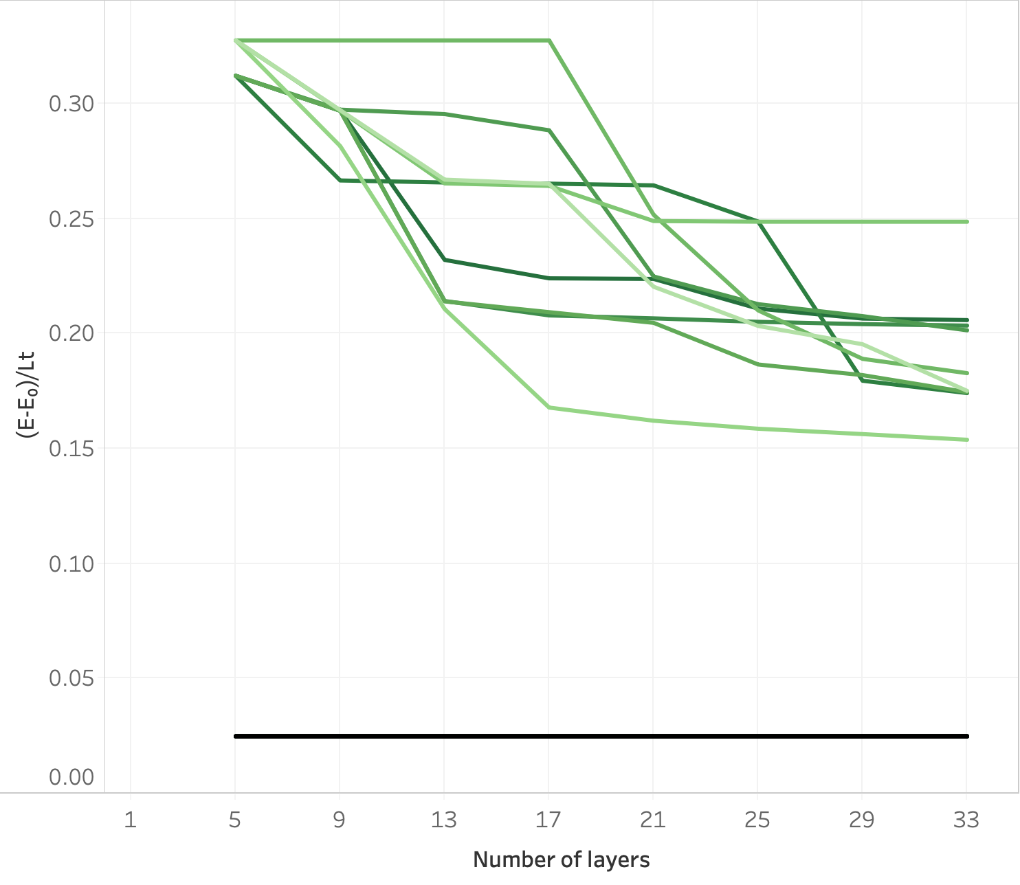
To study the sensitivity of the VQE optimization to the random initialization of parameters in our layer-by-layer strategy, we performed 9 VQE simulations with randomly chosen initial parameters of the chain on a grid of qubits with horizontal ordering. As observed in Fig. 10, the best value achieved for the energy density deviation is 0.15, with most of the final values for different calculations concentrating around 0.18. This result highlights how the layer-by-layer strategy consistently decreases the energy throughout the optimization, achieving roughly the same results for all runs. Therefore, the fact that the error expected for the ground state energy is not attained is attributed to the limited circuit depth imposed on the ansatz. In contrast, most of the simulations for the chain and smaller systems converged within an error of 0.02 from the exact value despite slight differences in the convergence paths for different runs.
V Discussion

We have proposed a benchmark to characterize the ability of near-term quantum processors to simulate a fermionic system with the variational quantum eigensolver. Our application benchmark utilizes the 1D FHM as the test Hamiltonian, providing an effective fermionic length that quantifies the size of fermionic systems that can be studied in a device for a particular choice of variational ansatz. Our benchmark is scalable in the sense that it requires a modest number of measurements and the knowledge of the exact energy of the 1D FHM in the thermodynamic limit, which can be obtained analytically. We provide a concrete implementation proposal of the benchmark for the Sycamore processor Arute et al. 2019 and demonstrate its viability through numerical experiments. Our results show that the hypothesized behavior of the benchmark is recovered when considering variational circuits with bounded depth as a way to emulate the effect of noise.
An important aspect of our benchmark is its runtime requirement, which depends on the number of measurements utilized in the VQE energy estimation process. The sampling rate is independent of the number of qubits and is inversely proportional to the depth of the circuit on the experimental device. On the Sycamore device, samples are obtained at a rate of 5 kHz. Assuming that measurements are distributed according to an optimal operator averaging strategy Rubin et al. 2018, and taking advantage of grouping of co-measurable terms, we have estimated that reaching an accuracy of for the energy density of the chain would require about 9 seconds of sampling, while an accuracy of would take around 15 minutes. Here, we also assume that covariances among the terms in the same group average to zero, which in our experience results in a slight overestimation of the number of necessary measurements. As pointed out in Section II.2, the number of measurements, and therefore estimation times, are expected to decrease for maintaining the same error in estimating energy per site as the chain gets longer. This analysis indicates that estimating the required quantities for the benchmark is practical on existing quantum devices.
A potential obstacle to the scalability of our scheme lies in the number of function evaluations required for training the ansatz, which is not in the scope of this paper but for which we recognize ample opportunities for further improvements. A significant improvement of the training method could involve a more advanced initialization method of the parameters using matrix product states Ran 2019 and tensor networks Biamonte and Bergholm 2017 for arbitrary universal hardware-efficient ansatzes. A simpler training heuristic could also involve using adiabatic-assisted VQE Garcia-Saez and Latorre 2018 to construct increasingly longer chains of the FHM. Similarly, characterizing the impact of different device errors in the VQE optimization, and simulations of the benchmark under more realistic noise conditions are left to future work.
Another possible avenue for improvement relates to the fermionic nature of the device ansatz as described in Section III.2. As shown in Ref. Dallaire-Demers et al. 2019, a circuit consisting of nearest-neighbor iSWAP gates corresponds to a basis rotation realized by time evolution under a free-fermion Hamiltonian Terhal and DiVincenzo 2002. Therefore one could improve the training by first using classical mean-field calculations to prepare the optimal Gaussian state using a basis rotation, and proceed to add parameterized ZZ gates and non-nearest-neighbor iSWAP gates for refining the ansatz into the space of non-Gaussian states Dallaire-Demers et al. 2019. Once the benchmark has been executed on a device and found useful for a given application of VQE, a more refined training method would be the one described in Appendix B. This method has the advantage that it cannot yield a state with higher energy than the mean-field state, which can be computed efficiently on a classical computer but it generally requires more measurements to converge than the 1D FHM benchmark.
Future research will explore the error resilience Sharma et al. 2019 of the proposed ansatz. In particular, we hypothesize that just as some coherent errors can be mitigated by a parameterized quantum circuit, the incorporation of auxiliary qubits could mitigate some incoherent errors as they allow for the implementation of parameterized quantum channels. In this case, the auxiliary qubits serve effectively as a bath such as the entropy generated by incoherent processes can be dissipated through them, opening a potential avenue to improve the performance of VQE. The study of this hypothesis as well as the interplay of the proposed benchmark with previously proposed error mitigation techniques Temme et al. 2017; Endo et al. 2018; Kandala et al. 2019; McArdle et al. 2018 are left for future work.
Another research direction is the use of the VQE ansatz and optimization strategy proposed in this paper in the study of more complex fermionic simulation problems. For instance, as the computation of the Green′s function of the one-dimensional FHM is difficult in practice with the Bethe ansatz, we propose using subspace-search VQE to measure the single-particle Green′s function of the Hubbard model as is done in Endo et al. 2019. Also, once a one-dimensional FHM chain can be converged on a quantum processor, we propose using adiabatic-assisted VQE to prepare the ground state of more complicated systems like the two-dimensional FHM. Furthermore, it would be possible to try optimizing a instance of the FHM by taking advantage of the full size of the Sycamore chip. This would be a step on the path to concrete applications of quantum computing technologies.
Finally, it should be possible to design hardware efficient fermionic ansatzes for other quantum computing architectures such as ion traps. In principle, this ansatz could be realized using native gates, such as the Mølmer-Sørensen gate, and a trap architecture that allows for the execution of a number of simultaneous two-qubit gates that scales with the number of qubits.
Acknowledgement
PLDD proposed the theoretical aspects of the benchmark. JG, JR, NTB and MS composed the Orquestra workflows to generate the simulation data. MS and NTB executed the workflows and analyzed the results. PLDD, JR and YC wrote the paper. The authors thank Peter Johnson for inspiration of the advanced training method as well as Max Radin, Borja Peropadre, Morten Kjaergaard and Gabriel Samach for helpful discussions and insights, and Maria Genckel for the much improved presentation of the workflow diagram. We also thank Jonny Olson for proof-reading and fine-tuning the final manuscript.
References
- Preskill (2018) J. Preskill, Quantum computing in the NISQ era and beyond, Quantum 2, 79 (2018).
- Peruzzo et al. (2014) A. Peruzzo, J. McClean, P. Shadbolt, M.-H. Yung, X.-Q. Zhou, P. J. Love, A. Aspuru-Guzik, and J. L. O′brien, A variational eigenvalue solver on a photonic quantum processor, Nat. Commun. 5, 4213 (2014).
- Wecker et al. (2015) D. Wecker, M. B. Hastings, and M. Troyer, Progress towards practical quantum variational algorithms, Phys. Rev. A 92, 10.1103/physreva.92.042303 (2015).
- McClean et al. (2016) J. R. McClean, J. Romero, R. Babbush, and A. Aspuru-Guzik, The theory of variational hybrid quantum-classical algorithms, New J. Phys. 18, 023023 (2016).
- Kandala et al. (2017) A. Kandala, A. Mezzacapo, K. Temme, M. Takita, M. Brink, J. M. Chow, and J. M. Gambetta, Hardware-efficient variational quantum eigensolver for small molecules and quantum magnets, Nature 549, 242 (2017).
- Fontalvo et al. (2018) J. R. Fontalvo, R. Babbush, J. McClean, C. Hempel, P. J. Love, and A. Aspuru-Guzik, Strategies for quantum computing molecular energies using the unitary coupled cluster ansatz, Quantum Sci. Technol. 4, 14008 (2018).
- Dallaire-Demers et al. (2019) P.-L. Dallaire-Demers, J. Romero, L. Veis, S. Sim, and A. Aspuru-Guzik, Low-depth circuit ansatz for preparing correlated fermionic states on a quantum computer, Quantum Sci. Technol. 4, 045005 (2019).
- McArdle et al. (2019) S. McArdle, T. Jones, S. Endo, Y. Li, S. C. Benjamin, and X. Yuan, Variational ansatz-based quantum simulation of imaginary time evolution, npj Quantum Inf. 5, 10.1038/s41534-019-0187-2 (2019).
- Yuan et al. (2019) X. Yuan, S. Endo, Q. Zhao, Y. Li, and S. C. Benjamin, Theory of variational quantum simulation, Quantum 3, 191 (2019).
- Farhi et al. (2014) E. Farhi, J. Goldstone, and S. Gutmann, A quantum approximate optimization algorithm, MIT-CTP/4610 (2014).
- Zhou et al. (2018) L. Zhou, S.-T. Wang, S. Choi, H. Pichler, and M. D. Lukin, Quantum approximate optimization algorithm: Performance, mechanism, and implementation on near-term devices, arXiv:1812.01041 [quant-ph] (2018).
- Schuld et al. (2018) M. Schuld, A. Bocharov, K. Svore, and N. Wiebe, Circuit-centric quantum classifiers (2018), arXiv:1804.00633 [quant-ph] .
- Dallaire-Demers and Killoran (2018) P.-L. Dallaire-Demers and N. Killoran, Quantum generative adversarial networks, Phys. Rev. A 98, 012324 (2018).
- Havlíček et al. (2019) V. Havlíček, A. D. Córcoles, K. Temme, A. W. Harrow, A. Kandala, J. M. Chow, and J. M. Gambetta, Supervised learning with quantum-enhanced feature spaces, Nature 567, 209 (2019).
- Schuld and Killoran (2019) M. Schuld and N. Killoran, Quantum machine learning in feature hilbert spaces, Phys. Rev. Lett. 122, 10.1103/physrevlett.122.040504 (2019).
- Benedetti et al. (2019) M. Benedetti, D. Garcia-Pintos, O. Perdomo, V. Leyton-Ortega, Y. Nam, and A. Perdomo-Ortiz, A generative modeling approach for benchmarking and training shallow quantum circuits, npj Quantum Inf. 5, 10.1038/s41534-019-0157-8 (2019).
- Xu et al. (2019) X. Xu, J. Sun, S. Endo, Y. Li, S. C. Benjamin, and X. Yuan, Variational algorithms for linear algebra (2019), arXiv:1909.03898 [quant-ph] .
- Bravo-Prieto et al. (2019) C. Bravo-Prieto, R. LaRose, M. Cerezo, Y. Subasi, L. Cincio, and P. J. Coles, Variational quantum linear solver: A hybrid algorithm for linear systems (2019), arXiv:1909.05820 [quant-ph] .
- Huang et al. (2019) H.-Y. Huang, K. Bharti, and P. Rebentrost, Near-term quantum algorithms for linear systems of equations (2019), arXiv:1909.07344 [quant-ph] .
- Proctor et al. (2017) T. Proctor, K. Rudinger, K. Young, M. Sarovar, and R. Blume-Kohout, What randomized benchmarking actually measures, Phys. Rev. Lett. 119, 10.1103/physrevlett.119.130502 (2017).
- Cross et al. (2019) A. W. Cross, L. S. Bishop, S. Sheldon, P. D. Nation, and J. M. Gambetta, Validating quantum computers using randomized model circuits, Phys. Rev. A 100, 10.1103/physreva.100.032328 (2019).
- Arute et al. (2019) F. Arute, K. Arya, R. Babbush, D. Bacon, J. C. Bardin, R. Barends, R. Biswas, S. Boixo, F. G. Brandao, D. A. Buell, et al., Quantum supremacy using a programmable superconducting processor, Nature 574, 505 (2019).
- Foxen et al. (2020) B. Foxen, C. Neill, A. Dunsworth, P. Roushan, B. Chiaro, A. Megrant, J. Kelly, Z. Chen, K. Satzinger, R. Barends, et al., Demonstrating a continuous set of two-qubit gates for near-term quantum algorithms, arXiv preprint arXiv:2001.08343 (2020).
- Brod and Childs (2014) D. J. Brod and A. M. Childs, The computational power of matchgates and the xy interaction on arbitrary graphs, Quantum Inf. Comput. 14, 10.26421/qic14.11-12 (2014).
- Terhal and DiVincenzo (2002) B. M. Terhal and D. P. DiVincenzo, Classical simulation of noninteracting-fermion quantum circuits, Phys. Rev. A 65, 032325 (2002).
- Jozsa and Miyake (2008) R. Jozsa and A. Miyake, Matchgates and classical simulation of quantum circuits, Proceedings of the Royal Society A: Mathematical, Physical and Engineering Sciences 464, 3089 (2008).
- Bedürftig and Frahm (1997) G. Bedürftig and H. Frahm, Spectrum of boundary states in the open hubbard chain, J. Phys. A: Math. Gen. 30, 4139 (1997).
- Lieb and Wu (2003) E. H. Lieb and F. Wu, The one-dimensional hubbard model: a reminiscence, Physica A 321, 1 (2003).
- Balzer et al. (2008) M. Balzer, W. Hanke, and M. Potthoff, Mott transition in one dimension: Benchmarking dynamical cluster approaches, Phys. Rev. B 77, 045133 (2008).
- Essler et al. (2005) F. H. Essler, H. Frahm, F. Göhmann, A. Klümper, and V. E. Korepin, The one-dimensional Hubbard model (Cambridge University Press, 2005).
- Cao et al. (2019) Y. Cao, J. Romero, J. P. Olson, M. Degroote, P. D. Johnson, M. Kieferová, I. D. Kivlichan, T. Menke, B. Peropadre, N. P. Sawaya, et al., Quantum chemistry in the age of quantum computing, Chem. Rev. 119, 10856 (2019).
- Kivlichan et al. (2018) I. D. Kivlichan, J. McClean, N. Wiebe, C. Gidney, A. Aspuru-Guzik, G. K.-L. Chan, and R. Babbush, Quantum simulation of electronic structure with linear depth and connectivity, Phys. Rev. Lett. 120, 110501 (2018).
- Jiang et al. (2018) Z. Jiang, K. J. Sung, K. Kechedzhi, V. N. Smelyanskiy, and S. Boixo, Quantum algorithms to simulate many-body physics of correlated fermions, Phys. Rev. Applied 9, 044036 (2018).
- Pino et al. (2020) J. M. Pino, J. M. Dreiling, C. Figgatt, J. P. Gaebler, S. A. Moses, C. H. Baldwin, M. Foss-Feig, D. Hayes, K. Mayer, C. Ryan-Anderson, and B. Neyenhuis, Demonstration of the QCCD trapped-ion quantum computer architecture (2020).
- McClean et al. (2018) J. R. McClean, S. Boixo, V. N. Smelyanskiy, R. Babbush, and H. Neven, Barren plateaus in quantum neural network training landscapes, Nat. Commun. 9, 1 (2018).
- Cerezo et al. (2020) M. Cerezo, A. Sone, T. Volkoff, L. Cincio, and P. J. Coles, Cost-function-dependent barren plateaus in shallow quantum neural networks, arXiv preprint arXiv:2001.00550 (2020).
- Nielsen and Chuang (2002) M. A. Nielsen and I. Chuang, Quantum computation and quantum information (AAPT, 2002).
- (38) Orquestra. http://orquestra.io/.
- Guerreschi et al. (2020) G. G. Guerreschi, J. Hogaboam, F. Baruffa, and N. Sawaya, Intel quantum simulator: A cloud-ready high-performance simulator of quantum circuits, arXiv preprint arXiv:2001.10554 (2020).
- Kraft (1988) D. Kraft, A software package for sequential quadratic programming, DFVLR-FB , 88 (1988).
- Kraft (1994) D. Kraft, Algorithm 733: Tomp-fortran modules for optimal control calculations, ACM Trans. Math. Software 20, 262 (1994).
- Rubin et al. (2018) N. C. Rubin, R. Babbush, and J. McClean, Application of fermionic marginal constraints to hybrid quantum algorithms, New J. Phys. 20, 053020 (2018), arXiv:1801.03524 [quant-ph] .
- Ran (2019) S.-J. Ran, Efficient encoding of matrix product states into quantum circuits of one-and two-qubit gates, arXiv preprint arXiv:1908.07958 (2019).
- Biamonte and Bergholm (2017) J. Biamonte and V. Bergholm, Tensor networks in a nutshell, arXiv preprint arXiv:1708.00006 (2017).
- Garcia-Saez and Latorre (2018) A. Garcia-Saez and J. Latorre, Addressing hard classical problems with adiabatically assisted variational quantum eigensolvers, arXiv preprint arXiv:1806.02287 (2018).
- Sharma et al. (2019) K. Sharma, S. Khatri, M. Cerezo, and P. J. Coles, Noise resilience of variational quantum compiling, arXiv preprint arXiv:1908.04416 (2019).
- Temme et al. (2017) K. Temme, S. Bravyi, and J. M. Gambetta, Error mitigation for short-depth quantum circuits, Phys. Rev. Lett. 119, 180509 (2017).
- Endo et al. (2018) S. Endo, S. C. Benjamin, and Y. Li, Practical quantum error mitigation for near-future applications, Phys. Rev. X 8, 031027 (2018).
- Kandala et al. (2019) A. Kandala, K. Temme, A. D. Córcoles, A. Mezzacapo, J. M. Chow, and J. M. Gambetta, Error mitigation extends the computational reach of a noisy quantum processor, Nature 567, 491 (2019).
- McArdle et al. (2018) S. McArdle, X. Yuan, and S. Benjamin, Error mitigated quantum computational chemistry, arXiv preprint arXiv:1807.02467 (2018).
- Endo et al. (2019) S. Endo, I. Kurata, and Y. O. Nakagawa, Calculation of the green’s function on near-term quantum computers, arXiv preprint arXiv:1909.12250 (2019).
- Valiant (2002) L. G. Valiant, Quantum circuits that can be simulated classically in polynomial time, SIAM J. Comput. 31, 1229 (2002).
- Valiant (2008) L. G. Valiant, Holographic algorithms, SIAM J. Comput. 37, 1565 (2008).
- Schuld et al. (2019) M. Schuld, V. Bergholm, C. Gogolin, J. Izaac, and N. Killoran, Evaluating analytic gradients on quantum hardware, Phys. Rev. A 99, 032331 (2019).
Appendix A Fermionic character of the ansatz
Here we present a short review of the formalism of fermionic gaussian transformations and their correspondence to networks of nearest-neighbor matchgates. For a more detailed treatment we refer to Terhal and DiVincenzo 2002; Jozsa and Miyake 2008. It is useful to use the real quadrature of the fermionic field which are the Majorana operators
| (6) |
In the diagonal basis of a quadratic fermionic Hamiltonian, a Slater determinant over spin orbitals can be constructed from the vacuum as a product of single particles
| (7) |
where the are the Williamson eigenvalues. In general, the density matrix of a fermionic gaussian state can always be represented in the form
| (8) |
A more compact notation is given by a covariance matrix whose elements can be computed as
| (9) |
This can be written in the diagonal form as
| (10) |
where is a rotation. Those rotations are Bogoliubov transformations in general and orbital rotations in the particular case where the number of particles is conserved.
We can now establish the connection to nearest-neighbor matchgates introduced by Valiant Valiant 2002; Valiant 2008. A general matchgate between two qubits is defined by
| (11) |
where and are SU(2) rotations with the same determinant . Nearest-neighbor matchgates acting on two qubits have six generators
| (12) |
which explicitly correspond to quadratic forms of Majorana operators after a Jordan-Wigner transformation. In general, a full network of matchgates can generate any rotation. A general rotation is parametrized by angles and can be implemented in linear circuit depth on a linear array of qubits Dallaire-Demers et al. 2019.
If is a circuit of nearest-neighbor matchgates, the holographic relation that translates the transformation from Hilbert space to a rotation in the space of fermionic operators is given by
| (13) |
Finally, the connection to fermionic gaussian transformation is established through quadratic fermionic Hamiltonian of the form
| (14) |
where is a real and antisymmetric matrix. A general Bogoliubov transformation in the space of fermionic ladder operators has the form .
Appendix B Advanced training method
The ansatz defined in Section III can be used for the general VQE procedure. In that case, we are interested to find a fermionic ground state which improves upon the mean field state which is classically efficient to compute. To maximize the use of the non-Gaussian resources contained in the quantum ansatz, it is best to offload all Gaussian transformations with a classical computer.
The full cost function for an ansatz that do not necessarily conserve the number of particles is given by
| (15) |
where is the state parametrized on the quantum computer and is the Hamiltonian represented in a basis which can be optimized variationally on a classical computer.
The general training method is a modified Newton procedure where at each step we compute the cost function At each step, we must compute the cost function . The parameters are updated with the rule
| (16) |
where and are computed from
| (17) |
We define the global gradient operator as and the Hessian as . The gradients can be measured as
| (18) |
where . The second order derivative have the form
| (19) |
The first and second derivatives with respect to can be measured with the parameter shift rule Schuld et al. 2019.