Alfnoor: A Retrieval Simulation of the Ariel Target List.

To study large samples of exoplanetary spectra, we built a new tool: Alfnoor. Alfnoor combines the highly flexible next generation retrieval code TauREx 3 with the ArielRad noise simulator to provide a unique framework dedicated to the study of exoplanetary populations with Ariel.

TauREx 3 (Al-Refaie et al. 2019) is the new version of TauREx (Waldmann et al. 2015a; Waldmann et al. 2015b). This complete rewrite takes the form of a library and is designed to make customisation and external code integration easy. It uses the highly accurate line-lists from the ExoMol (Tennyson et al. 2016), HITRAN (Rothman & Gordon 2014) and HITEMP (Gordon et al. 2016) databases to build forward and retrieval models. A large number of options are available in terms of forward models (transmission, emission), chemical profiles (constant as a function of pressure, two-layer, equilibrium chemistry), temperature profiles (isothermal, NPoints, Guillot 2010) and cloud parameterisations (Grey, Lee et al. 2013,Bohren & Huffman 2008).

ArielRad (Mugnai et al. 2020b) estimates Ariel performances to observe a certain target when stellar, planetary and orbital parameters are specified. It also calculates the required number of observations to match the requirements for each of Ariel’s tiers (Edwards et al. 2019a). In our study we focused on Tier-2 observations, which is the core of the mission, and aims at characterising the key chemical species, thermal structure and the cloud properties of the selected atmospheres. Ariel observations are expected to cover the wavelengths from 0.5$\mu m$ to 7.8$\mu m$. The telescope has 3 photometers: a Visible Photometer (VISPhot) and two Fine Guidance Sensors (FGS1 and FGS2) that are also used for the observations. The telescope also has two spectrometers: the Near Infrared Spectrometer (NIRSpec) and the Ariel Infrared Spectrometer (AIRS). The resolution of the spectrometers is adapted to the Tier levels. A description of the resolution achieved for each Tier can be found in Tinetti et al. 2018, Edwards et al. 2019a and Mugnai et al. 2020b. It is summarised in Table 1.

The function Alfnoor-forward simulated high-resolution transit spectra with TauREx 3 for all the targets. Next it called ArielRad to calculate the Ariel error bars, wavelength bins and the number of required observations to reach Tier-2 performances for all the targets. The function alfnoor-inverse took the Tier-2 spectra generated by alfnoor-forward and performed atmospheric retrievals using TauREx 3 in fitting mode.

Tier 1 observations are studied in detail in Mugnai et al. 2020a. Our sample of planets consists of the 146 planets observed in transit at Tier 2 from the Mission Reference Sample presented in Edwards et al. 2019a. Of these planets, 14 of them qualify for observations in Tier 3. The simulated planets are built to represent the entire parameter space. In our sample 20 planets have radius smaller than 2 R_E, 29 are between 2 - 5 R_E and 97 have radius $>5$ R_E. For a more detailed description of the methodology used to build this target list, we refer the reader to Edwards et al. 2019a. Future studies will concentrate on eclipse observations and / or secondary atmospheres.

In all the models, the atmosphere is composed of H₂ and He with a ratio He/H₂ = 0.17. For the trace-gases, the list and sources of the opacities used in this paper are presented in Table 2. Collision Induced Absorption for H₂-H₂ and H₂-He and Rayleigh scattering are included. For the retrievals, unless specified otherwise, we used the same assumptions: mixing ratios constant with pressure, temperature constant with pressure, grey opaque clouds. While temperature variations with altitude are crucial for eclipse observations, in the case of transmission spectra, most studies assume isothermal temperature profiles. This is justified by the narrow wavelength coverage and signal-to-noise in available observations (with the Hubble Space Telescope) which is not allowing to probe large pressure regions in the planet atmosphere. The temperature variations in transmission act as a second order parameter and the spectrum is most sensitive to the mean temperature value, which directly appear in the scale height. However, Barstow et al. 2012, Rocchetto et al. 2016 and Changeat et al. 2019 highlighted the impact of temperature variations for high signal-to-noise and broad wavelength coverage cases, indicating that JWST and Ariel would be able to retrieve more complex temperature structures from transit spectra. As this study focuses on the capabilities of Ariel to recover chemical species, we do not investigate further the impact of non-isothermal temperature structures. We however note that this assumption could introduce biases to our results. Parameters that are traditionally determined using external methods are fixed to the true values: e.g. stellar radius, planetary mass and He/H₂ ratio. The list of free parameters along with the priors used are described in Table 3

In this study, we aim to explore two particular aspects of the Ariel mission:

1. 1.

   the ability of Ariel to detect molecular species and the detection limits for these molecules in the context of cloudy primary atmospheres observed in transit. This task can be easily achieved by performing retrievals on an unbiased dataset of planets where the atmospheric composition is randomised and by assessing the cases that have been successfully recovered.

2. 2.

   the ability of Ariel to reveal chemical trends in exoplanet populations. To assess this possibility, a biased sample can be used as input where an artificial trend is introduced.

We describe below the actual implementation of this plan.

1. 1.

   Unbiased sample. We built the forward model by using the stellar and planetary basic parameters from Edwards et al. 2019a for the Ariel Target list. We randomised the chemistry, temperature and cloud parameters so that a unique set of these parameters is adopted for each planet of each sample. For the chemistry, we considered constant profiles with pressure for the mixing ratios of H₂O, CH₄, CO, CO₂ and NH₃ and chose a random abundance in logarithmic scale from $10^{-7}$ to $10^{-2}$. For clouds, we generated grey opaque clouds with random top pressures varying in log-scale from 10 bar (equivalent to no clouds) to $10^{-3}$ bar. Finally, the atmospheric temperatures were also randomly generated and allowed to assume values between $0.7\times T_{eff}$ and $1.05\times T_{eff}$, where $T_{eff}$ is the effective temperature in the Ariel target list of Edwards et al. 2019a. The temperature was consciously selected biased towards lower values to account for differences between effective temperature and the terminator temperature (Caldas et al. 2019). We repeated the generation of the observed spectra twice to build ‘un-scattered’ and ‘scattered’ datasets. In the un-scattered set, we conserve the theoretical simulated spectra as-is. As scatter generally arises from the random realisation of observations, we apply a Gaussian scatter to a second dataset using the true value as mean and the simulated noise as variance. This scattered dataset better describes what would be obtained in an actual observation by the telescope but cannot be used to characterise retrieval biases as ‘unfortunate’ runs could lead to large discrepancies between true and retrieved values (Feng et al. 2018; Changeat et al. 2019). Unscattered spectra are more suitable for the study of retrieval biases and intrinsic correlations between the atmospheric parameters (Feng et al. 2018). On the opposite, scattered spectra can inform us on the stability and the redundancy in the information content of Ariel spectra. Previous studies have used both types to simulate observations by future telescopes (Barstow et al. 2012; Tinetti et al. 2015; Feng et al. 2016; Rocchetto et al. 2016; Mollière et al. 2017; Batalha et al. 2017; Tinetti et al. 2018; Blumenthal et al. 2018; Feng et al. 2018; Edwards et al. 2019b; Changeat et al. 2019; Lustig-Yaeger et al. 2019; Changeat et al. 2020). Feng et al. 2018 results predicted that the retrieved uncertainties should be similar in both scattered and un-scattered runs but that the retrieved mean could be different. Here, we use our two datasets to investigate these predictions keeping in mind that if Ariel spectra contain enough information content redundancy, we should not see large differences in the retrieved mean values.

2. 2.

   Biased samples. We imposed first a linear relationship between the logarithmic abundance of water and the temperature. We enacted this correlation water-temperature by requiring a mixing ratio of $10^{-4}$ for an effective temperature of 1000K and $10^{-3}$ for an effective temperature of 2000K.

   We then tried a more realistic example where the atmospheres were assumed to be in chemical equilibrium and simulated accordingly the chemical abundances and profiles (Agúndez et al. 2012). We used the same solar C/O ratio and metallicity for all the planets in the sample. To recover the input profiles, we used in the retrievals both free, constant with altitude chemical profiles and profiles which are forced to follow chemical equilibrium prescriptions. We did not test the entire sample with the two-layer chemistry retrieval scheme as presented in Changeat et al. 2019, but we have run an example to show the expected improvements of this scheme over the pressure constant chemical profiles.

We show in Figure 1 both the observed and retrieved spectra for a subset of the simulated Ariel Tier-2 observations, along with the correlation map between water abundance and temperature with their 1$\sigma$ uncertainties. The distance between the true and the retrieved value is visualised by the colour of the point. The retrieved parameters are represented by the median chemical or temperature profiles weighted by the contribution function. The contribution function is defined as the wavelengths averaged variations of the optical depth with pressure. This choice ensures that the values reported well reflect the conditions in the atmospheric regions probed by observations. In order to better visualise the Ariel detection limits in Tier 2, we also provide complementary plots of the retrieved abundances versus their true values for each molecule. The H₂O map is presented in Figure 2.

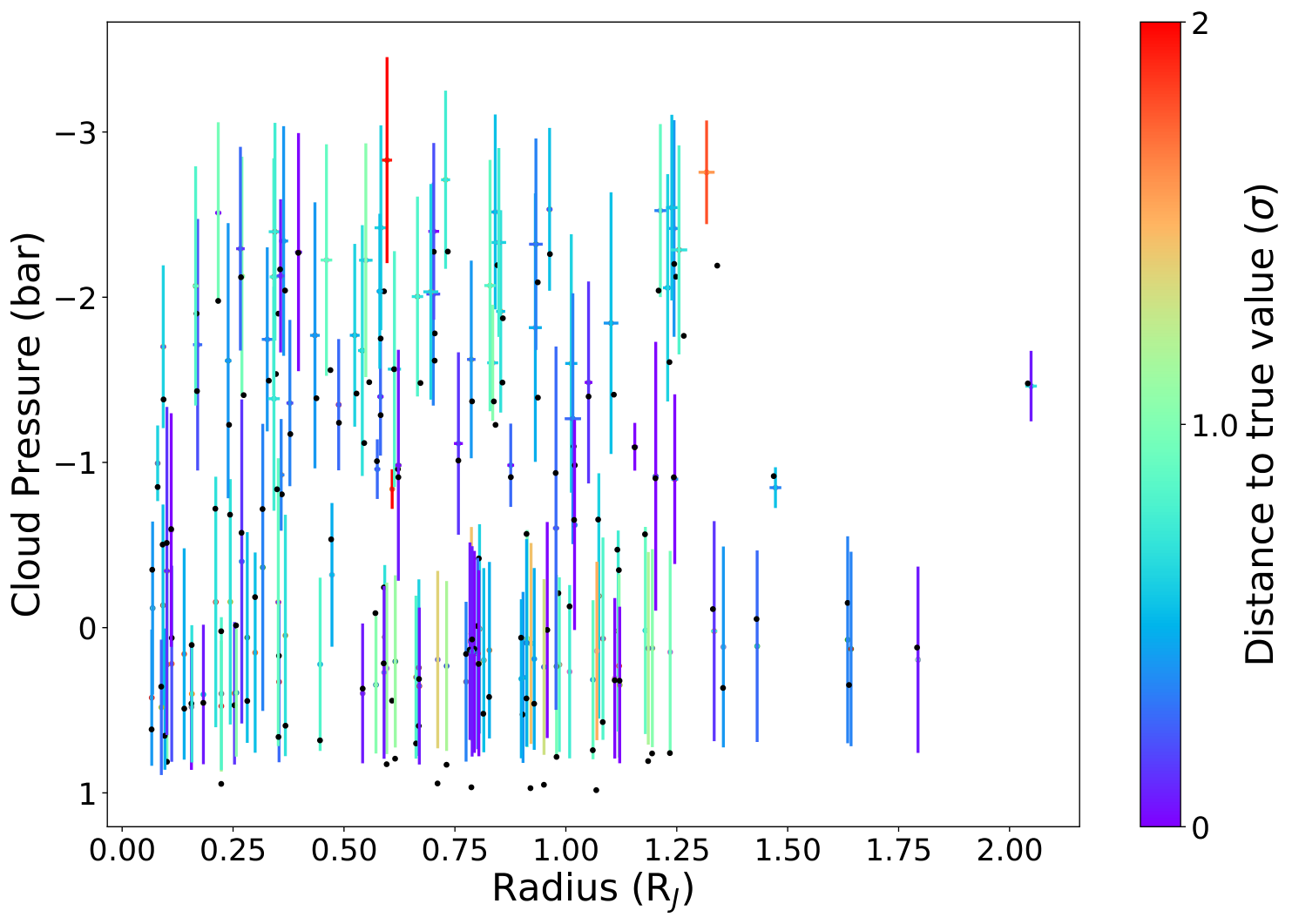
The water-temperature map in Figure 1 clearly shows that our unbiased population is randomly spread in the parameter space, as expected. The retrieved temperature is very precise across the whole parameter space, showcasing the ability of Ariel Tier-2 to study a wide range of planets. It also illustrates that the retrieved values are mostly accurate for water abundances higher than $10^{-6}$: with the exception of a few cases, the retrieved values for water and temperature fall well within the 1$\sigma$ error bars (blue to green in the colour scale). We notice for water a rapid change in the posteriors for abundances smaller than $10^{-5}$, marked by large error bars on the left side of the plot. Indeed, when the abundance is too low, the retrievals are not able to distinguish well the features and provide only upper limits. This is an expected behaviour and an indication of the Ariel detection limit for our sample of planets. This exercise was repeated for other molecules to assess Ariel ability to detect different sets of molecules in Tier-2 mode. Other temperature-molecule maps, as well as the radius-clouds map, are reported in Appendix (Figures 8, 9, 10, 11, 12).

The detection limits are best visualised in the retrieved versus true abundances (see Figure 2). In the same Figure, we also show the retrieved uncertainties versus input abundances as this allows us to distinguish 3 regimes. The first regime corresponds to low abundances where molecular detections are not possible: for example, between 10^-7 and 10^-6 for water no detections seem possible with Ariel. Other molecules are presented in Figures 13: CH₄; Figure 14: CO; Figure 15: CO₂ and Figure 16: NH₃. It is interesting to note that when the molecules are not detected, the retrieved errors ($\sigma$) are dominated by the size of the priors and the location of the detection limit: for water no-detection errors are between 2 and 4 orders of magnitude. The second regime for intermediate abundances displays a mix between successful detections and lack of evidence for the molecules. This corresponds to the region with large ranges in the retrieved errors (between 10^-6 and 10^-5 for water). In general, this variability is due to the other constituents in the planet that are susceptible to mask the signal of interest (e.g: clouds, other molecules). Finally, for the highest abundances, the retrieved uncertainties are low (less than 1 order of magnitude in the mixing ratios), which indicate that these abundances are always retrieved, regardless of the other constituents in the atmosphere.

Additionally, the map exploring the correlation between planetary radius and cloud top pressure shows that Ariel can separate well these parameters, most likely thanks to the FGS optical channels.

We repeated the same experiment with the second run composed of ’scattered’ spectra. Each planet is simulated with a new set of randomised parameters. As previously stated, the observed values of the transit depth are assumed to follow a normal distribution (the mean is the simulated transit depth and the standard deviation is the instrumental noise), which better reproduces a real observation. Figure 3 shows the water-temperature map. The other chemical parameters are reported in Appendix (Figures 8, 9, 10, 11, 12). From the analysis of the scattered spectra, we appreciate that the scattering of the data points around their true value does not necessary introduce biases in Ariel Tier-2 retrieval studies. Indeed, this result, which has already been explored in Feng et al. 2018; Changeat et al. 2019, naturally arises from the redundancy of the information relative to each molecule in the Ariel spectra and the fact that in most cases N repeated observations are needed to obtain Tier-2 requirements, therefore reducing by $1/\sqrt{N}$ the scattering amplitude around their true value. Feng et al. 2018 highlighted that, to avoid potential biases arising from individual noise instances, one would essentially have to produce multiple retrievals with different noise instances and average the obtained results. As this was not computationally feasible, they chose not to scatter the spectra and use the true value as an approximation, stating that the shape of the posteriors would be accurate but that the position may be optimistically centred. For Ariel Tier-2 observations, the information content of the spectra is redundant enough to ensure that the retrieved values are not affected by this phenomenon and these are mostly centred around the true value in both scattered and non-scattered scenarios. For all molecules, we find that the correlation maps are very similar in both cases and the detection limits remain unchanged from the non-scattered runs. For the clouds, however, we note an overall increase in the distance to the true value (see correlation map in Appendix Figure 12). We note that in the simulations presented here, we considered fully opaque grey cloud cover, which is essentially the worst case scenario as no cloud features are detectable and it is well known to be degenerate with radius (Changeat et al. 2020). More realistic cloud simulations will be considered in a future paper to test more thoroughly this case.

We summarise in Table 4 the approximate detection limits for each molecule considered. These represent the regions where our retrieval analysis have been able to extract constraints on the given atmospheric constituents. The stated detection limit corresponds to the lowest value that was successfully recovered with less than 1 order of magnitude uncertainties. As seen before, 3 regions of the parameter space can be identified: region 1 with no possible detections of the molecule, region 2 with detections depending on the other atmospheric properties and region 3 where the molecule is always detected. This means the stated values do not represent a guaranty of detection, but rather the lowest limit we can hope to detect the molecule. In addition, we plot the contribution of each molecule individually in Figure 17 (each spectrum only contains 10^-5 of the considered molecule) to show the features span by each molecule. In general, Ariel Tier-2 spectra should enable molecular detections down to mixing ratios of $10^{-6}$. In our simulations, only CO appears to be difficult to detect at abundances smaller than $10^{-4}$. CO presents two features that are overlapping with CO₂ at 4.5$\mu$m and with CH₄ at 2.5$\mu$m and are relatively weak. In a real scenario (equilibrium chemistry), we believe CO could be more easily distinguishable as our unbiased assumption underestimates the CO abundance and overestimates the CO₂ abundance by design (Agúndez et al. 2012; Venot et al. 2012; Venot & Agúndez 2015). We also note that H₂O and CH₄ have a large number of anti-correlated features, which may give rise to more featureless spectra when the two molecules are present. For all parameters, Ariel Tier-2 spectra provide accurate and precise estimates, as most of the retrieved error bars are less than 1-sigma away from the true value. This statement applies to both non-scattered and scattered spectra.

For completeness, we performed additional retrievals for 14 benchmark planets in Tier-3 mode (Edwards et al. 2019a). The benchmark planets achieve a high signal-to-noise ratio in a very limited number of transits and are re-observed at different times to allow for temporal and spatial variability studies. In the examples presented here, we combined five transit observations to reach the required signal-to-noise for Tier-3 (Edwards et al. 2019a; Tinetti et al. 2018). The retrievals were performed on the scattered spectra and are illustrated in Figure 4. The retrieval maps for the 14 Ariel Tier-3 cases are reported in Appendix (Figures 18, 19, 20) and the molecular detection limits in Table 4. The detection limit for Ariel Tier-3 spectra is very low, typically mixing ratios equal or smaller than $10^{-7}$ can be retrieved. Even CO at mixing ratios of $\sim 10^{-6}$ appears to be detectable. Due to the limited number of studied cases, the Tier-3 detection limits reported here should be taken with caution and will be refined in a separate paper dedicated to the study of Tier-3 planets.

When we imposed an arbitrary linear trend between the water abundance and the effective temperature, we obtained the water-temperature map shown in Figure 5. Here the imposed trend is easily recovered by our retrieval analysis. Both scattered and unscattered spectra allow to recover the imposed trend down to water abundances $\sim 10^{-6}$. In the scattered example, a few cases have larger departures from the true value compared to the non-scattered one but this does not affect the conclusions on the entire population. Additionally, we note that this analysis has been done without retrieval fine tuning.

When an equilibrium chemistry model was used for both the forward model and the retrievals, we obtained the water-temperature map shown in Figure 6, top, where the trend is very accurately and precisely recovered. Since the molecular abundances are varying with altitude, the values stated correspond to the average weighted by the atmospheric contribution function (the optical depth variations collapsed over wavelengths). Being the model generating and retrieving the data the same, this is an optimistic result, as we should not expect all atmospheres to satisfy the equilibrium chemistry assumption.

Also the free, constant with pressure chemistry retrievals (Figure 6, bottom) allow to recover the equilibrium chemistry trend. The retrieved parameters, however, have large distances from the true value, in some cases the offsets are greater than 2$\sigma$, meaning that the model confidently recovers a biased value. This behaviour, also present in other chemical species (see Appendix Figures 21, 22, 23, 24), is particularly noticeable for temperatures between 600K and 1100K: this region is known to exhibit large chemical gradients with altitude as the balance in the CH₄/CO reaction changes. These variations in the chemical profiles cannot be captured by our simplistic constant chemistry retrieval model.

It has been shown in Changeat et al. 2019 that Ariel and JWST will be sensitive to chemical vertical gradients and that retrieval techniques such as the two-layer parametrisation would be essential for the analysis of these next generation spectra.

We show in Figure (7) a comparison between the various retrieval techniques: the two-layer parametrisation (Changeat et al. 2019) well captures the departure of the methane profile from the constant with altitude case without strong prior assumptions, as opposed to the case of the equilibrium chemistry retrieval.

References

- Abel et al. (2011) Abel, M., Frommhold, L., Li, X., & Hunt, K. L. 2011, The Journal of Physical Chemistry A, 115, 6805
- Abel et al. (2012) —. 2012, The Journal of chemical physics, 136, 044319
- Agúndez et al. (2012) Agúndez, M., Venot, O., Iro, N., et al. 2012, Astronomy & Astrophysics, 548, A73. http://dx.doi.org/10.1051/0004-6361/201220365
- Al-Refaie et al. (2019) Al-Refaie, A. F., Changeat, Q., Waldmann, I. P., & Tinetti, G. 2019, TauREx III: A fast, dynamic and extendable framework for retrievals, , , arXiv:1912.07759
- Barstow et al. (2012) Barstow, J. K., Aigrain, S., Irwin, P. G. J., et al. 2012, On the potential of the EChO mission to characterise gas giant atmospheres, , , arXiv:1212.5020
- Barstow et al. (2016) Barstow, J. K., Aigrain, S., Irwin, P. G. J., & Sing, D. K. 2016, The Astrophysical Journal, 834, 50. http://dx.doi.org/10.3847/1538-4357/834/1/50
- Barton et al. (2017) Barton, E. J., Hill, C., Yurchenko, S. N., et al. 2017, Journal of Quantitative Spectroscopy and Radiative Transfer, 187, 453
- Batalha et al. (2017) Batalha, N. E., Mandell, A., Pontoppidan, K., et al. 2017, Publications of the Astronomical Society of the Pacific, 129, 064501. http://dx.doi.org/10.1088/1538-3873/aa65b0
- Bennett et al. (2018) Bennett, D. P., Akeson, R., Anderson, J., et al. 2018, The WFIRST Exoplanet Microlensing Survey, , , arXiv:1803.08564
- Beuzit et al. (2019) Beuzit, J. L., Vigan, A., Mouillet, D., et al. 2019, A&A, 631, A155
- Blumenthal et al. (2018) Blumenthal, S. D., Mandell, A. M., Hébrard, E., et al. 2018, The Astrophysical Journal, 853, 138. http://dx.doi.org/10.3847/1538-4357/aa9e51
- Bohren & Huffman (2008) Bohren, C. F., & Huffman, D. R. 2008, Absorption and scattering of light by small particles (John Wiley & Sons)
- Broeg et al. (2013) Broeg, C., Fortier, A., Ehrenreich, D., et al. 2013, in European Physical Journal Web of Conferences, Vol. 47, European Physical Journal Web of Conferences, 03005
- Caldas et al. (2019) Caldas, A., Leconte, J., Selsis, F., et al. 2019, Astronomy & Astrophysics, 623, A161
- Cameron et al. (2010) Cameron, A. C., Guenther, E., Smalley, B., et al. 2010, Monthly Notices of the Royal Astronomical Society, 407, 507–514. http://dx.doi.org/10.1111/j.1365-2966.2010.16922.x
- Changeat et al. (2019) Changeat, Q., Edwards, B., Waldmann, I. P., & Tinetti, G. 2019, The Astrophysical Journal, 886, 39. http://dx.doi.org/10.3847/1538-4357/ab4a14
- Changeat et al. (2020) Changeat, Q., Keyte, L., Waldmann, I. P., & Tinetti, G. 2020, The Astrophysical Journal, 896, 107. http://dx.doi.org/10.3847/1538-4357/ab8f8b
- Delrez et al. (2016) Delrez, L., Santerne, A., Almenara, J.-M., et al. 2016, Monthly Notices of the Royal Astronomical Society, 458, 4025–4043. http://dx.doi.org/10.1093/mnras/stw522
- Edwards et al. (2019a) Edwards, B., Mugnai, L., Tinetti, G., Pascale, E., & Sarkar, S. 2019a, AJ, 157, 242
- Edwards et al. (2019b) Edwards, B., Rice, M., Zingales, T., et al. 2019b, Experimental Astronomy, 47, 29
- Feng et al. (2016) Feng, Y. K., Line, M. R., Fortney, J. J., et al. 2016, The Astrophysical Journal, 829, 52. http://dx.doi.org/10.3847/0004-637X/829/1/52
- Feng et al. (2018) Feng, Y. K., Robinson, T. D., Fortney, J. J., et al. 2018, AJ, 155, 200
- Fletcher et al. (2018) Fletcher, L. N., Gustafsson, M., & Orton, G. S. 2018, The Astrophysical Journal Supplement Series, 235, 24
- Gaia Collaboration et al. (2016) Gaia Collaboration, Prusti, T., de Bruijne, J. H. J., et al. 2016, A&A, 595, A1
- Gardner et al. (2006) Gardner, J. P., Mather, J. C., Clampin, M., et al. 2006, Space Science Reviews, 123, 485–606. http://dx.doi.org/10.1007/s11214-006-8315-7
- Gaudi et al. (2017) Gaudi, B. S., Stassun, K. G., Collins, K. A., et al. 2017, Nature, 546, 514–518. http://dx.doi.org/10.1038/nature22392
- Gillon et al. (2016) Gillon, M., Jehin, E., Lederer, S. M., et al. 2016, Nature, 533, 221–224. http://dx.doi.org/10.1038/nature17448
- Gilmozzi & Spyromilio (2007) Gilmozzi, R., & Spyromilio, J. 2007, The Messenger, 127, 11
- Gordon et al. (2016) Gordon, I., Rothman, L. S., Wilzewski, J. S., et al. 2016, in AAS/Division for Planetary Sciences Meeting Abstracts, Vol. 48, AAS/Division for Planetary Sciences Meeting Abstracts #48, 421.13
- Guillot (2010) Guillot, T. 2010, A&A, 520, A27
- Hill et al. (2013) Hill, C., Yurchenko, S. N., & Tennyson, J. 2013, Icarus, 226, 1673
- Kass & Raftery (1995) Kass, R. E., & Raftery, A. E. 1995, Journal of the american statistical association, 90, 773
- Kreidberg et al. (2014) Kreidberg, L., Bean, J. L., Désert, J.-M., et al. 2014, The Astrophysical Journal, 793, L27. http://dx.doi.org/10.1088/2041-8205/793/2/L27
- Lee et al. (2013) Lee, J.-M., Heng, K., & Irwin, P. G. J. 2013, The Astrophysical Journal, 778, 97. https://doi.org/10.1088%2F0004-637x%2F778%2F2%2F97
- Li et al. (2015) Li, G., Gordon, I. E., Rothman, L. S., et al. 2015, The Astrophysical Journal Supplement Series, 216, 15
- Line et al. (2016) Line, M. R., Stevenson, K. B., Bean, J., et al. 2016, The Astronomical Journal, 152, 203. http://dx.doi.org/10.3847/0004-6256/152/6/203
- Lustig-Yaeger et al. (2019) Lustig-Yaeger, J., Meadows, V. S., & Lincowski, A. P. 2019, The Astronomical Journal, 158, 27. http://dx.doi.org/10.3847/1538-3881/ab21e0
- Macintosh et al. (2014) Macintosh, B., Graham, J. R., Ingraham, P., et al. 2014, Proceedings of the National Academy of Sciences, 111, 12661. https://www.pnas.org/content/111/35/12661
- Ment et al. (2019) Ment, K., Dittmann, J. A., Astudillo-Defru, N., et al. 2019, AJ, 157, 32
- Miller-Ricci Kempton et al. (2012) Miller-Ricci Kempton, E., Zahnle, K., & Fortney, J. J. 2012, ApJ, 745, 3
- Mollière et al. (2017) Mollière, P., van Boekel, R., Bouwman, J., et al. 2017, Astronomy and Astrophysics, 600, A10. http://dx.doi.org/10.1051/0004-6361/201629800
- Mugnai et al. (2020a) Mugnai, L., Changeat, Q., Al-Refaie, A., Tinetti, G., & Pascale, E. 2020a, in prep
- Mugnai et al. (2020b) Mugnai, L. V., Pascale, E., Edwards, B., Papageorgiou, A., & Sarkar, S. 2020b, Experimental Astronomy, arXiv:2009.07824
- Pepe et al. (2010) Pepe, F. A., Cristiani, S., Rebolo Lopez, R., et al. 2010, Society of Photo-Optical Instrumentation Engineers (SPIE) Conference Series, Vol. 7735, ESPRESSO: the Echelle spectrograph for rocky exoplanets and stable spectroscopic observations, 77350F
- Pinhas et al. (2019) Pinhas, A., Madhusudhan, N., Gandhi, S., & MacDonald, R. 2019, Monthly Notices of the Royal Astronomical Society, 482, 1485. http://dx.doi.org/10.1093/mnras/sty2544
- Polyansky et al. (2018) Polyansky, O. L., Kyuberis, A. A., Zobov, N. F., et al. 2018, Monthly Notices of the Royal Astronomical Society, 480, 2597
- Rauer et al. (2016) Rauer, H., Aerts, C., Cabrera, J., & PLATO Team. 2016, Astronomische Nachrichten, 337, 961
- Ricker et al. (2014) Ricker, G. R., Winn, J. N., Vanderspek, R., et al. 2014, Journal of Astronomical Telescopes, Instruments, and Systems, 1, 014003. http://dx.doi.org/10.1117/1.JATIS.1.1.014003
- Rocchetto et al. (2016) Rocchetto, M., Waldmann, I. P., Venot, O., Lagage, P. O., & Tinetti, G. 2016, ApJ, 833, 120
- Rothman et al. (2010) Rothman, L., Gordon, I., Barber, R., et al. 2010, Journal of Quantitative Spectroscopy and Radiative Transfer, 111, 2139
- Rothman & Gordon (2014) Rothman, L. S., & Gordon, I. E. 2014, in 13th International HITRAN Conference, June 2014, Cambridge, Massachusetts, USA
- Sing et al. (2015) Sing, D. K., Fortney, J. J., Nikolov, N., et al. 2015, Nature, 529, 59–62. http://dx.doi.org/10.1038/nature16068
- Skidmore (2015) Skidmore, W. 2015, Research in Astronomy and Astrophysics, 15, 1945–2140. http://dx.doi.org/10.1088/1674-4527/15/12/001
- Tennyson & Yurchenko (2012) Tennyson, J., & Yurchenko, S. N. 2012, Monthly Notices of the Royal Astronomical Society, 425, 21
- Tennyson et al. (2016) Tennyson, J., Yurchenko, S. N., Al-Refaie, A. F., et al. 2016, Journal of Molecular Spectroscopy, 327, 73 , new Visions of Spectroscopic Databases, Volume II. http://www.sciencedirect.com/science/article/pii/S0022285216300807
- Tinetti et al. (2015) Tinetti, G., Drossart, P., Eccleston, P., et al. 2015, Experimental Astronomy, 40, 329–391. http://dx.doi.org/10.1007/s10686-015-9484-8
- Tinetti et al. (2018) Tinetti, G., Drossart, P., Eccleston, P., et al. 2018, Experimental Astronomy, doi:10.1007/s10686-018-9598-x
- Tsiaras et al. (2019) Tsiaras, A., Waldmann, I. P., Tinetti, G., Tennyson, J., & Yurchenko, S. N. 2019, Nature Astronomy, doi:10.1038/s41550-019-0878-9. http://dx.doi.org/10.1038/s41550-019-0878-9
- Tsiaras et al. (2016) Tsiaras, A., Rocchetto, M., Waldmann, I. P., et al. 2016, The Astrophysical Journal, 820, 99. http://dx.doi.org/10.3847/0004-637X/820/2/99
- Tsiaras et al. (2018) Tsiaras, A., Waldmann, I. P., Zingales, T., et al. 2018, AJ, 155, 156
- Venot & Agúndez (2015) Venot, O., & Agúndez, M. 2015, Experimental Astronomy, 40, 469
- Venot et al. (2012) Venot, O., Hébrard, E., Agúndez, M., et al. 2012, A&A, 546, A43
- Waldmann et al. (2015a) Waldmann, I. P., Rocchetto, M., Tinetti, G., et al. 2015a, ApJ, 813, 13
- Waldmann et al. (2015b) Waldmann, I. P., Tinetti, G., Rocchetto, M., et al. 2015b, ApJ, 802, 107
- Yurchenko et al. (2011) Yurchenko, S. N., Barber, R. J., & Tennyson, J. 2011, Monthly Notices of the Royal Astronomical Society, 413, 1828–1834. http://dx.doi.org/10.1111/j.1365-2966.2011.18261.x
- Yurchenko & Tennyson (2014) Yurchenko, S. N., & Tennyson, J. 2014, Monthly Notices of the Royal Astronomical Society, 440, 1649