Treecode-accelerated Green Iteration for Kohn-Sham Density Functional TheoryJournal: Journal of Computational Physics
Abstract
We present a real-space computational method called treecode-accelerated Green Iteration (TAGI) for all-electron Kohn-Sham Density Functional Theory. TAGI is based on a reformulation of the Kohn-Sham equations in which the eigenvalue problem in differential form is converted into a fixed-point problem in integral form by convolution with the modified Helmholtz Green’s function. In each self-consistent field (SCF) iteration, the fixed-points are computed by Green Iteration, where the discrete convolution sums are efficiently evaluated by a GPU-accelerated barycentric Lagrange treecode. Other techniques used in TAGI include adaptive mesh refinement, Fejér quadrature, singularity subtraction, gradient-free eigenvalue update, and Anderson mixing to accelerate convergence of the SCF and Green Iterations. Ground state energy computations of several atoms (Li, Be, O) and small molecules (H2, CO, C6H6) demonstrate TAGI’s ability to efficiently achieve chemical accuracy.
Keywords:
All-electron Kohn-Sham Density Functional Theory, Integral equation, Green Iteration, Real-space, Adaptive mesh refinement, Barycentric Lagrange treecode, GPU acceleration1 Introduction
Electronic structure calculations complement materials engineering experiments by predicting properties such as binding energy, inter-atomic forces, magnetization, and doping effects. Density Functional Theory (DFT) [1], which describes a system and its properties by its electron density, has been the workhorse of ground state electronic structure computations. For an -electron system, the Kohn-Sham approach to DFT [2] reduces the -dimensional problem for the many-body wavefunction to a 3-dimensional problem for the electron density. In particular, the system of interacting electrons is replaced by a fictitious system of non-interacting electrons giving rise to the same electron density. In principle, the Kohn-Sham formulation is exact for the ground state properties of materials systems, but it requires knowledge of the exchange-correlation functional, which is not known explicitly and is modeled in practice. Approximating the exchange-correlation functional is an active area of research [3, 4, 5], and better approximations enable Kohn-Sham DFT to more accurately predict ground state materials properties.
Previous related work. There are many options for performing either all-electron or pseudopotential DFT calculations, where, in the latter case, only the valence electrons are computed. Often a basis set is used to represent the wavefunctions and electron density [6]. For periodic systems, the plane-wave basis is widely used for pseudopotential calculations [7, 8, 9, 10, 11], and for all-electron calculations that require higher resolution to capture the rapidly oscillating wavefunctions, the augmented plane wave basis [12] and its variants are employed [13, 14, 15, 16, 17]. For non-periodic systems, Gaussian basis sets are widely used in quantum chemistry codes [18, 19] as they afford analytic evaluation of many integral and differential operators. A more recent option is the finite-element basis [20, 21, 22, 23], which efficiently treats periodic or non-periodic boundary conditions, and pseudopotential or all-electron systems using higher order finite-elements [24, 25, 26, 27].
The previously described methods are based on solving the Kohn-Sham eigenvalue equation, a single-particle Schrödinger-like differential equation. In this work we consider an alternative approach in which the eigenvalue problem in differential form is converted into a fixed-point problem in integral form by convolution with the modified Helmholtz Green’s function. While integral equation methods are extensively used for the wave equations arising in classical scattering [28, 29, 30, 31, 32, 33, 34] and quantum scattering [35, 36, 37, 38, 39, 40], these methods have received much less attention for eigenvalue problems corresponding to ground state calculations of the Schrödinger or Kohn-Sham equations. The integral equation approach was first applied by Kalos [41] to solve the Schrödinger equation for 3- and 4-electron systems using Monte Carlo minimization. Later, Zhao et al. [42] used this approach to investigate various 1-electron systems in 3D, where the convolution integrals were computed using the Multi-Level Fast Multipole Method.
In recent work, the integral equation approach was extended to the Hartree-Fock and Kohn-Sham equations, where the electron density was updated in self-consistent field (SCF) iterations, and the fixed-point problem for the wavefunctions and eigenvalues in each SCF was solved by a process called Green Iteration. Harrison et al. [43] implemented Green Iteration for the Kohn-Sham equations in a multiwavelet basis that provides local refinement for each wavefunction, and this is now incorporated in the MADNESS code [44]. The convergence of Green Iteration for the many-body Schrödinger equation was investigated by Mohlenkamp and Young [45, 46], who proved that the iteration converges for and , provided the interaction potential belongs to the function space and the piece can be taken to be arbitrarily small. Khoromskij [47] later extended this proof to Kohn-Sham DFT, where now the electron-electron interaction potential is replaced by the exchange-correlation potential which must satisfy the same function space requirements. Subsequently, Rakhuba and Oseledets [48, 49] applied Green Iteration to the Hartree-Fock and Kohn-Sham equations in a Tucker tensor basis that uses low rank approximations of the wavefunctions.
Present work. We present a new integral equation based method called Treecode-Accelerated Green Iteration (TAGI) for all-electron Kohn-Sham DFT calculations. The key features of TAGI that enable accurate and efficient calculations are (1) adaptive mesh refinement, (2) high order quadrature, (3) singularity subtraction for convolution integrals, (4) gradient-free eigenvalue update, (5) Anderson mixing for SCF and Green Iteration, and (6) treecode computation of discrete convolution sums.
TAGI is a real-space method in which the fields are represented directly at quadrature points. TAGI uses adaptive mesh refinement to efficiently represent the fields, which vary rapidly near the nuclei but decay smoothly in the far-field. The adaptive refinement scheme results in a set of cuboid cells, which are discretized with Chebyshev points of the first kind, and all integrals are evaluated with the Fejér (“classical” Clenshaw-Curtis) quadrature rule [50, 51]. The convolution integrals have singular kernels (Coulomb and Yukawa), which impede the accuracy of the quadrature rule, and we employ singularity subtraction to reduce the error in the quadrature sums. A standard singularity subtraction scheme is used for the Yukawa kernel [52, 53] and we developed a modified version for the Coulomb kernel. To further improve accuracy, we use a gradient-free eigenvalue update [43] within Green Iteration to eliminate the error arising from numerical differentiation in the standard gradient eigenvalue update. We analyze the convergence rate of Green Iteration and use a fixed-point acceleration technique to alleviate slow convergence. Finally, the discrete convolution sums are efficiently evaluated using a Barycentric Lagrange Treecode [54] (BLTC), which reduces the computational complexity from to while introducing a small and controllable approximation error. Furthermore, the BLTC is accelerated on GPUs with OpenACC [55] and across multiple GPUs on a single node with OpenMP. We demonstrate the impact on accuracy and efficiency of each of the previously described features on the carbon monoxide molecule, and then perform ground state energy calculations for several atoms and molecules, demonstrating TAGI’s ability to achieve chemical accuracy of 1 mHa/atom.
The paper is organized as follows. Section 2 presents Kohn-Sham DFT, and the standard Self-Consistent Field iteration for computing the ground state density and wavefunctions. Section 3 presents the integral equation formulation we employ and Green Iteration for the resulting fixed-point problem. Section 4 describes the numerical techniques developed in this work to enhance the accuracy of the integral formulation, and demonstrates these ideas on the carbon monoxide molecule. Section 5 investigates the convergence rate of Green Iteration and demonstrates the fixed-point acceleration technique used in TAGI. Section 6 describes the treecode algorithm for computing fast approximations of the convolution integrals and demonstrates the efficiency of the GPU-accelerated implementation used in this work. Section 7 applies TAGI to several atoms and small molecules, achieving chemical accuracy of 1 mHa/atom with respect to reference values. Section 8 provides a summary of our findings, and discusses a path forward for this approach to further improve performance and scale to larger systems.
2 Kohn-Sham Density Functional Theory
The input to Kohn-Sham DFT consists of the positions and atomic numbers of the atoms in the system, and the output consists of the ground-state electron density along with the Kohn-Sham single-electron wavefunctions, from which the desired observables (including ground-state energy and ionic forces) can be computed. The Kohn-Sham equations are
| (1) |
where is the Kohn-Sham Hamiltonian, is the electron density, are the Kohn-Sham eigenvalues, and are the Kohn-Sham eigenfunctions, also referred to as the Kohn-Sham wavefunctions. Here, we restrict ourselves to a spin-independent formulation on non-periodic systems, but the general ideas presented in this work can be extended to a spin-dependent formulation and periodic geometries in a straightforward manner. The effective Kohn-Sham potential has the form,
| (2) |
where the first two terms are the Hartree potential due to the electron density and the external potential due to the atomic nuclei located at with charges , respectively,
| (3) |
and the third term is the exchange-correlation potential depending on the exchange-correlation energy . The electron density depends on the eigenvalues and wavefunctions,
| (4) |
where is the fractional occupation computed by Fermi-Dirac statistics [7, 56], with Fermi energy , Boltzmann constant , and temperature . The Fermi energy is determined from the constraint on the total number of electrons ,
| (5) |
The sums in Eq. (4) and Eq. (5) run over the lowest energy wavefunctions, where is chosen so that the fractional occupation of any higher energy wavefunction is negligible.
The preceding equations constitute a non-linear eigenvalue problem and the standard solution method uses the Self-Consistent Field iteration (SCF) outlined in Algorithm 1. The iteration takes the atomic positions and an initial guess for the electron density as input. The output is the converged electron density and wavefunctions, from which observables are computed. The iteration starts in line 1. In line 2, at the th step of the iteration, the effective potential is constructed from the input electron density of the current iterate by Eq. (2). In line 3, the eigenvalue problem in Eq. (1) is solved for the eigenpairs (). In line 4, the Fermi energy and fractional occupations are computed. In line 5, these quantities are used to compute a new output density by Eq. (4). In line 6, the scheme checks whether the density has converged to a desired tolerance; if so, then the iteration stops and returns the latest density; otherwise a new input density is constructed by Anderson mixing [57] and the iteration continues. The present work follows this approach, but focuses on the solution of the eigenvalue problem (line 3), which is the most computationally intensive step in the SCF iteration, using treecode-accelerated Green Iteration (TAGI) described below.
input: atomic positions and initial guess for electron density
output: electron density and Kohn Sham wavefunctions
Having obtained the converged , the ground-state energy of the system is
| (6) |
In this expression, the first two terms are the kinetic energy and exchange-correlation energy, respectively,
| (7) |
where is the exchange-correlation energy per electron for the chosen DFT functional, and the remaining three terms are the Hartree energy, external electrostatic energy, and nuclear repulsion energy, respectively,
| (8) |
This work employs the Local Density Approximation (LDA) [58, 59] for which are computed using the Libxc package [60, 61].
3 Solution of Eigenvalue Problem by Green Iteration
Several methods are available for solving the eigenvalue problem in each SCF iteration (step 4 in Algorithm 1). Among real-space methods, finite-difference [62, 63, 64] and finite-element [23, 26] methods represent the differential operator as a sparse matrix and use iterative techniques to compute the eigenpairs . By contrast, in this work the differential equation is converted into an integral equation by convolution with the modified Helmholtz Green’s function [41], and then an iterative technique called Green Iteration is applied to obtain the eigenpairs [43, 45, 47, 48]. We describe these steps below.
Following Kalos [41], the Kohn-Sham equations in Eq. (1) are rewritten in the form
| (9) |
where is the electron density for a given SCF iteration. Since the bound state eigenvalues of the Kohn-Sham Hamiltonian are negative, , Eq. (9) is a modified Helmholtz equation with Green’s function,
| (10) |
where free-space boundary conditions are assumed. Then convolution with Eq. (9) yields the integral form of the Kohn-Sham eigenvalue problem,
| (11) |
where
| (12) |
defines a 1-parameter family of linear integral operators.
Note that Eq.(11) can be viewed as a fixed-point problem and this motivates the solution method called Green Iteration described in Algorithm 2. The scheme takes as input the effective potential for the current SCF and an initial guess for the eigenpairs , and provides the converged eigenpairs as output. Line 1 is the outer loop over wavefunctions and line 2 is the iteration for a given wavefunction. Line 3 applies the integral operator to the current wavefunction . Line 4 updates the eigenvalue; several methods are available and we compare some of them below. Line 5 is the deflation step that orthogonalizes the new wavefunction against the previously converged wavefunctions, and line 6 normalizes it. Line 7 checks for convergence; if the tolerance is satisfied, then the eigenpair is stored and the process returns to line 1; otherwise the iteration in line 2 continues.
input: effective potential for current SCF
input: initial guess for eigenpairs
output: eigenpairs
4 Spatial Discretization Techniques
This section focuses on the spatial discretization techniques used in TAGI. These include the initialization scheme for the electron density and wavefunctions, the quadrature and adaptive mesh refinement techniques, the singularity subtraction schemes used to evaluate the convolution integrals, and the gradient-free approach used to update the eigenvalues. The section concludes by demonstrating the effect of these techniques using the carbon monoxide molecule as an example. Note that Hartree atomic units are used and a table containing the physical and numerical parameters is provided in A.
4.1 Initial Electron Density and Eigenpairs
The SCF iteration uses an initial guess for the electron density of the form,
| (13) |
where is a radial 1-atom electron density associated with the th atom. These 1-atom densities are precomputed by solving a radial version of the Kohn-Sham problem for each atomic species. In addition, Green Iteration requires an initial guess for the eigenpairs, . The number of wavefunctions is determined as follows. Since each wavefunction is occupied up to two electrons, there is a lower bound, , however there is no sharp upper bound. In practice should be chosen large enough to accommodate all states with significant fractional occupation . To this end, is initialized to be larger than , and upon obtaining the eigenpairs, if the fractional occupation of the highest state is negligibly small, then is considered large enough; otherwise, is increased and the process is repeated until the check is satisfied. The initial guess for the eigenpairs depends on whether or not this is the first step in the SCF iteration. In the first step, the wavefunctions are initialized using 1-atom wavefunctions obtained in the radial solve for the initial electron density, multiplied by appropriate spherical harmonics, and the initial eigenvalues are computed by the Rayleigh quotient, . In subsequent steps of the SCF iteration, the eigenpairs of the previous step are taken as the initial guess.
4.2 Spatial Discretization and Quadrature Schemes
The energy integrals and convolution integrals will be evaluated on a set of cuboid cells representing a bounded computational domain. Using the Hartree energy as an example,
| (14) |
where is the number of cells, is the number of quadrature points in each cell, indices refer to quadrature point in cell , and are the quadrature weights. The total number of mesh points is denoted by . The quadrature scheme uses Chebyshev points of the first kind; on the interval these are given by
| (15) |
A tensor product grid of Chebyshev points is adapted to each cell; Fig. 1 shows a 2D schematic. Note that the Chebyshev points lie entirely inside the cell and never coincide with a vertex; as explained below this is important because the cells are chosen so that the atoms are located at cell vertices, thereby avoiding the singularity of the nuclear potential. Within each cell, the integrals are evaluated using the Fejér (or “classical” Clenshaw-Curtis) quadrature rule [50, 51] with quadrature weights . The point Fejér quadrature rule integrates th-degree polynomials exactly, so we refer to this as a th-order quadrature rule.

The cells are defined using an adaptive refinement scheme illustrated in Fig. 2 for a 1-atom example. The goal of the scheme is to produce cells that resolve the regions with significant electron density and wavefunction variation, primarily near the atoms. Level 0 is a large cube surrounding the atoms in the system, with dimensions chosen to ensure that the electron density and wavefunctions are sufficiently small at the boundary. The cube is refined by bisecting it in the three coordinate directions, resulting in eight child cells. Several levels of uniform refinement are performed, and subsequent refinement is done adaptively in the following manner. Given a cell , we temporarily create the child cells , and check the following criterion,
| (16) |
where is a test function specified below and is a user-specified tolerance. The integrals in Eq. (16) are evaluated using the Fejér rule. If Eq. (16) is satisfied, then refinement is not needed and the child cells are discarded; otherwise the child cells are retained and the process continues. Figure 2 shows the schematic of a possible outcome where the initial cell is refined at level 1, but only the child cell containing the atom is refined at level 2. Once the tolerance is satisfied for every cell, a final refinement step occurs; those cells containing an atom are subdivided so that the atoms lie at cell vertices; this ensures that the Chebyshev grid points never coincide with an atom position and hence the fields (effective potential, wavefunctions, electron density) are smooth on the interior of the cells. If the refinement scheme creates any cells with large aspect ratio, these cells are refined along their longest dimension.


Several options for the refinement test function were considered and we decided to use
| (17) |
where is the initial electron density in Eq. (13) and is the external potential in Eq. (3). This choice is motivated by several considerations. First, it resembles the function appearing in the integral form of the Kohn-Sham equations (12); this is because near a nucleus, has the characteristics of an -orbital atomic wavefunction, capturing the cusp and decay rate, and although is not known, is known and contains the Coulomb singularities that must be resolved. Second, this test function is accessible at the start of the computation and can be evaluated at arbitrary grid points as needed in the refinement scheme.
Figure 3 shows an example of coarse and fine meshes for the benzene molecule () obtained using the refinement scheme described above with 4th order quadrature. The molecule lies in the plane and a truncated portion of the mesh in that plane is shown. The coarse mesh is generated with and the fine mesh with . The resulting cell density is highest near the twelve nuclei, and the carbon atoms are more highly refined than the hydrogen atoms, as expected since the test function grows faster at heavier nuclei. Compared to a variety of other refinement schemes we considered, this approach gave the best combination of accuracy and efficiency. Further below we will demonstrate convergence with respect to both the order of the quadrature rule and the mesh tolerance parameter .
(a) 1e

(b) 3e

4.3 Singularity Subtraction
Achieving the necessary accuracy for DFT calculations requires careful treatment of the singular integrals arising in Green Iteration,
| (18) |
and the Hartree potential,
| (19) |
The singular term in the quadrature sums is skipped. This error due to skipping the singularity is reduced by weakening the singularities before discretization. For the integral involving the Yukawa kernel in Eq. (18) we implemented a standard singularity subtraction scheme [52, 53],
| (20) |
The second term on the right in Eq. (20) is evaluated analytically,
| (21) |
while the singularity in the first term on the right has been weakened, so the quadrature scheme yields a more accurate result. Note however that the exponential decay rate in the Yukawa kernel is , and a problem arises if , since in that case the singularity subtraction scheme in Eq. (20) tends to the indeterminate form . This is resolved by introducing a constant gauge shift in the effective potential,
| (22) |
The wavefunctions are unaffected and the eigenvalues simply shift by this amount (the shift is removed before computing energies). Throughout this work we set , ensuring that the eigenvalues of the occupied states are bounded away from zero.
The scheme described above however does not work for the Hartree potential in Eq. (19) which corresponds . In this case, we employ a modified form of singularity subtraction using a Gaussian function,
| (23) |
where is a scaling parameter. As before, the second term on the right is evaluated analytically,
| (24) |
and the singularity in the first term has been weakened. In addition, the Gaussian remains smooth for , unlike other options, and this ensures the accuracy of the quadrature scheme.
The choice of the scaling factor is guided by the following considerations. Recall that the first integral on the right in Eq. (23) is computed using a quadrature scheme on a truncated computational domain, and hence the function should have certain properties. If is small, then the Gaussian is narrow and the quadrature scheme would struggle to resolve the variation in this function. On the other hand if is large, then the Gaussian is wide and this would require increasing the size of the computational domain. In more detail, the function must be sufficiently small when is near the domain boundary to ensure that the effect of the domain truncation is small; there are two cases, (1) when lies in the domain interior, then is not necessarily small, but is small as long as is not too large, (2) when lies near the domain boundary, then is small while is bounded. The conclusion is that the Gaussian scaling factor should not be too small in relation to the spatial discretization and should not be too large in relation to the computational domain size; this work uses domains of size a.u. to a.u. with a.u., which was determined empirically.
4.4 Gradient-Free Eigenvalue Update
Recall that line 4 in Green Iteration updates the eigenvalue ; in this subsection we describe three methods for this purpose. The first method uses the Rayleigh quotient [45],
| (25) |
where is the Kohn-Sham differential operator defined in Eq. (1), is the effective potential in the current SCF, and is the wavefunction computed in line 3 of Green Iteration. The second method applies integration by parts in Eq. (25) to obtain,
| (26) |
In the present framework the gradient in Eq. (26) and Laplacian in Eq. (25) are computed by spectral differentiation using the values of the wavefunction at the Chebyshev points in each cell [65]. The third method is a gradient-free update suggested by Harrison et al. [43],
| (27) |
In this case, which computes a rather than itself, the initial guess in the first SCF iteration can be given using either Eq. (25) or Eq. (26). The gradient-free eigenvalue update enables the total energy to also be computed in a gradient-free manner using the alternative expression,
| (28) |
where the band energy is the weighted sum of the eigenvalues,
| (29) |
In contrast to the original expression for the total energy in Eq. (6), the gradient-free expression in Eq. (28) avoids explicitly computing the kinetic energy in Eq. (7) which contains the Laplacian; the kinetic energy is now contained implicitly in the band energy, which is obtained with the gradient-free method. Later below we show that the gradient-free method has the best accuracy of the three approaches described here.
4.5 Accuracy Results
This subsection demonstrates the effects of the previously described numerical techniques on the carbon monoxide molecule (, , ). The computations use domain a.u., temperature , gauge shift , Green Iteration eigensolve tolerance 1e, SCF tolerance 1e, and Anderson mixing parameter . Except where specified, the computations use singularity subtraction and the gradient-free eigenvalue update. We report the energy error , where is computed using TAGI and Ha is the reference value converged to 1e Ha, which was computed using DFT-FE [23, 26].
4.5.1 Quadrature Rule and Adaptive Mesh Refinement Scheme
We first demonstrate the effect of the order of the quadrature rule and the tolerance of the adaptive mesh refinement scheme described in section 4.2. To test the effect of the quadrature rule order we generate a mesh using order and tolerance = 3e, and then on this mesh the order is varied; table 1a shows that the error is reduced from 1.313 mHa with to 0.179 mHa with . To test the effect of the mesh refinement tolerance we fix the quadrature order to and vary the mesh refinement tolerance ; table 1b shows that the error is reduced from 3.946 mHa with = 3e to 0.674 mHa with = 1e.
| (a) | Cells | Points | Error (mHa) | ||
|---|---|---|---|---|---|
| 4 | 3e-7 | 5293 | 661625 | 1.313 | |
| 5 | 3e-7 | 5293 | 1143288 | 0.605 | |
| 6 | 3e-7 | 5293 | 1815499 | 0.311 | |
| 7 | 3e-7 | 5293 | 2710016 | 0.179 |
| (b) | Cells | Points | Error (mHa) | ||
|---|---|---|---|---|---|
| 4 | 3e-6 | 2962 | 370250 | 3.946 | |
| 4 | 1e-6 | 3676 | 459500 | 2.550 | |
| 4 | 3e-7 | 5293 | 661625 | 1.313 | |
| 4 | 1e-7 | 7428 | 928500 | 0.674 |
4.5.2 Singularity Subtraction
Next we demonstrate the effect of the singularity subtraction schemes described in section 4.3. The quadrature order is set to and a sequence of mesh refinements is performed. The ground state calculation is performed with and without singularity subtraction; in both cases the singular term in the discrete convolution sums is skipped. Table 2 shows that singularity subtraction yields a significant improvement in the accuracy of the total energy, over two orders of magnitude for mesh size which achieves chemical accuracy.
| Error (mHa) | ||||
|---|---|---|---|---|
| Cells | Points | Non-SS | SS | |
| 3e-6 | 2962 | 370250 | 823 | 3.946 |
| 1e-6 | 3676 | 459500 | 702 | 2.550 |
| 3e-7 | 5293 | 661625 | 558 | 1.313 |
| 1e-7 | 7428 | 928500 | 429 | 0.674 |
4.5.3 Gradient-Free Eigenvalue Update
Finally, we compare the eigenvalue update methods described in section 4.4, Laplacian update (Eq. (25)), gradient update (Eq. (26)), and gradient-free update (Eq. (27)). The ground state calculation is performed for a sequence of refined meshes. Figure 4a shows the energy error versus the number of mesh points for order and figure 4b shows this for order . We make the following three observations. First, for a given mesh, the gradient-free update achieves significantly better accuracy than the gradient and Laplacian updates for both order and , and as the mesh is refined the gradient-free update achieves chemical accuracy around . Second, for , the gradient update error saturates around 6 mHa/atom as the mesh is refined, indicating that the refinement scheme is not adequately refining the correct regions to reduce the error in the kinetic energy. Third, for , the gradient update recovers its convergence rate and is able to achieve chemical accuracy as the mesh is refined, indicating that the higher order gradients have reduced the error in the kinetic energy that was present for . We note that the adaptive mesh refinement scheme and choice of test function described in section 4.2 were developed using feedback from the gradient-free eigenvalue update. Different meshing schemes that prioritize accurate gradients or Laplacians of the wavefunctions could achieve better results for their respective eigenvalue update methods than this refinement scheme. Nevertheless, for each mesh refinement scheme we investigated we found the gradient-free update to be the most accurate and we use this update throughout the work.
(a) order

(b) order

5 Convergence Rate of Green Iteration
Previously we explained how in each SCF iteration, the Kohn-Sham eigenproblem in Eq (1) can be converted into a fixed-point problem for the integral operator in Eq. (11) and that the fixed-point problem is solved by Green Iteration. This section examines the convergence rate of Green Iteration; first an example exhibiting slow convergence is presented, then the cause of the problem is identified by reference to power iteration, and finally Anderson mixing is applied to the wavefunctions to accelerate convergence.
5.1 Slow convergence of Green Iteration
To illustrate the slow convergence of Green Iteration, we consider the first SCF iteration for the carbon monoxide molecule. Figure 5 plots the residual of the first seven wavefunctions determined by Green Iteration versus the iteration number. In this case the first two wavefunctions converge rapidly, but the subsequent wavefunctions converge slowly; in particular the 4th wavefunction converges extremely slowly. The result is that Green Iteration requires a total of 1246 iterations to ensure that the first seven wavefunction residuals fall below 1e8. This is a tighter tolerance than is used in practice, however it helps illustrate the issue. In the next subsection we examine the cause of this slow convergence.

5.2 Convergence Analysis
Recall line 3 of Green Iteration (Algorithm 2), , which updates the th eigenfunction using the operator defined in Eq. (12). The parameter changes in each step of the iteration, but as , the scheme converges to power iteration for the operator with deflation against the previously determined eigenfunctions as indicated in line 5 of the algorithm. This suggests that the convergence rate of depends on the spectral gap of [66]. To demonstrate this it is useful to define a 1-parameter family of curves and functions satisfying the linear eigenvalue equation,
| (30) |
subject to the following conditions. For each , the eigenvalues are ordered by their magnitude . Note that if for some index and parameter value , then Eq. (30) reduces to the fixed-point problem in Eq. (11), , in which case we have and [45, 47]. In addition, the usual orthogonality condition, for , is modified to be consistent with the deflation step in Green Iteration; that is, for and .
Figure 6 illustrates this for the first SCF iteration of the carbon monoxide molecule, where the curves are plotted versus for . Note that for each parameter value , the eigenvalues are computed by power iteration applied to the operator subject to the modified orthogonality condition stated above. The fixed-points of Green Iteration occur when one of the curves intersects the line , and the plotted curves terminate there because there are no eigenfunctions with due to the orthogonality condition.
Figure 6 also indicates the spectral gap of the operator , defined by ; due to the continuity of the curves , these are correlated with the spectral gap of the Hamiltonian, defined by ; hence both gaps are relatively large for in Fig. 6a, and relatively small for in Fig. 6b,c. Note further that the spectrum of the CO molecule contains a degeneracy; , hence and span a degenerate subspace. This degeneracy manifests itself in the spectral analysis in several ways. First, and converge with identical rates in Green Iteration (Fig. 5 parallel purple and black), and second, the and curves are identical (Fig. 6c overlapping purple and black). In the case of a degeneracy, the convergence rate of the wavefunctions to the degenerate subspace is governed by the spectral gap to the next distinct eigenvalue. In this example, we define the spectral gaps and with respect to the 7th eigenvalue, and . Finally, note that at a fixed-point parameter , the largest eigenvalue of is , so the convergence rate of power iteration is ; hence a large gap leads to rapid convergence of and a small gap leads to slow convergence.


Table 3 gives the values of the fixed-points, the spectral gaps, the observed and predicted convergence rates, the accuracy of the predictions, and the number of iterations required to achieve the 1e-8 tolerance in Green Iteration. The predicted convergence rates , also shown in Fig. 5, were computed using the power iteration considerations above, . In several cases (), the observed convergence is faster than the predicted rate; this is attributed to the iteration not entering the asymptotic power-iteration regime before the tolerance was met. In the slower converging cases (), the predicted convergence rates accurately agree with the observed rates, with percent errors , , , and , confirming that the convergence rates of the eigenfunctions in Green Iteration are controlled by the spectral gap in the integral operator , which are correlated to the spectral gap in the differential operator . Hence, Green Iteration may converge slowly whenever a small spectral gap exists in the Hamiltonian; the next subsection describes a method to overcome this drawback.
| Spectral Gaps | Convergence Rates | ||||||
|---|---|---|---|---|---|---|---|
| index, | observed | predicted | error | Number of Iterations | |||
| 1 | -18.870 | 8.862 | 0.221 | 0.460 | 0.779 | 69.3 | 19 |
| 2 | -10.008 | 8.822 | 0.491 | 0.450 | 0.509 | 13.1 | 20 |
| 3 | -1.186 | 0.579 | 0.132 | 0.867 | 0.868 | 0.115 | 110 |
| 4 | -0.607 | 0.087 | 0.023 | 0.9752 | 0.976 | 0.082 | 601 |
| 5 | -0.520 | 0.124 | 0.061 | 0.9385 | 0.939 | 0.053 | 208 |
| 6 | -0.520 | 0.124 | 0.061 | 0.9385 | 0.939 | 0.053 | 211 |
| 7 | -0.396 | 0.262 | 0.086 | 0.819 | 0.914 | 11.6 | 77 |
5.3 Wavefunction Mixing
While Green Iteration resembles power iteration as noted above, it is a fixed-point iteration and hence is amenable to standard fixed-point acceleration techniques. We define the vector , and the inner product between two vectors and to be . We then use Anderson mixing to update the eigenpairs after each step of Green Iteration, in the same way that the electron density is updated after each step of the SCF iteration. Figure 7 shows the effect of applying Anderson mixing to the wavefunctions with mixing parameter , for the same computation as above, the first SCF iteration of the carbon monoxide molecule. The total number of iterations is reduced from 1246 (Green Iteration) to 188 (Green Iteration with wavefunction mixing). still converge the slowest, however they converge significantly faster than without Anderson mixing.

In practice the wavefunction mixing scheme requires a good initial guess to ensure convergence. In the first SCF iteration, to achieve a good initial guess, Green Iteration can be performed without wavefunction mixing until convergence to a user-defined tolerance is achieved, at which point the computed wavefunction is in the basin of attraction of the fixed-point scheme and Anderson wavefunction mixing can be safely applied. In subsequent SCF iterations the initial guess for the eigenpairs tend to be much better and delaying the use of wavefunction mixing is not necessary. Furthermore, the tolerance for Green Iteration does not have to be the same throughout an SCF iteration. We find that starting with a loose tolerance and gradually tightening it after each step in the SCF is beneficial. The gradual reduction of increases the number of steps in the SCF for the electron density to converge to , but it significantly reduces the cost of the first few steps of the SCF iteration, and results in an overall reduction of computation time.
6 Treecode Acceleration
The scheme described above requires computing convolutions of the form,
| (31) |
where is either the Coulomb kernel in the Hartree potential in Eq. (3), or the Yukawa kernel in the integral operator in Eq. (12) needed in line 3 of Green Iteration. Upon discretization, the integral in Eq. (31) is approximated by the discrete convolution sum,
| (32) |
where , , and are the quadrature weights. Computing by direct summation requires operations, and several methods have been developed to reduce the cost including the treecode [67] and fast multipole method [68]. This work employs a recently developed barycentric Lagrange treecode (BLTC) [54] which reduces the operation count to using barycentric Lagrange interpolation [69]. For clarity of presentation, the singularity subtraction schemes from equations (20) and (23) have been omitted in Eq. (32), but they are easily accommodated in the BLTC and are used in practice. Following convention, throughout this section the points are referred to as target particles, the points are referred to as source particles, and Eq. (32) expresses the particle-particle interactions. Below we present an overview of the treecode; references can be consulted for more details [54, 55, 70].
6.1 Source Clusters and Target Batches
The treecode starts by dividing the source particles into a hierarchical tree of source clusters, where the root cluster is the minimal bounding box enclosing the computational domain. The root is divided into child clusters by bisection in each dimension, and the child clusters are recursively subdivided until they contain fewer than particles; these are the leaves of the tree. After division each cluster is shrunk to the minimal bounding box containing its particles. Typically a cluster is divided into eight children, but if shrinking would cause the aspect ratio to be greater than , the cluster is instead divided into either two or four children. Note that the source clusters in the treecode are rectangular boxes, and in general they are different than the cells in the adaptive mesh. For efficiency purposes as explained below, the target particles are also organized into a set of localized batches containing fewer than particles, and then the particle-particle interactions are organized into batch-cluster interactions between the target particles in a batch and the source particles in a cluster. In this work we set , and since the target particles and source particles correspond to the same set (the quadrature points), the target batches are equivalent to the leaf source clusters in the tree.
6.2 Particle-Cluster Approximation by Barycentric Lagrange Interpolation
Note that the sum in Eq. (32) can be rewritten as
| (33) |
where the second sum is taken over a set of source clusters , and
| (34) |
is the interaction between a target particle and a source cluster . Following [54], the particle-cluster interaction can be approximated by 3D polynomial interpolation of degree ,
| (35) |
where is a source particle, is a tensor product grid of interpolation points, are the 1D Lagrange interpolating polynomials, and are weights associated with the approximation. It is important to note that the approximation in Eq. (35) has the same direct sum structure as the exact interaction in Eq. (34); in one case the target particle interacts with the source particles and in the other it interacts with the interpolation points ; however in both cases the necessary kernel evaluations are independent of each other and can be efficiently computed in parallel on a GPU; this is in contrast to other fast summation schemes based on analytic series expansions, such as the Taylor treecode [70], where the approximations are recursive, which limits performance on the GPU. A further point is that the approximation weights are independent of the target particle , so they can be precomputed and reused for different targets. Next we examine the decision of when to use the approximation in Eq. (35), then return to the choice of interpolation points and the structure of the interpolating polynomial .
In this work the particle-cluster interactions are organized into batch-cluster interactions. For a given batch of target particles, the decision on whether to apply the approximation in Eq. (35) is controlled by the multipole acceptance criterion (MAC) which in this work has the form,
| (36) |
where is the target batch radius, is the source cluster radius, is the distance between the target batch center and source cluster center, is the interpolation degree, and is the number of source particles in the cluster. The first part of the MAC ensures the approximation’s accuracy and is diagrammed in Fig. 8, while the second part ensures its efficiency.

For the interpolation points, the BLTC uses Chebyshev points of the 2nd kind,
| (37) |
which are defined on the interval and are linearly mapped to clusters located elsewhere. In addition the BLTC uses the barycentric form of the Lagrange polynomials [69],
| (38) |
where due to the scale-invariance of this form [71], the barycentric weights are
| (39) |
Figure 9 shows a 2D example of a cluster comprised of seven quadrature cells; Fig. 9a shows the source particles in (these are quadrature points in the adaptive mesh, here defined with order ), and Fig. 9b shows the Chebyshev grid of interpolation points in (here defined with degree , these represent the cluster through the particle-cluster approximation in Eq.(35)). The treecode has two options for computing particle-cluster interactions; the direct sum in Eq. (34) requires operations, where is the number of source particles in , while the approximation in Eq. (35) requires operations for interpolation of degree ; hence the approximation is more efficient when is large and is small, as in the example in Fig. 9.


6.3 Treecode Algorithm
The treecode is described in Algorithm 3. The input consists of the quadrature points , weights , and the treecode parameters including MAC , interpolation degree , maximum leaf size , maximum batch size . Line 1 builds the tree of source clusters and the set of target batches. Line 2 computes the approximation weights for each source cluster. Line 3 computes the batch-cluster interactions for each target batch via the recursive function ComputePotential; if the MAC in Eq. (36) is satisfied, then the approximation is computed with Eq. (35); if the MAC fails because , then there are two options; if the cluster is a leaf, then the batch interacts directly with the cluster by Eq. (34), otherwise, the cluster has children and the batch interacts with each child; if the MAC fails because , then the batch interacts directly with the cluster by Eq. (34). The treecode operation count is , where the factor is the number of target particles and the factor is the number of levels in the tree.
input: quadrature points and weights
input: treecode MAC parameter , interpolation degree , maximum leaf size
output: approximate potential
6.4 Treecode Accuracy
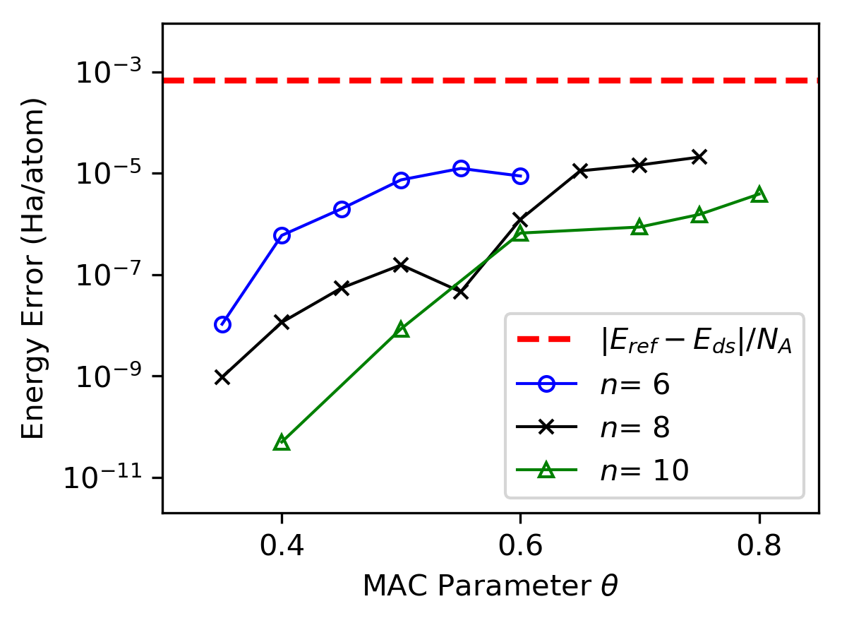
The sum in Eq. (32) is a discretization of the convolution integral in Eq. (31), and it is important to ensure that the treecode approximation error is less than discretization error. We document the accuracy of the treecode for the carbon monoxide molecule with domain a.u., quadrature order , mesh refinement tolerance 3e, SCF tolerance 1e, and Green Iteration tolerance 1e. In this case the number of mesh points is . We compute the ground-state energy with and without the treecode, and record the discretization error , and treecode approximation error , where is the reference energy computed by DFT-FE, and are computed by the present method using direct summation and the treecode, respectively. Throughout this work the source clusters and target batch size parameters are set to . Figure 10 shows that the discretization error of the present method is 6.56e Ha/atom (red dashed line), while the treecode approximation error is much smaller. This confirms that in this range of parameter values, the numerical errors introduced by the treecode do not upset the accuracy of the discretization.
6.5 Treecode Efficiency on a 6-core CPU and single GPU
This section documents the BLTC efficiency on a 6-core 2.6 GHz Intel Core i7 processor and a single NVIDIA Titan V GPU. The treecode was programmed in C, with OpenMP directives for parallelizing over multiple CPU cores and OpenACC directives for running on the GPU. As noted above, the GPU implementation takes advantage of the fact that the particle-cluster interaction in Eq. (34) and the approximation in Eq. (35) both have the same direct sum structure involving independent kernel evaluations. The GPU processes the particle-particle interactions between the target batch and source cluster in parallel without thread divergence; this is because the MAC applies uniformly to all particles in a given target batch [55]. In practice, interaction lists are precomputed for each target batch to identify the source clusters interacting with the batch.
The performance of the BLTC on both platforms is demonstrated by computing the Hartree energy in Eq. (8) for the carbon monoxide molecule using the electron density from the first SCF iteration. Results are shown in Table 4 using direct summation and the treecode, for quadrature order and mesh refinement parameter between 1e and 1e yielding the indicated mesh size . The direct sum energy values in the 3rd column converge as the mesh is refined, and the 4th column shows the corresponding discretization error using the value obtained with =1e-8 as the reference. The 5th column records the treecode approximation error for MAC and degree ; this is the difference between the value of computed by direct summation (column 3) and the value computed by the treecode (not shown). The results show that the treecode approximation error is well below the discretization error and within chemical accuracy.
The remainder of Table 4 records computation times on the 6-core CPU and GPU for direct summation (ds) and the treecode (tc). Averaging over the six runs in Table 4, direct summation runs 192 times faster on the GPU than on the 6-core CPU, while the treecode runs 70 times faster. On both platforms the treecode is faster than direct summation, and the speedup (ds/tc) increases as the mesh is refined; this is consistent with scaling for direct summation and scaling for the treecode. In particular, for the largest mesh size with approximately 2.2 million mesh points, the treecode computation time on the GPU is less than 18 s, which is about 4.5 times faster than direct summation.
| 6-core CPU time (s) | GPU time (s) | |||||||||
|---|---|---|---|---|---|---|---|---|---|---|
| (Ha) | ds error | tc error | ds | tc | ds/tc | ds | tc | ds/tc | ||
| 1e-3 | 141000 | 74.88640 | 6.20e-4 | 5.31e-7 | 70.42 | 26.24 | 2.68 | 0.39 | 0.47 | 0.82 |
| 1e-4 | 184750 | 74.87690 | 8.88e-3 | 1.20e-6 | 150.13 | 41.40 | 3.63 | 0.67 | 0.68 | 0.97 |
| 1e-5 | 249500 | 74.88668 | 9.00e-4 | 8.85e-6 | 216.17 | 80.32 | 2.69 | 1.13 | 1.13 | 1.00 |
| 1e-6 | 459500 | 74.88551 | 2.70e-4 | 3.68e-5 | 638.23 | 196.11 | 3.25 | 3.57 | 2.72 | 1.31 |
| 1e-7 | 928500 | 74.88574 | 4.00e-5 | 6.33e-6 | 2509.2 | 486.54 | 5.16 | 13.70 | 6.49 | 2.11 |
| 1e-8 | 2224375 | 74.88578 | na | 2.57e-6 | 15239.6 | 1373.90 | 11.09 | 78.31 | 17.27 | 4.54 |
6.6 BLTC Parallel Efficiency on a Single GPU node with 1, 2 or 4 GPUs
This subsection documents the parallel efficiency of the BLTC on a single GPU node running with 1, 2 or 4 GPUs, using OpenMP to parallelize across GPUs with one thread assigned to each GPU. The test system has 10 million particles randomly located in a cube interacting via the Coulomb kernel. The work is divided into two stages; stage 1 encompasses the precomputing tasks in lines 1-2 of Algorithm 3 and stage 2 encompasses the batch-cluster computing in line 3. Figure 11 shows the parallel efficiency of each stage and the entire computation as the number of GPUs increases from 1 to 4. The precompute stage scales less efficiently than the compute phase, due to some serial computation embedded in these tasks (85% on 2 GPUs, 63% on 4 GPUs), but this accounts for only a small fraction of the total computation time. The compute stage has close to ideal scaling (98% on 2 GPUs, 94% on 4 GPUs); moreover this stage accounts for a large fraction of the total computation time and therefore the treecode achieves 90% efficiency for the entire computation on 4 GPUs.


7 Ground State Energy Computations for Atoms and Molecules
The ground-state energy of several atoms (Li, Be, O) and small molecules (, CO, ) was computed using treecode-accelerated Green Iteration (TAGI) with the LDA exchange-correlation functional [58, 59]. For each system the SCF iteration continued until the density residual fell below 1e. was set to 3e for the first step in the SCF, then gradually reduced to 1e over the next four steps. The TAGI discretization parameters (quadrature order , adaptive mesh parameter ) and treecode parameters (degree , MAC ) were chosen to ensure chemical accuracy of 1 mHa/atom in the computed ground-state energy. The computations were performed on a single node, where the treecode (written in C with OpenMP+OpenACC) was run on the four GPUs and the remainder of the code (written in Python) was run in serial on one CPU core.
Table 5 presents the parameters and results for each system. The numerical parameters () are chosen to ensure chemical accuracy in the energy, and the heavier carbon and oxygen atoms require somewhat higher numerical resolution than the lighter hydrogen, lithium, and beryllium atoms. In particular, a larger mesh size requires slightly tighter treecode parameters (increasing degree from to , decreasing MAC from to ). Column 9 records the error in the ground-state energy computed by TAGI with respect to reference energies computed to mHa/atom accuracy with DFT-FE [26], showing that TAGI achieves chemical accuracy. Column 10 records the total wall clock computation time (s). The benzene molecule (C6H6, ) is the largest system considered; the computation used approximately 1.5 million mesh points and required less than 4 hours of wall clock time.
| system | error (Ha/atom) | time (s) | |||||||
|---|---|---|---|---|---|---|---|---|---|
| Li | 3 | 4 | 7e-6 | 232000 | 6 | 0.8 | -7.334051 | 4.59e-4 | 35.75 |
| Be | 4 | 3 | 1e-5 | 179712 | 6 | 0.8 | -14.445658 | 5.32e-4 | 29.35 |
| O | 8 | 4 | 3e-7 | 421000 | 6 | 0.8 | -74.469668 | -3.38e-4 | 143.09 |
| H2 | 2 | 3 | 1e-3 | 51200 | 6 | 0.8 | -1.13584 | 9.05e-4 | 6.67 |
| CO | 14 | 4 | 3e-7 | 661625 | 7 | 0.7 | -112.473372 | -7.21e-4 | 932.03 |
| C6H6 | 42 | 4 | 3e-6 | 1464500 | 8 | 0.6 | -230.193158 | -3.64e-4 | 13947.89 |
Figure 12 show 2D slices of the adaptively refined mesh and computed electron density for the carbon monoxide molecule 12a and benzene molecule 12b. Both molecules are located in the z=0 plane; for the CO molecule, the carbon atom is at (-1.06581,0,0) and the oxygen atom is at (+1.06581,0,0); for the benzene molecule, the six carbon atoms are at , , , and the six hydrogen atoms are at , , . The slices are taken in the plane and show the region a.u. in the -plane. The adaptive mesh successfully captures the variation in magnitude of the electron density.


8 Conclusions
We presented a real-space method for all-electron Kohn-Sham DFT computations called Treecode-Accelerated Green Iteration (TAGI). TAGI is based on a reformulation of the Kohn-Sham equations in which the eigenvalue problem for the energies and wavefunctions in differential form is recast as a fixed-point problem in integral form by convolution with the bound state Helmholtz Green’s function [41]. In each SCF iteration the fixed-points are computed by Green Iteration, where the convolution integrals are discretized on an adaptive mesh and the discrete convolution sums are efficiently evaluated using a GPU-accelerated treecode.
TAGI relies on several key techniques to achieve chemical accuracy and computational efficiency. First, the Fejér quadrature rule and adaptive mesh refinement based on integration of a test function are used to compute integrals and represent the fields. Second, singularity subtraction is applied to evaluate convolution integrals having singular kernels; in particular a standard scheme is used for the Yukawa kernel in the Green Iteration convolutions, and we developed a new scheme for the Coulomb kernel in the Hartree potential convolutions since the standard scheme is inapplicable in that case. Third, a gradient-free method is employed to update the eigenvalues in Green Iteration. Fourth, the fixed-point iteration for the wavefunctions and eigenvalues in Green Iteration is accelerated using Anderson mixing. Fifth, the discrete convolution sums are computed efficiently using a barycentric Lagrange treecode (BLTC), which reduces the operation count from to , where is the number of mesh points. The GPU implementation of the BLTC is facilitated by the properties of barycentric Lagrange interpolation including its scale-invariance and the fact that the particle-cluster approximation in Eq. (35) consists of independent kernel evaluations which can be evaluated concurrently [55].
We demonstrated the effect of these techniques on the carbon monoxide molecule. First, we investigated the quadrature rule and adaptive mesh refinement scheme, showing that the ground-state energy of the CO molecule is computed to within chemical accuracy of 1 mHa/atom using roughly 600,000 quadrature points and 4th order quadrature. Second, we demonstrated the effect of the singularity subtraction schemes; the ground-state computation was performed with and without singularity subtraction on a sequence of progressively refined meshes, and we observed a 100-fold reduction in error using singularity subtraction. Third, we compared three methods for updating the eigenvalues in Green Iteration, 1) Laplacian update using the Rayleigh quotient of the Hamiltonian differential operator, 2) gradient update using integration by parts to reduce the order of the operator, and 3) gradient-free update; on a wide range of meshes the gradient-free update yields a 10-fold improvement in accuracy over the gradient update, and a 100-fold improvement over the Laplacian update. Fourth, we investigated the convergence of Green Iteration in the first SCF iteration for the CO molecule, showing that the spectral gap in the Hamiltonian eigenvalues controls the rate of convergence of the eigenfunctions in Green Iteration; in particular, a small gap implies slow convergence of the eigenfunction ; the convergence rates were predicted and then verified computationally; finally we showed in the case of slow convergence, Green Iteration can be accelerated by applying Anderson mixing to the eigenpairs, yielding a 6-fold reduction in the number of iterations in this example. Fifth, we demonstrated the treecode’s ability to rapidly compute accurate approximations of the discrete convolution sums; in ground-state computations for the CO molecule, we showed that the treecode approximation error can be driven below the discretization error; we then demonstrated the speedup of the treecode over direct summation on both a 6-core CPU (parallelized with OpenMP) and a GPU (parallelized with OpenACC), achieving an 11 speedup on the CPU and a 4.5 speedup on the GPU; finally we observed a 70 speedup of the treecode running on the GPU in comparison with the CPU.
We then performed TAGI computations for several atoms and small molecules on a single node with 4 GPUs, and verified the accuracy of the ground-state energy with respect to reference values. The results demonstrate the chemical accuracy and computational efficiency afforded by TAGI on these benchmark systems.
In future work we will implement a distributed memory version of TAGI able to run on multiple nodes, relying on domain decomposition to treat larger systems. We will also consider a treecode based on barycentric Hermite interpolation, to more efficiently reach high accuracy regime needed in this application [72]. In addition, we will extend TAGI to pseudopotential computations using Optimized Norm-Conserving Vanderbilt (ONCV) pseudopotentials [73]; this will alleviate the need for significant mesh refinement near atomic nuclei and reduce the number of wavefunctions per atom, allowing TAGI to scale to larger systems.
Acknowledgement
This work was supported by National Science Foundation grant DMS-1819094, and the Michigan Institute for Computational Discovery and Engineering (MICDE) and Mcubed program at the University of Michigan. RK thanks Lunmei Huang and Li Wang for early discussions on the Green’s function approach to DFT. NV thanks Bikash Kanungo and Sambit Das for providing reference values and the single-atom radial data. Computational resources and services were provided by Advanced Research Computing-Technology Services (ARC-TS) at the University of Michigan.
References
- [1] P. Hohenberg, W. Kohn, Inhomogeneous Electron Gas, Phys. Rev. 136 (3B) (1964) B864–B871. doi:10.1103/PhysRev.136.B864.
- [2] W. Kohn, L. J. Sham, Self-Consistent Equations Including Exchange and Correlation Effects, Phys. Rev. 140 (4A) (1965) A1133–A1138. doi:10.1103/PhysRev.140.A1133.
- [3] K. Burke, Perspective on density functional theory, The Journal of Chemical Physics 136 (15) (2012) 150901. doi:10.1063/1.4704546.
- [4] R. O. Jones, Density functional theory: Its origins, rise to prominence, and future, Rev. Mod. Phys. 87 (2015) 897–923. doi:10.1103/RevModPhys.87.897.
- [5] N. Mardirossian, M. Head-Gordon, Thirty years of density functional theory in computational chemistry: an overview and extensive assessment of 200 density functionals, Molecular Physics 115 (19) (2017) 2315–2372. doi:10.1080/00268976.2017.1333644.
- [6] L. Lin, J. Lu, L. Ying, Numerical methods for Kohn-Sham density functional theory, Acta Numer. 28 (2019) 405–539. doi:10.1017/S0962492919000047.
- [7] G. Kresse, J. Furthmüller, Efficient iterative schemes for ab initio total-energy calculations using a plane-wave basis set, Phys. Rev. B 54 (16) (1996) 11169–11186. doi:10.1103/PhysRevB.54.11169.
- [8] X. Gonze, J.-M. Beuken, R. Caracas, F. Detraux, M. Fuchs, G.-M. Rignanese, L. Sindic, M. Verstraete, G. Zerah, F. Jollet, M. Torrent, A. Roy, M. Mikami, P. Ghosez, J.-Y. Raty, D. Allan, First-principles computation of material properties: the ABINIT software project, Comput. Mater. Sci. 25 (3) (2002) 478–492. doi:10.1016/S0927-0256(02)00325-7.
- [9] M. D. Segall, P. J. D. Lindan, M. J. Probert, C. J. Pickard, P. J. Hasnip, S. J. Clark, M. C. Payne, First-principles simulation: ideas, illustrations and the CASTEP code, J. Phys. Condens. Matter 14 (11) (2002) 2717–2744. doi:10.1088/0953-8984/14/11/301.
- [10] P. Giannozzi, S. Baroni, N. Bonini, M. Calandra, R. Car, C. Cavazzoni, D. Ceresoli, G. L. Chiarotti, M. Cococcioni, I. Dabo, A. Dal Corso, S. de Gironcoli, S. Fabris, G. Fratesi, R. Gebauer, U. Gerstmann, C. Gougoussis, A. Kokalj, M. Lazzeri, L. Martin-Samos, N. Marzari, F. Mauri, R. Mazzarello, S. Paolini, A. Pasquarello, L. Paulatto, C. Sbraccia, S. Scandolo, G. Sclauzero, A. P. Seitsonen, A. Smogunov, P. Umari, R. M. Wentzcovitch, Quantum ESPRESSO: a modular and open-source software project for quantum simulations of materials, J. Phys. Condens. Matter 21 (39) (2009) 395502. doi:10.1088/0953-8984/21/39/395502.
- [11] P. Giannozzi, O. Andreussi, T. Brumme, O. Bunau, M. Buongiorno Nardelli, M. Calandra, R. Car, C. Cavazzoni, D. Ceresoli, M. Cococcioni, N. Colonna, I. Carnimeo, A. Dal Corso, S. de Gironcoli, P. Delugas, R. A. DiStasio, A. Ferretti, A. Floris, G. Fratesi, G. Fugallo, R. Gebauer, U. Gerstmann, F. Giustino, T. Gorni, J. Jia, M. Kawamura, H.-Y. Ko, A. Kokalj, E. Küçükbenli, M. Lazzeri, M. Marsili, N. Marzari, F. Mauri, N. L. Nguyen, H.-V. Nguyen, A. Otero-de-la Roza, L. Paulatto, S. Poncé, D. Rocca, R. Sabatini, B. Santra, M. Schlipf, A. P. Seitsonen, A. Smogunov, I. Timrov, T. Thonhauser, P. Umari, N. Vast, X. Wu, S. Baroni, Advanced capabilities for materials modelling with Quantum ESPRESSO, J. Phys. Condens. Matter 29 (46) (2017) 465901. doi:10.1088/1361-648X/aa8f79.
- [12] T. Loucks, J. C. Slater, Augmented Plane Wave Method: A Guide to Performing Electronic Structure Calculations, in: Phys. Today, Vol. 20, 1967, pp. 92–93. doi:10.1063/1.3034041.
- [13] O. K. Andersen, Linear methods in band theory, Phys. Rev. B 12 (8) (1975) 3060–3083. doi:10.1103/PhysRevB.12.3060.
- [14] E. Wimmer, H. Krakauer, M. Weinert, A. J. Freeman, Full-potential self-consistent linearized-augmented-plane-wave method for calculating the electronic structure of molecules and surfaces: molecule, Phys. Rev. B 24 (2) (1981) 864–875. doi:10.1103/PhysRevB.24.864.
- [15] M. Weinert, E. Wimmer, A. J. Freeman, Total-energy all-electron density functional method for bulk solids and surfaces, Phys. Rev. B 26 (8) (1982) 4571–4578. doi:10.1103/PhysRevB.26.4571.
- [16] E. Sjöstedt, L. Nordström, D. Singh, An alternative way of linearizing the augmented plane-wave method, Solid State Commun. 114 (1) (2000) 15–20. doi:10.1016/S0038-1098(99)00577-3.
- [17] G. K. H. Madsen, P. Blaha, K. Schwarz, E. Sjöstedt, L. Nordström, Efficient linearization of the augmented plane-wave method, Phys. Rev. B 64 (19) (2001) 195134. doi:10.1103/PhysRevB.64.195134.
- [18] M. J. Frisch, G. W. Trucks, H. B. Schlegel, G. E. Scuseria, M. A. Robb, J. R. Cheeseman, G. Scalmani, V. Barone, G. A. Petersson, H. Nakatsuji, X. Li, M. Caricato, A. V. Marenich, J. Bloino, B. G. Janesko, R. Gomperts, B. Mennucci, H. P. Hratchian, J. V. Ortiz, A. F. Izmaylov, J. L. Sonnenberg, D. Williams-Young, F. Ding, F. Lipparini, F. Egidi, J. Goings, B. Peng, A. Petrone, T. Henderson, D. Ranasinghe, V. G. Zakrzewski, J. Gao, N. Rega, G. Zheng, W. Liang, M. Hada, M. Ehara, K. Toyota, R. Fukuda, J. Hasegawa, M. Ishida, T. Nakajima, Y. Honda, O. Kitao, H. Nakai, T. Vreven, K. Throssell, J. A. Montgomery, Jr., J. E. Peralta, F. Ogliaro, M. J. Bearpark, J. J. Heyd, E. N. Brothers, K. N. Kudin, V. N. Staroverov, T. A. Keith, R. Kobayashi, J. Normand, K. Raghavachari, A. P. Rendell, J. C. Burant, S. S. Iyengar, J. Tomasi, M. Cossi, J. M. Millam, M. Klene, C. Adamo, R. Cammi, J. W. Ochterski, R. L. Martin, K. Morokuma, O. Farkas, J. B. Foresman, D. J. Fox, Gaussian˜16 Revision B.01, gaussian Inc. Wallingford CT (2016).
- [19] M. Valiev, E. Bylaska, N. Govind, K. Kowalski, T. Straatsma, H. Van Dam, D. Wang, J. Nieplocha, E. Apra, T. Windus, W. de Jong, NWChem: A comprehensive and scalable open-source solution for large scale molecular simulations, Comput. Phys. Commun. 181 (9) (2010) 1477–1489. doi:10.1016/j.cpc.2010.04.018.
- [20] E. Tsuchida, M. Tsukada, Large-Scale Electronic-Structure Calculations Based on the Adaptive Finite-Element Method, J. Phys. Soc. Japan 67 (11) (1998) 3844–3858. doi:10.1143/JPSJ.67.3844.
- [21] J. E. Pask, B. M. Klein, C. Y. Fong, P. A. Sterne, Real-space local polynomial basis for solid-state electronic-structure calculations: A finite-element approach, Phys. Rev. B 59 (19) (1999) 12352–12358. doi:10.1103/PhysRevB.59.12352.
- [22] L. Lehtovaara, V. Havu, M. Puska, All-electron density functional theory and time-dependent density functional theory with high-order finite elements, J. Chem. Phys. 131 (5) (2009) 1–10. doi:10.1063/1.3176508.
- [23] P. Motamarri, M. Nowak, K. Leiter, J. Knap, V. Gavini, Higher-order adaptive finite-element methods for Kohn–Sham density functional theory, J. Comput. Phys. 253 (2013) 308–343. doi:10.1016/j.jcp.2013.06.042.
- [24] P. Motamarri, V. Gavini, Subquadratic-scaling subspace projection method for large-scale Kohn-Sham density functional theory calculations using spectral finite-element discretization, Phys. Rev. B 90 (11) (2014) 115127. doi:10.1103/PhysRevB.90.115127.
- [25] B. Kanungo, V. Gavini, Large-scale all-electron density functional theory calculations using an enriched finite-element basis, Phys. Rev. B 95 (3) (2017) 035112. doi:10.1103/PhysRevB.95.035112.
- [26] P. Motamarri, S. Das, S. Rudraraju, K. Ghosh, D. Davydov, V. Gavini, DFT-FE – A massively parallel adaptive finite-element code for large-scale density functional theory calculations, Comput. Phys. Commun. 246 (2020) 106853. doi:10.1016/j.cpc.2019.07.016.
- [27] S. Das, P. Motamarri, V. Gavini, B. Turcksin, Y. W. Li, B. Leback, Fast, scalable and accurate finite-element based ab initio calculations using mixed precision computing: 46 PFLOPS simulation of a metallic dislocation system, in: Int. Conf. High Perform. Comput. Networking, Storage Anal. SC, IEEE Computer Society, New York, NY, USA, 2019, pp. 1–11. doi:10.1145/3295500.3357157.
- [28] V. Rokhlin, Rapid solution of integral equations of scattering theory in two dimensions, J. Comput. Phys. 86 (2) (1990) 414–439. doi:10.1016/0021-9991(90)90107-C.
- [29] R. Jorgenson, R. Mittra, Efficient calculation of the free-space periodic Green’s function, IEEE Trans. Antennas Propag. 38 (5) (1990) 633–642. doi:10.1109/8.53491.
- [30] R. Coifman, V. Rokhlin, S. Wandzura, The fast multipole method for the wave equation: a pedestrian prescription, IEEE Antennas Propag. Mag. 35 (3) (1993) 7–12. doi:10.1109/74.250128.
- [31] L. N. Medgyesi-Mitschang, J. M. Putnam, M. B. Gedera, Generalized method of moments for three-dimensional penetrable scatterers, J. Opt. Soc. Am. A 11 (4) (1994) 1383. doi:10.1364/JOSAA.11.001383.
- [32] E. Bleszynski, M. Bleszynski, T. Jaroszewicz, AIM: Adaptive integral method for solving large-scale electromagnetic scattering and radiation problems, Radio Sci. 31 (5) (1996) 1225–1251. doi:10.1029/96RS02504.
- [33] J. L. Volakis, K. Sertel, Integral equation methods for electromagnetics, Scitech, 2011. doi:10.1049/SBEW045E.
- [34] M. M. Botha, Solving the volume integral equations of electromagnetic scattering, J. Comput. Phys. 218 (1) (2006) 141–158. doi:https://doi.org/10.1016/j.jcp.2006.02.004.
- [35] L. D. Faddeyev, B. Seckler, The Inverse Problem in the Quantum Theory of Scattering, J. Math. Phys. 4 (1) (1963) 72–104. doi:10.1063/1.1703891.
- [36] B. R. Johnson, D. Secrest, The Solution of the Nonrelativistic Quantum Scattering Problem without Exchange, J. Math. Phys. 7 (12) (1966) 2187–2195. doi:10.1063/1.1704905.
- [37] E. Alt, P. Grassberger, W. Sandhas, Reduction of the three-particle collision problem to multi-channel two-particle Lippmann-Schwinger equations, Nucl. Phys. B 2 (2) (1967) 167–180. doi:10.1016/0550-3213(67)90016-8.
- [38] R. I. Masel, R. P. Merrill, W. H. Miller, Quantum scattering from a sinusoidal hard wall: Atomic diffraction from solid surfaces, Phys. Rev. B 12 (12) (1975) 5545–5551. doi:10.1103/PhysRevB.12.5545.
- [39] S. K. Adhikari, Quantum scattering in two dimensions, Am. J. Phys. 54 (4) (1986) 362–367. doi:10.1119/1.14623.
- [40] K. T. Hecht, Operator Form of Scattering Green’s Function and the Integral Equation for the Scattering Problem, Springer New York, New York, NY, 2000, Ch. Scattering, pp. 477–480. doi:10.1007/978-1-4612-1272-0{\_}47.
- [41] M. H. Kalos, Monte Carlo Calculations of the Ground State of Three- and Four-Body Nuclei, Phys. Rev. 128 (4) (1962) 1791–1795. doi:10.1103/PhysRev.128.1791.
- [42] Z. Zhao, N. Kovvali, W. Lin, C.-H. Ahn, L. Couchman, L. Carin, Volumetric fast multipole method for modeling Schrödinger’s equation, J. Comput. Phys. 224 (2) (2007) 941–955. doi:10.1016/j.jcp.2006.11.003.
- [43] R. J. Harrison, G. I. Fann, T. Yanai, Z. Gan, G. Beylkin, Multiresolution quantum chemistry: Basic theory and initial applications, J. Chem. Phys. 121 (23) (2004) 11587–11598. doi:10.1063/1.1791051.
- [44] R. J. Harrison, G. Beylkin, F. A. Bischoff, J. A. Calvin, G. I. Fann, J. Fosso-Tande, D. Galindo, J. R. Hammond, R. Hartman-Baker, J. C. Hill, J. Jia, J. S. Kottmann, M. J. Ou, J. Pei, L. E. Ratcliff, M. G. Reuter, A. C. Richie-Halford, N. A. Romero, H. Sekino, W. A. Shelton, B. E. Sundahl, W. S. Thornton, E. F. Valeev, Á. Vázquez-Mayagoitia, N. Vence, T. Yanai, Y. Yokoi, Madness: A multiresolution, adaptive numerical environment for scientific simulation, in: SIAM J. Sci. Comput., Vol. 38, Society for Industrial and Applied Mathematics Publications, 2016, pp. S123–S142. arXiv:1507.01888, doi:10.1137/15M1026171.
- [45] M. J. Mohlenkamp, T. Young, Convergence of Green Iterations for Schrödinger Equations, Recent Adv. Comput. Sci. (2008) 201–208doi:10.1142/9789812792389{\_}0010.
- [46] M. J. Mohlenkamp, Function space requirements for the single-electron functions within the multiparticle Schrödinger equation, J. Math. Phys. 54 (6) (2013) 062105. doi:10.1063/1.4811396.
- [47] B. N. Khoromskij, On tensor approximation of Green iterations for Kohn-Sham equations, Comput. Vis. Sci. 11 (4-6) (2008) 259–271. doi:10.1007/s00791-008-0097-x.
- [48] M. V. Rakhuba, I. V. Oseledets, Fast Multidimensional Convolution in Low-Rank Tensor Formats via Cross Approximation, SIAM J. Sci. Comput. 37 (2) (2015) A565–A582. doi:10.1137/140958529.
- [49] M. V. Rakhuba, I. V. Oseledets, Grid-based electronic structure calculations: The tensor decomposition approach, J. Comput. Phys. 312 (2016) 19–30. doi:https://doi.org/10.1016/j.jcp.2016.02.023.
- [50] L. Fejér, Mechanische Quadraturen mit positiven Cotesschen Zahlen, Math. Zeitschrift 37 (1) (1933) 287–309. doi:10.1007/BF01474575.
- [51] L. N. Trefethen, Is Gauss quadrature better than Clenshaw-Curtis?, SIAM Rev. 50 (1) (2008) 67–87. doi:10.1137/060659831.
- [52] P. Rabinowitz, Approximate methods of higher analysis. L. V. Kantorovich and V. I. Krylov. translated from the third Russian edition by Curtis D. Benster. interscience, new york, 1959., Science 134 (3487) (1961) 1358–1358. doi:10.1126/science.134.3487.1358.
- [53] P. M. Anselone, Singularity subtraction in the numerical solution of integral equations, J. Aust. Math. Soc. Ser. B. Appl. Math. 22 (4) (1981) 408–418. doi:10.1017/S0334270000002757.
- [54] L. Wang, R. Krasny, S. Tlupova, A kernel-independent treecode based on barycentric Lagrange interpolation, arXiv e-printsarXiv:1902.02250.
- [55] N. Vaughn, L. Wilson, R. Krasny, A GPU-Accelerated Barycentric Lagrange Treecode, submitted (2020).
- [56] S. Goedecker, Linear scaling electronic structure methods, Rev. Mod. Phys. 71 (4) (1999) 1085–1123. doi:10.1103/RevModPhys.71.1085.
- [57] D. G. Anderson, Iterative Procedures for Nonlinear Integral Equations, J. ACM 12 (4) (1965) 547–560. doi:10.1145/321296.321305.
- [58] D. M. Ceperley, B. J. Alder, Ground State of the Electron Gas by a Stochastic Method, Phys. Rev. Lett. 45 (7) (1980) 566–569. doi:10.1103/PhysRevLett.45.566.
- [59] J. P. Perdew, A. Zunger, Self-interaction correction to density-functional approximations for many-electron systems, Phys. Rev. B 23 (10) (1981) 5048–5079. doi:10.1103/PhysRevB.23.5048.
- [60] M. A. L. Marques, M. J. T. Oliveira, T. Burnus, Libxc: A library of exchange and correlation functionals for density functional theory, Comput. Phys. Commun. 183 (10) (2012) 2272–2281. doi:https://doi.org/10.1016/j.cpc.2012.05.007.
- [61] S. Lehtola, C. Steigemann, M. J. Oliveira, M. A. Marques, Recent developments in libxc — A comprehensive library of functionals for density functional theory, SoftwareX 7 (2018) 1–5. doi:10.1016/j.softx.2017.11.002.
- [62] J. R. Chelikowsky, N. Troullier, Y. Saad, Finite-difference-pseudopotential method: Electronic structure calculations without a basis, Phys. Rev. Lett. 72 (8) (1994) 1240–1243. doi:10.1103/PhysRevLett.72.1240.
- [63] J. Bernholc, M. Hodak, W. Lu, Recent developments and applications of the real-space multigrid method, J. Phys. Condens. Matter 20 (29) (2008) 294205. doi:10.1088/0953-8984/20/29/294205.
- [64] Y. Saad, J. R. Chelikowsky, S. M. Shontz, Numerical Methods for Electronic Structure Calculations of Materials, SIAM Rev. 52 (1) (2010) 3–54. doi:10.1137/060651653.
- [65] L. N. Trefethen, Spectral methods in MATLAB, SIAM, 2008.
- [66] L. N. Trefethen, D. I. Bau, Numerical linear algebra, SIAM Society for Industrial and Applied Mathematics, 2000.
- [67] J. Barnes, P. Hut, A hierarchical O(N log N) force-calculation algorithm, Nature 324 (6096) (1986) 446–449. doi:10.1038/324446a0.
- [68] L. Greengard, V. Rokhlin, A fast algorithm for particle simulations, J. Comput. Phys. 73 (2) (1987) 325–348. doi:https://doi.org/10.1016/0021-9991(87)90140-9.
- [69] J.-P. Berrut, L. N. Trefethen, Barycentric Lagrange Interpolation, SIAM Rev. 46 (3) (2004) 501–517. doi:10.1137/S0036144502417715.
- [70] P. Li, H. Johnston, R. Krasny, A Cartesian treecode for screened coulomb interactions, J. Comput. Phys. 228 (10) (2009) 3858–3868. doi:10.1016/j.jcp.2009.02.022.
- [71] H. E. Salzer, Lagrangian interpolation at the Chebyshev points ; some unnoted advantages, Comput. J. 15 (1972) 156–159.
- [72] R. Krasny, L. Wang, A treecode based on barycentric Hermite interpolation for electrostatic particle interactions, Comput. Math. Biophys. 7 (2019) 73–84. doi:https://doi.org/10.1515/cmb-2019-0006.
- [73] D. R. Hamann, Optimized norm-conserving vanderbilt pseudopotentials, Phys. Rev. B - Condens. Matter Mater. Phys. 88 (8) (2013) 085117. doi:10.1103/PhysRevB.88.085117.
Appendix A Symbols
| Variables, fields, and operators | Symbol |
| Electron density, Eq. (4) | |
| Effective potential, Eq. (2) | |
| Hamiltonian operator, Eq. (1) | |
| Hamiltonian eigenpairs, Eq. (1) | |
| Green Function Integral operator, Eq. (12) | |
| Integral eigenpairs, Eq. (30) | |
| Physical parameters and constants | Symbol |
| Number of atoms, Eq. (3) | |
| Atomic positions, Eq. (3) | |
| Nuclear charges, Eq. (3) | |
| Number of electrons, Eq. (5) | |
| Boltzmann constant, Eq. (4) | |
| Temperature, Eq. (4) | |
| Fermi Energy, Eq. (5) | |
| Numerical Parameters | Symbol |
| Number of wavefunctions, Eq. (5) | |
| Mesh refinement parameter, Eq. (16) | |
| Number of cells, Eq. (14) | |
| Quadrature order, Eq. (14) | |
| Number of quadrature points, Eq. (14) | |
| SCF convergence tolerance, Alg. (1) | |
| Green Iteration convergence tolerance, Alg. (2) | |
| Anderson mixing parameter | |
| Gaussian singularity subtraction parameter, Eq. (23) | |
| Gauge shift, Eq. (22) | |
| Treecode MAC parameter, Eq. (36) | |
| Treecode interpolation degree, Eq. (35) | |
| Treecode maximum batch size | |
| Treecode maximum leaf cluster size | |
| Number if source particles in cluster |